


1 INTRODUCTION
‘Where is Population III?’ is an important question (Ishiyama et al. Reference Ishiyama, Sudo, Yokoi, Hasegawa, Tominaga and Susa2016) and often asked rhetorically. The question asked in this paper—whether population II stars are coeval and homogeneously distributed—is no less important for different reasons. Whether population II is present in all galaxies and is coeval everywhere places constraints on cosmology and galaxy formation and could impact theories such as timescape cosmology (Wiltshire Reference Wiltshire2009) or the multiverse (Rees Reference Rees2001; Linde Reference Linde2015). More generally, comparing the observed age of Population II stars to the age of the Universe constrains the cosmological constant and is one of the three pillars supporting the standard model of cosmology, the others being the anisotropy of the cosmic microwave background (Planck Collaboration et al. 2016a, CMB) and the Hubble diagram of type Ia supernovae (Turner, Reference Turner2001).
In this work, we examine the spatial distribution of tracers of population II stars: Globular Clusters (GCs) at low-redshift (Section 2) and at high-redshift, quasi-stellar objects (QSOs; Section 3) and the optical depth to reionisation along different lines of sight (Section 4). Motivated by the apparent isotropy in GCs and anisotropy in the high-z QSO distribution, we conclude by discussing the possibility of a non-coeval population II objects.
2 GLOBULAR CLUSTERS—LOCAL TRACERS OF OLD POP II OBJECTS
GCs have long been recognised as one of the oldest known stellar systems. Although many are probably destroyed over cosmic time, some survive till today, being ubiquitous around large galaxies and occasionally hosted by dwarf galaxies (see Brodie & Strader Reference Brodie and Strader2006 for a review). GC systems usually reveal a bimodal colour distribution, which is largely due to a ~1 dex difference in their metallicity (Usher et al. Reference Usher2012). These blue/metal-poor and red/metal-rich subpopulations of GCs may also have a small difference in their mean age with the red/metal-rich GCs being younger ~1 Gyr (although formally it is difficult to rule out coeval ages). Current absolute age estimates for Milky Way GCs, based on main sequence and white dwarf cooling fitting, indicates that the blue/metal-poor GCs were formed around 12.5 Gyr ago, however, the uncertainties on this value place the metal-poor GCs well within the epoch of reionisation (i.e., z > 6, age > 12.8 Gyr). Extragalactic GCs are less well constrained but are consistent with the old ages of their Galactic counterparts (Strader et al. Reference Strader, Brodie, Cenarro, Beasley and Forbes2005; Wagner-Kaiser et al. Reference Wagner-Kaiser2017). For a summary of GC ages from observational constraints, and predictions from various simulations, see Forbes et al. (Reference Forbes, Pastorello, Romanowsky, Usher, Brodie and Strader2015) and Mould (Reference Mould1998). More recently, a simulation of GC systems around Milky Way like galaxies by Pfeffer (Reference Pfeffer, Kruijssen, Crain and Bastian2018) predicts GCs to start forming before a redshift of 6 and continue to earlier times. Hubble Space Telescope (HST) observations, exploiting the amplification of strong lensing, have identified possible proto-GCs at z = 6.1 (Vanzella et al. Reference Vanzella2017). Another important feature of metal-poor GCs is that they appear to have a ‘metallicity floor’, i.e., no GC has been observed with a metallicity [Z/H] below −2.5 (e.g., Usher et al. (Reference Usher2012)). The reason for this minimum metallicity is not yet fully understood but may be a combination of pre-enrichment by Pop III stars (Beasley et al. Reference Beasley, Kawata, Pearce, Forbes and Gibson2003) and gas cooling by metals and molecules (Glover & Clark Reference Glover and Clark2014).
In Figure 1, we show the space distribution of known GC systems from the compilation of Harris et al. (Reference Harris, Harris and Alessi2013). Although this compilation does not separate the two subpopulations, previous work has shown the blue/metal-poor subpopulation is found in all GC systems unlike the red/metal-rich subpopulation that is increasingly absent in lower mass galaxies Peng et al. (Reference Peng2006). Thus, the distribution can be taken as a proxy for the old, population II metal-poor GCs. The GCs are isotropically distributed on the sky modulo the regions associated with the Galactic disk.
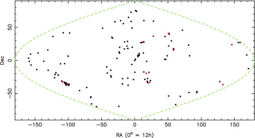
Figure 1. The shell of globular cluster systems beyond 20 Mpc. Globular clusters beyond 100 Mpc are shown in red, with the most distant being globular clusters located in Abell 1689 at 790 Mpc or 2.5 Glyr. Data are from the compilation of Harris et al. (Reference Harris, Harris and Alessi2013).
3 QUASARS—TRACING EARLY POP II OBJECTS
Given a conservative lower limit of 12 Gyrs for the age of Population II, these stars formed at z > 6 according to the standard model of cosmology with Planck collaboration parameters (Planck Collaboration et al. 2016a). Unfortunately, it is as yet infeasible to observe directly low-mass objects in this epoch, so we must rely on more luminous tracers of the star formation activity. We turn to quasars because (i) they are observationally feasible, and (ii) there is a well-discussed link between quasar activity and star formation rates in high-redshift galaxies. For instance, a positive correlation between quasar luminosity and far-IR luminosity has been seen previously (Wang et al. Reference Wang2011; Omont et al. Reference Omont, Willott, Beelen, Bergeron, Orellana and Delorme2013; Venemans et al. Reference Venemans2015). The spatial distribution of quasars at z > 6 in the Million Quasar CatalogFootnote 1 (Flesch Reference Flesch2015) is shown in Figure 2. Two features catch the eye: the Galactic plane, and some apparent voids. The dearth of high-z QSOs in the Galactic Plane is easily explained as obscuration by the Milky Way. The largest void is at 12 h right ascension and −60° declination. It appears to be of significant size (~1 Gpc in diameter), but this is an upper limit imposed by selection effects. The reasons for this apparent southern void are not understood, but likely fall into one of two camps. First, the void might be due to an unaccounted for selection effect related to the union of the heterogenous surveys that go into the Million Quasar Catalog. Second and more interestingly, the void could be real. If so, the void could point to large-scale anisotropies in the SFR at high-redshift in conflict with the predictions of the standard cosmological model.
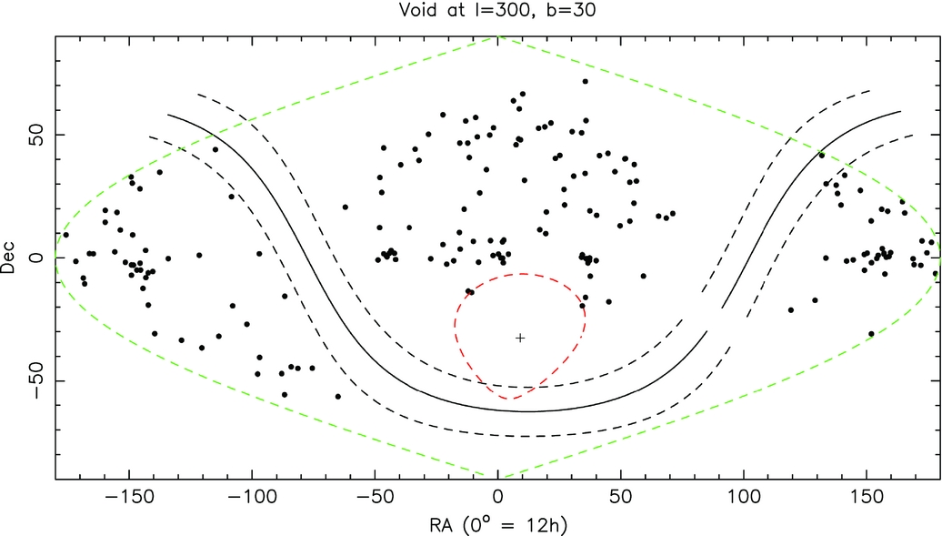
Figure 2. QSOs with z > 6 distributed on the sky. RA horizontal, Dec. vertical. We show the galactic plane ±10° and in green the boundaries of the projection. A 30° radius void is shown in red.
4 A HYPOTHETICAL VOID
For the sake of argument, let us suppose that the void in Figure 1 were real. This is a useful hypothesis to entertain as, if and when observers fill it, constraints on large-scale inhomogeneities (Section 1) will find application to cosmology. A Gpc-scale void in z > 6 QSOs begs the question: what triggers the formation of supermassive black holes (Wang et al. Reference Wang2017)? If reflected in the star-formation rate, as suggested by the established connection between QSO activity and SFR at lower redshifts, this void also poses a new question: could the reionisation of the Universe by the first stars be delayed on such enormous scales?
We can test this hypothesis even before the advent of 21 cm experiments by studying the CMB anisotropies in the direction of the hypothesised void. Measurements of the CMB power spectra have already led to constraints on the average optical depth to reionisation and thus the timing of reionisation. There are two main effects. First, the optical depth screens the primordial CMB anisotropies and suppresses the power by a factor e −2τ at all scales smaller than the horizon at the time of reionisation. Unfortunately, for measuring the mean optical depth, this signature is strongly degenerate with the amplitude of the primordial scalar perturbations power spectrum, A s. Second, Thomson scattering between the CMB quadrupole and the free electrons from reionisation generate linear polarisation at scales larger than the horizon size at the epoch of reionisation. This signal shows up in the CMB E and B −mode polarisation angular power spectra as a ‘bump’ at low multipoles, with the power scaling as τ2. The reionisation bump is not degenerate with other cosmological parameters, but careful cleaning of the galactic foregrounds is required at these angular scales, ℓ ≲ 10. The best constraints to date on the mean optical depth come from the Planck satellite, τ = 0.058 ± 0.012, suggesting that reionisation occurred around z re ~ 8 (Planck Collaboration et al. 2016b). Patchy reionisation has been explored by Roy et al. (Reference Roy, Lapi, Spergel and Baccigalupi2018).
4.1. Can we detect a lower optical depth towards the hypothetical void?
We can use current observations to go beyond the mean optical depth across the full sky. We expect reionisation to be a somewhat inhomogeneous process, and this inhomogeneity will cause variations in the optical depth integrated along different lines of sight. Broadly speaking, a larger value of τ in a given direction implies a higher z re and thus an earlier onset of star and galaxy formation; τ = 0 implies no reionisation at all. These variations in the optical depth will imprint a non-Gaussian signature in the CMB anisotropies. The non-Gaussianity can be detected with higher-order statistics of the map, as was done by Gluscevic, Kamionkowski, & Hanson (Reference Gluscevic, Kamionkowski and Hanson2013) and Namikawa (Reference Namikawa2017). In the future, these methods will be able to create maps of the optical depth across the sky (Dvorkin & Smith Reference Dvorkin and Smith2009).
In this work, we construct a simple estimator for the optical depth in the direction of the void and other similarly sized patches on the sky. Under the reasonable assumption that the primordial amplitude A s is constant, the power spectrum in a given direction will relate to the full-sky CMB spectrum according to  $\hat{C}^{TT}_{\ell }(\hat{\mathbf {n}}) = e^{-2(\tau (\hat{\mathbf {n}}) - \bar{\tau })}C_{\ell }^{TT,\,\rm full\,sky}$. Thus, variations in the power spectrum amplitude across the sky reflect variations in the optical depth τ. We use this idea to construct an estimator for the variation in the optical depth,
  $\delta \tau (\hat{\mathbf {n}}) = \tau (\hat{\mathbf {n}}) - \bar{\tau }$, as
 $$\begin{equation}
\delta \tau (\hat{\mathbf {n}}) = -\frac{1}{2}\ln \left( \frac{\sum _{\ell }\frac{\ell (\ell +1)}{2\pi }C^{TT}_{\ell }(\hat{\mathbf {n}})}{\sum _{\ell }\frac{\ell (\ell +1)}{2\pi }C^{TT, \,\rm full\,sky}_{\ell }}\right).
\end{equation}$$
$$\begin{equation}
\delta \tau (\hat{\mathbf {n}}) = -\frac{1}{2}\ln \left( \frac{\sum _{\ell }\frac{\ell (\ell +1)}{2\pi }C^{TT}_{\ell }(\hat{\mathbf {n}})}{\sum _{\ell }\frac{\ell (\ell +1)}{2\pi }C^{TT, \,\rm full\,sky}_{\ell }}\right).
\end{equation}$$
Details of how we calculate the power spectra and apply this estimator can be found in the appendix. If the lack of high-redshift quasars in one direction is due to a delay in the onset of star formation and reionisation, we would expect to see a lower optical depth and thus more CMB anisotropy power in that direction.
The hypothesis that the QSO void is associated with a late reionisation region, therefore, predicts a negative δτ in the direction of the void. To test this prediction, we estimate the optical depth over the z ~ 6 QSO void and also over a number of randomly positioned, same sized fields. The results are shown in Figure 3. In the plot, we also compare the distribution of the inferred τ values at the same locations for simulated noisy CMB temperature maps that do not include an inhomogeneous reionisation signal. The first thing we notice is that the τ distribution found for real data appears to be slightly more non-Gaussian than the one found for simulations. In particular, the distribution shows a positive τ tail, suggestive of early reionisation in some areas. We have tried varying the multipole range or reducing the mask radius to 5°, and find the positive tail in all cases although its magnitude changes. Interestingly, the relative optical depth found in the hypothetical QSO void is negative as would be expected for a region with delayed reionisation; however, the magnitude is not statistically significant. We have also varied the radius of the extracted region without significant change.
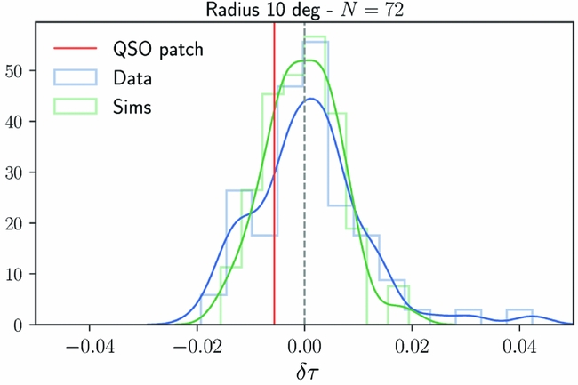
Figure 3. Histograms of the recovered optical depth fluctuations (with respect to the sky averaged value) in 72 randomly distributed circular patches of 10° radius. Blue colour shows the results for the Planck SMICA map while results based on the simulated map are shown in green. The vertical red line denotes the inferred value of τ in the hypothetical QSO void. The solid smooth lines represent kernel density estimates to the underlying distribution functions.
Looking to the future, observations of 21-cm emission from neutral hydrogen should prove useful for tracking a more detailed reionisation history and structure (Jacobs et al. Reference Jacobs2016; Roy et al. Reference Roy, Lapi, Spergel and Baccigalupi2018). Deep surveys continue to discover new galaxies at high redshifts (e.g., z > 10, Oesch et al. (Reference Oesch2016)), and the James Webb Space Telescope will provide even greater detection sensitivity for distant galaxies near the beginning of reionisation (Wang et al. Reference Wang2017). WFIRST may see and record the history of the formation of GC systems (Renzini Reference Renzini2017). Improved constraints on τ are also expected from future high sensitivity observations of CMB polarisation signals, such as CMB-S4 (Abazajian et al. Reference Abazajian2016) or the proposed CMBPol satellite (Zaldarriaga et al. Reference Zaldarriaga2008). Su et al. (Reference Su, Yadav, McQuinn and Yoo2011) have considered inhomogeneous reionisation and conclude that experiments such as CMBPol will be able to achieve a detection.
5 CONCLUSION
The apparent homogeneity in the extragalactic GC distribution sets a lower bound on the radius of possible voids in population II of ~80 Mpc in diameter (Appendix B). This is larger than the expectations of patchy reionisation (Roy et al. Reference Roy, Lapi, Spergel and Baccigalupi2018; Mutch et al. Reference Mutch, Geil, Poole, Angel, Duffy, Mesinger and Wyithe2016). The apparent void in the high z QSO distribution provides an upper limit of order a Gpc.
There are a number of avenues by which inhomogeneities in Population II can be detected and confirmed. These include deeper all sky mapping of QSOs with z > 6 (e.g., Taipan, da Cunha et al. Reference Cunha2017), deep HST imaging of rich GC systems at z > 0.1, polarisation mapping of the CMB and imaging of reionisation at 21 cm. This in turn will constrain some non-standard inhomogeneous cosmologies, such as timescape and the multiverse.
ACKNOWLEDGEMENTS
Parts of this research were conducted by the Australian Research Council Centre of Excellence for All-Sky Astrophysics under grant CE110001020. FB acknowledges support from an Australian Research Council Future Fellowship (FT150100074). Some of the results in this paper have been derived using the HEALPix (Gorski et al. Reference Gorski, Hivon, Banday, Wandelt, Hansen, Reinecke and Bartelmann2005) package. We thank an anonymous referee for helpful comments.
APPENDIX A: OPTICAL DEPTH ESTIMATOR AND POWER SPECTRUM ESTIMATION
In this appendix, we describe the power spectrum estimation and motivation for the specific form of the estimator in more detail.
A.1. Masks
The first step in calculating a CMB power spectrum is to define the mask on the sky over which the spectrum will be taken. We begin by creating a baseline, ‘full-sky’ mask. This is the 20% galactic mask (f sky = 0.8) provided by the Planck collaboration. We apodise the edges with a 2° taper and also mask point sources detected in the high-frequency Planck channels. This mask is used to calculate the full-sky CMB spectrum following the procedure below.
We also want to create masks that select specific regions of the sky. Based on the alleged QSO void morphology, we construct circular masks of 10° radius that we apodise with a Gaussian taper of FWHM of 30 arcmin. These circular masks are multiplied by the full-sky mask in order to avoid the galaxy or bright sources. We also impose a restriction that the circles overlap by less than 30%. With this restriction, the size of the circular mask dictates the number of roughly independent patches on the sky. We find 72 random locations for 10° radius circular patches.
A.2. Power spectrum estimation
For each mask, we measure cross-spectra between the two half-mission foreground-cleaned SMICA CMB temperature mapsFootnote 2 (provided in the HEALPixFootnote 3 format at an angular resolution of 5 arcmin) to avoid noise debiasing. We smoothly bandpass the temperature maps between 200 < ℓ < 2000 on the full-sky before extracting the cross-spectra on individual patches. The effect of masking, beam smoothing, and pixelation on the recovered spectra is taken into account through the use of the MASTER algorithm (Hivon et al. 2002). The reference full-sky power spectrum (the denominator in equation (1)) is estimated with the baseline mask above. The numerator is calculated from one of the circular masks.
A.3. Further details on the estimator
There are three points to note about equation (1). First, the sum is over a multipole range ℓ ∈ [300, 1900]. The lower end of this range is set by the finite size of the circular patches, while the upper end is selected based on where instrumental noise and foregrounds become significant. Second, we have chosen to use  $\frac{\ell (\ell +1)}{2\pi } C_\ell$ instead of C ℓ in the sum to avoid over-weighting large angular scales. Finally, the estimator uses the ratio of the summed power instead of summing ratios for stability reasons.
We note that the existence of a positive tail in the real distribution is robust to these analysis choices, although the magnitude of the tail varies. The same phenomenology is seen if the radius of the circular regions is reduced to 5°; the limited number of patches makes it hard to draw conclusions when the radius is instead increased to 20°. Positive tails are likewise still seen then the multipole range is varied by either increasing the lower limit to 650 or decreasing the upper limit to 1 100 or 1 600. A positive tail corresponds to lines of sight that undergo earlier reionisation.
APPENDIX B
We replot Figure 1 in three dimensions in Figure B1, using the distances of Harris et al. (Reference Harris, Harris and Alessi2013) and zooming in on the central 100 Mpc cube.
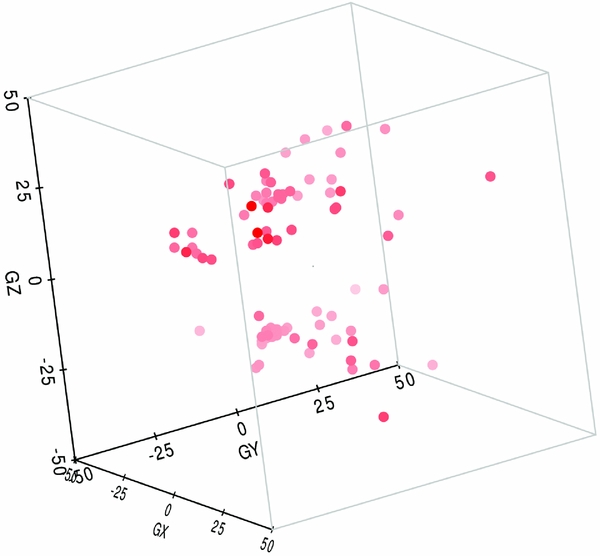
Figure B1. The globular cluster distribution in Galactic cartesian coordinates. GZ = 0 is the Galactic plane. The units are Mpc and the observer is at the origin. Red shading corresponds to depth in the plot. The distribution resembles a filled sphere with radius 40 Mpc after removal of an obscured area in the Galactic plane. This places a lower limit on the size of a local hypothetical population II void.


