


1. Introduction
The highly redshifted 21-cm signal of neutral hydrogen gas encodes the perturbation statistics of hyperfine states of neutral hydrogen gas, which trace the conditions of the radiation fields permeating the early universe. Measurements of this signal are therefore a promising path for further constraints on the Epoch of Reionization (EoR) and dark energy. Several experiments aiming to detect the 21-cm EoR signal are either complete or under way, such as the Donald C. Backer Precision Array for Probing the Epoch of Reionization (PAPER; Parsons et al. Reference Parsons2010), the Low-Frequency Array (LOFAR; van Haarlem et al. Reference van Haarlem, Wise, Gunst, Heald, McKean, Hessels and de Bruyn2013), the Murchison Widefield Array (MWA; Tingay et al. Reference Tingay2013a; Bowman et al. Reference Bowman2013), the Giant Metrewave Radio Telescope (GMRT; Gupta et al. Reference Gupta2017), and the Hydrogen Epoch of Reionization Array (HERA; DeBoer et al. Reference DeBoer2017).
However, the astrophysical foregrounds are four to five orders of magnitude brighter than the faint cosmological signal. But because the foregrounds are spectrally smooth, while the 21-cm signal has significant spectral structure, they can be in principle distinguished after performing a Fourier transform in frequency. The key challenges are precise calibration of the complicated frequency dependence of the instruments, accurate avoidance of radio frequency interference (RFI), and the effects of the ionospheric activity. Significant work in the past decade has led to a number of techniques aimed at overcoming these difficulties: data quality metrics to flag channels contaminated by RFI (Wilensky et al. Reference Wilensky, Morales, Hazelton, Barry, Byrne and Roy2019; Li et al. Reference Li, Pober, Berry and Hazelton2019; Kerrigan et al. Reference Kerrigan2019; Offringa et al. Reference Offringa2015), metrics to assess ionospheric activity (Jordan et al. Reference Jordan2017; Trott et al. Reference Trott2018), and a variety of instrumental calibration methods (e.g. Liu et al. Reference Liu, Tegmark, Morrison, Lutomirski and Zaldarriaga2010; Barry et al. Reference Barry, Beardsley, Byrne, Hazelton, Morales, Pober and Sullivan2019a; Yatawatta Reference Yatawatta2015).
A leading paradigm of 21-cm analysis is to measure the power spectrum (PS) of the signal in two-dimensional (2D) cylindrical Fourier space (i.e. the
 $(k_{\perp},k_{\parallel})$
plane, with Fourier modes perpendicular and parallel to the plane of the sky, respectivelyFootnote a. In the 2D
$(k_{\perp},k_{\parallel})$
plane, with Fourier modes perpendicular and parallel to the plane of the sky, respectivelyFootnote a. In the 2D
 $(k_{\perp},k_{\parallel})$
plane, foregrounds are confined to a wedge-shaped region, called the ‘foreground wedge’. The remaining region, namely the ‘EoR window’, is expected to be contaminant-free (Pober et al. Reference Pober2014; Datta, Bowman, & Carilli Reference Datta, Bowman and Carilli2010; Parsons et al. Reference Parsons, Pober, Aguirre, Carilli, Jacobs and Moore2012; Morales et al. Reference Morales, Hazelton, Sullivan and Beardsley2012; Vedantham, Shankar, & Subrahmanyan Reference Vedantham, Shankar and Subrahmanyan2012; Thyagarajan et al. Reference Thyagarajan2013; Trott, Wayth, & Tingay Reference Trott, Wayth and Tingay2012; Liu, Parsons, & Trott Reference Trott2014).
$(k_{\perp},k_{\parallel})$
plane, foregrounds are confined to a wedge-shaped region, called the ‘foreground wedge’. The remaining region, namely the ‘EoR window’, is expected to be contaminant-free (Pober et al. Reference Pober2014; Datta, Bowman, & Carilli Reference Datta, Bowman and Carilli2010; Parsons et al. Reference Parsons, Pober, Aguirre, Carilli, Jacobs and Moore2012; Morales et al. Reference Morales, Hazelton, Sullivan and Beardsley2012; Vedantham, Shankar, & Subrahmanyan Reference Vedantham, Shankar and Subrahmanyan2012; Thyagarajan et al. Reference Thyagarajan2013; Trott, Wayth, & Tingay Reference Trott, Wayth and Tingay2012; Liu, Parsons, & Trott Reference Trott2014).
For perfectly calibrated instruments, signal in the EoR window should only come from 21-cm signal emission in an uncontaminated observation. But in practice, small chromatic instrumental calibration errors introduce spectral structure in astrophysical foregrounds, which contaminates some Fourier modes in the EoR window and thus overwhelms the cosmological PS (Morales et al. Reference Morales, Beardsley, Pober, Barry, Hazelton, Jacobs and Sullivan2019; Barry et al. Reference Barry, Hazelton, Sullivan, Morales and Pober2016).
The two most popular methods of interferometric gain calibration are ‘sky-based’ and ‘redundant’, both are subject to systematic errors. Sky-based calibration uses deep foreground catalogues or maps to create model visibilities for calibration, which requires an accurate sky model; errors are introduced if the model does not capture the true sky brightness distribution. In particular, Barry et al. (Reference Barry, Hazelton, Sullivan, Morales and Pober2016) identified a specific class of calibration errors where the instrument’s point spread function interacts with missing sources in the sky model to introduce chromatic errors and couple foreground power into the EoR window. Redundant calibration takes advantage of the fact that any given correlation should depend only on relative positions of two antennas, which reduces a large number of unknowns when calibrating an redundant array. Redundant calibration is, to first order, sky-model-independent but may be contaminated by non-redundancy introduced through beam variation and antenna position errors (Orosz et al. Reference Orosz, Dillon, Ewall-Wice, Parsons and Thyagarajan2019; Joseph et al. Reference Joseph, Trott, Wayth and Nasirudin2019). Joseph, Trott, & Wayth (Reference Joseph, Trott and Wayth2018) found that the position offsets introduce a phase bias of the calibration solutions. This phase bias increases with the distance between bright radio sources and the pointing centre, and with the flux density of these sources (Joseph et al. Reference Joseph, Trott and Wayth2018). Byrne et al. (Reference Byrne2019) also showed that calibration errors caused by sky model incompleteness affect redundant calibration, since redundant calibration leaves degenerate parameters that must be constrained via reference to a sky model.
Although the principles and limitations of each calibration method are reasonably well understood, the actual performance of these techniques will be affected by realistic constraints, such as algorithm implementations, array configuration, sky model accuracy, and data contamination from interference. Recent analysis with the HERA telescope shows the potential for redundant calibration to provide some degree of information beyond sky calibration, as well as its value as a data quality metric (Kern et al. Reference Kern2020; Dillon et al. Reference Dillon2020). Li et al. (Reference Li2018) used the compact array of Phase II of the MWA (Wayth et al. Reference Wayth2018; Beardsley et al. Reference Beardsley2019), which has both large numbers of redundant baselines and a relatively complete sampling of Fourier space (i.e. UV coverage), to compare redundant calibration with sky-based algorithms in the EoR0 field (see Section 2 for a description of the fields observed by the MWA EoR project). That work showed that the tandem combination of sky-based calibration and redundant calibration yielded small but non-negligible reductions in foreground contamination in certain modes of the EoR PS. However, Li et al. (Reference Li, Pober, Berry and Hazelton2019) performed a similar analysis after adding an improved auto-correlation-based technique to the sky-based calibration step and found that the improvements brought about by redundant calibration became negligible. In this paper, we further investigate the performance of tandem redundant plus sky-based calibration in MWA Phase II data analysis in the EoR1 field, where we find a different result than that of Li et al. (Reference Li, Pober, Berry and Hazelton2019): redundant calibration has a significant positive impact on foreground contamination in the PS even with the auto-correlation-based technique applied to sky-based calibration (as will be shown in Section 4.3). Before presenting the PS results, we compare the calibration solutions derived from both sky and redundant calibration on a 2-min cadence from three nights of EoR1 and one night of EoR0 to investigate differences in the solutions themselves. As in Li et al. (Reference Li, Pober, Berry and Hazelton2019), we use packages Fast Holographic Deconvolution (FHD) and OMNICAL for state-of-the-art implementations of sky-based and redundant calibration, respectively.
The organisation of this paper is as follows. In Section 2, we describe the compact array of MWA Phase II and the observations analysed in this work. In Section 3, we review the methodology and mathematical framework of sky-based calibration and redundant calibration. In Section 4, we present all our analyses and results, including simulations exploring redundant calibration performance (Section 4.1), inspection of the calibration solutions themselves (Section 4.2), and PS analyses (Section 4.3). We further discuss over these analyses and present our conclusions in Section 5.
2. Observations
The MWA is a low-frequency (80–300 MHz) radio interferometer located at the Murchison Radio-astronomy Observatory in Western Australia, the location of the future low-frequency Square Kilometre Array. In MWA Phase I (2013–2016; Tingay et al. Reference Tingay2013b; Bowman et al. Reference Bowman2013), 128 antenna tilesFootnote b were arranged in a pseudo-random layout designed for excellent instantaneous UV coverage. The Phase II upgrade (Wayth et al. Reference Wayth2018; Beardsley et al. Reference Beardsley2019) added 128 additional tiles in mid-2016. The correlator is still limited to processing only 128 tiles at a time, so the array is periodically reconfigured between ‘compact’ and ‘extended’ configurations. The MWA Phase II compact array (Figure 1) consists of 72 tiles in a regular hexagonal grid and 56 pseudo-random tiles in a dense core with minimal redundancy. This configuration allows us to perform redundant calibration while retaining good UV coverage.
The individual dipoles in each tile can be time-delayed relative to each other in the beamformer, enabling the array to be ‘pointed’ to a certain patch of the sky. However, the time delays can only be adjusted by discrete amounts (as they are added by inserting additional physical lengths of cable into the signal chain), meaning that the telescope cannot continuously track a patch of sky. Instead, the MWA EoR program observes in a specific direction with the sky drifting overhead for about 30 min and then repoints the tiles to track the field of interest, which is called the ‘drift and shift’ method (Trott Reference Trott2014). During an observation, the delays are shifted multiple times until the field is too low in the sky to track, so the data in the observation are grouped into ‘pointings’ (each set of tile delays corresponds to one pointing). With the sky transiting from the east, the program begins observing at 5 pointings before zenith and ends observing at 4 pointings after zenith. The zenith is labelled as ‘pointing 0’, thus all the 10 pointings are labelled from pointing
 $-5$
to pointing 4.
$-5$
to pointing 4.
The MWA EoR program focuses on three fields with relatively low foreground emission: ‘EoR0’ (
 $\textrm{RA}=0^{\textrm{h}}00$
,
$\textrm{RA}=0^{\textrm{h}}00$
,
 $\textrm{Dec}=-27^{\circ}$
), ‘EoR1’ (
$\textrm{Dec}=-27^{\circ}$
), ‘EoR1’ (
 $\textrm{RA}=4^{\textrm{h}}00$
,
$\textrm{RA}=4^{\textrm{h}}00$
,
 $\textrm{Dec} = -27^{\circ}$
), and ‘EoR2’ (
$\textrm{Dec} = -27^{\circ}$
), and ‘EoR2’ (
 $\textrm{RA}=11^{\textrm{h}}33$
,
$\textrm{RA}=11^{\textrm{h}}33$
,
 $\textrm{Dec} = -10^{\circ}$
); see Jacobs et al. (Reference Jacobs2016) for the motivation for selecting these fields and Trott et al. (Reference Trott2020) for a detailed analysis of the features present in each. Each field fills the main lobe of the MWA primary beam, spanning roughly
$\textrm{Dec} = -10^{\circ}$
); see Jacobs et al. (Reference Jacobs2016) for the motivation for selecting these fields and Trott et al. (Reference Trott2020) for a detailed analysis of the features present in each. Each field fills the main lobe of the MWA primary beam, spanning roughly
 ${\sim}40^{\circ}$
on a side.
${\sim}40^{\circ}$
on a side.
In this work, we analyze high band (167–197 MHz) data from three nights observing EoR1 and one night observing EoR0. The most salient difference between these two fields is the presence of Fornax A, a bright, extended source in the EoR1 field; EoR0, in comparison, contains mostly unresolved sources. In this work, we denote the nights as ‘EoR1 night1’ (2016 October 15), ‘EoR1 night2’ (2016 October 17), ‘EoR1 night3’ (2016 November 15), and the ‘EoR0 night’ (2016 November 21), respectively. We explore the four nights using good pointings determined by the window power metric (Beardsley et al. Reference Beardsley2016; Li et al. Reference Li, Pober, Berry and Hazelton2019) and the ionospheric metric (Jordan et al. Reference Jordan2017; Trott et al. Reference Trott2018): for EoR1 night1 and night2, good pointings are −3, −2, −1, and 0; for EoR1 night3, good pointings are −3, −2, and −1; for the EoR0 night, good pointings are −2, −1, 0, 1, and 2.
The MWA uses the AOFlagger algorithmFootnote c to flag data contaminated by RFI (Offringa et al. Reference Offringa2015). In this work, we further flag faint RFI not captured by the pipeline using data quality metrics developed by Wilensky et al. (Reference Wilensky, Morales, Hazelton, Barry, Byrne and Roy2019) and Li et al. (Reference Li, Pober, Berry and Hazelton2019).
3. Calibration formalism
The sky signal is modified along the path from where it was emitted to where it was recorded. In order to measure the cosmological signal, all these modifications must be corrected for. While our RFI flagging and data quality metrics are used to avoid the most corrupted sky signals, the electronic response of the antennas must still be corrected for with a gain calibration algorithm.
In this section, we will briefly introduce two calibration methods used in our analysis: sky-based calibration and redundant calibration, and the code packages and algorithms we use to implement them.
3.1. Measurements of the sky
Suppose antenna i with gain
 $g_i$
measures a frequency domain signal
$g_i$
measures a frequency domain signal
 $s_i$
at a given instant, an approximation of a short time block.
$s_i$
at a given instant, an approximation of a short time block.
 $s_i$
is related to the true sky signal
$s_i$
is related to the true sky signal
 $h_i$
and the antenna’s instrumental noise contribution
$h_i$
and the antenna’s instrumental noise contribution
 $n_i$
as:
$n_i$
as:
 \begin{equation} s_i=g_i h_i+n_i,\end{equation}
which is both an equation of time and frequency.
In this paper, we consider only a single linear polarisation at a time. We assume per-antenna and per-frequency gains. In the MWA, the instrumental gains are assumed to be constant over 2-min observations. Then in a long integration time that
 $\langle n_i \rangle=0$
, the baseline
$\langle n_i \rangle=0$
, the baseline
 $b_{ij}$
measures the correlation between signals from antenna i and j (
$b_{ij}$
measures the correlation between signals from antenna i and j (
 $i\not= j$
):
$i\not= j$
):
 \begin{align} &v_{ij}=\langle s_i^*s_j\rangle \end{align}
 \begin{align} &\approx g_i^* g_j \langle h_i^*h_j\rangle+\langle n_i^*n_j\rangle+g_j\langle n_i^*h_j\rangle+g_i^*\langle h_i^*n_j\rangle \end{align}
 \begin{align}&= g_i^* g_j u_{ij}+n_{ij}, \end{align}
where
 $u_{ij}=\langle h_i^*h_j\rangle$
denotes the true visibility and
$u_{ij}=\langle h_i^*h_j\rangle$
denotes the true visibility and
 $n_{ij}$
is the residual noise as the synthesis of all noise contributions in Equation (2b). We have applied two assumptions: the noise of different antennas are uncorrelated and the sky signal does not correlate with the noise. Under these assumptions, the last three terms in Equation (2b) all have an expectation value of 0 in the limit that time goes to infinity. However, since our integration length is finite, these three terms contribute an approximately
$n_{ij}$
is the residual noise as the synthesis of all noise contributions in Equation (2b). We have applied two assumptions: the noise of different antennas are uncorrelated and the sky signal does not correlate with the noise. Under these assumptions, the last three terms in Equation (2b) all have an expectation value of 0 in the limit that time goes to infinity. However, since our integration length is finite, these three terms contribute an approximately
 $u_i$
-independent Gaussian random component, which we relabel as a single effective noise term
$u_i$
-independent Gaussian random component, which we relabel as a single effective noise term
 $n_{ij}$
in going to Equation (2c).
$n_{ij}$
in going to Equation (2c).
Our goal is to solve for the true sky visibilities
 $u_{ij}$
. Numerous algorithms and strategies have been developed for precise calibration. Most of them can be classified into two approaches: sky-based calibration and redundant calibration. We will briefly introduce both of the two calibration methods in Section 3.2.
$u_{ij}$
. Numerous algorithms and strategies have been developed for precise calibration. Most of them can be classified into two approaches: sky-based calibration and redundant calibration. We will briefly introduce both of the two calibration methods in Section 3.2.
3.2. Calibration techniques
In our analysis, we used two calibration packages: one is the FHDFootnote d (Barry et al. Reference Barry, Beardsley, Byrne, Hazelton, Morales, Pober and Sullivan2019a; Sullivan et al. Reference Sullivan2012) software pipeline, which is used for sky-based calibration, and the other is OMNICALFootnote e (Zheng et al. Reference Zheng2014), performing redundant calibration.Footnote f
They are two different methods but both work on maximum-likelihood estimate of per-frequency antenna gains. For any baseline
 $b_{ij}$
, we assume its noise is Gaussian and mean zero with variance
$b_{ij}$
, we assume its noise is Gaussian and mean zero with variance
 $\sigma_{ij}^2$
(Thompson, Moran, & Swenson Reference Thompson, Moran and Swenson George2017). Maximising the likelihood function of gains is equivalent to minimising
$\sigma_{ij}^2$
(Thompson, Moran, & Swenson Reference Thompson, Moran and Swenson George2017). Maximising the likelihood function of gains is equivalent to minimising
 \begin{equation} \chi^2=\sum_{ij}\frac{|v_{ij}-g_i^*g_j u_{ij}|^2}{\sigma^2_{ij}}.\end{equation}
Instrumental frequency dependence is implicit in this equation.
3.2.1. FHD: Sky-based calibration
Sky-based calibration works by substituting model visibilities for the true visibilities in Equation (3). The accuracy of the model visibilities determines the accuracy of sky-based calibration. We use GaLactic and Extragalactic All-sky MWA (GLEAM) (Hurley-Walker et al. Reference Hurley-Walker2016), an extragalactic point source catalogue with large coverage and high completeness, as our model sky to generate model visibilities. FHD simulates all reliable sources in the catalogue out to typically 1% beam level in the primary lobe and the sidelobes to build a theoretical sky (Barry et al. Reference Barry, Beardsley, Byrne, Hazelton, Morales, Pober and Sullivan2019a; Beardsley et al. Reference Beardsley2016). In this work, we exclude baselines shorter than 50 wavelengths (which are sensitive to diffuse Galactic emission absent from GLEAM) to reduce the contamination from differences between the model visibilities and the true visibilities (Barry et al. Reference Barry, Beardsley, Byrne, Hazelton, Morales, Pober and Sullivan2019a).
FHD calibration begins with a set of estimated initial solutions for
 ${g_i^*(\,f)}$
and the sky visibilities are substituted with model visibilities
${g_i^*(\,f)}$
and the sky visibilities are substituted with model visibilities
 $m_{ij}$
. (In practice, the digital gains in the MWA correlator pre-scale the visibilities to roughly the right level—so an initial gain estimate of 1.0 at for all antennas at all frequencies is sufficient for quick convergence of the calibration algorithm.) Then minimising Equation (3) becomes a linear least-squares problem:
$m_{ij}$
. (In practice, the digital gains in the MWA correlator pre-scale the visibilities to roughly the right level—so an initial gain estimate of 1.0 at for all antennas at all frequencies is sufficient for quick convergence of the calibration algorithm.) Then minimising Equation (3) becomes a linear least-squares problem:
 \begin{equation} \chi_{j,sky}^2(\,f)=\sum_{i}\frac{|v_{ij}(\,f)-g_i^*(\,f)g_j(\,f) m_{ij}(\,f)|^2}{\sigma^2_{ij}(\,f)},\end{equation}
where
 $m_{ij}$
is the model visibility. This relation can be solved iteratively to return the values of the g terms that minimise
$m_{ij}$
is the model visibility. This relation can be solved iteratively to return the values of the g terms that minimise
 $\chi^2$
(Mitchell et al. Reference Mitchell2008; Salvini & Wijnholds Reference Salvini and Wijnholds2014).
$\chi^2$
(Mitchell et al. Reference Mitchell2008; Salvini & Wijnholds Reference Salvini and Wijnholds2014).
Sky-based calibration requires an accurate sky model, otherwise the difference between the true sky visibilities and model visibilities will be incorporated into our evaluations of instrumental gains. Barry et al. (Reference Barry, Hazelton, Sullivan, Morales and Pober2016) demonstrate how gain errors due to sky model incompleteness introduce contamination that prevents recovery of an EoR signal.
3.2.2. OMNICAL: Redundant calibration
If an array is built to have sufficient redundant baselines, the total number of measurements will exceed the sampled points in Fourier space. In this case, our equations are over-determined and we are able to directly solve for both instrumental gains and visibilities (Liu et al. Reference Liu, Tegmark, Morrison, Lutomirski and Zaldarriaga2010). Pedagogically, we can understand this calibration method as minimising
 \begin{equation} \chi_\textrm{red}^2(\,f)=\sum_{\alpha}\sum_{\{i,j\}_{\alpha}}\frac{|v_{ij}(\,f)-g_i^*(\,f)g_j(\,f) u_{\alpha}(\,f)|^2}{\sigma^2_{ij}(\,f)},\end{equation}
where
 $\alpha$
indexes types of redundant baselines and
$\alpha$
indexes types of redundant baselines and
 $\{i,j\}_{\alpha}$
are sets of antennas that belong to each type of redundant baseline.
$\{i,j\}_{\alpha}$
are sets of antennas that belong to each type of redundant baseline.
 $\{u_{\alpha}\}$
and
$\{u_{\alpha}\}$
and
 $\{g_i\}$
can both be solved for directly.
$\{g_i\}$
can both be solved for directly.
In this work, redundant calibration incorporates two parts, Logcal and Lincal. Logcal uses logarithms to cast the minimisation of Equation (5) as a linear regression problem. But this method is biased for two reasons: 1. when the signal-to-noise ratio (SNR) is low, it is less accurate to expand the logarithm noise contribution term
 $\ln \left(1+n_{ij}/g_i^*g_ju_{ij}\right)$
as
$\ln \left(1+n_{ij}/g_i^*g_ju_{ij}\right)$
as
 $n_{ij}/g_i^*g_ju_{ij}$
, as is done by Logcal and 2. Logcal applies least-squares estimation to the distributions of noises’ magnitudes and phases, which is inaccurate as the magnitudes and phases of noise follow Rayleigh distributions rather than Gaussian distributions.
$n_{ij}/g_i^*g_ju_{ij}$
, as is done by Logcal and 2. Logcal applies least-squares estimation to the distributions of noises’ magnitudes and phases, which is inaccurate as the magnitudes and phases of noise follow Rayleigh distributions rather than Gaussian distributions.
Lincal was developed to mitigate these biases (Liu et al. Reference Liu, Tegmark, Morrison, Lutomirski and Zaldarriaga2010). In Lincal, we Taylor expand Equation (2c):
 \begin{equation}v_{ij}\approx g_i^{0*}g_j^0u_{ij}^0+g_i^{0*}u_{ij}^0\Delta g_j+g_j^{0}u_{ij}^0\Delta g_i^*+g_i^{0*}g_j^0\Delta u_{ij},\end{equation}
where
 $\Delta g_j$
,
$\Delta g_j$
,
 $\Delta g_i^*$
, and
$\Delta g_i^*$
, and
 $\Delta u_{ij}$
are equal to
$\Delta u_{ij}$
are equal to
 $g_j-g_j^0$
,
$g_j-g_j^0$
,
 $g_i^*-g_i^{0*}$
, and
$g_i^*-g_i^{0*}$
, and
 $u_{ij}-u_{ij}^0$
, respectively. Thus, the measurement equation becomes linear so that we can perform a least-squares fitting: using initial guesses of
$u_{ij}-u_{ij}^0$
, respectively. Thus, the measurement equation becomes linear so that we can perform a least-squares fitting: using initial guesses of
 $g_i^0$
and
$g_i^0$
and
 $u_{ij}^0$
, we can solve for all values of
$u_{ij}^0$
, we can solve for all values of
 $(g_i-g_i^0)$
and
$(g_i-g_i^0)$
and
 $(u_{ij}-u_{ij}^0)$
. Then, we use the new estimations for
$(u_{ij}-u_{ij}^0)$
. Then, we use the new estimations for
 $g_i^0$
and
$g_i^0$
and
 $u_{ij}^0$
as inputs and solve the equation iteratively. Note that the initial inputs should be in the minimum containing the true solution. In this work, outputs of Logcal are used as the starting point for Lincal, so that biases are expected to be mitigated.
$u_{ij}^0$
as inputs and solve the equation iteratively. Note that the initial inputs should be in the minimum containing the true solution. In this work, outputs of Logcal are used as the starting point for Lincal, so that biases are expected to be mitigated.
Redundant calibration faces another problem, in that there are four intrinsic degeneracy parameters per frequency: the overall amplitude, overall phase, and two phase gradient components (Byrne et al. Reference Byrne2019; Dillon et al. Reference Dillon2018; Liu et al. Reference Liu, Tegmark, Morrison, Lutomirski and Zaldarriaga2010). These parameters can take any value without affecting the redundancy of the data; therefore, they cannot be constrained by redundancy-based methods. We constrain these degenerate parameters using the FHD calibration solutions: finding values of the four degeneracy parameters per frequency per polarisation for the whole array, which best fit the sky-based calibration solutions (Li et al. Reference Li2018). Li et al. (Reference Li2018) explored different ways of combining FHD and OMNICAL, each of which used slightly different methods for constraining the degeneracy parameters. We use the method referred to as ‘FOCal’ (also used in Li et al. Reference Li, Pober, Berry and Hazelton2019), which we now detail in Section 3.2.3.
3.2.3. FHD and OMNICAL in tandem: Redundant plus sky-based calibration
In this paper, we perform redundant plus sky-based calibration using FHD and OMNICAL in tandem. Following Li et al. (Reference Li2018), we perform FHD sky-based calibration on the raw data first. Then, we perform redundant calibration on FHD-calibrated data, yielding a second set of gains that can be multiplied by the FHD-produced gains to yield a final set of calibration solutions. Before multiplying the OMNICAL and FHD gains together, however, we set the parameters in the redundant calibration degenerate space of the OMNICAL gains to 1 (for the amplitude) and 0 (for the phase terms) so that the FHD values in this subspace are retained after multiplication. This is the process referred to as ‘degeneracy projection’ in Li et al. (Reference Li2018). With this approach, we can investigate the performance of each calibration method by looking at both the solutions produced by FHD and the changes to those solutions produced by OMNICAL.
One can expect in our calibration pipeline that based on FHD calibrations, redundant calibration makes further modifications to fit the instrumental redundancy. These modifications on top of FHD calibration results will be small if sky-based calibration works well; based on this expectation, we refer to the gain solutions produced by OMNICAL as multiplicative ‘
 $\Delta$
’s’ on top of the FHD solutions (i.e.
$\Delta$
’s’ on top of the FHD solutions (i.e.
 $g_\textrm{tandem} =\Delta_{\tt OMNICAL} \times g_\textrm{FHD}$
). In Section 4, we will look at FHD gain solutions, the redundant calibration gain
$g_\textrm{tandem} =\Delta_{\tt OMNICAL} \times g_\textrm{FHD}$
). In Section 4, we will look at FHD gain solutions, the redundant calibration gain
 $\Delta$
’s, and the difference in the PS when using only FHD versus FHD plus OMNICAL tandem calibration.
$\Delta$
’s, and the difference in the PS when using only FHD versus FHD plus OMNICAL tandem calibration.
4. Analyses
Our approach for using FHD and OMNICAL in tandem enables us to study the performance of each algorithm relatively straightforwardly. Assuming perfect sky-based calibration with a perfect sky model, the
 $\Delta's$
produced by redundant calibration should be 1.0 (since the gains are multiplicative). Any deviation from 1 indicates an error—either one in sky-based calibration that is being corrected by redundant calibration or one in redundant calibration due to, for example, non-redundancy in baselines that were assumed to be redundant. Theoretically, the errors in our sky models should vary from field to field on the sky, so that sky-based calibration will behave differently for different observations. However, it is hard to unambiguously evaluate ‘effectiveness’ in real data, when non-unity values for the redundant calibration
$\Delta's$
produced by redundant calibration should be 1.0 (since the gains are multiplicative). Any deviation from 1 indicates an error—either one in sky-based calibration that is being corrected by redundant calibration or one in redundant calibration due to, for example, non-redundancy in baselines that were assumed to be redundant. Theoretically, the errors in our sky models should vary from field to field on the sky, so that sky-based calibration will behave differently for different observations. However, it is hard to unambiguously evaluate ‘effectiveness’ in real data, when non-unity values for the redundant calibration
 $\Delta$
’s can result from errors in either calibration algorithm. In this work, we calibrate and process MWA Phase II data from both the EoR1 field (which has not been studied in this fashion before) and the EoR0 field (which was studied in Li et al. Reference Li2018 and Reference Li, Pober, Berry and Hazelton2019). By comparing both the calibration solutions from each algorithm and the resultant PS measurements, we can begin to understand how the behaviour of these algorithms varies from field to field.
$\Delta$
’s can result from errors in either calibration algorithm. In this work, we calibrate and process MWA Phase II data from both the EoR1 field (which has not been studied in this fashion before) and the EoR0 field (which was studied in Li et al. Reference Li2018 and Reference Li, Pober, Berry and Hazelton2019). By comparing both the calibration solutions from each algorithm and the resultant PS measurements, we can begin to understand how the behaviour of these algorithms varies from field to field.
In this section, we will present three analyses: a simulation exploring redundant calibration performance on noisy but otherwise perfect data (Section 4.1); a study of the calibration solutions from both FHD and OMNICAL and their repeatability from night to night (Section 4.2); and an investigation of the effects applying the redundant calibration solutions have on the PS of our data (Section 4.3).
4.1. Simulation: Redundant calibration performance on noise
Since our measured data have a random noise component, we can never truly expect redundant calibration to return
 $\Delta$
’s of exactly 1.0, even if sky-based calibration is perfect. Here, we present a simple simulation where OMNICAL is run on ‘perfect’ data with a SNR comparable to the real observations. If we find the redundant calibration
$\Delta$
’s of exactly 1.0, even if sky-based calibration is perfect. Here, we present a simple simulation where OMNICAL is run on ‘perfect’ data with a SNR comparable to the real observations. If we find the redundant calibration
 $\Delta$
’s for the real data are at a level of order the
$\Delta$
’s for the real data are at a level of order the
 $\Delta$
’s we find in this simulation, we might conclude that redundant calibration is purely fitting noise, for example, any changes it wants to make to the FHD calibration are purely random.
$\Delta$
’s we find in this simulation, we might conclude that redundant calibration is purely fitting noise, for example, any changes it wants to make to the FHD calibration are purely random.
To keep the simulation simple, we create a single mock observation with perfect redundancy and no fringes, for example, the signal is real-valued. For the fairness of comparison, the simulated observation is designed to have the same noise level and comparable SNRs with the real observation at each frequency. We characterise the noise level via the standard deviation of the noise and SNR is defined as the ratio between signal amplitude and the noise level. The frequency-dependent noise level has been assumed to be constant over all baselines and over an observation. Thus, we can produce a simulated observation such that the signal
 $\mu(\,f)$
and the standard deviation of the noise
$\mu(\,f)$
and the standard deviation of the noise
 $\sigma(\,f)$
are the same over all baselines and times per frequency. Mathematically, the simulated visibility V is
$\sigma(\,f)$
are the same over all baselines and times per frequency. Mathematically, the simulated visibility V is
 \begin{align} V=\mu+n=\textrm{SNR}(\,f)\cdot \sigma(\,f) + \textrm{N}_R\left(0,\sigma^2(\,f)\right) + j\textrm{N}_I\left(0,\sigma^2(\,f)\right),\end{align}
where n denotes the complex noise contribution of the simulated visibility, with standard deviation
 $\sigma(\,f)$
in the real and imaginary, and
$\sigma(\,f)$
in the real and imaginary, and
 $\mu=\textrm{SNR}(\,f)\cdot\sigma(\,f)$
. Both the real and imaginary noise components are randomly sampled as mean zero Gaussian
$\mu=\textrm{SNR}(\,f)\cdot\sigma(\,f)$
. Both the real and imaginary noise components are randomly sampled as mean zero Gaussian
 $\textrm{N}\!\left(0,\sigma^2(\,f)\right)$
.
$\textrm{N}\!\left(0,\sigma^2(\,f)\right)$
.
We directly calculate the per frequency noise levels of the real observation and use them as
 $\sigma(\,f)$
in the simulated observation. The
$\sigma(\,f)$
in the simulated observation. The
 $\textrm{SNR}(\,f)$
is also empirically calculated from the real observation. The noise level is calculated per frequency for the entire observation using the even/odd differencing method described in Barry et al. (Reference Barry, Beardsley, Byrne, Hazelton, Morales, Pober and Sullivan2019a): visibilities separated by 2 s in time are subtracted from each other to remove the slowly changing sky signal. The residuals are then assumed to be noise-dominated, with a per-frequency standard deviation (taken across time and baseline) that reflects the underlying noise in the data.
$\textrm{SNR}(\,f)$
is also empirically calculated from the real observation. The noise level is calculated per frequency for the entire observation using the even/odd differencing method described in Barry et al. (Reference Barry, Beardsley, Byrne, Hazelton, Morales, Pober and Sullivan2019a): visibilities separated by 2 s in time are subtracted from each other to remove the slowly changing sky signal. The residuals are then assumed to be noise-dominated, with a per-frequency standard deviation (taken across time and baseline) that reflects the underlying noise in the data.
The ‘signal’ level of the real data is calculated from the distribution of the visibility amplitudes for a single observation. For a set of visibilities with constant sky signal magnitude
 $\mu$
and noise level
$\mu$
and noise level
 $\sigma$
, the distribution of visibility amplitudes Z is uniquely determined, even though the visibilities themselves rotate through the complex plane as a function of time. The analytic expression for the mean value of visibility amplitudes can be shown to be:
$\sigma$
, the distribution of visibility amplitudes Z is uniquely determined, even though the visibilities themselves rotate through the complex plane as a function of time. The analytic expression for the mean value of visibility amplitudes can be shown to be:
 \begin{equation}\begin{split}\!\!\!\!\!\left\langle Z\right\rangle&=\int_0^{\infty}Z\cdot P(Z)dZ=\frac{e^{-\frac{\mu^2}{2\sigma^2}}}{\sigma^2}\int_0^{\infty}Z^2 e^{-\frac{Z^2}{2\sigma^2}}\textbf{I}\left[0,\frac{Z\mu}{\sigma^2}\right]dZ\\
&=\sqrt{\frac{\pi}{8}}\sigma^{-1} e^{-\frac{\mu^2}{4\sigma^2}}\left(\!(2\sigma^2+\mu^2)\textbf{I}\!\left[0,\frac{\mu^2}{4\sigma^2}\right]+\mu^2\textbf{I}\!\left[1,\frac{\mu^2}{4\sigma^2}\right]\right)\!,\end{split}\end{equation}
\begin{equation}\begin{split}\!\!\!\!\!\left\langle Z\right\rangle&=\int_0^{\infty}Z\cdot P(Z)dZ=\frac{e^{-\frac{\mu^2}{2\sigma^2}}}{\sigma^2}\int_0^{\infty}Z^2 e^{-\frac{Z^2}{2\sigma^2}}\textbf{I}\left[0,\frac{Z\mu}{\sigma^2}\right]dZ\\
&=\sqrt{\frac{\pi}{8}}\sigma^{-1} e^{-\frac{\mu^2}{4\sigma^2}}\left(\!(2\sigma^2+\mu^2)\textbf{I}\!\left[0,\frac{\mu^2}{4\sigma^2}\right]+\mu^2\textbf{I}\!\left[1,\frac{\mu^2}{4\sigma^2}\right]\right)\!,\end{split}\end{equation}
where
 $\textbf{I}[\nu, z]$
denotes modified Bessel function of the first kind:
$\textbf{I}[\nu, z]$
denotes modified Bessel function of the first kind:
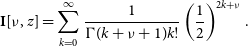 \begin{equation}\textbf{I}[\nu, z]=\sum_{k=0}^{\infty}\frac{1}{\Gamma(k+\nu+1)k!}\left(\frac{1}{2}\right)^{2k+\nu}.\end{equation}
This relation lets us calculate a value of
 $\mu$
to use in our simple visibility model (Equation (7)) and
$\mu$
to use in our simple visibility model (Equation (7)) and
 $\left\langle Z\right\rangle$
of the real observation. For the real observation, we used in comparison,
$\left\langle Z\right\rangle$
of the real observation. For the real observation, we used in comparison,
 $\left\langle Z\right\rangle \approx 2.707\sigma$
, giving us
$\left\langle Z\right\rangle \approx 2.707\sigma$
, giving us
 $\mu\approx 2.495\sigma$
.
$\mu\approx 2.495\sigma$
.
We calculated the mean SNR of the real observation over all frequencies and then produce a series {SNR(f)} whose mean value is equal to the real observation’s such that SNR(f) is proportional to frequency to the
 $-1.59$
, which is derived from fitting a power law distribution to the empirically measured frequency dependence of SNR. The simulated observation with known SNR(f) is directly input into OMNICAL, so that the
$-1.59$
, which is derived from fitting a power law distribution to the empirically measured frequency dependence of SNR. The simulated observation with known SNR(f) is directly input into OMNICAL, so that the
 $\Delta$
values should be mean 1 with any deviations purely caused by noise.
$\Delta$
values should be mean 1 with any deviations purely caused by noise.
We compare
 $\Delta$
’s of a real EoR1 observation (Observation ID: 1163254256) with redundant calibration solutions of the corresponding simulated observation in Figure 2, which shows root mean square (RMS) of redundant calibration solution magnitudes/phases. The RMS is taken across the set of antennas. Clearly, redundant calibration is making changes to the real data at a level significantly larger than might be expected were the data perfectly redundant up to the noise level.
$\Delta$
’s of a real EoR1 observation (Observation ID: 1163254256) with redundant calibration solutions of the corresponding simulated observation in Figure 2, which shows root mean square (RMS) of redundant calibration solution magnitudes/phases. The RMS is taken across the set of antennas. Clearly, redundant calibration is making changes to the real data at a level significantly larger than might be expected were the data perfectly redundant up to the noise level.

Figure 1. The MWA Phase II compact array layout.
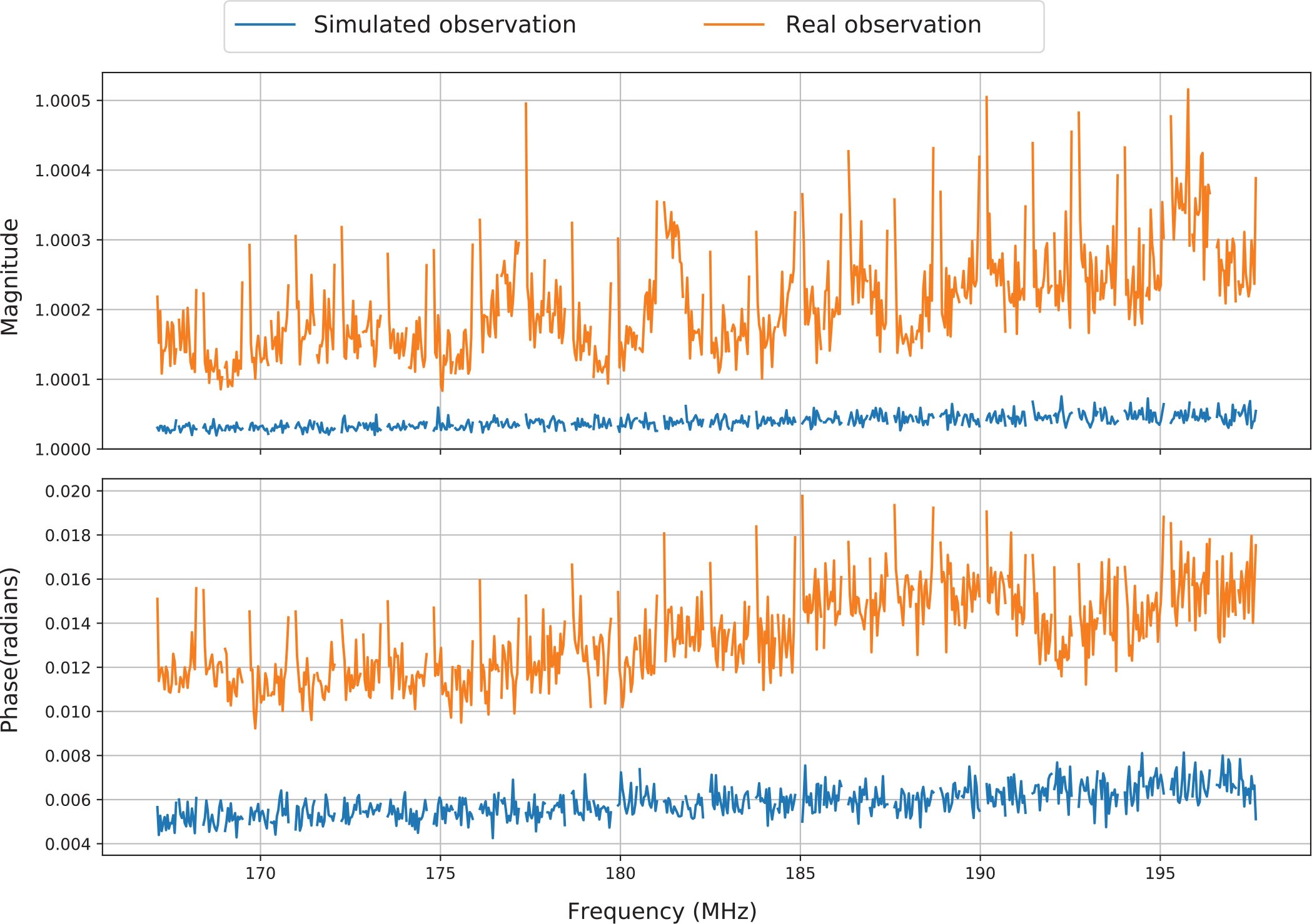
Figure 2. The RMS of redundant calibration solution magnitudes/phases of a real/simulated observation. Orange lines represent the real EoR1 observation and blue lines correspond to the simulated observation, which is constructed to have the same mean noise as the real observation per frequency and the same total SNR averaged over frequencies. In addition, we set the SNR of the simulated observation proportional to frequency to
 $-1.59$
which is similar to the real one. Upper: RMS of redundant calibration solution magnitudes; bottom: RMS of redundant calibration solution phases. We can see that redundant calibration makes changes to the real data beyond just noise.
$-1.59$
which is similar to the real one. Upper: RMS of redundant calibration solution magnitudes; bottom: RMS of redundant calibration solution phases. We can see that redundant calibration makes changes to the real data beyond just noise.
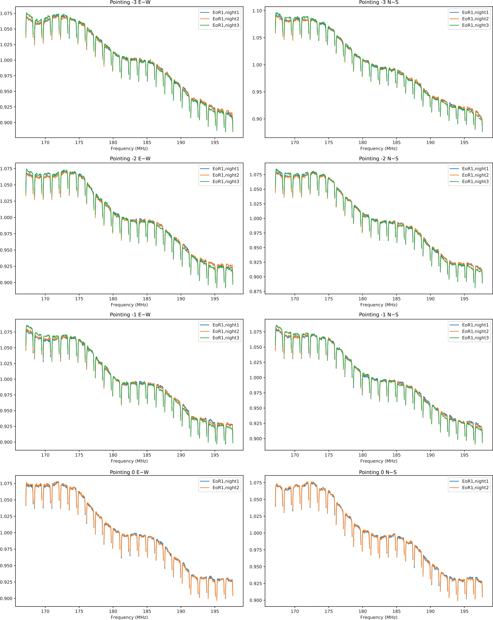
Figure 3. The spectra of FHD solution magnitudes (averaged over antennas and normalised to mean one) of observations with well-matched LSTs over our three EoR1 nights. Blue, orange, and green represent EoR1 night1, night2, and night3, respectively. Two columns correspond to two polarisations and four rows correspond to different pointings. Note that EoR1 night3 pointing 0 is flagged due to ionospheric contamination. The periodic 1.28 MHz scalloping is due to the two-stage Fourier transform used by the MWA correlator. For each 2-min LST-matched data set, the solutions are largely in agreement with only small discrepancies over nights. In general, EoR1 night1 and night2 agree closely, with night3 showing a steeper spectral slope.
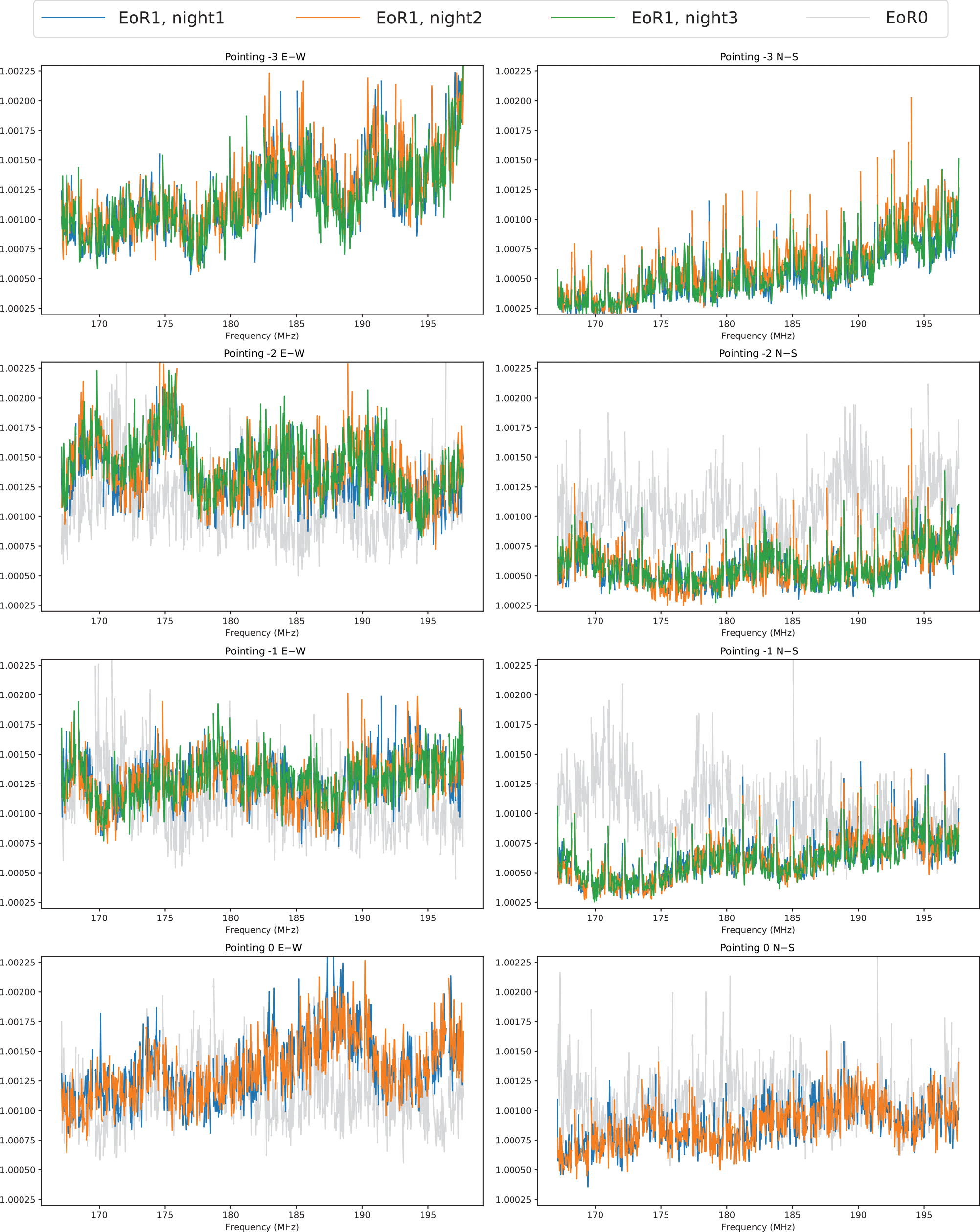
Figure 4. The RMS of magnitudes of
 $\Delta$
’s for observations sampled per pointing per polarisation and per night. EoR1 observations are sampled to have well-matched LSTs over EoR1 nights. We also sampled typical EoR0 observations at pointing −2, −1, and 0. Four different colours denote different nights (see legend at the top of the figure for details). The columns represent the two linear polarisations and each of the four rows correspond to different pointings. We find that
$\Delta$
’s for observations sampled per pointing per polarisation and per night. EoR1 observations are sampled to have well-matched LSTs over EoR1 nights. We also sampled typical EoR0 observations at pointing −2, −1, and 0. Four different colours denote different nights (see legend at the top of the figure for details). The columns represent the two linear polarisations and each of the four rows correspond to different pointings. We find that
 $|\Delta|$
’s are consistent at any pointing over all the EoR1 nights with repeatable frequency structure, and the results from EoR0 observations have different spectral behaviour. It also shows
$|\Delta|$
’s are consistent at any pointing over all the EoR1 nights with repeatable frequency structure, and the results from EoR0 observations have different spectral behaviour. It also shows
 $|\Delta|$
’s for EoR1 observations have bigger values at E–W than at N–S (see further discussion in Section 5).
$|\Delta|$
’s for EoR1 observations have bigger values at E–W than at N–S (see further discussion in Section 5).

Figure 5. Histograms of redundant calibration solutions for EoR1 night1 and night2. Left: 1 and 2D histograms of the magnitudes of redundant calibration solutions for EoR1 night1 and night2. The subplot in the lower left panel is the 2D histogram of the magnitudes of redundant calibration solutions for two simulated data sets with common SNR. Right: 1 and 2D histograms of the phases (in radians) of redundant calibration solutions for EoR1 night1 and night2. The subplot in the lower left panel is the 2D histogram of the phases of redundant calibration solutions for two simulated data sets with common SNR. For 1D histograms, the area between the vertical dashed lines contains 95% of the samples; for 2D histograms, a contour (where the plot transitions from a point-by-point scatter plot to a pixelated density plot) contains
 $1-e^{-2}\approx 84\%$
of the samples. Comparison with the simulated data shows that there is a scatter larger than would be expected from noise, EoR1 night1 and night2 are overall significantly correlated.
$1-e^{-2}\approx 84\%$
of the samples. Comparison with the simulated data shows that there is a scatter larger than would be expected from noise, EoR1 night1 and night2 are overall significantly correlated.
We also investigate the effect of SNR on the result of the simulations. We find that as long as the SNR is held fixed (e.g. increases to the signal strength are offset by increases to the noise), the
 $\Delta$
’s produced by redundant calibration are at the same level. Increasing the SNR does reduce the magnitude of the
$\Delta$
’s produced by redundant calibration are at the same level. Increasing the SNR does reduce the magnitude of the
 $\Delta$
’s, indicating that redundant calibration is indeed affected by noisy data. However, as indicated in Figure 2, the RMS of the
$\Delta$
’s, indicating that redundant calibration is indeed affected by noisy data. However, as indicated in Figure 2, the RMS of the
 $\Delta$
’s for the real data are larger than would be expected from SNR alone.
$\Delta$
’s for the real data are larger than would be expected from SNR alone.
From these results, we can conclude that OMNICAL is responding to real non-redundancy in the data that is above the noise level. Our simulation tells us the expected scale of the
 $\Delta$
’s for a given SNR and perfect redundancy; in the real data, we see
$\Delta$
’s for a given SNR and perfect redundancy; in the real data, we see
 $\Delta$
’s a factor of
$\Delta$
’s a factor of
 ${\sim}3-5$
larger in RMS. This analysis does not, however, tell us the source of the non-redundancy. It might be that the FHD solutions are not completely correct and that OMNICAL is bringing the gains closer to their true values. However, it might be that the instrument itself is non-redundant and OMNICAL is introducing further errors into the gains (since it assumes perfect redundancy). We now continue our analysis of the gain solutions produced by FHD and OMNICAL to see whether the addition of OMNICAL does in fact lead to improvements in our calibration and subsequent analysis.
${\sim}3-5$
larger in RMS. This analysis does not, however, tell us the source of the non-redundancy. It might be that the FHD solutions are not completely correct and that OMNICAL is bringing the gains closer to their true values. However, it might be that the instrument itself is non-redundant and OMNICAL is introducing further errors into the gains (since it assumes perfect redundancy). We now continue our analysis of the gain solutions produced by FHD and OMNICAL to see whether the addition of OMNICAL does in fact lead to improvements in our calibration and subsequent analysis.
4.2. Comparison of calibration solutions
To study the performance of FHD and OMNICAL when applied to actual data, we compare the calibration solutions among the four nights. We perform two distinct analyses: a detailed investigation of the spectral behaviour of four sets (one per pointing that passes the cuts described in Section 2) of calibration solutions from 2-min Local Sidereal Time (LST)-matched data sets (Section 4.2.1) and a study of the repeatability of the calibration solutions across all observations in our data set (Section 4.2.2).
4.2.1. Spectral behaviour of the calibration solutions
Within each pointing, we select one observation per EoR1 night such that the sampled EoR1 observations are at well-matched LSTs. Similar LSTs will result in similar model visibilities generated by FHD. Thus, comparing LST-matched EoR1 observations across nights will test the consistency and repeatability of the calibration techniques.
We also select one observation per pointing from the EoR0 night and compare
 $\Delta's$
with sampled EoR1 observations to explore redundant calibration performance at different EoR fields and a possible sky model dependence. There is obviously no LST accordance between the EoR0 night and EoR1 nights, but the observations chosen are representative.
$\Delta's$
with sampled EoR1 observations to explore redundant calibration performance at different EoR fields and a possible sky model dependence. There is obviously no LST accordance between the EoR0 night and EoR1 nights, but the observations chosen are representative.
We begin by first looking at the FHD sky model calibration solutions for each of our three selected EoR1 observations. We normalise the magnitudes of per-frequency FHD solutions for sampled EoR1 observations to mean 1 and then average over antennas to study the typical spectral structure. Figure 3 shows the magnitude of FHD solutions for sampled observations on the EoR1 nights. For each set of observations with similar LSTs, the solutions are largely in agreement with only small discrepancies over nights. In general, EoR1 nights 1 and 2 agree closely, with night 3 showing a steeper spectral slope.
Comparison of redundant calibration solutions are carried out in a similar way. We look at the spectra of the RMS of the magnitudes of the
 $\Delta$
’s over antennas for each sampled observation. Figure 4 illustrates that
$\Delta$
’s over antennas for each sampled observation. Figure 4 illustrates that
 $|\Delta|$
’s are similarly consistent over all the EoR1 nights with repeatable frequency structure. The grey curve shows the results from an EoR0 observation, which has different spectral behaviour, but no significant difference in overall magnitudes (recall that −3 is a flagged pointing for EoR0 due to Galactic contamination). A comparison of the East–West (E–W) polarisation and the North–South (N–S) polarisation shows that
$|\Delta|$
’s are similarly consistent over all the EoR1 nights with repeatable frequency structure. The grey curve shows the results from an EoR0 observation, which has different spectral behaviour, but no significant difference in overall magnitudes (recall that −3 is a flagged pointing for EoR0 due to Galactic contamination). A comparison of the East–West (E–W) polarisation and the North–South (N–S) polarisation shows that
 $|\Delta|$
’s for EoR1 observations have bigger values at E–W than at N–S. We will return to this point in Section 5, but note that the polarisation dependence of redundant calibration solutions is significantly weaker in the EoR0 observations.
$|\Delta|$
’s for EoR1 observations have bigger values at E–W than at N–S. We will return to this point in Section 5, but note that the polarisation dependence of redundant calibration solutions is significantly weaker in the EoR0 observations.
This result suggests that the spectral structure of our calibration solutions are quite repeatable for the same LST on different nights, but there is a moderate dependence on the pointing. While not shown, we have repeated this analysis for a number of other 2-min LST-matched data and we find the results to be very similar. For redundant calibration solutions, we find a significant difference between the EoR1 and EoR0 fields.
4.2.2. Repeatability of redundant calibration solutions
To make a more robust claim about the night-to-night repeatability of redundant calibration, we pair all the LST-matched redundant calibration
 $\Delta$
’s between two EoR1 nights (up to
$\Delta$
’s between two EoR1 nights (up to
 $10^{10}$
pairs in total, with one pair for each frequency, antenna, and time sample of the data set) and study the correlation between the two nights. Figure 5 shows the results of this study. The top row of two three-panel ‘triangle’ plots show the 1D and 2D histograms of all the redundant calibration
$10^{10}$
pairs in total, with one pair for each frequency, antenna, and time sample of the data set) and study the correlation between the two nights. Figure 5 shows the results of this study. The top row of two three-panel ‘triangle’ plots show the 1D and 2D histograms of all the redundant calibration
 $\Delta$
’s in magnitude (left) and phase (right). Within each triangle, the 1D histograms show the
$\Delta$
’s in magnitude (left) and phase (right). Within each triangle, the 1D histograms show the
 $\Delta$
’s from night1 (top left) and night2 (bottom right); the 2D contour/scatter plot (bottom left) shows the values from night1 plotted against the values from night2. For 1D histograms, the area between the vertical dashed lines contains 95% of the samples; for 2D histograms, a contour (where the plot transitions from a point-by-point scatter plot to a pixelated density plot) contains
$\Delta$
’s from night1 (top left) and night2 (bottom right); the 2D contour/scatter plot (bottom left) shows the values from night1 plotted against the values from night2. For 1D histograms, the area between the vertical dashed lines contains 95% of the samples; for 2D histograms, a contour (where the plot transitions from a point-by-point scatter plot to a pixelated density plot) contains
 $1-e^{-2}\approx 84\%$
of the samples.
$1-e^{-2}\approx 84\%$
of the samples.
The elliptical shape of the 2D histograms, centred on the one-to-one line, suggest that the solutions found on EoR1 night1 and EoR1 night2 are highly correlated. To better assess the significance of this correlation, we perform a similar analysis using two sets of simulated data with common SNR. Since the simulated data (described in Section 4.1) are effectively perfect up to the noise, we expect no correlation in the
 $\Delta$
’s between the two nights (i.e. any change redundant calibration wants to make to the data set is merely a result of fitting noise). The results of this simulation are shown in the bottom two triangle plots in Figure 5. As expected, the 2D histograms are completely circular—meaning there is no correlation in the
$\Delta$
’s between the two nights (i.e. any change redundant calibration wants to make to the data set is merely a result of fitting noise). The results of this simulation are shown in the bottom two triangle plots in Figure 5. As expected, the 2D histograms are completely circular—meaning there is no correlation in the
 $\Delta$
’s between the two simulated nights. The width of these circles also gives us an estimate of the scatter we might expect in perfectly correlated data (because the simulations have an SNR matched to the data). Comparison between real and simulated data shows that the two EoR1 nights are not perfectly correlated up to the noise; rather, the scatter in these plots (effectively, the minor axis of the ellipses) is larger than would be expected from noise alone. However, the overall correlation is quite significant: the redundant calibration solutions for the two nights of data have Pearson’s correlation coefficients of 0.826 (magnitude) and 0.651 (phase), confirming our intuition that redundant calibration is producing largely repeatable results from night to night.
$\Delta$
’s between the two simulated nights. The width of these circles also gives us an estimate of the scatter we might expect in perfectly correlated data (because the simulations have an SNR matched to the data). Comparison between real and simulated data shows that the two EoR1 nights are not perfectly correlated up to the noise; rather, the scatter in these plots (effectively, the minor axis of the ellipses) is larger than would be expected from noise alone. However, the overall correlation is quite significant: the redundant calibration solutions for the two nights of data have Pearson’s correlation coefficients of 0.826 (magnitude) and 0.651 (phase), confirming our intuition that redundant calibration is producing largely repeatable results from night to night.
4.3. Comparison of power spectra
Li et al. (Reference Li2018) and (Reference Li, Pober, Berry and Hazelton2019) evaluated tandem calibration techniques by quantifying the reduction of power in the EoR window (assumed to be due to residual foreground contamination). We apply that formalism in our analyses. To illustrate the difference between the two calibration pipelines, we subtract the PS of data with both FHD and redundant calibration applied from that of the FHD-only applied data in 3D k space. We then select regions of k space where both foregrounds and the periodic contamination from the 1.28-Mhz band structures are minimised and bin in spherical annuli to make 1D PS difference plots versus k. We plot the 1D results as
 $\Delta^2(k) = \frac{k^3}{2\pi^2}P(k)$
to facilitate comparison with the literature. We perform this exercise for both the N–S polarisation and the E–W polarisation and for all four nights. We produce PS using the package Error Propagated Power Spectrum with Interleaved Observed Noise (
$\Delta^2(k) = \frac{k^3}{2\pi^2}P(k)$
to facilitate comparison with the literature. We perform this exercise for both the N–S polarisation and the E–W polarisation and for all four nights. We produce PS using the package Error Propagated Power Spectrum with Interleaved Observed Noise (
 $\varepsilon$
ppsilonFootnote g; Jacobs et al. Reference Jacobs2016; Barry et al. Reference Barry, Beardsley, Byrne, Hazelton, Morales, Pober and Sullivan2019a). In 1D PS difference plots, solid lines represent positive values, that is, the power at that k mode is reduced by the application of redundant calibration to FHD calibrated data, while dashed lines represent negative values. In the EoR window, the former are regarded as ‘improvements’— redundant calibration has lowered the contamination in the region expected to be foreground-free. In Figure 6, we illustrate the modes we select in a 2D PS (although recall the differencing and mode selection takes place in 3D k space). For consistency, we use the same k space selections as used in Li et al. (Reference Li, Pober, Berry and Hazelton2019). The selection gives us a range of
$\varepsilon$
ppsilonFootnote g; Jacobs et al. Reference Jacobs2016; Barry et al. Reference Barry, Beardsley, Byrne, Hazelton, Morales, Pober and Sullivan2019a). In 1D PS difference plots, solid lines represent positive values, that is, the power at that k mode is reduced by the application of redundant calibration to FHD calibrated data, while dashed lines represent negative values. In the EoR window, the former are regarded as ‘improvements’— redundant calibration has lowered the contamination in the region expected to be foreground-free. In Figure 6, we illustrate the modes we select in a 2D PS (although recall the differencing and mode selection takes place in 3D k space). For consistency, we use the same k space selections as used in Li et al. (Reference Li, Pober, Berry and Hazelton2019). The selection gives us a range of
 $|k|$
modes to look at, although we draw particular attention to the modes in 1D PS difference plots where k is about
$|k|$
modes to look at, although we draw particular attention to the modes in 1D PS difference plots where k is about
 $0.15 \sim 0.20\ h\textrm{Mpc}^{-1}$
; these modes have both the largest sensitivity to the EoR signal and come from regions of 2D k space closest to ‘the wedge’, where calibration errors can most easily cause contamination (Morales et al. Reference Morales, Beardsley, Pober, Barry, Hazelton, Jacobs and Sullivan2019).
$0.15 \sim 0.20\ h\textrm{Mpc}^{-1}$
; these modes have both the largest sensitivity to the EoR signal and come from regions of 2D k space closest to ‘the wedge’, where calibration errors can most easily cause contamination (Morales et al. Reference Morales, Beardsley, Pober, Barry, Hazelton, Jacobs and Sullivan2019).
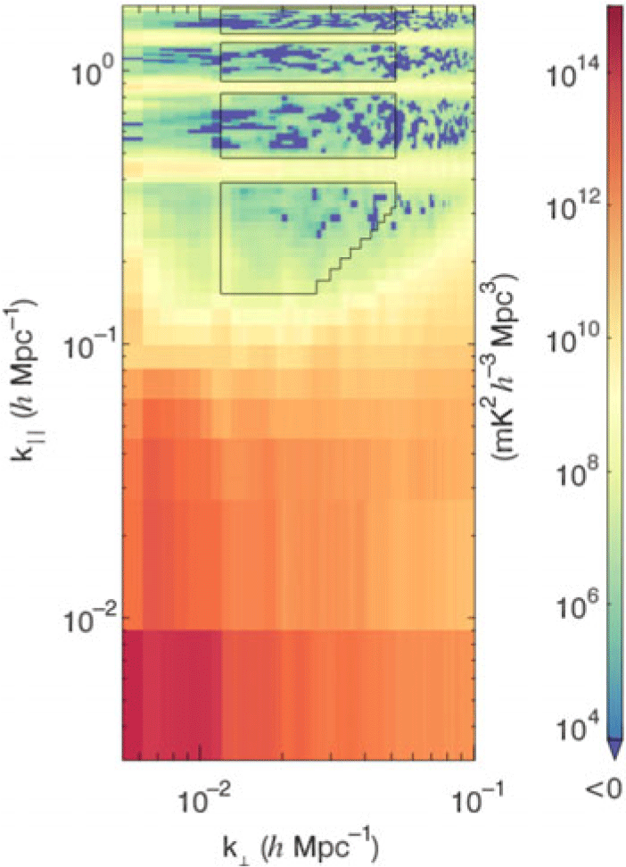
Figure 6. An example for 2D PS plot to highlight modes that will be used for 1D power in k in Figures 7, 8, and 9. To avoid coarse band contamination, we discard 5
 $k_{\parallel}$
bins around the centre of each coarse band mode. Low
$k_{\parallel}$
bins around the centre of each coarse band mode. Low
 $k_\parallel$
values are inside ‘the wedge’ and are therefore not included. In the
$k_\parallel$
values are inside ‘the wedge’ and are therefore not included. In the
 $k_{\perp}$
direction, we keep modes between a lower bound of 12
$k_{\perp}$
direction, we keep modes between a lower bound of 12
 $\lambda$
and an upper bound of 50
$\lambda$
and an upper bound of 50
 $\lambda$
(Li et al. Reference Li, Pober, Berry and Hazelton2019). The cutting is performed in the 3D power spectrum and averaged to one-dimension.
$\lambda$
(Li et al. Reference Li, Pober, Berry and Hazelton2019). The cutting is performed in the 3D power spectrum and averaged to one-dimension.
Figure 7 shows the 1D PS difference for each pointing of the EoR1 nights. For each PS plot, we integrate all observations within the pointing not flagged by our quality metrics. For the E–W polarisation (blue lines), we can see repeatable improvements up to
 $10^4\, \textrm{mK}^2$
for all pointings. In contrast, improvements in the N–S polarisation (orange lines) only appear at the zenith pointing (the fourth row). At the off-zenith pointings (first three rows), we see no significant improvements of PS in the N–S polarisation.
$10^4\, \textrm{mK}^2$
for all pointings. In contrast, improvements in the N–S polarisation (orange lines) only appear at the zenith pointing (the fourth row). At the off-zenith pointings (first three rows), we see no significant improvements of PS in the N–S polarisation.
A 1D pointing-by-pointing PS difference comparison of EoR0 and EoR1 is shown in Figures 8, and 9 shows PS differences after integrating all good pointings for each night. The improvements in the E–W polarisation are seen for all three EoR1 nights, whereas no significant improvements are seen for EoR0 in any pointing or in the integrated PS, consistent with the results of Li et al. (Reference Li, Pober, Berry and Hazelton2019).
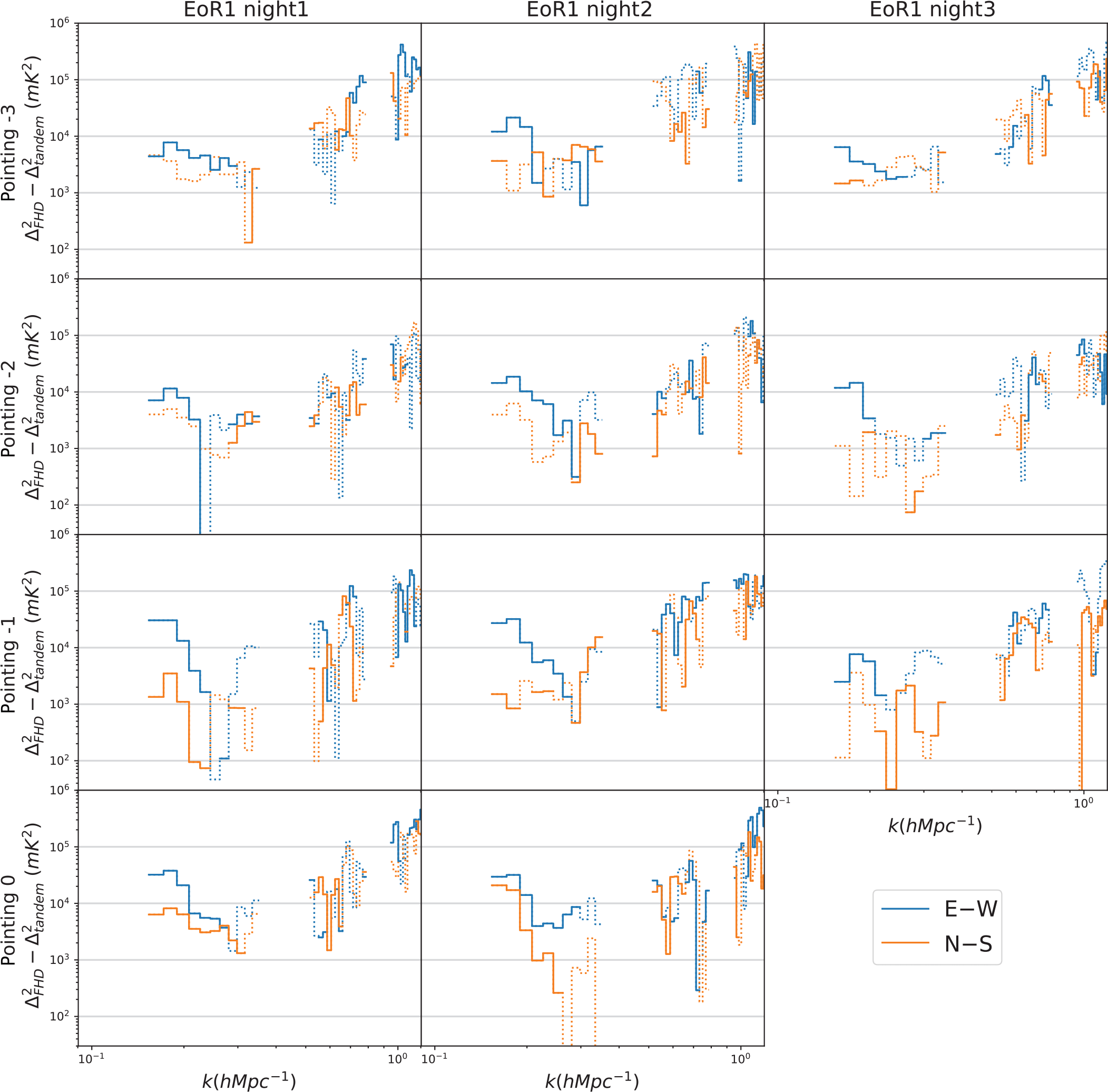
Figure 7. 1D PS difference pointing by pointing for the three EoR1 nights. Solid lines represent k modes where redundant calibration has reduced the overall power, while dotted lines imply a negative reduction in power (i.e. redundant calibration has introduced additional contamination). The three columns correspond to the three nights and the four rows correspond to different pointings. Blue represents the E–W polarisation while orange is N–S. Recall that the night3 zenith pointing is flagged due to ionospheric contamination. For the highest sensitivity modes (
 ${\sim}0.15 - 0.20\ h\textrm{Mpc}^{-1}$
), we can see repeatable improvements up to
${\sim}0.15 - 0.20\ h\textrm{Mpc}^{-1}$
), we can see repeatable improvements up to
 $10^4$
mK
$10^4$
mK
 $^2$
for all pointings in the E–W polarisation (blue lines), while improvements in the N–S polarisation (orange lines) only appear at the zenith pointing (the fourth row).
$^2$
for all pointings in the E–W polarisation (blue lines), while improvements in the N–S polarisation (orange lines) only appear at the zenith pointing (the fourth row).
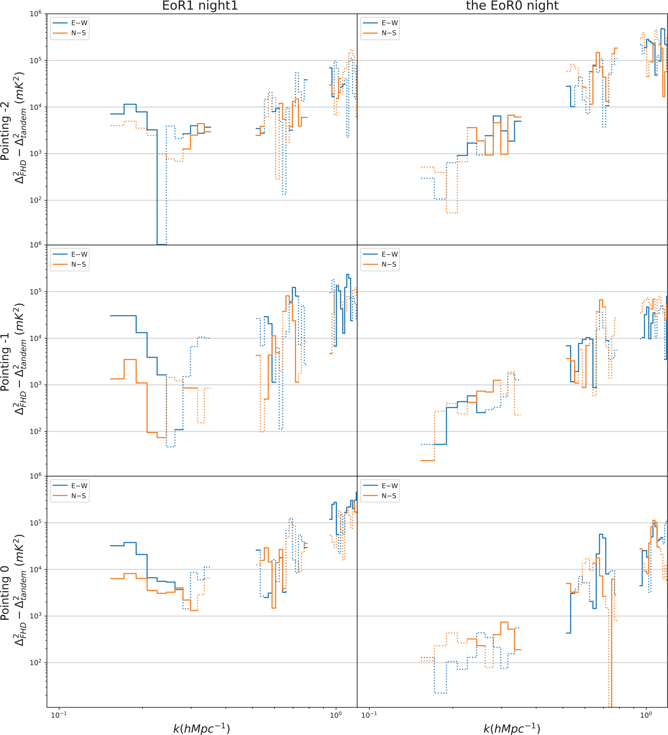
Figure 8. 1D PS difference for EoR1 night1 (left) and the EoR0 night (right). Solid lines represent modes where redundant calibration has reduced the power, while dotted lines imply an increase. Blue represents the E–W polarisation while orange is N–S. The improvements on PS in the E–W polarisation are seen for any pointing at all three EoR1 nights, whereas no significant improvements are seen for any pointing of the EoR0 night. No significant improvements in the N–S polarisation.
In general, when we do see consistent improvements, they are at levels of
 ${\sim}10^3$
to
${\sim}10^3$
to
 $10^4$
mK
$10^4$
mK
 $^2$
. Given the recent measurements of Barry et al. (Reference Barry2019b), Li et al. (Reference Li, Pober, Berry and Hazelton2019), and Trott et al. (Reference Trott2020), which use the MWA to achieve lowest limits of
$^2$
. Given the recent measurements of Barry et al. (Reference Barry2019b), Li et al. (Reference Li, Pober, Berry and Hazelton2019), and Trott et al. (Reference Trott2020), which use the MWA to achieve lowest limits of
 $\Delta^2 < 3.9 \times 10^3\, \textrm{mK}^2$
,
$\Delta^2 < 3.9 \times 10^3\, \textrm{mK}^2$
,
 $\Delta^2 < 2.39 \times 10^3\, \textrm{mK}^2$
, and
$\Delta^2 < 2.39 \times 10^3\, \textrm{mK}^2$
, and
 $\Delta^2 < 1.8 \times 10^3\, \textrm{mK}^2$
, respectively, we can see improvements of this scale can be significant.
$\Delta^2 < 1.8 \times 10^3\, \textrm{mK}^2$
, respectively, we can see improvements of this scale can be significant.
5. Discussion
In Section 4, we presented analyses looking at both calibration solutions and 1D PS differences. In this section, we will further discuss two key aspects of our results: the comparison of the EoR1 and EoR0 results and the polarisation dependence of redundant calibration’s improvements in the PS of EoR1.
5.1. Comparison of EoR1 and EoR0
The noise simulations (Section 4.1) and general repeatability of both the gain solutions (Section 4.2) and the PS improvements (Section 4.3) across the three nights of EoR1 give us significant confidence that redundant calibration is indeed constraining real information about the telescope. It is then interesting to ask why we see no significant PS improvements in our EoR0 analysis (consistent with the results of Li et al. Reference Li, Pober, Berry and Hazelton2019).
The biggest difference between the two fields is the distribution of flux density on the sky. EoR0 has no significant bright or extended sources (Carroll et al. Reference Carroll2016) and as such is well modelled by the GLEAM catalogue. For EoR1, our sky model is likely not as accurate as the EoR0 due to the presence of Fornax A (see Figure 10) near the centre of the field. GLEAM does not include a Fornax A model (Hurley-Walker et al. Reference Hurley-Walker2016) itself; ours is produced directly from Phase I EoR observations using the techniques of Carroll et al. (Reference Carroll2016). Figure 11 shows the residual images of EoR1 after our sky model has been subtracted; we return to the polarisation properties of this image in our discussion in Section 5.2, but we generally see a negative feature at the position of Fornax A in the lower right of the image—suggesting our model has an excess of flux density compared to the data. However, we emphasise that our Fornax A model is by no means ‘bad’; the post-subtraction residuals seen in Figure 11 are at the percent level compared to the source itself. Line et al. (Reference Line2020) recently produced a new model for Fornax A using shapelets (which, at present, cannot be used by the FHD code), but when subtracted from MWA data, the residuals are at comparable level to those seen here (c.f. their Figure 9).

Figure 9. 1D PS difference of the full night for all nights. Solid lines represent a reduction of power from redundant calibration, while dotted lines imply an increase. Upper left: full night residual PS at EoR1 night1; bottom left: full night residual PS at EoR1 night2; upper right: full night residual PS at EoR1 night3; bottom right: full night residual PS at the EoR0 night. Blue represents polarisation E–W while orange represents polarisation N–S. The improvements in the integrated, E–W polarisation PS are seen for all three EoR1 nights, whereas no significant improvements are seen for EoR0. Neither field shows significant improvements in the N–S polarisation.
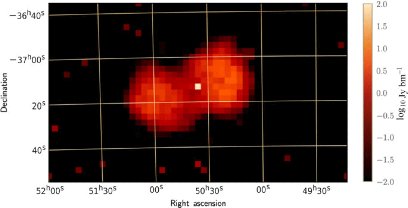
Figure 10. The extended source model used for Fornax A produced using the techniques of Carroll et al. Reference Carroll2016. This image is at 150 MHz and has a peak flux density of
 $\sim$
313 Jy. A total of 1 925 components are used for this model.
$\sim$
313 Jy. A total of 1 925 components are used for this model.
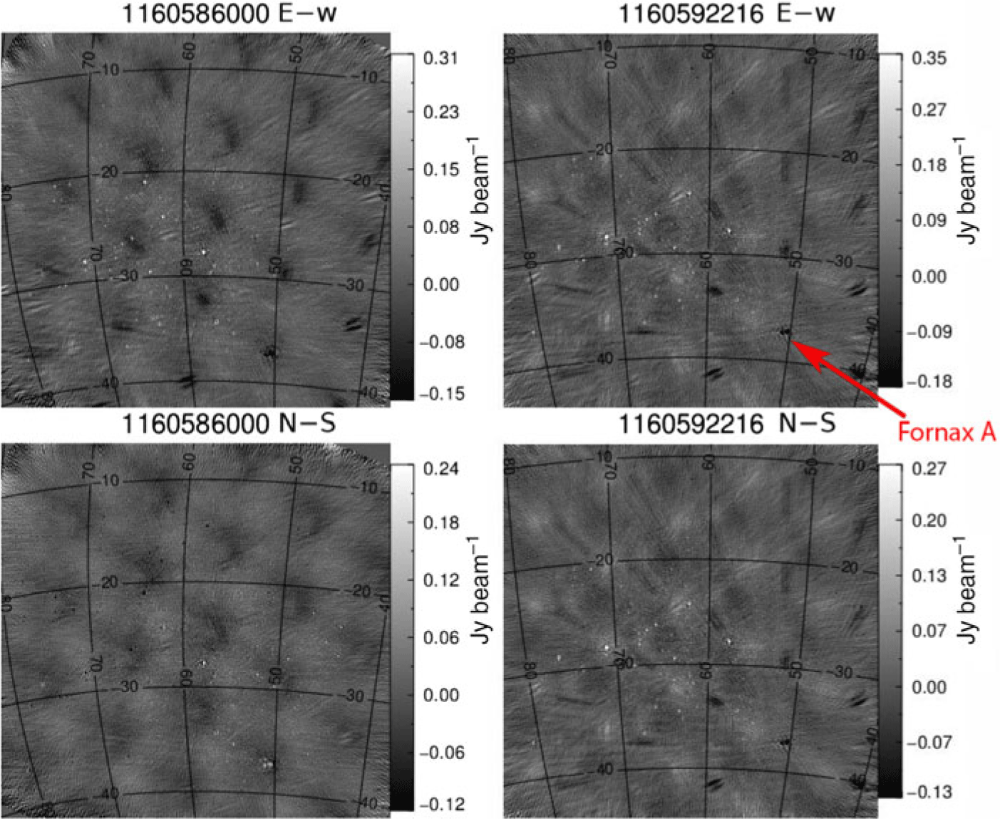
Figure 11. Residual images for both the E–W and N–S polarisation of a zenith observation (observation id: 1160592216) and an off-zenith observation (observation id: 1160586000). Upper left: residual image for E–W off-zenith; bottom left: residual image for N–S off-zenith; upper right: residual image for E–W zenith; bottom right: residual image for N–S zenith.
The fact that Fornax A is so difficult to model leads to interesting conclusions about the role of redundant calibration in the EoR1 field. If FHD produces calibration solutions with frequency-dependent errors driven by sky model incompleteness (as suggested in Barry et al. Reference Barry, Hazelton, Sullivan, Morales and Pober2016), then we will expect sky-based calibration to perform relatively worse on EoR1; redundant calibration, to the extent that it is sky-model-independent, will therefore have a more significant effect. Figure 4 indeed shows that redundant calibration solutions behave differently between EoR1 and EoR0, consistent with the idea that the model errors introduced in FHD are significantly different. In fact, even for the observations at the same pointing but separated by several minutes, redundant calibration solutions can have significantly different spectra, which implies that FHD calibration is quite sensitive to LST. Our results therefore suggest that redundant calibration techniques can still play a role mitigating sky model errors in calibration—especially for fields with difficult, extended sources—even though sky model errors will still enter through the degenerate parameters (Byrne et al. Reference Byrne2019).
5.2. Polarisation dependence of redundant calibration performance
In Section 4.3, we saw that the PS improvements from redundant calibration in the EoR1 data were strongly polarisation-dependent: for the E–W polarisation, we saw substantive and consistent improvement at all pointings; for the N–S polarisation, there were no improvements at off-zenith pointings and, while there was improvement at the zenith pointing, it was less than that of the E–W polarisation.
To explain the strong polarisation dependence in redundant calibration’s impact on the PS, we picked one zenith observation and one off-zenith observation of EoR1 night1 and investigated their FHD products. In particular, we looked at the residual images for both polarisations, which are generated from calibrated, residual visibilities, as shown in Figure 11. As mentioned in Section 5.1, Fornax A is located near the centre of EoR1. Looking at residual images for both polarisations from an EoR1 zenith observation (observation ID 1160592216, right-hand column) leads us to conclude that our Fornax A model contains too much flux density, leading to the negative hole at RA
 $50^{\circ}$
, Dec
$50^{\circ}$
, Dec
 $-37^{\circ}$
. This error clearly produces many other artefacts in the image, including a strong set of negative features associated with sidelobes of Fornax A and a general miscalibration and undersubtraction of the numerous other points sources in the field.
$-37^{\circ}$
. This error clearly produces many other artefacts in the image, including a strong set of negative features associated with sidelobes of Fornax A and a general miscalibration and undersubtraction of the numerous other points sources in the field.
This pattern is seen in both polarisations of the zenith pointing—both of which are improved by redundant calibration. We also see the oversubtraction of Fornax A and undersubtraction of other sources in the E–W residual image from an EoR1 off-zenith observation (observation ID 1160586000, left-hand column). This is consistent with the fact that redundant calibration improves the E–W PS of an off-zenith observation. However, the N–S residual image looks quite different. Instead, we see an undersubtraction of Fornax A and oversubtraction of many point sources in the upper left of the image. The sidelobes of Fornax A are also significantly mitigated.
The most likely explanation for this effect is an error in our model of the tile primary beam. For any given pointing, the primary beam differs between the two linear polarisations. At zenith, this is simply because the dipoles for detecting one polarisation are rotated
 $90{^\circ}$
from each other (and the beam pattern of a dipole—and therefore our tiles as well—is not symmetric under a
$90{^\circ}$
from each other (and the beam pattern of a dipole—and therefore our tiles as well—is not symmetric under a
 $90{^\circ}$
rotation). For pointings off-zenith, the difference between the two polarisations can be even more complicated, as the projection of the tile towards the pointing centre can make the effective spacing between one polarisation’s dipoles appear foreshortened by a different amount than the other. In general, our beam models are best for zenith but become less accurate for other pointings.
$90{^\circ}$
rotation). For pointings off-zenith, the difference between the two polarisations can be even more complicated, as the projection of the tile towards the pointing centre can make the effective spacing between one polarisation’s dipoles appear foreshortened by a different amount than the other. In general, our beam models are best for zenith but become less accurate for other pointings.
The key impact for this work is that the beam model error made at the position of a specific source (e.g. Fornax A) will not be the same in the two polarisations. What we find is that, in the N–S off-zenith pointing, a fortuitous combination of error in the model of Fornax A itself and the polarisation-dependent beam model error reduces the total level of sky model error. In the E–W polarisation and the N–S zenith pointing, the model error in Fornax A is the dominant source of error in our calibration solutions; such an error can be mitigated by redundant calibration, explaining why we see PS improvements with OMNICAL in all the observations except the N–S off-zenith pointings. This explanation is consistent with Figure 4, where the
 $|\Delta|$
’s at the N-=S polarisation are smaller than those at the E–W polarisation, particularly for off-zenith pointings.
$|\Delta|$
’s at the N-=S polarisation are smaller than those at the E–W polarisation, particularly for off-zenith pointings.
6. Conclusions
In this paper, we studied the performance of tandem redundant and sky-based calibration in MWA Phase II data analysis in the EoR1 field. Using FHD and OMNICAL in tandem, we calibrated and processed three nights of EoR1 observations, as well as one night of EoR for comparison with Li et al. (Reference Li, Pober, Berry and Hazelton2019). We performed a simulation to study redundant calibration’s performance on fitting noise. We also analyzed calibration solutions and improvements in PS. Redundant calibration solutions were found to have night-to-night consistency and resulted in repeatable, substantive improvements in the PS of the EoR1 field. We also saw the strong polarisation dependence of redundant calibration’s impact on the PS. Our principal findings are as follows:
Redundant calibration gives non-negligible gain solutions. Our simulation shows that redundant calibration produces changes to the FHD sky-based gain solutions that are larger than would be expected if it were simply fitting to noise.
Redundant calibration’s performance is repeatable. In our night-to-night comparisons, redundant calibration solutions and PS improvements are repeatable over the same range of LSTs.
Redundant calibration brings about substantive improvements in EoR1. Generally, redundant calibration makes bigger improvements in the EoR1 PS than in EoR0 PS, including changes up to
 $10^4\ \textrm{mK}^2$
in the E–W polarisation.
$10^4\ \textrm{mK}^2$
in the E–W polarisation.
Redundant calibration brings about larger improvements when the sky and beam model of FHD is worse. Both the explanation for the bigger improvements in EoR1 PS than in EoR0 PS and our discussion for why we see the strong polarisation dependence in redundant calibration’s impact on PS tell us that when sky model incompleteness errors most affect sky-based calibration, redundant calibration can result in larger improvements in the PS.
These findings suggest that redundant calibration can continue to play an important role in 21-cm cosmology analysis going forward. While the results from EoR0 suggest that with a good enough sky model for sky-based calibration, redundant calibration becomes ineffective, we note that the limits from Barry et al. (Reference Barry2019b), Li et al. (Reference Li, Pober, Berry and Hazelton2019), and Trott et al. (Reference Trott2020) are all still one to two orders of magnitude above any plausible EoR signal models. Therefore, all we can conclude is that the errors that can be mitigated by redundant calibration are not the dominant source of error in those works. The present work shows that redundant calibration can indeed mitigate some level of sky-based calibration error and so it may continue to yield PS improvements once the current leading sources of systematic errors are mitigated. To end on a note of caution, however, we should be prepared for the possibility that true non-redundancy in the array may become a real problem for redundant calibration and that, once lower PS levels are reached, the inclusion of redundant calibration algorithms may introduce more errors than they mitigate. Research into new approaches that can balance sky-based and redundancy-based errors (e.g. Sievers Reference Sievers2017 and Byrne et al. Reference Byrne, Morales, Hazelton and Wilensky2020) is therefore of particular interest.
Acknowledgements
ZZ, JCP, and WL would like to acknowledge the support from NSF grant #1613040. BJH and MFM would like to acknowledge the support from NSF grants #1506024, #1613855, and #1643011. WL would like to acknowledge the Galkin Foundation Fellowship. KT is partially supported by Grand-in-Aid from the Ministry of Education, Culture, Sports, and Science and Technology (MEXT) of Japan, No. 15H05896, 16H05999 and 17H01110, and Bilateral Joint Research Projects of JSPS. This scientific work makes use of the Murchison Radio-astronomy Observatory, operated by CSIRO. We acknowledge the Wajarri Yamatji people as the traditional owners of the Observatory site. Support for the operation of the MWA is provided by the Australian Government (NCRIS), under a contract to Curtin University administered by Astronomy Australia Limited. We acknowledge the Pawsey Supercomputing Centre which is supported by the Western Australian and Australian Governments. Parts of this research were supported by the Australian Research Council Centre of Excellence for All Sky Astrophysics in 3 Dimensions (ASTRO 3D), through project number CE170100013. CMT is supported by an ARC Future Fellowship under grant FT180100321. The International Centre for Radio Astronomy Research (ICRAR) is a Joint Venture of Curtin University and The University of Western Australia, funded by the Western Australian State government. The MWA Phase II upgrade project was supported by Australian Research Council LIEF grant LE160100031 and the Dunlap Institute for Astronomy and Astrophysics at the University of Toronto. This research was conducted using computation resources and services at the Center for Computation and Visualization, Brown University.


