


In memoriam of Sergio Dain [1970-2016], who gave the first proof of the trace-free Korn's inequality on bounded Lipschitz domains.
1. Introduction
Korn-type inequalities are crucial for a priori estimates in linear elasticity and fluid mechanics. They allow to bound the  $L^{p}$-norm of the gradient
  $\operatorname {D}\hspace {-1pt} u$ in terms of the symmetric gradient, i.e. Korn's first inequality states
 \begin{equation} \exists\, c > 0 \ \forall\, u\in W^{1,p}_{0}(\Omega,\mathbb{R}^{n}): \quad \lVert{\operatorname{D}\hspace{-1pt} u}\rVert_{L^{p}(\Omega,\mathbb{R}^{n\times n})}\leq c\, \lVert{\operatorname{sym} \operatorname{D}\hspace{-1pt} u}\rVert_{L^{p}(\Omega,\mathbb{R}^{n\times n})}. \end{equation}
Generalizations to many different settings have been obtained in the literature, including the geometrically nonlinear counterpart [Reference Faraco and Zhong23, Reference Friesecke, James and Müller24, Reference Lewicka and Müller39], mixed growth conditions [Reference Conti, Dolzmann and Müller15], incompatible fields (also with dislocations) [Reference Bauer, Neff, Pauly and Starke6, Reference Lewintan, Müller and Neff40–Reference Lewintan and Neff43, Reference Müller, Scardia and Zeppieri48, Reference Neff, Pauly and Witsch55–Reference Neff, Pauly and Witsch58], as well as the case of non-constant coefficients [Reference Lankeit, Neff and Pauly37, Reference Neff50, Reference Neff and Pompe59, Reference Pompe62] and on Riemannian manifolds [Reference Chen and Jost9]. In this paper we focus on their improvement towards the trace-free case:
 \begin{equation} \exists\ c > 0 \ \forall\, u\in W^{1,p}_{0}(\Omega,\mathbb{R}^{n}): \quad \lVert{\operatorname{D}\hspace{-1pt} u}\rVert_{L^{p}(\Omega,\mathbb{R}^{n\times n})}\leq c\, \lVert{\operatorname{dev}_n\operatorname{sym} \operatorname{D}\hspace{-1pt} u}\rVert_{L^{p}(\Omega,\mathbb{R}^{n\times n})}, \end{equation}
where  $\operatorname {dev}_n X : = X -\frac 1n\operatorname {tr}(X)\cdot {\mathbb{1}}$ denotes the deviatoric (trace-free) part of the square matrix
  $X$. Note in passing that (1.2) implies (1.1).
There exist many different proofs and generalizations of the trace-free classical Korn's inequality in the literature, see [Reference Reshetnyak63, theorem 2] but also [Reference Bauer, Neff, Pauly and Starke6, Reference Dain17, Reference Fuchs and Schirra27, Reference Jeong and Neff33, Reference Reshetnyak64, Reference Schirra65] as well as [Reference Wang67] for trace-free Korn's inequalities in pseudo-Euclidean space and [Reference Dain17, Reference Holst, Kommemi and Nagy32] for trace-free Korn inequalities on manifolds, [Reference Breit, Cianchi and Diening8, Reference Fuchs25] for trace-free Korn inequalities in Orlicz spaces and [Reference Ding and Li18, Reference López-García45] for weighted trace-free Korn inequalities in Hölder and John domains. Such coercive inequalities found application in micro-polar Cosserat-type models [Reference Fuchs and Schirra27, Reference Jeong and Neff33, Reference Jeong, Ramézani, Münch and Neff34, Reference Neff, Jeong and Ramezani49] and general relativity [Reference Dain17]. On the other hand, corresponding trace-free coercive inequalities for incompatible tensor fields are useful in infinitesimal gradient plasticity as well as in linear relaxed micromorphic elasticity, see [Reference Ghiba, Neff, Madeo and Múnch31, Reference Neff, Ghiba, Lazar and Madeo51] but also [Reference Bauer, Neff, Pauly and Starke6, sec. 7] and the references contained therein.
Notably, in case  $n=2$, the condition
  $\operatorname {dev}_2\operatorname {sym}\operatorname {D}\hspace {-1pt} u\equiv 0$ becomes the system of Cauchy-Riemann equations, so that the corresponding kernel is infinite-dimensional and an adequate quantitative version of the trace-free classical Korn's inequality does not hold true. Nevertheless, in [Reference Fuchs and Schirra27] it is proved that
 \begin{equation} \lVert{\operatorname{D}\hspace{-1pt} u}\rVert_{L^{p}(\Omega,\mathbb{R}^{2\times 2})}\le c\,\lVert{\operatorname{dev}_2\operatorname{sym}\operatorname{D}\hspace{-1pt} u}\rVert_{L^{p}(\Omega,\mathbb{R}^{2\times 2})}\end{equation}
holds for each  $u\in W^{1,p}_0(\Omega ,\mathbb {R}^{2})$,Footnote 1 but, again, this result ceases to be valid if the Dirichlet conditions are prescribed only on a part of the boundary, cf. the counterexample in [Reference Bauer, Neff, Pauly and Starke6, sec. 6.6].
Korn-type inequalities fail for the limiting cases  $p=1$ and
  $p=\infty$. Indeed, from the counterexamples traced back in [Reference Conti, Faraco and Maggi16, Reference de Leeuw and Mirkil38, Reference Mityagin47, Reference Ornstein61] it follows that
  $\int _\Omega \lvert {\operatorname {sym}\operatorname {D}\hspace {-1pt} u}\rvert \mathrm {d}{x}$ does not dominate each quantity
  $\int _\Omega \lvert {\partial _i u_j}\rvert \mathrm {d}{x}$ for any vector field
  $u\in W^{1,1}_0(\Omega ,\mathbb {R}^{n})$. Hence, also trace-free versions fail for
  $p=1$ and
  $p=\infty$. On the other hand, Poincaré-type inequalities estimating certain integral norms of the deformation
  $u$ in terms of the total variation of the symmetric strain tensor
  $\operatorname {sym}\operatorname {D}\hspace {-1pt} u$ are still valid. In particular, for Poincaré-type inequalities for functions of bounded deformation involving the deviatoric part of the symmetric gradient we refer to [Reference Fuchs and Repin26].
The classical Korn's inequalities need compatibility, i.e. a gradient  $\operatorname {D}\hspace {-1pt} u$; giving up the compatibility necessitates controlling the distance of
  $P$ to a gradient by adding the incompatibility measure (the dislocation density tensor)
  $\operatorname {Curl} P$. We showed in [Reference Lewintan and Neff43] the following quantitative version of Korn's inequality for incompatible tensor fields
  $P\in W^{1,p}(\operatorname {Curl}; \Omega ,\mathbb {R}^{3\times 3})$:
 \begin{equation} \inf_{\widetilde{A}\in\mathfrak{so}(3)}\lVert{P-\widetilde{A}}\rVert_{L^{p}(\Omega,\mathbb{R}^{3\times 3})} \leq c\,\left(\lVert{ \operatorname{sym} P }\rVert_{L^{p}(\Omega,\mathbb{R}^{3\times 3})}+ \lVert{ \operatorname{Curl} P }\rVert_{L^{p}(\Omega,\mathbb{R}^{3\times 3})}\right).\end{equation}
Note that the constant skew-symmetric matrix fields (restricted to  $\Omega$) represent the elements from the kernel of the right-hand side of (1.4). For compatible
  $P=\operatorname {D}\hspace {-1pt} u$ recover from (1.4) the quantitative version of the classical Korn's inequality, namely for
  $u\in W^{1,p}(\Omega ,\mathbb {R}^{3})$:
 \begin{equation} \inf_{\widetilde{A}\in\mathfrak{so}(3)}\lVert{\operatorname{D}\hspace{-1pt} u- \widetilde{A}}\rVert_{L^{p}(\Omega,\mathbb{R}^{3\times 3})}\leq c\, \lVert{\operatorname{sym} \operatorname{D}\hspace{-1pt} u}\rVert_{L^{p}(\Omega,\mathbb{R}^{3\times 3})}\end{equation}
and for skew-symmetric matrix fields  $P=A\in \mathfrak {so}(3)$ the corresponding Poincaré inequality for squared skew-symmetric matrix fields
  $A\in W^{1,p}(\Omega ,\mathfrak {so}(3))$ (and thus for vectors in
  $\mathbb {R}^{3}$):
 \begin{equation} \inf_{\widetilde{A}\in\mathfrak{so}(3)}\lVert{A-\widetilde{A} }\rVert_{L^{p}(\Omega,\mathbb{R}^{3\times 3})} \leq c\, \lVert{\operatorname{Curl} A}\rVert_{L^{p}(\Omega,\mathbb{R}^{3\times 3})} \le \tilde{c}\, \lVert{\operatorname{D}\hspace{-1pt} A}\rVert_{L^{p}(\Omega,\mathbb{R}^{ {3\times 3^{2}}})}, \end{equation}
where in the last step we have used that  $\operatorname {Curl}$ consists of linear combinations from
  $\operatorname {D}\hspace {-1pt}$. Interestingly, for skew-symmetric
  $A$ also the converse is true, more precisely, the entries of
  $\operatorname {D}\hspace {-1pt} A$ are linear combinations of the entries from
  $\operatorname {Curl} A$, cf. e.g. [Reference Lewintan and Neff43, Cor. 2.3]:
 \begin{equation} \operatorname{D}\hspace{-1pt} A = L(\operatorname{Curl} A) \qquad \text{for skew-symmetric } A, \end{equation}
where  $L(.)$ denotes a corresponding linear operator with constant coefficients, not necessarily the same in any two places in the present paper. In fact, the mentioned results also hold in higher dimensions
  $n>3$, see [Reference Lewintan and Neff42] and the discussion contained therein. In our proof of (1.4) we were highly inspired by a proof of (1.5) advocated by P. G. Ciarlet and his collaborators [Reference Ciarlet10–Reference Ciarlet, Malin and Mardare14, Reference Duvaut and Lions19, Reference Geymonat and Suquet29], which uses the Lions lemma resp. Nečas estimate, the compact embedding
  $W^{1,p}\subset \!\subset L^{p}$ and the representation of the second distributional derivatives of the displacement
  $u$ by a linear combination of the first derivatives of the symmetrized gradient
  $\operatorname {D}\hspace {-1pt} u$:
 \begin{equation} \operatorname{D}\hspace{-1pt}^{2} u = L(\operatorname{D}\hspace{-1pt}\, \operatorname{sym} \operatorname{D}\hspace{-1pt} u). \end{equation}
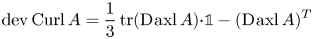
It is worth mentioning that the role of the latter ingredient (1.8) was taken over by (1.7) in our proof of (1.4) in [Reference Lewintan and Neff43] resp. [Reference Lewintan and Neff42]. In  $n=3$ dimensions the relation (1.7) is an easy consequence of the so called Nye's formula [Reference Nye60, eq. (7)]:
 \begin{equation} \operatorname{Curl} A = \operatorname{tr}(\operatorname{D}\hspace{-1pt} \operatorname{axl} A)\cdot {\mathbb{1}}- (\operatorname{D}\hspace{-1pt} \operatorname{axl} A)^{T},\end{equation}
resp.
 \begin{equation} \operatorname{D}\hspace{-1pt} \operatorname{axl} A = \frac 12 \,\operatorname{tr}(\operatorname{Curl} A) \cdot {\mathbb{1}} - (\operatorname{Curl} A)^{T}, \end{equation}
where we identify the vectorspace of skew-symmetric matrices  $\mathfrak {so}(3)$ and
  $\mathbb {R}^{3}$ via
  $\operatorname {axl}:\mathfrak {so}(3)\to \mathbb {R}^{3}$ which is defined by the cross product:
 \begin{equation} A\, b = : \operatorname{axl}(A)\times b \quad \forall\, b\in\mathbb{R}^{3}, \end{equation}
and associates with a skew-symmetric matrix  $A\in \mathfrak {so}(3)$ the vector
  $\operatorname {axl} A : = (-A_{23},A_{13},-A_{12})^{T}$. The relation (1.9a) admits moreover a counterpart on the group of orthogonal matrices
  $\operatorname {O}(3)$ and even in higher spatial dimensions, see [Reference Neff and Münch54]. In fact, Nye's formula is (formally) a consequence of the following algebraic identity:
 \begin{equation} (\operatorname{Anti} a)\times b = b \otimes a -\big\langle{b},{a}\big\rangle {\cdot} {\mathbb{1}} \qquad \forall\, a,b\in\mathbb{R}^{3}, \end{equation}
where the vector product of a matrix and a vector is to be seen row-wise and  $\operatorname {Anti}: \mathbb {R}^{3}\to \mathfrak {so}(3)$ is the inverse of
  $\operatorname {axl}$. Despite the absence of the simple algebraic relations in the higher dimensional case a corresponding relation to (1.7) also holds true in
  $n>3$, see e.g. [Reference Lewintan and Neff42].
Moreover, the kernel in quantitative versions of Korn's inequalities is killed by corresponding boundary conditions, namely by a vanishing trace condition  $u_{|_{\partial \Omega }}=0$ in the case of (1.5) and (1.6) and by a vanishing tangential trace condition
  $P\times \nu ~_{|_{\partial \Omega }}=0$ in the general case (1.4), cf. [Reference Lewintan and Neff42, Reference Lewintan and Neff43].
The objective of the present paper is to improve on inequality (1.4) by showing that it already suffices to consider the deviatoric (trace-free) parts on the right-hand side, hence, further contributing to the problems proposed in [Reference Neff, Pauly and Witsch58]. More precisely, the main results are
Theorem 1 Let  $\Omega \subset \mathbb {R}^{3}$ be a bounded Lipschitz domain and
  $1< p<\infty$. There exists a constant
  $c=c(p,\Omega )>0$ such that for all
  $P\in L^{p}(\Omega ,\mathbb {R}^{3\times 3})$ we have
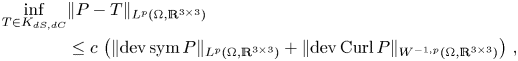 \begin{align} \inf_{T\in K_{dS,dC}}&\lVert{P-T}\rVert_{L^{p}(\Omega,\mathbb{R}^{3\times 3})}\nonumber\\ &\leq c\,\left(\lVert{\operatorname{dev} \operatorname{sym} P }\rVert_{L^{p}(\Omega,\mathbb{R}^{3\times 3})}+ \lVert{\operatorname{dev}\operatorname{Curl} P }\rVert_{W^{{-}1,p}(\Omega,\mathbb{R}^{3\times 3})}\right)\,, \end{align}
where  $\operatorname {dev} X : = X -\frac 13 \operatorname {tr}(X) {\cdot }{\mathbb{1}}$ denotes the deviatoric part of a square tensor
  $X\in \mathbb {R}^{3\times 3}$ and
  $K_{dS,dC}$ represent the kernel of the right-hand side and is given by
 \begin{align} K_{dS,dC} &= \{T:\Omega\to\mathbb{R}^{3\times 3}\mid T(x)=\operatorname{Anti}\big(\widetilde{A}\,x+\beta\, x+b \big)+\big(\big\langle{\operatorname{axl}\widetilde{A}},{x}\big\rangle+\gamma \big) {\cdot}{\mathbb{1}}, \nonumber\\ &\quad \widetilde{A}\in\mathfrak{so}(3), b\in\mathbb{R}^{3}, \beta,\gamma\in\mathbb{R}\}. \end{align}
 By killing the kernel with tangential trace conditions (note that  $\operatorname {dev}(P\times \nu )=0$ iff
  $P\times \nu =0$) we arrive at the following Korn's first type inequality
Theorem 2 Let  $\Omega \subset \mathbb {R}^{3}$ be a bounded Lipschitz domain and
  $1< p<\infty$. There exists a constant
  $c=c(p,\Omega )>0$ such that we have
 \begin{equation} \lVert{ P }\rVert_{L^{p}(\Omega,\mathbb{R}^{3\times 3})}\leq c\,\left(\lVert{\operatorname{dev} \operatorname{sym} P }\rVert_{L^{p}(\Omega,\mathbb{R}^{3\times 3})}+ \lVert{ \operatorname{dev}\operatorname{Curl} P }\rVert_{L^{p}(\Omega,\mathbb{R}^{3\times 3})}\right)\end{equation}
for all
 \begin{align*} P&\in W^{1,p}_0(\operatorname{Curl}; \Omega,\mathbb{R}^{3\times 3})\\ &\quad: = \{P\in L^{p}(\Omega,\mathbb{R}^{3\times 3})\mid \operatorname{Curl} P\in L^{p}(\Omega,\mathbb{R}^{3\times 3}), \ P\times\nu\equiv 0 \text{ on }\partial\Omega\}. \end{align*}
The appearance of the term  $\operatorname {dev}\operatorname {Curl} P$ on the right-hand side of (1.14) would suggest to consider
  $p$-integrable tensor fields
  $P$ with ‘only’
  $p$-integrable
  $\operatorname {dev}\operatorname {Curl} P$. However, this would not lead to a new Banach space, since we show that for all
  $m\in \mathbb {Z}$ it holds that
 \begin{equation} \operatorname{Curl} P \in W^{m,p}(\Omega,\mathbb{R}^{3\times 3}) \quad \Leftrightarrow\quad \operatorname{dev}\operatorname{Curl} P \in W^{m,p}(\Omega,\mathbb{R}^{3\times 3}).\end{equation}
 The estimate (1.14) generalizes the corresponding result in [Reference Bauer, Neff, Pauly and Starke6] from the  $L^{2}$-setting to the
  $L^{p}$-setting, whereas the trace-free second type inequality (1.12) is completely new. Generalizations to different right-hand sides and higher dimensions have been obtained in the recent papers [Reference Lewintan, Müller and Neff40, Reference Lewintan and Neff41]. Note however that the estimates (1.12) and (1.14) are restricted to the case of three dimensions since the deviatoric operator acts on square matrices and only in the three-dimensional setting the matrix Curl returns a square matrix.
Again, for compatible  $P=\operatorname {D}\hspace {-1pt} u$ we get back a tangential trace-free classical Korn inequality for the displacement gradient, namely
 \begin{equation} \lVert{\operatorname{D}\hspace{-1pt} u}\rVert_{L^{p}(\Omega,\mathbb{R}^{3\times 3})} \le c\,\lVert{\operatorname{dev}\operatorname{sym}\operatorname{D}\hspace{-1pt} u}\rVert_{L^{p}(\Omega,\mathbb{R}^{3\times 3})} \quad \text{with } \operatorname{D}\hspace{-1pt} u\times \nu= 0\ \text{on }\partial\Omega\end{equation}
as well as
 \begin{equation} \inf_{T\in K_{dS,C}}\lVert{\operatorname{D}\hspace{-1pt} u-T}\rVert_{L^{p}(\Omega,\mathbb{R}^{3\times 3})}\leq c\,\lVert{\operatorname{dev} \operatorname{sym} \operatorname{D}\hspace{-1pt} u }\rVert_{L^{p}(\Omega,\mathbb{R}^{3\times 3})}\end{equation}
respectively
 \begin{equation} \lVert{u-\Pi u}\rVert_{W^{1,p}(\Omega,\mathbb{R}^{3})}\leq c\,\lVert{\operatorname{dev} \operatorname{sym} \operatorname{D}\hspace{-1pt} u }\rVert_{L^{p}(\Omega,\mathbb{R}^{3\times 3})}, \end{equation}
where  $\Pi$ denotes an arbitrary projection operator from
  $W^{1,p}(\Omega ,\mathbb {R}^{3})$ onto the space of conformal Killing vectors, here the finite dimensional kernel of
  $\operatorname {dev}\operatorname {sym}\operatorname {D}\hspace {-1pt}$, which is given by quadratic polynomials of the form
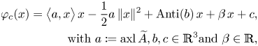 \begin{align*} \varphi_c(x)=\big\langle{a},{x}\big\rangle\,x-\frac 12a\,\lVert{x}\rVert^{2}+\operatorname{Anti}(b)\,x +\beta\,x +c, \\ \text{with }a: = \operatorname{axl}\widetilde A,b,c\in\mathbb{R}^{3} \text{and }\beta\in\mathbb{R}, \end{align*}
namely the infinitesimal conformal mappings, cf. [Reference Dain17, Reference Jeong and Neff33, Reference Neff, Jeong and Ramezani49, Reference Reshetnyak63–Reference Schirra65], see figure 1 for an illustration in 2D.
Figure 1. In the planar case, the condition  $\operatorname {dev}_2\operatorname {sym} \operatorname {D}\hspace {-1pt} u=0$ coincides with the Cauchy-Riemann equations for the function
  $u$ (see appendix). Therefore, infinitesimal conformal mappings in 2D are holomorphic functions which preserve angles exactly. This ceases to be the case for 3D infinitesimal conformal mappings defined by
  $\operatorname {dev}_3\operatorname {sym} \operatorname {D}\hspace {-1pt} u=0$.
A first proof of (1.18), even in all dimensions  $n\geq 3$, was given by Reshetnyak [Reference Reshetnyak63] over domains which are star-like with respect to a ball. Over bounded Lipschitz domains the trace-free Korn's second inequality in all dimensions
  $n\geq 3$, namely
 \begin{align} &\exists c > 0\ \forall\, u\in W^{1,p}(\Omega,\mathbb{R}^{n}):\nonumber\\ &\quad\lVert{u}\rVert_{W^{1,p}(\Omega,\mathbb{R}^{n})}\leq c\, \left(\lVert{u}\rVert_{L^{p}(\Omega,\mathbb{R}^{n})} + \lVert{\operatorname{dev}_n\operatorname{sym}\operatorname{D}\hspace{-1pt} u}\rVert_{L^{p}(\Omega,\mathbb{R}^{n\times n})} \right), \end{align}
was justified by Dain [Reference Dain17] in the case  $p=2$ and by Schirra [Reference Schirra65] for all
  $p>1$. Their proofs use again the Lions lemma and the ‘higher order’ analogues of the differential relation (1.8):
 \begin{equation} \operatorname{D}\hspace{-1pt}\Delta u = L(\operatorname{D}\hspace{-1pt}^{2} \operatorname{dev}_n\operatorname{sym} \operatorname{D}\hspace{-1pt} u).\end{equation}
However, the differential operators  $\operatorname {sym} \operatorname {D}\hspace {-1pt}$ and
  $\operatorname {dev}_n\operatorname {sym} \operatorname {D}\hspace {-1pt}$ are particular cases of the so-called coercive elliptic operators whose study began with Aronszajn [Reference Aronszajn5].
Let us go back to
 \begin{equation} \lVert{ P }\rVert_{L^{2}(\Omega,\mathbb{R}^{3\times 3})}\leq c\,\left(\lVert{\operatorname{dev} \operatorname{sym} P }\rVert_{L^{2}(\Omega,\mathbb{R}^{3\times 3})} + \lVert{ \operatorname{dev} \operatorname{Curl} P }\rVert_{L^{2}(\Omega,\mathbb{R}^{3\times 3})}\right)\end{equation}
whose first proof for  $P\in W^{1,2}_0(\operatorname {Curl}; \Omega ,\mathbb {R}^{3\times 3})$ was given in [Reference Bauer, Neff, Pauly and Starke6] via the trace-free classical Korn's inequality, a Maxwell estimate and a Helmholtz decomposition and is not directly amenable to the
  $L^{p}$-case. Here, we catch up with the latter.
In the following section we start by summarizing the notations and collect some preliminary results from algebraic calculations which are needed in the subsequent vector calculus to establish relations of the type:
 \begin{equation} \operatorname{D}\hspace{-1pt}^{3}(A+\zeta\cdot{\mathbb{1}}) = L (\operatorname{D}\hspace{-1pt}^{2}\operatorname{dev} \operatorname{Curl} (A+\zeta\cdot {\mathbb{1}}))\end{equation}
for skew-symmetric tensor fields  $A$ and scalar functions
  $\zeta$, where
  $L$ denotes a corresponding constant coefficients linear operator. Based on this ‘higher order’ analogue of the differential relation (1.7) we prove our main results in the last section using a similar argumentation as in [Reference Dain17, Reference Schirra65] which argue by the Lions lemma resp. Nečas estimate and the compact embedding
  $W^{1,p}(\Omega )\subset \!\subset L^{p}(\Omega )$.
2. Notations and preliminaries
Let  $n\geq 2$. We consider for vectors
  $a,b\in \mathbb {R}^{n}$ the scalar product
  $\big \langle {a},{b}\big \rangle : = \sum _{i=1}^{n} a_i\,b_i \in \mathbb {R}$, the (squared) norm
  $\lVert {a}\rVert ^{2}: = \big \langle {a},{a}\big \rangle$ and the dyadic product
  $a\otimes b : = (a_i\,b_j)_{i,j=1,\ldots ,n}\in \mathbb {R}^{n\times n}$. Similarly, we define the scalar product for matrices
  $P,Q\in \mathbb {R}^{n\times n}$ by
  $\big \langle {P},{Q}\big \rangle : = \sum _{i,j=1}^{n} P_{ij}\,Q_{ij} \in \mathbb {R}$ and the (squared) Frobenius-norm by
  $\lVert {P}\rVert ^{2}: = \big \langle {P},{P}\big \rangle$. We highlight by
  $.\cdot .$ the scalar multiplication of a scalar with a matrix, whereas matrix multiplication is denoted only by juxtaposition.
Moreover,  $P^{T}: = (P_{ji})_{i,j=1,\ldots ,n}$ denotes the transposition of the matrix
  $P=(P_{ij})_{i,j=1,\ldots ,n}$. The latter decomposes orthogonally into the symmetric part
  $\operatorname {sym} P : = \frac 12(P+P^{T})$ and the skew-symmetric part
  $\operatorname {skew} P : = \frac 12(P-P^{T})$. We will denote by
  $\mathfrak {so}(n): = \{A\in \mathbb {R}^{n\times n}\mid A^{T} = -A\}$ the Lie-Algebra of skew-symmetric matrices.
For the identity matrix we will write  ${\mathbb{1}}$, so that the trace of a squared matrix
  $P$ is given by
  $\operatorname {tr} P : = \big \langle {P},{{\mathbb{1}}}\big \rangle$. The deviatoric (trace-free) part of
  $P$ is given by
  $\operatorname {dev}_n P: = P -\frac 1n\operatorname {tr}(P) {\cdot }{\mathbb{1}}$ and in three dimensions its index will be suppressed, i.e. we write
  $\operatorname {dev}$ instead of
  $\operatorname {dev}_3$.
We will denote by  $\mathscr {D}'(\Omega )$ the space of distributions on a bounded Lipschitz domain
  $\Omega \subset \mathbb {R}^{n}$ and by
  $W^{-k,p}(\Omega )$ the dual space of
  $W^{k,p'}_0(\Omega )$, where
  $p'=\frac {p}{p-1}$ is the Hölder dual exponent to
  $p$.
$p$.
Throughout the paper we use  $c$ as a generic positive constant, which is not necessarily the same in any two places, and we use
  $L(.)$ as a generic linear operator with constant coefficients, which also may differ in any two places within the paper.
In  $3$-dimensions we make use of the vector product
  $\times :\mathbb {R}^{3}\times \mathbb {R}^{3} \to \mathbb {R}^{3}$. Since the vector product
  $a\times .$ with a fixed vector
  $a\in \mathbb {R}^{3}$ is linear in the second component, there exists a unique matrix
  $\operatorname {Anti}(a)$ such that
 \begin{equation} a\times b = : \operatorname{Anti}(a) b \quad \forall\, b\in\mathbb{R}^{3},\end{equation}
and direct calculations show that for  $a=(a_1,a_2,a_3)^{T}$ the matrix
  $\operatorname {Anti}(a)$ has the form
 \begin{equation} \operatorname{Anti}(a)=\begin{pmatrix} 0 & -a_3 & a_2\\ a_3 & 0 & -a_1\\ - a_2 & a_1 & 0\end{pmatrix}. \end{equation}
The inverse of  $\operatorname {Anti}:\mathbb {R}^{3}\to \mathfrak {so}(3)$ is denoted by
  $\operatorname {axl}:\mathfrak {so}(3)\to \mathbb {R}^{3}$ and fulfills
  $\operatorname {axl}(A)\times b = A\,b$ for all skew-symmetric
  $(3\times 3)$-matrices
  $A$ and vectors
  $b\in \mathbb {R}^{3}$. The matrix representation of the cross product allows for a generalization towards a cross product of a matrix
  $P\in \mathbb {R}^{3\times 3}$ and a vector
  $b\in \mathbb {R}^{3}$ via
 \begin{equation} P\times b: = P\,\operatorname{Anti}(b),\end{equation}
so, especially, for  $P={\mathbb{1}}$ it holds
 \begin{equation} {\mathbb{1}}\times b ={\mathbb{1}}\operatorname{Anti}(b)=\operatorname{Anti}(b) \qquad \forall\ b\in\mathbb{R}^{3}. \end{equation}
We repeat the following crucial algebraic identity:
 \begin{equation} (\operatorname{Anti} a)\times b = b \otimes a -\big\langle{b},{a}\big\rangle {\cdot} {\mathbb{1}} \quad \forall\ a,b\in\mathbb{R}^{3}. \end{equation}
Observation 3 For  $P\in \mathbb {R}^{3\times 3}$ and
  $b\in \mathbb {R}^{3}$ we have
 \begin{equation} \operatorname{dev}(P\times b)= 0 \ \Leftrightarrow \ P\times b = 0.\end{equation}
Proof. We decompose  $P$ into its symmetric and skew-symmetric part, i.e.,
 \[ P = S + A = S + \operatorname{Anti}(a), \quad \text{for some }S\in\operatorname{Sym}(3), A\in\mathfrak{so}(3)\text{ and with }a=\operatorname{axl}(A). \]
For a symmetric matrix  $S$ it holds
  $\operatorname {tr}(S\times b)= 0$ for any
  $b\in \mathbb {R}^{3}$, sinceFootnote 2
 \begin{equation} \operatorname{tr}(S\times b)=\big\langle{S\times b},{{\mathbb{1}}}\big\rangle_{\mathbb{R}^{3\times 3}}=\big\langle{S\operatorname{Anti}(b)},{{\mathbb{1}}}\big\rangle_{\mathbb{R}^{3\times 3}} ={-}\big\langle{S},{\operatorname{Anti}(b)}\big\rangle_{\mathbb{R}^{3\times 3}}\overset{S\in\operatorname{Sym}(3)}{=}0. \end{equation}
Thus, using the decomposition  $P = S + \operatorname {Anti}(a)$, we have:
 \begin{align} \operatorname{dev}(P\times b) &= P\times b -\frac 13\operatorname{tr}(P\times b) {\cdot}{\mathbb{1}} \overset{(2.7)}{=} P\times b -\frac 13\operatorname{tr}((\operatorname{Anti} a)\times b) {\cdot}{\mathbb{1}}\nonumber\\ &\overset{(2.5)}{=}\ P\times b - \frac 13\operatorname{tr}(b\otimes a -\big\langle{b},{a}\big\rangle {\cdot}{\mathbb{1}}) {\cdot}{\mathbb{1}} = P\times b +\frac 23\big\langle{a},{b}\big\rangle {\cdot}{\mathbb{1}}. \end{align}
Moreover, for any matrix  $P\in \mathbb {R}^{3\times 3}$ we note that
 \begin{equation} (P\times b)\,b = (P\operatorname{Anti}(b)) b = P(\operatorname{Anti}(b)\, b)=P(b\times b) =0. \end{equation}
Thus, we obtain
 \begin{equation}
\left\langle{b},{\operatorname{dev}(P\times
b)\,b}\right\rangle
\overset{(2.8)}{=}\left\langle{b},{\left(P\times b +\frac
23\big\langle{a},{b}\big\rangle {\cdot}{\mathbb{1}}\right)\,
b}\right\rangle \overset{(2.9)}{=} \frac
23\big\langle{a},{b}\big\rangle\,\lVert{b}\rVert^{2},
\end{equation}
\begin{equation}
\left\langle{b},{\operatorname{dev}(P\times
b)\,b}\right\rangle
\overset{(2.8)}{=}\left\langle{b},{\left(P\times b +\frac
23\big\langle{a},{b}\big\rangle {\cdot}{\mathbb{1}}\right)\,
b}\right\rangle \overset{(2.9)}{=} \frac
23\big\langle{a},{b}\big\rangle\,\lVert{b}\rVert^{2},
\end{equation}and the conclusion follows from the identity
 \begin{align} \lVert{b}\rVert^{2} {\cdot} P\times b &\overset{(2.8)}{=} \lVert{b}\rVert^{2} {\cdot} \operatorname{dev}(P\times b)-\frac 23\lVert{b}\rVert^{2}\big\langle{a},{b}\big\rangle {\cdot}{\mathbb{1}}\nonumber\\ &\overset{(2.10)}{=} \lVert{b}\rVert^{2} {\cdot} \operatorname{dev}(P\times b) - \big\langle{b},{\operatorname{dev}(P\times b)\,b}\big\rangle {\cdot}{\mathbb{1}}. \end{align}
An application of the Cauchy-Bunyakovsky-Schwarz inequality on the right-hand side of (2.11) shows that
 \begin{equation} \lVert{\operatorname{dev}(P\times b)}\rVert \le \lVert{P\times b}\rVert \le \left(1+\sqrt{3}\right)\lVert{\operatorname{dev}(P\times b)}\rVert.\end{equation}
Observation 4 Let  $a\in \mathbb {R}^{3}$ and
  $\alpha \in \mathbb {R}$, then
 \[ (\operatorname{Anti}(a)+\alpha\cdot{\mathbb{1}})\times b= 0 \text{ for } b\in\mathbb{R}^{3}\backslash\{0\} \quad \Rightarrow \quad a=0 \text{ and } \alpha=0. \]
Proof. By (2.5) and (2.4) we have:
 \begin{equation} 0 = (\operatorname{Anti}(a)+\alpha\cdot{\mathbb{1}})\times b = b\otimes a -\big\langle{b},{a}\big\rangle {\cdot}{\mathbb{1}} + \alpha\cdot \operatorname{Anti}(b). \end{equation}
Taking the trace on both sides we obtain
 \[ 0 = \operatorname{tr}( b\otimes a -\big\langle{b},{a}\big\rangle {\cdot}{\mathbb{1}} + \alpha\cdot \operatorname{Anti}(b)) = \big\langle{a},{b}\big\rangle-3\,\big\langle{a},{b}\big\rangle ={-}2\,\big\langle{a},{b}\big\rangle. \]
Thus, reinserting  $\big \langle {b},{a}\big \rangle =0$ in (2.13) and applying
  $\operatorname {sym}$ on both sides, this implies
  $\operatorname {sym}(b\otimes a)=0$. Since
 \begin{equation} \lVert{\operatorname{sym}(a\otimes b)}\rVert^{2} = \frac 12\lVert{a}\rVert^{2}\lVert{b}\rVert^{2}+\frac 12\big\langle{a},{b}\big\rangle^{2}\end{equation}
and  $b\neq 0$ we must have
  $a=0$. Hence, by (2.13) also
  $\alpha =0$.
Formally the gradient and the curl of a vector field  $a:\Omega \to \mathbb {R}^{3}$ can be seen as
 \[ \operatorname{D}\hspace{-1pt} a = a\otimes \nabla \quad \text{and}\quad \operatorname{curl} a = a\times (-\nabla). \]
The latter also generalizes to  $(3\times 3)$-matrix fields
  $P:\Omega \to \mathbb {R}^{3\times 3}$ row-wise:Footnote 3
 \begin{equation} \operatorname{Curl} P = P \times (-\nabla) = \begin{pmatrix} (P^{T} e_1)^{T} \\ (P^{T}e_2)^{T} \\ (P^{T}e_3)^{T} \end{pmatrix} \times (-\nabla) =\begin{pmatrix} (\operatorname{curl}\,(P^{T}e_1))^{T} \\ (\operatorname{curl}\,(P^{T}e_2))^{T} \\ (\operatorname{curl}\,(P^{T}e_3))^{T} \end{pmatrix}\in\mathbb{R}^{3\times 3}. \end{equation}
Replacing  $b$ by
  $\nabla$ in (2.5) we obtain Nye's formulas
 \begin{equation} \operatorname{Curl} A = \operatorname{tr}(\operatorname{D}\hspace{-1pt} \operatorname{axl} A)\cdot{\mathbb{1}}- (\operatorname{D}\hspace{-1pt} \operatorname{axl} A)^{T},\end{equation}
and
 \begin{equation} \operatorname{D}\hspace{-1pt} \operatorname{axl} A = \frac 12 \,\operatorname{tr}(\operatorname{Curl} A)\cdot{\mathbb{1}} - (\operatorname{Curl} A)^{T}\end{equation}
for all skew-symmetric  $(3\times 3)$-matrix fields
  $A$.
$A$.
Remark 5 Formal calculations (e.g. replacing  $b$ by
  $\nabla$) have to be performed very carefully. Indeed, they are allowed in algebraic identities but fail, in general, for implications, e.g. for
  $A\in \mathfrak {so}(3)$ and
  $b\in \mathbb {R}^{3}$ we have
  $A\times b = 0$ if and only if
  $\operatorname {dev}(A\times b)= 0$, since the following expression holds true, cf. Observation 3 and (2.11):
 \begin{equation} \lVert{b}\rVert^{2} {\cdot} A\times b =\lVert{b}\rVert^{2} {\cdot} \operatorname{dev}(A\times b) - \big\langle{b},{\operatorname{dev}(A\times b)\,b}\big\rangle {\cdot}{\mathbb{1}}\,. \end{equation}
However,  $\operatorname {dev}(\operatorname {Curl} A)=\operatorname {dev}(A\times (-\nabla ))=0$ does not imply already that
  $\operatorname {Curl} A = A\times (-\nabla )= 0$, due to the counterexample
  $A=\operatorname {Anti}(x)$, since by Nye's formula (2.16) we have
  $\operatorname {Curl}(\operatorname {Anti}(x))=2\cdot {\mathbb{1}}$. Of course, we can interpret (2.17) also in the sense of vector calculus, which gives then an expression for
  $\Delta \operatorname {Curl} A$ in terms of the second distributional derivatives of
  $\operatorname {dev}(\operatorname {Curl} A)$, but, the latter would have no meaning for the relation of
  $\operatorname {Curl} A$ and
  $\operatorname {dev}\operatorname {Curl} A$.
Lemma 6 Let  $A\in \mathscr {D}'(\Omega ,\mathfrak {so}(3))$ and
  $\zeta \in \mathscr {D}'(\Omega ,\mathbb {R})$. Then
(a) the entries of
 $\operatorname {D}\hspace {-1pt}^{2} (A+\zeta \cdot {\mathbb{1}})$ are linear combinations of the entries of $\operatorname {D}\hspace {-1pt}\operatorname {Curl} (A+\zeta \cdot {\mathbb{1}})$.
(b) the entries of
$\operatorname {D}\hspace {-1pt}^{2} A$ are linear combinations of the entries of $\operatorname {D}\hspace {-1pt}\operatorname {dev}\operatorname {Curl} A$.(c) the entries of
$\operatorname {D}\hspace {-1pt}^{3} (A+\zeta \cdot {\mathbb{1}})$ are linear combinations of the entries of $\operatorname {D}\hspace {-1pt}^{2} \operatorname {dev}\operatorname {Curl}(A+\zeta \cdot {\mathbb{1}})$.


Proof. Observe that applying (2.4) to the vector field  $\nabla \zeta$ we obtain:
 \begin{equation} \operatorname{Curl} (\zeta\cdot{\mathbb{1}}) \overset{(2.15)}{=} {\mathbb{1}} \times (-\nabla \zeta) \overset{(2.4)}{=} -\operatorname{Anti}(\nabla \zeta). \end{equation}
Let us first start by proving part (b). From Nye's formula (2.16a) we obtain
 \begin{equation} \operatorname{dev} \operatorname{Curl} A = \frac 13\operatorname{tr}(\operatorname{D}\hspace{-1pt}\operatorname{axl} A) {\cdot}{\mathbb{1}} - (\operatorname{D}\hspace{-1pt}\operatorname{axl} A)^{T}\end{equation}
so that taking the  $\operatorname {Curl}$ of the transpositions on both sides gives
 \begin{equation} \operatorname{Curl}([ \operatorname{dev} \operatorname{Curl} A]^{T}) \underset{(2.19)}{\overset{\operatorname{Curl} \circ \operatorname{D}\hspace{-1pt}\, \equiv 0}{=} } \frac 13\operatorname{Curl}(\operatorname{tr}(\operatorname{D}\hspace{-1pt}\operatorname{axl} A) {\cdot}{\mathbb{1}}) \overset{(2.18)}{=} - \frac 13\operatorname{Anti}(\nabla \operatorname{tr}(\operatorname{D}\hspace{-1pt}\operatorname{axl} A)). \end{equation}
In other words, we have that 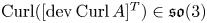 $\operatorname {Curl}([ \operatorname {dev} \operatorname {Curl} A]^{T})\in \mathfrak {so}(3)$, and applying
  $\operatorname {axl}$ on both sides of (2.20) we obtain
 \begin{equation} \nabla \operatorname{tr}(\operatorname{D}\hspace{-1pt}\operatorname{axl} A) ={-}3\operatorname{axl}(\operatorname{Curl}([ \operatorname{dev} \operatorname{Curl} A]^{T})) = L_0(\operatorname{D}\hspace{-1pt}\operatorname{dev} \operatorname{Curl} A). \end{equation}
Taking the  $\partial _j$-derivative of (2.19) for
  $j=1,2,3$ we conclude
 \begin{equation} \partial_j(\operatorname{D}\hspace{-1pt}\operatorname{axl} A)^{T} \overset{(2.19)}{=} \frac 13\partial_j\operatorname{tr}(\operatorname{D}\hspace{-1pt}\operatorname{axl} A)-\partial_j\operatorname{dev} \operatorname{Curl} A \overset{(2.21)}{=}\widetilde L_0(\operatorname{D}\hspace{-1pt}\operatorname{dev} \operatorname{Curl} A)\,, \end{equation}
which establishes part (b), namely 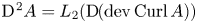 $\operatorname {D}\hspace {-1pt}^{2} A = L_2(\operatorname {D}\hspace {-1pt}(\operatorname {dev} \operatorname {Curl} A))$ for skew-symmetric tensor fields
  $A$.
$A$.
The proof of part (a) is divided into the following two key observations:
 \[\hbox{(a.i) }\operatorname {D}^{2} \zeta = \widetilde L_1(\operatorname {D}\operatorname {Curl} (A+\zeta \cdot {\mathbb{1}})),\quad \hbox{(a.ii) }\operatorname {D}^{2} A = \widetilde L_2(\operatorname {D}\operatorname {Curl} (A+\zeta \cdot {\mathbb{1}})). \]
To show that each entry of the Hessian matrix  $\operatorname {D}\hspace {-1pt}^{2} \zeta$ is a linear combination of the entries of
  $\operatorname {D}\hspace {-1pt}\operatorname {Curl} (A+\zeta \cdot {\mathbb{1}})$ we make use of the second-order differential operator
  $\boldsymbol {\operatorname {inc}}\,$ given for
  $B\in \mathscr {D}'(\Omega ,\mathbb {R}^{3\times 3})$ viaFootnote 4
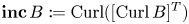 \begin{equation} \boldsymbol{\operatorname{inc}}\, B : = \operatorname{Curl} ([\operatorname{Curl} B]^{T})\end{equation}
so that
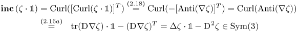 \begin{align} \boldsymbol{\operatorname{inc}}\, (\zeta\cdot{\mathbb{1}}) &= \operatorname{Curl} ([\operatorname{Curl}(\zeta\cdot{\mathbb{1}})]^{T})\overset{(2.18)}{=}\operatorname{Curl} (-[\operatorname{Anti}(\nabla \zeta)]^{T}) = \operatorname{Curl} (\operatorname{Anti}(\nabla \zeta))\nonumber\\ &\overset{(2.16a)}{=}\ \ \operatorname{tr}(\operatorname{D}\hspace{-1pt}\nabla\zeta)\cdot{\mathbb{1}}-(\operatorname{D}\hspace{-1pt}\nabla \zeta)^{T} = \Delta \zeta\cdot {\mathbb{1}} - \operatorname{D}\hspace{-1pt}^{2} \zeta \in \operatorname{Sym}(3) \end{align}
is symmetric. On the other hand, for a skew-symmetric matrix field 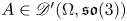 $A\in \mathscr {D}'(\Omega ,\mathfrak {so}(3))$ we have that
 \begin{align} \boldsymbol{\operatorname{inc}}\, A &= \operatorname{Curl} ([\operatorname{Curl} A]^{T}) \overset{(2.16)}{=} \operatorname{Curl} ( \operatorname{tr} (\operatorname{D}\hspace{-1pt} \operatorname{axl} A)\cdot {\mathbb{1}} - \operatorname{D}\hspace{-1pt} \operatorname{axl} A )\nonumber\\ &\overset{\operatorname{Curl} \circ \operatorname{D}\hspace{-1pt}\, \equiv 0}{=}\ \operatorname{Curl} ( \operatorname{tr} (\operatorname{D}\hspace{-1pt} \operatorname{axl} A)\cdot {\mathbb{1}}) \overset{(2.18)}{=}-\operatorname{Anti} (\nabla\operatorname{tr} (\operatorname{D}\hspace{-1pt} \operatorname{axl} A))\in\mathfrak{so}(3) \end{align}
is skew-symmetric. Hence,
 \begin{equation} \operatorname{sym} (\boldsymbol{\operatorname{inc}}\, (A+\zeta\cdot{\mathbb{1}})) = \Delta \zeta\cdot {\mathbb{1}} - \operatorname{D}\hspace{-1pt}^{2} \zeta \quad \text{and}\quad \operatorname{tr} (\boldsymbol{\operatorname{inc}}\, (A+\zeta\cdot{\mathbb{1}})) = 2\,\Delta\zeta . \end{equation}
In other words, the entries of the Hessian matrix of  $\zeta$ are linear combinations of entries from
 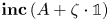 $\boldsymbol {\operatorname {inc}}\, (A+\zeta \cdot {\mathbb{1}})$:
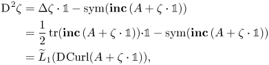 \begin{align}
\operatorname{D}\hspace{-1pt}^{2}\zeta &= \Delta \zeta\cdot
{\mathbb{1}} - \operatorname{sym}
(\boldsymbol{\operatorname{inc}}\,
(A+\zeta\cdot{\mathbb{1}}))\notag\\
& = \frac
12\operatorname{tr} (\boldsymbol{\operatorname{inc}}\,
(A+\zeta\cdot{\mathbb{1}}))
{\cdot{\mathbb{1}}} -
\operatorname{sym} (\boldsymbol{\operatorname{inc}}\,
(A+\zeta\cdot{\mathbb{1}}))\nonumber\\
&= \widetilde
L_1(\operatorname{D}\hspace{-1pt}\operatorname{Curl}
(A+\zeta\cdot{\mathbb{1}})),
\end{align}
\begin{align}
\operatorname{D}\hspace{-1pt}^{2}\zeta &= \Delta \zeta\cdot
{\mathbb{1}} - \operatorname{sym}
(\boldsymbol{\operatorname{inc}}\,
(A+\zeta\cdot{\mathbb{1}}))\notag\\
& = \frac
12\operatorname{tr} (\boldsymbol{\operatorname{inc}}\,
(A+\zeta\cdot{\mathbb{1}}))
{\cdot{\mathbb{1}}} -
\operatorname{sym} (\boldsymbol{\operatorname{inc}}\,
(A+\zeta\cdot{\mathbb{1}}))\nonumber\\
&= \widetilde
L_1(\operatorname{D}\hspace{-1pt}\operatorname{Curl}
(A+\zeta\cdot{\mathbb{1}})),
\end{align}
where we have used that the entries of  $\boldsymbol {\operatorname {inc}}\, B$ are, of course, linear combinations of entries of
  $\operatorname {D}\hspace {-1pt} \operatorname {Curl} B$.
To establish (a.ii) from (a.i), recall that for a skew-symmetric matrix field  $A$ the entries of
  $\operatorname {D}\hspace {-1pt} A$ are linear combinations of the entries from
  $\operatorname {Curl} A$:
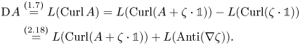 \begin{align} \operatorname{D}\hspace{-1pt} A &\overset{(1.7)}{=} L (\operatorname{Curl} A) = L(\operatorname{Curl}(A+\zeta\cdot{\mathbb{1}}))- L(\operatorname{Curl} (\zeta\cdot {\mathbb{1}})) \nonumber\\ &\overset{(2.18)}{=} L(\operatorname{Curl}(A+\zeta\cdot{\mathbb{1}})) + L(\operatorname{Anti} (\nabla \zeta)). \end{align}
We conclude by taking the  $\partial _j$-derivative of (2.28) for
  $j=1,2,3$, namely
 \[ \partial_j \operatorname{D}\hspace{-1pt} A = L(\partial_j\operatorname{Curl}(A+\zeta\cdot{\mathbb{1}})) + L(\partial_j\operatorname{Anti} (\nabla \zeta)) \overset{({\rm a,i})}{=} \widetilde L_3(\operatorname{D}\hspace{-1pt}\operatorname{Curl}(A+\zeta\cdot{\mathbb{1}})). \]
Finally, we establish part (c) arguing in a similar way by showing the following linear combinations:
(1)
$\operatorname {D}\hspace {-1pt}^{2} \zeta = \widetilde L_4(\operatorname {D}\hspace {-1pt}\operatorname {dev}\operatorname {Curl} (A+\zeta \cdot {\mathbb{1}}))$,(2)
$\operatorname {D}\hspace {-1pt}^{3} A =\widetilde L_7(\operatorname {D}\hspace {-1pt}^{2}\operatorname {dev}\operatorname {Curl} (A+\zeta \cdot {\mathbb{1}}))$.

Regarding (2.18) and (2.16) we have
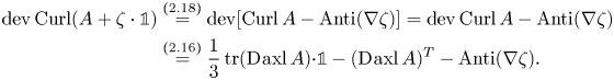 \begin{align} \operatorname{dev}\operatorname{Curl}(A+\zeta\cdot{\mathbb{1}}) &\overset{(2.18)}{=} \operatorname{dev}[\operatorname{Curl} A -\operatorname{Anti}(\nabla \zeta)] =\operatorname{dev}\operatorname{Curl} A -\operatorname{Anti}(\nabla \zeta)\nonumber\\ &\overset{(2.16)}{=} \frac 13\operatorname{tr}(\operatorname{D}\hspace{-1pt}\operatorname{axl} A) {\cdot}{\mathbb{1}}-(\operatorname{D}\hspace{-1pt}\operatorname{axl} A)^{T} -\operatorname{Anti}(\nabla \zeta). \end{align}
 Transposing and taking the  $\operatorname {Curl}$ on both sides yields
 \begin{align} \operatorname{Curl} ([\operatorname{dev}\operatorname{Curl}(A+\zeta\cdot{\mathbb{1}})]^{T}) \underset{\operatorname{Curl} \circ \operatorname{D}\hspace{-1pt}\, \equiv 0}{\overset{(2.18), (2.16)}{=}} -\frac 13\underset{\in\mathfrak{so}(3)}{\underbrace{\operatorname{Anti}(\nabla \operatorname{tr}(\operatorname{D}\hspace{-1pt}\operatorname{axl} A))}}+ \underset{\in\operatorname{Sym}(3)}{\underbrace{\Delta \zeta\cdot {\mathbb{1}} - \operatorname{D}\hspace{-1pt}^{2}\zeta}} \end{align}
and we obtain, similar to the decomposition in (2.27):
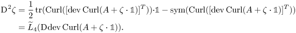 \begin{align} \operatorname{D}\hspace{-1pt}^{2}\zeta &= \frac 12\operatorname{tr}(\operatorname{Curl} ([\operatorname{dev}\operatorname{Curl}(A+\zeta\cdot{\mathbb{1}})]^{T}) ) {\cdot{\mathbb{1}}}- \operatorname{sym}(\operatorname{Curl} ([\operatorname{dev}\operatorname{Curl}(A+\zeta\cdot{\mathbb{1}})]^{T}) )\nonumber\\ & = \widetilde L_4(\operatorname{D}\hspace{-1pt}\operatorname{dev}\operatorname{Curl}(A+\zeta\cdot{\mathbb{1}})). \end{align}
On the other hand, taking  $\boldsymbol {\operatorname {inc}}\,$ of the transpositions on both sides of (2.29) gives
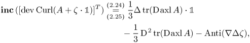 \begin{align}
\boldsymbol{\operatorname{inc}}\,([\operatorname{dev}\operatorname{Curl}(A+\zeta\cdot{\mathbb{1}})]^{T}) &\underset{(2.25)}{\overset{(2.24)}{=}}
\frac 13\Delta
\operatorname{tr}(\operatorname{D}\hspace{-1pt}\operatorname{axl}
A)\cdot{\mathbb{1}}\notag\\
&\qquad - \frac 13
\operatorname{D}\hspace{-1pt}^{2}\operatorname{tr}(\operatorname{D}\hspace{-1pt}\operatorname{axl}
A)-\operatorname{Anti}(\nabla \Delta \zeta),
\end{align}
\begin{align}
\boldsymbol{\operatorname{inc}}\,([\operatorname{dev}\operatorname{Curl}(A+\zeta\cdot{\mathbb{1}})]^{T}) &\underset{(2.25)}{\overset{(2.24)}{=}}
\frac 13\Delta
\operatorname{tr}(\operatorname{D}\hspace{-1pt}\operatorname{axl}
A)\cdot{\mathbb{1}}\notag\\
&\qquad - \frac 13
\operatorname{D}\hspace{-1pt}^{2}\operatorname{tr}(\operatorname{D}\hspace{-1pt}\operatorname{axl}
A)-\operatorname{Anti}(\nabla \Delta \zeta),
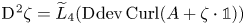
\end{align}yielding the relation
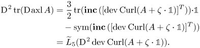 \begin{align} \operatorname{D}\hspace{-1pt}^{2} \operatorname{tr}(\operatorname{D}\hspace{-1pt}\operatorname{axl} A) &= \frac 32\operatorname{tr}(\boldsymbol{\operatorname{inc}}\,([\operatorname{dev}\operatorname{Curl}(A+\zeta\cdot{\mathbb{1}})]^{T})) {\cdot{\mathbb{1}}}\nonumber\\ &\quad-\operatorname{sym}(\boldsymbol{\operatorname{inc}}\,([\operatorname{dev}\operatorname{Curl}(A+\zeta\cdot{\mathbb{1}})]^{T})) \nonumber\\ &=\widetilde L_5(\operatorname{D}\hspace{-1pt}^{2} \operatorname{dev}\operatorname{Curl}(A+\zeta\cdot{\mathbb{1}})). \end{align}
Considering the second distributional derivatives in (2.29) we conclude
 \begin{align*} \operatorname{D}\hspace{-1pt}^{3} \operatorname{axl} A &= \frac 13 \operatorname{D}\hspace{-1pt}^{2} \operatorname{tr}(\operatorname{D}\hspace{-1pt}\operatorname{axl} A) {\cdot} {\mathbb{1}} -\operatorname{D}\hspace{-1pt}^{2}([\operatorname{dev}\operatorname{Curl}(A+\zeta\cdot{\mathbb{1}})]^{T})+\operatorname{D}\hspace{-1pt}^{2}\operatorname{Anti}(\nabla \zeta)\\ &\underset{(2.33)}{\overset{(2.31)}{=}}\widetilde L_6(\operatorname{D}\hspace{-1pt}^{2} \operatorname{dev}\operatorname{Curl}(A+\zeta\cdot{\mathbb{1}})).\end{align*}
□
Remark 7 In the above proof we have used that the second-order differential operator  $\boldsymbol {\operatorname {inc}}\,$ does not change the symmetry property after application on square matrix fields, cf. the appendix. Further properties are collected e.g. in [Reference Neff, Ghiba, Madeo, Placidi and Rosi52, appendix], [Reference Amrouche, Ciarlet, Gratie and Kesavan1, sec. 2] and [Reference Ciarlet12, sec. 6.18].
The incompatibility operator  $\boldsymbol {\operatorname {inc}}\,$ arises in dislocation models, e.g., in the modelling of elastic materials with dislocations or in the modelling of dislocated crystals, since the strain cannot be a symmetric gradient of a vector field as soon as dislocations are present and the notion of incompatibility is at the basis of a new paradigm to describe the inelastic effects, cf. [Reference Amstutz and Van Goethem3, Reference Amstutz and Van Goethem4, Reference Ebobisse and Neff20, Reference Maggiani, Scala and Van Goethem46], cf. the appendix for further comments.
Moreover, the equation  $\boldsymbol {\operatorname {inc}}\,\operatorname {sym} e\equiv 0$ is equivalent to the Saint-Venant compatibility condition Footnote 5 defining the relation between the symmetric strain
  $\operatorname {sym} e$ and the displacement vector field
  $u$:
$u$:
 \begin{equation} \boldsymbol{\operatorname{inc}}\, \operatorname{sym} e \equiv 0 \quad \Leftrightarrow \quad \operatorname{sym} e = \operatorname{sym} \operatorname{D}\hspace{-1pt} u \end{equation}
over simply connected domains, cf. [Reference Amrouche, Ciarlet, Gratie and Kesavan1, Reference Maggiani, Scala and Van Goethem46]. In the appendix we show that the operators  $\boldsymbol {\operatorname {inc}}\,$ and
  $\operatorname {sym}$ can be interchanged, so that
 \begin{equation} \boldsymbol{\operatorname{inc}}\, \operatorname{sym} e = \operatorname{sym} \boldsymbol{\operatorname{inc}}\, e = \operatorname{sym} \operatorname{Curl} ([\operatorname{Curl} e]^{T}).\end{equation}
Investigations over multiply connected domains can be found e.g. in [Reference Geymonat and Krasucki30, Reference Ting66].
Returning to our proof, a crucial ingredient in our following argumentation is
Theorem 8 (Lions lemma and Nečas estimate)
Let  $\Omega \subset \mathbb {R}^{n}$ be a bounded Lipschitz domain. Let
  $m \in \mathbb {Z}$ and
  $p \in (1, \infty )$. Then
  $f \in \mathscr {D}'(\Omega ,\mathbb {R}^{d})$ and
  $\operatorname {D}\hspace {-1pt} f \in W^{m-1,p}(\Omega ,\mathbb {R}^{d\times n})$ imply
  $f \in W^{m,p}(\Omega ,\mathbb {R}^{d})$. Moreover,
 \begin{equation} \lVert{ f}\rVert_{W^{m,\ p}(\Omega,\mathbb{R}^{d})} \le c\ \left(\lVert{ f}\rVert_{W^{m-1,p}(\Omega,\mathbb{R}^{d})} + \lVert{ \operatorname{D}\hspace{-1pt} f }\rVert_{W^{m-1,p}(\Omega,\mathbb{R}^{d\times n})}\right), \end{equation}
with a constant  $c=c(m,p,n,d,\Omega )>0$.
For the proof we refer to [Reference Amrouche and Girault2, proposition 2.10 and theorem 2.3], [Reference Borchers and Sohr7]. However, since we are dealing with higher order derivatives we also need a ‘higher order’ version of the Lions lemma resp. Nečas estimate.
Corollary 9 Let  $\Omega \subset \mathbb {R}^{n}$ be a bounded Lipschitz domain,
  $m \in \mathbb {Z}$ and
  $p \in (1, \infty )$. Denote by
  $\operatorname {D}\hspace {-1pt}^{k} f$ the collection of all distributional derivatives of order
  $k$. Then
  $f \in \mathscr {D}'(\Omega ,\mathbb {R}^{d})$ and
  $\operatorname {D}\hspace {-1pt}^{k} f \in W^{m-k,p}(\Omega ,\mathbb {R}^{d\times n^{k}})$ imply
  $f \in W^{m,p}(\Omega ,\mathbb {R}^{d})$. Moreover,
 \begin{equation} \lVert{ f}\rVert_{W^{m,p}(\Omega,\mathbb{R}^{d})} \le c\,\left(\lVert{ f}\rVert_{W^{m-1,p}(\Omega,\mathbb{R}^{d})} + \lVert{ \operatorname{D}\hspace{-1pt}^{k} f }\rVert_{W^{m-k,p}(\Omega,\mathbb{R}^{d\times n^{k}})}\right), \end{equation}
with a constant  $c=c(m,p,n,d,\Omega )>0$.
Proof. The assertion  $f \in W^{m,p}(\Omega ,\mathbb {R}^{d})$ and the estimate (2.37) follow by inductive application of theorem 8 to
  $\operatorname {D}\hspace {-1pt}^{l} f$ with
  $l=k-1,k-2,\ldots ,0$. Indeed, starting by applying theorem 8 to
  $\operatorname {D}\hspace {-1pt}^{k-1} f$ gives
 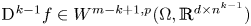 $\operatorname {D}\hspace {-1pt}^{k-1} f \in W^{m-k+1,p}(\Omega ,\mathbb {R}^{d\times n^{k-1}})$ as well as
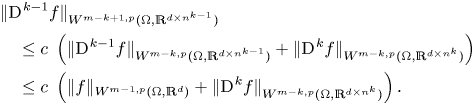 \begin{align} &\lVert{
\operatorname{D}\hspace{-1pt}^{k-1}
f}\rVert_{W^{m-k+1,p}(\Omega,\mathbb{R}^{d\times
n^{k-1}})} \nonumber\\ &\quad \le c\
\left(\lVert{\operatorname{D}\hspace{-1pt}^{k-1}
f}\rVert_{W^{m-k,p}(\Omega,\mathbb{R}^{d\times n^{k-1}})}
+ \lVert{ \operatorname{D}\hspace{-1pt}^{k} f
}\rVert_{W^{m-k,p}(\Omega,\mathbb{R}^{d\times
n^{k}})}\right)\nonumber\\ &\quad \le c\
\left(\lVert{f}\rVert_{W^{m-1,p}(\Omega,\mathbb{R}^{d})}
+ \lVert{ \operatorname{D}\hspace{-1pt}^{k} f
}\rVert_{W^{m-k,p}(\Omega,\mathbb{R}^{d\times
n^{k}})}\right).
\end{align}
\begin{align} &\lVert{
\operatorname{D}\hspace{-1pt}^{k-1}
f}\rVert_{W^{m-k+1,p}(\Omega,\mathbb{R}^{d\times
n^{k-1}})} \nonumber\\ &\quad \le c\
\left(\lVert{\operatorname{D}\hspace{-1pt}^{k-1}
f}\rVert_{W^{m-k,p}(\Omega,\mathbb{R}^{d\times n^{k-1}})}
+ \lVert{ \operatorname{D}\hspace{-1pt}^{k} f
}\rVert_{W^{m-k,p}(\Omega,\mathbb{R}^{d\times
n^{k}})}\right)\nonumber\\ &\quad \le c\
\left(\lVert{f}\rVert_{W^{m-1,p}(\Omega,\mathbb{R}^{d})}
+ \lVert{ \operatorname{D}\hspace{-1pt}^{k} f
}\rVert_{W^{m-k,p}(\Omega,\mathbb{R}^{d\times
n^{k}})}\right).
\end{align}
Now, we can apply theorem 8 to  $\operatorname {D}\hspace {-1pt}^{k-2} f$ to deduce
 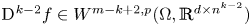 $\operatorname {D}\hspace {-1pt}^{k-2} f \in W^{m-k+2,p}(\Omega ,\mathbb {R}^{d\times n^{k-2}})$ and moreover
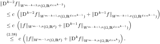 \begin{align} &\lVert{
\operatorname{D}\hspace{-1pt}^{k-2}
f}\rVert_{W^{m-k+2,p}(\Omega,\mathbb{R}^{d\times
n^{k-2}})}\nonumber\\ &\quad \le c\
\left(\lVert{\operatorname{D}\hspace{-1pt}^{k-2}
f}\rVert_{W^{m-k+1,p}(\Omega,\mathbb{R}^{d\times
n^{k-1}})} + \lVert{ \operatorname{D}\hspace{-1pt}^{k-1} f
}\rVert_{W^{m-k+1,p}(\Omega,\mathbb{R}^{d\times
n^{k-1}})}\right)\nonumber\\ &\quad \le c\
\left(\lVert{f}\rVert_{W^{m-1,p}(\Omega,\mathbb{R}^{d})}
+ \lVert{ \operatorname{D}\hspace{-1pt}^{k-1} f
}\rVert_{W^{m-k+1,p}(\Omega,\mathbb{R}^{d\times
n^{k-1}})}\right)\nonumber\\
&\quad \overset{(2.38)}{\le}c\,\left(\lVert{f}\rVert_{W^{m-1,p}(\Omega,\mathbb{R}^{d})}
+ \lVert{ \operatorname{D}\hspace{-1pt}^{k} f
}\rVert_{W^{m-k,p}(\Omega,\mathbb{R}^{d\times
n^{k}})}\right).
\end{align}
\begin{align} &\lVert{
\operatorname{D}\hspace{-1pt}^{k-2}
f}\rVert_{W^{m-k+2,p}(\Omega,\mathbb{R}^{d\times
n^{k-2}})}\nonumber\\ &\quad \le c\
\left(\lVert{\operatorname{D}\hspace{-1pt}^{k-2}
f}\rVert_{W^{m-k+1,p}(\Omega,\mathbb{R}^{d\times
n^{k-1}})} + \lVert{ \operatorname{D}\hspace{-1pt}^{k-1} f
}\rVert_{W^{m-k+1,p}(\Omega,\mathbb{R}^{d\times
n^{k-1}})}\right)\nonumber\\ &\quad \le c\
\left(\lVert{f}\rVert_{W^{m-1,p}(\Omega,\mathbb{R}^{d})}
+ \lVert{ \operatorname{D}\hspace{-1pt}^{k-1} f
}\rVert_{W^{m-k+1,p}(\Omega,\mathbb{R}^{d\times
n^{k-1}})}\right)\nonumber\\
&\quad \overset{(2.38)}{\le}c\,\left(\lVert{f}\rVert_{W^{m-1,p}(\Omega,\mathbb{R}^{d})}
+ \lVert{ \operatorname{D}\hspace{-1pt}^{k} f
}\rVert_{W^{m-k,p}(\Omega,\mathbb{R}^{d\times
n^{k}})}\right).
\end{align}
Consequently, for all  $l=k-1,k-2,\ldots ,0$ we deduce
  $\operatorname {D}\hspace {-1pt}^{l} f \in W^{m-l,p}(\Omega ,\mathbb {R}^{d\times n^{l}})$ as well as
 \begin{equation} \lVert{ \operatorname{D}\hspace{-1pt}^{l} f}\rVert_{W^{m-l,p}(\Omega,\mathbb{R}^{d\times n^{l}})} \le c\,\left(\lVert{f}\rVert_{W^{m-1,p}(\Omega,\mathbb{R}^{d})} + \lVert{ \operatorname{D}\hspace{-1pt}^{k} f }\rVert_{W^{m-k,p}(\Omega,\mathbb{R}^{d\times n^{k}})}\right). \end{equation}
Remark 10 The need to consider higher order derivatives is indicated by the appearance of linear terms in the kernel of Korn's quantitative versions, similar to the situation at the classical trace-free Korn inequalities [Reference Dain17, Reference Schirra65]. In our case we have:
Lemma 11 Let  $A\in L^{p}(\Omega ,\mathfrak {so}(3))$ and
  $\zeta \in L^{p}(\Omega ,\mathbb {R})$. Then we have in the distributional sense
(a)
$\operatorname {Curl}(A+\zeta \cdot {\mathbb{1}})\equiv 0$ if and only if $A+\zeta \cdot {\mathbb{1}}=\operatorname {Anti}(\widetilde {A}\,x+b) +(\big \langle {\operatorname {axl} \widetilde {A}},{x}\big \rangle +\beta )\cdot {\mathbb{1}}$ a.e. on $\Omega ,$(b)
$\operatorname {dev}\operatorname {Curl} A \equiv 0$ if and only if $A= \operatorname {Anti}(\beta \,x+b)$ a.e. on $\Omega ,$(c)
$\operatorname {dev}\operatorname {Curl}(A+\zeta \cdot {\mathbb{1}})\equiv 0$ if and only if $A+\zeta \cdot {\mathbb{1}}= \operatorname {Anti}(\widetilde {A}\,x+\beta \, x+b )+(\big \langle {\operatorname {axl}\widetilde {A}},{x}\big \rangle +\gamma )\cdot {\mathbb{1}}$ a.e. on $\Omega ,$


with constant  $\widetilde {A}\in \mathfrak {so}(3),$
  $b\in \mathbb {R}^{3},$
  $\beta ,\gamma \in \mathbb {R}$.
Proof. Although the deductions have already been partially indicated in the literature, cf. e.g. [Reference Neff and Jeong53, sec. 3.4] and [Reference Bauer, Neff, Pauly and Starke6, Reference Dain17, Reference Reshetnyak63, Reference Reshetnyak64], we include it here for the sake of completeness. The ‘if’-parts are seen by direct calculations, cf. the relations (2.16) and (2.18):
(a)
$\operatorname {Curl}(\operatorname {Anti}(\widetilde {A}\,x+b)+(\big \langle {\operatorname {axl}\widetilde {A}},{x}\big \rangle +\beta ) {\cdot }{\mathbb{1}}) = \widetilde {A}-\operatorname {Anti}(\operatorname {axl} \widetilde {A})\equiv 0,$(b)
$\operatorname {dev}\operatorname {Curl}(\operatorname {Anti}(\beta \,x+b))=\operatorname {dev}(\operatorname {tr}(\beta \cdot {\mathbb{1}})\cdot {\mathbb{1}}-\beta \cdot {\mathbb{1}})=\operatorname {dev}(2\,\beta \cdot {\mathbb{1}})\equiv 0,$(c)
$\operatorname {dev}\operatorname {Curl}(\operatorname {Anti}(\widetilde {A}\,x+\beta \, x+b )+(\big \langle {\operatorname {axl}\widetilde {A}},{x}\big \rangle +\gamma ) {\cdot }{\mathbb{1}})$$= \operatorname {dev}(\widetilde {A} +2\,\beta {\cdot }{\mathbb{1}}-\operatorname {Anti}(\operatorname {axl} \widetilde {A}) )\equiv 0$.


Now, we focus on the ‘only if’-directions, starting with
 \[ \operatorname{Curl} (A + \zeta\cdot{\mathbb{1}}) \equiv 0 \quad \overset{(2.18)}{\Longleftrightarrow} \quad \operatorname{Anti}(\nabla\zeta) = \operatorname{Curl} A \overset{(2.16)}{=} \operatorname{tr}(\operatorname{D}\hspace{-1pt}\operatorname{axl} A) {\cdot}{\mathbb{1}}-(\operatorname{D}\hspace{-1pt}\operatorname{axl} A)^{T}. \]
Taking the trace on both sides we obtain  $\operatorname {tr}(\operatorname {D}\hspace {-1pt}\operatorname {axl} A)=0$ and consequently
 \begin{equation} \operatorname{Anti}(\nabla\zeta) ={-}(\operatorname{D}\hspace{-1pt}\operatorname{axl} A)^{T}, \end{equation}
hence  $\operatorname {sym}(\operatorname {D}\hspace {-1pt}\operatorname {axl} A)=0$. By the classical Korn's inequality (1.5) it follows that there exists a constant skew-symmetric matrix
  $\widetilde {A}\in \mathfrak {so}(3)$ so that
  $\operatorname {D}\hspace {-1pt} \operatorname {axl} A \equiv \widetilde {A}$, which implies
  $A=\operatorname {Anti}(\widetilde {A}x+b)$ with
  $b\in \mathbb {R}^{3}$. Furthermore, by (2.41) we obtain
 \[ \operatorname{Anti}(\nabla\zeta) = \widetilde{A} \quad \Rightarrow \quad \zeta = \big\langle{\operatorname{axl} \widetilde{A}},{x}\big\rangle+\beta \quad \text{with } \beta\in\mathbb{R}, \]
which establishes (a).
For part (b) we start with the relation  $\operatorname {dev}\operatorname {Curl} A\equiv 0$ in (2.20) and have
 \begin{equation} \operatorname{Anti}(\nabla \operatorname{tr}(\operatorname{D}\hspace{-1pt}\operatorname{axl} A))\equiv 0 \quad \Rightarrow \quad \nabla\operatorname{tr}(\operatorname{D}\hspace{-1pt}\operatorname{axl} A)\equiv 0, \end{equation}
so that
 \begin{equation} \frac 13\operatorname{tr}(\operatorname{D}\hspace{-1pt}\operatorname{axl} A) =\beta\end{equation}
for some  $\beta \in \mathbb {R}$. Reinserting in the deviatoric counterpart of Nye's formula (2.19) gives
 \begin{equation} 0 = \beta\cdot{\mathbb{1}}-(\operatorname{D}\hspace{-1pt}\operatorname{axl} A)^{T} \quad\text{resp.}\quad \operatorname{D}\hspace{-1pt}\operatorname{axl} A = \beta\cdot{\mathbb{1}}\quad \Rightarrow\quad \operatorname{axl} A = \beta\, x + b \end{equation}
for some  $b\in \mathbb {R}^{3}$ and thus
  $A = \operatorname {Anti}(\beta \, x + b)$.
Finally, for part (c), let now  $\operatorname {dev}\operatorname {Curl}(A+\zeta \cdot {\mathbb{1}})\equiv 0$. Then considering the skew-symmetric parts of (2.30) we obtain
 \[ \operatorname{Anti}(\nabla\operatorname{tr}(\operatorname{D}\hspace{-1pt}\operatorname{axl} A)) \equiv 0 \quad \Rightarrow \quad \nabla\operatorname{tr}(\operatorname{D}\hspace{-1pt}\operatorname{axl} A) \equiv 0. \]
Hence, again
 \begin{equation} \frac 13\operatorname{tr}(\operatorname{D}\hspace{-1pt}\operatorname{axl} A) = \beta \end{equation}
for some  $\beta \in \mathbb {R}$, so that considering the symmetric parts of (2.29) we get
 \begin{equation} 0 = \frac 13\operatorname{tr}(\operatorname{D}\hspace{-1pt}\operatorname{axl} A) {\cdot}{\mathbb{1}} -\operatorname{sym}(\operatorname{D}\hspace{-1pt}\operatorname{axl} A) \overset{(2.45)}{=} \beta {\cdot}{\mathbb{1}} - \operatorname{sym}(\operatorname{D}\hspace{-1pt}\operatorname{axl} A). \end{equation}
In other words, we have
 \[ \operatorname{sym}(\operatorname{D}\hspace{-1pt}(\operatorname{axl} A -\beta\,x)) \equiv 0 \]
and by (1.5), it follows that  $\hbox{D}(\operatorname {axl} A -\beta \,x)$ must be a constant skew-symmetric matrix. Thus
 \begin{equation} \operatorname{axl} A = \widetilde{A}\,x + \beta\, x+ b \end{equation}
for some  $\widetilde {A}\in \mathfrak {so}(3)$,
  $b\in \mathbb {R}^{3}$ and
  $\beta \in \mathbb {R}$. Furthermore, by (2.29) we have
 \[ \operatorname{Anti}(\nabla \zeta) \overset{(2.29)}{=} \operatorname{skew}(\operatorname{D}\hspace{-1pt}\operatorname{axl} A) \overset{(2.47)}{=} \widetilde{A} \]
so that  $\zeta$ is of the form
 \begin{equation} \zeta = \big\langle{\operatorname{axl} \widetilde{A}},{x}\big\rangle + \gamma \end{equation}
for some  $\gamma \in \mathbb {R}$, and we arrive at (c):
 \[ A+\zeta\cdot{\mathbb{1}} \underset{(2.48)}{\overset{(2.47)}{=}} \operatorname{Anti}\big(\widetilde{A}\,x+\beta\, x+b \big)+\big(\big\langle{\operatorname{axl}\widetilde{A}},{x}\big\rangle+\gamma \big) {\cdot}{\mathbb{1}}.\]
□
We are now prepared to proceed as in the proof of the generalized Korn inequality for incompatible tensor fields.
3. Main results
We will make use of the Banach space
 \begin{equation} W^{1,p}(\operatorname{Curl}; \Omega,\mathbb{R}^{3\times 3}) : = \{P\in L^{p}(\Omega,\mathbb{R}^{3\times 3})\mid \operatorname{Curl} P \in L^{p}(\Omega,\mathbb{R}^{3\times 3})\} \end{equation}
equipped with the norm
 \begin{equation} \lVert{P}\rVert_{ W^{1,p}(\operatorname{Curl}; \Omega,\mathbb{R}^{3\times 3})}: = \left(\lVert{P}\rVert^{p}_{L^{p}(\Omega,\mathbb{R}^{3\times 3})} + \lVert{\operatorname{Curl} P}\rVert^{p}_{L^{p}(\Omega,\mathbb{R}^{3\times 3})} \right)^{\frac{1}{p}},\end{equation}
as well as its subspace
 \[ W^{1,p}_0(\operatorname{Curl}; \Omega,\mathbb{R}^{3\times 3}) : = \{P\in W^{1,p}(\operatorname{Curl}; \Omega,\mathbb{R}^{3\times 3}) \mid P \times \nu = 0 \text{ on } \partial \Omega\}, \]
where  $\nu$ denotes the outward unit normal vector field to
  $\partial \Omega$, and the tangential trace
  $P\times \nu$ is understood in the sense of
  $W^{-\frac 1p, p}(\partial \Omega ,\mathbb {R}^{3\times 3})$ which is justified by partial integration, so that its trace is defined by
 \begin{align} \forall Q&\in W^{1-\frac{1}{p'},p'}(\partial\Omega,\mathbb{R}^{3\times 3}):\nonumber\\ &\quad\big\langle{P\times (-\nu)},{Q}\big\rangle_{\partial \Omega}= \int_{\Omega}\big\langle{\operatorname{Curl} P},{\widetilde{Q}}\big\rangle-\big\langle{P},{\operatorname{Curl} \widetilde{Q}}\big\rangle\, \mathrm{d}{x}, \end{align}
where  $\widetilde {Q}\in W^{1,p'}(\Omega ,\mathbb {R}^{3\times 3})$ denotes any extension of
  $Q$ in
  $\Omega$. Here,
  $\big \langle {.},{.}\big \rangle _{\partial \Omega }$ indicates the duality pairing between
  $W^{-\frac 1p,p}(\partial \Omega ,\mathbb {R}^{3\times 3})$ and
  $W^{1-\frac {1}{p'},p'}(\partial \Omega ,\mathbb {R}^{3\times 3})$.
However, the appearance of the operator  $\operatorname {dev}\operatorname {Curl}$ on the right-hand side of our designated results in this paper would suggest to work in
 \begin{equation} W^{1,p}(\operatorname{dev}\operatorname{Curl}; \Omega,\mathbb{R}^{3\times 3}) : = \{P\in L^{p}(\Omega,\mathbb{R}^{3\times 3})\mid \operatorname{dev}\operatorname{Curl} P \in L^{p}(\Omega,\mathbb{R}^{3\times 3})\} \end{equation}
but this is, surprisingly at first glance, not a new space:
Lemma 12  $W^{1,p}(\operatorname {dev}\operatorname {Curl}; \Omega ,\mathbb {R}^{3\times 3}) = W^{1,p}(\operatorname {Curl}; \Omega ,\mathbb {R}^{3\times 3})$.
It is sufficient to show that the  $p$-integrability of
  $\operatorname {dev}\operatorname {Curl} P$ already implies the
  $p$-integrability of
  $\operatorname {Curl} P$, and follows from the general case:
Lemma 13 Let  $P\in \mathscr {D}'(\Omega ,\mathbb {R}^{3\times 3})$. Then we have for all
  $m\in \mathbb {Z}$ that
 \begin{equation} \operatorname{Curl} P\in W^{m,p}(\Omega,\mathbb{R}^{3\times 3})\quad \Leftrightarrow\quad \operatorname{dev}\operatorname{Curl} P\in W^{m,p}(\Omega,\mathbb{R}^{3\times 3}). \end{equation}
Proof. We again consider the decomposition of  $P$ into its symmetric and skew-symmetric part, i.e.
 \[ P = S + A = S + \operatorname{Anti}(a) \quad \text{for some }S\in\operatorname{Sym}(3), A\in\mathfrak{so}(3) \text{ and with }a=\operatorname{axl}(A). \]
Then by Nye's formula (2.16a) we have
 \begin{equation} \operatorname{Curl} P = \operatorname{Curl} (S+\operatorname{Anti}(a))\overset{(3.5)}{=}\operatorname{Curl} S + \operatorname{div} a\cdot {\mathbb{1}} - (\operatorname{D}\hspace{-1pt} a)^{T} \end{equation}
and in view of  $\operatorname {tr}(\operatorname {Curl} S)=0$ we obtain
 \begin{equation} \operatorname{dev}\operatorname{Curl} P = \operatorname{Curl} S - (\operatorname{D}\hspace{-1pt} a)^{T} + \frac 13\operatorname{div} a\cdot {\mathbb{1}} \end{equation}
so that taking the  $\operatorname {Curl}$ of the transpositions on both sides gives
 \begin{equation} \operatorname{Curl}([\operatorname{dev}\operatorname{Curl} P]^{T}) \underset{(2.18)}{\overset{\operatorname{Curl} \circ \operatorname{D}\hspace{-1pt} \,\equiv 0}{=} } \underset{\in\operatorname{Sym}(3)}{\underbrace{\boldsymbol{\operatorname{inc}}\, S}} -\frac 13 \underset{\in\mathfrak{so}(3)}{\underbrace{\operatorname{Anti}(\nabla \operatorname{div} a)}}, \end{equation}
which gives
 \begin{equation} \operatorname{skew} \operatorname{Curl}([\operatorname{dev}\operatorname{Curl} P]^{T}) ={-}\frac 13\operatorname{Anti}(\nabla \operatorname{div} a). \end{equation}
Thus,  $\operatorname {dev}\operatorname {Curl} P\in W^{m,p}(\Omega ,\mathbb {R}^{3\times 3})$ implies
  $\operatorname {Curl}([\operatorname {dev}\operatorname {Curl} P]^{T}) \in W^{m-1,p} (\Omega , \mathbb {R}^{3\times 3})$ as well as
 \begin{align} \operatorname{skew} \operatorname{Curl}([\operatorname{dev}\operatorname{Curl} P]^{T})&=\frac 12(\operatorname{Curl}([\operatorname{dev}\operatorname{Curl} P]^{T})-[\operatorname{Curl}([\operatorname{dev}\operatorname{Curl} P]^{T})]^{T})\nonumber\\ &\in W^{m-1,p}(\Omega, \mathbb{R}^{3\times 3}), \end{align}
so that we obtain
 \begin{equation} \nabla \operatorname{div} a \overset{(3.8)}{=} -3 \operatorname{axl} \operatorname{skew} \operatorname{Curl}([\operatorname{dev}\operatorname{Curl} P]^{T}) \in W^{m-1,p}(\Omega, \mathbb{R}^{3}). \end{equation}
Since  $a=\operatorname {axl}\operatorname {skew} P\in \mathscr {D}'(\Omega ,\mathbb {R}^{3})$, we apply theorem 8 to
  $\operatorname {div} a \in \mathscr {D}'(\Omega ,\mathbb {R})$ to conclude from (3.10) that
  $\operatorname {div} a\in W^{m,p}(\Omega ,\mathbb {R})$. The statement of the lemma then follows from the decompositions (3.5) and (3.6) which give the expression
 \begin{equation} \operatorname{Curl} P = \operatorname{dev}\operatorname{Curl} P + \frac 23\operatorname{div} a\cdot{\mathbb{1}} \in W^{m,p}(\Omega,\mathbb{R}^{3\times 3}).\end{equation}
Corollary 14 The classical Hilbert space  $H(\operatorname {Curl};\Omega ,\mathbb {R}^{3\times 3})$ coincides with the Hilbert space
  $H(\operatorname {dev} \operatorname {Curl};\Omega ,\mathbb {R}^{3\times 3}): = \{P\in L^{2}(\Omega ,\mathbb {R}^{3\times 3})\mid \operatorname {dev}\operatorname {Curl} P \in L^{2}(\Omega, \mathbb {R}^{3\times 3})\}.$
Remark 15 Equivalence of norms
In view of (3.10) an application of the Lions lemma to  $\operatorname {div} a$, with
  $a=\operatorname {axl}\operatorname {skew} P$, gives us
  $\operatorname {div} a \in W^{m,p}(\Omega ,\mathbb {R})$. Moreover, by the Nečas estimate we have
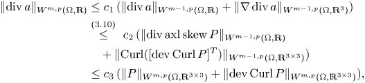 \begin{align*}
\lVert{\operatorname{div}
a}\rVert_{W^{m,p}(\Omega,\mathbb{R})} &\le
c_1\,(\lVert{\operatorname{div}
a}\rVert_{W^{m-1,p}(\Omega,\mathbb{R})}+ \lVert{\nabla
\operatorname{div}
a}\rVert_{W^{m-1,p}(\Omega,\mathbb{R}^{3})})\nonumber\\
&\stackrel{(3.10)}{\le} \ c_2 \,(\lVert{\operatorname{div}
\operatorname{axl}\operatorname{skew}
P}\rVert_{W^{m-1,p}(\Omega,\mathbb{R})}\notag\\
&\quad +
\lVert{\operatorname{Curl}([\operatorname{dev}\operatorname{Curl}
P]^{T})}\rVert_{W^{m-1,p}(\Omega,\mathbb{R}^{3\times 3})})\notag\\
&\le c_3
\,(\lVert{P}\rVert_{W^{m,p}(\Omega,\mathbb{R}^{3\times
3})}+ \lVert{\operatorname{dev}\operatorname{Curl}
P}\rVert_{W^{m,p}(\Omega,\mathbb{R}^{3\times 3})}),
\nonumber \end{align*}
\begin{align*}
\lVert{\operatorname{div}
a}\rVert_{W^{m,p}(\Omega,\mathbb{R})} &\le
c_1\,(\lVert{\operatorname{div}
a}\rVert_{W^{m-1,p}(\Omega,\mathbb{R})}+ \lVert{\nabla
\operatorname{div}
a}\rVert_{W^{m-1,p}(\Omega,\mathbb{R}^{3})})\nonumber\\
&\stackrel{(3.10)}{\le} \ c_2 \,(\lVert{\operatorname{div}
\operatorname{axl}\operatorname{skew}
P}\rVert_{W^{m-1,p}(\Omega,\mathbb{R})}\notag\\
&\quad +
\lVert{\operatorname{Curl}([\operatorname{dev}\operatorname{Curl}
P]^{T})}\rVert_{W^{m-1,p}(\Omega,\mathbb{R}^{3\times 3})})\notag\\
&\le c_3
\,(\lVert{P}\rVert_{W^{m,p}(\Omega,\mathbb{R}^{3\times
3})}+ \lVert{\operatorname{dev}\operatorname{Curl}
P}\rVert_{W^{m,p}(\Omega,\mathbb{R}^{3\times 3})}),
\nonumber \end{align*}
provided that 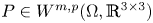 $P\in W^{m,p}(\Omega ,\mathbb {R}^{3\times 3})$. Together with (3.11) we conclude:
 \begin{equation} \lVert{\operatorname{Curl} P}\rVert_{W^{m,p}(\Omega,\mathbb{R}^{3\times 3})} \le c_4\, (\lVert{P}\rVert_{W^{m,p}(\Omega,\mathbb{R}^{3\times 3})}+ \lVert{\operatorname{dev}\operatorname{Curl} P}\rVert_{W^{m,p}(\Omega,\mathbb{R}^{3\times 3})})\end{equation}
as well as
 \begin{align} \lVert{P}\rVert_{W^{m,p}(\Omega,\mathbb{R}^{3\times 3})} &+\lVert{\operatorname{Curl} P}\rVert_{W^{m,p}(\Omega,\mathbb{R}^{3\times 3})}\nonumber\\ &\le c_5\, (\lVert{P}\rVert_{W^{m,p}(\Omega,\mathbb{R}^{3\times 3})}+ \lVert{\operatorname{dev}\operatorname{Curl} P}\rVert_{W^{m,p}(\Omega,\mathbb{R}^{3\times 3})}) \end{align}
and especially for  $m=0$:
 \begin{equation} \lVert{P}\rVert_{L^{p}(\Omega,\mathbb{R}^{3\times 3})} + \lVert{\operatorname{Curl} P}\rVert_{L^{p}(\Omega,\mathbb{R}^{3\times 3})} \le c_5\, (\lVert{P}\rVert_{L^{p}(\Omega,\mathbb{R}^{3\times 3})}+ \lVert{\operatorname{dev}\operatorname{Curl} P}\rVert_{L^{p}(\Omega,\mathbb{R}^{3\times 3})}) \end{equation}
for all  $P\in W^{1,p}(\operatorname {Curl};\Omega ,\mathbb {R}^{3\times 3})$.Footnote 6
Remark 17 The last identity in (3.11), which could also be formally obtained from (2.8) with  $b=-\nabla$, together with the expression (3.10) gives for general matrix field
  $P\in \mathscr {D}'(\Omega ,\mathbb {R}^{3\times 3})$:
 \begin{equation} \operatorname{D}\hspace{-1pt} \operatorname{Curl} P = L(\operatorname{D}\hspace{-1pt}\, \operatorname{dev} \operatorname{Curl} P). \end{equation}
Thus, recalling (1.7), we arrive directly at the case (b) of lemma 6.
Corollary 18 Notably, the trace condition in 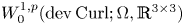 $W^{1,p}_ {0}(\operatorname {dev}\operatorname {Curl}; \Omega ,\mathbb {R}^{3\times 3})$ would read
  $\operatorname {dev} (P\times \nu ) = 0$ on
  $\partial \Omega ,$ to be understood by partial integration via
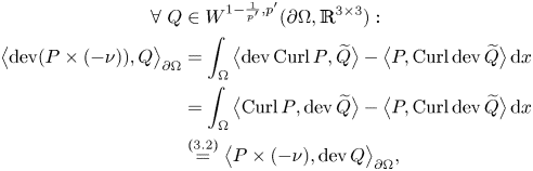 \begin{align} \forall\ Q&\in W^{1-\frac{1}{p'},p'}(\partial\Omega,\mathbb{R}^{3\times 3}): \nonumber\\ \big\langle{\operatorname{dev}(P\times (-\nu))},{Q}\big\rangle_{\partial \Omega} &= \int_{\Omega}\big\langle{\operatorname{dev}\operatorname{Curl} P},{\widetilde{Q}}\big\rangle-\big\langle{P},{\operatorname{Curl}\operatorname{dev} \widetilde{Q}}\big\rangle\, \mathrm{d}{x}\\ & = \int_{\Omega}\big\langle{\operatorname{Curl} P},{\operatorname{dev}\widetilde{Q}}\big\rangle-\big\langle{P},{\operatorname{Curl}\operatorname{dev} \widetilde{Q}}\big\rangle\, \mathrm{d}{x} \nonumber\\ & \overset{(3.2)}{=} \big\langle{P\times (-\nu)},{\operatorname{dev} Q}\big\rangle_{\partial \Omega}, \nonumber \end{align}
where  $\widetilde {Q}\in W^{1,p'}(\Omega ,\mathbb {R}^{3\times 3})$ denotes any extension of
  $Q$ in
  $\Omega$. However, it follows from observation 3 that the boundary conditions
  $P\times \nu = 0$ and
  $\operatorname {dev}(P\times \nu )=0$ on
  $\partial \Omega$ are the same.
Lemma 19 Let  $\Omega \subset \mathbb {R}^{3}$ be a bounded Lipschitz domain,
  $1< p<\infty$ and
  $P\in \mathscr {D}'(\Omega ,\mathbb {R}^{3\times 3})$. Then either of the conditions
(a)
$\operatorname {dev}\operatorname {sym} P\in L^{p}(\Omega ,\mathbb {R}^{3\times 3})$ and $\operatorname {Curl} P \in W^{-1,\ p}(\Omega ,\mathbb {R}^{3\times 3}),$(b)
$\operatorname {sym} P\in L^{p}(\Omega ,\mathbb {R}^{3\times 3})$ and $\operatorname {dev}\operatorname {Curl} P \in W^{-1,\ p}(\Omega ,\mathbb {R}^{3\times 3}),$(c)
$\operatorname {dev}\operatorname {sym} P\in L^{p}(\Omega ,\mathbb {R}^{3\times 3})$ and $\operatorname {dev}\operatorname {Curl} P \in W^{-1,p}(\Omega ,\mathbb {R}^{3\times 3}),$


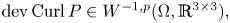
implies  $P\in L^{p}(\Omega ,\mathbb {R}^{3\times 3})$. Moreover, we have the corresponding estimates
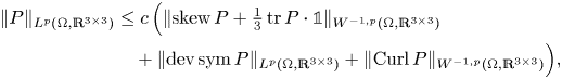 \begin{align} \lVert{P}\rVert_{L^{p}(\Omega,\mathbb{R}^{3\times 3})} &\leq c\, \Big(\lVert{\operatorname{skew} P+\textstyle\frac 13\operatorname{tr} P\cdot {\mathbb{1}}}\rVert_{W^{{-}1,p}(\Omega,\mathbb{R}^{3\times 3})}\nonumber\\ &\quad+ \lVert{\operatorname{dev}\operatorname{sym} P}\rVert_{L^{p}(\Omega,\mathbb{R}^{3\times 3})}+ \lVert{ \operatorname{Curl} P }\rVert_{W^{{-}1,p}(\Omega,\mathbb{R}^{3\times 3})}\Big),\end{align}
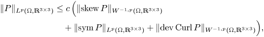 \begin{align}\lVert{P}\rVert_{L^{p}(\Omega,\mathbb{R}^{3\times 3})} &\leq c\, \Big(\lVert{\operatorname{skew} P}\rVert_{W^{{-}1,p}(\Omega,\mathbb{R}^{3\times 3})}\nonumber\\ &\quad+ \lVert{\operatorname{sym} P}\rVert_{L^{p}(\Omega,\mathbb{R}^{3\times 3})}+ \lVert{\operatorname{dev} \operatorname{Curl} P }\rVert_{W^{{-}1,p}(\Omega,\mathbb{R}^{3\times 3})}\Big),\end{align}
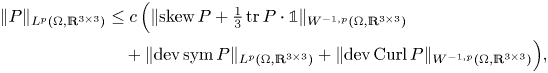 \begin{align} \lVert{P}\rVert_{L^{p}(\Omega,\mathbb{R}^{3\times 3})} &\leq c\, \Big(\lVert{\operatorname{skew} P+\textstyle\frac 13\operatorname{tr} P\cdot {\mathbb{1}}}\rVert_{W^{{-}1,p}(\Omega,\mathbb{R}^{3\times 3})}\notag\\ &\quad+ \lVert{\operatorname{dev}\operatorname{sym} P}\rVert_{L^{p}(\Omega,\mathbb{R}^{3\times 3})}+ \lVert{\operatorname{dev} \operatorname{Curl} P }\rVert_{W^{{-}1,p}(\Omega,\mathbb{R}^{3\times 3})}\Big), \end{align}
each with a constant  $c=c(p,\Omega )>0$.
Proof. We start by proving part (b). For that purpose we will follow the proof of [Reference Lewintan and Neff43, lemma 3.1]. Thus, for part (b) it remains to deduce that  $\operatorname {skew} P\in L^{p}(\Omega ,\mathbb {R}^{3\times 3})$. We have
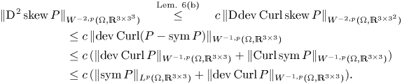 \begin{align} \lVert{\operatorname{D}\hspace{-1pt}^{2}\operatorname{skew} P}\rVert&_{W^{{-}2,p}(\Omega,\mathbb{R}^{ {3\times 3^{3}}})}\quad\overset{\text{Lem. 6(b)}}{\le}\quad c\, \lVert{\operatorname{D}\hspace{-1pt} \operatorname{dev} \operatorname{Curl}\operatorname{skew} P}\rVert_{W^{{-}2,p}(\Omega,\mathbb{R}^{ {3\times 3^{2}}})}\nonumber\\ &\le c\, \lVert{\operatorname{dev} \operatorname{Curl}(P-\operatorname{sym} P)}\rVert_{W^{{-}1,p}(\Omega,\mathbb{R}^{3\times 3})}\nonumber\\ & \le c\,( \lVert{\operatorname{dev} \operatorname{Curl} P }\rVert_{W^{{-}1,p}(\Omega,\mathbb{R}^{3\times 3})} + \lVert{\operatorname{Curl} \operatorname{sym} P}\rVert_{W^{{-}1,p}(\Omega,\mathbb{R}^{3\times 3})})\nonumber\\ & \le c\,( \lVert{\operatorname{sym} P}\rVert_{L^{p}(\Omega,\mathbb{R}^{3\times 3})}+ \lVert{\operatorname{dev} \operatorname{Curl} P }\rVert_{W^{{-}1,p}(\Omega,\mathbb{R}^{3\times 3})}). \end{align}
Hence, the assumptions of part (b) yield 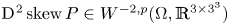 $\operatorname {D}\hspace {-1pt}^{2}\operatorname {skew} P\in W^{-2,p}(\Omega ,\mathbb {R}^{ {3\times 3^{3}}})$, so that, by corollary 9, we obtain
 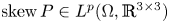 $\operatorname {skew} P\in L^{p}(\Omega ,\mathbb {R}^{3\times 3})$ and moreover the estimate
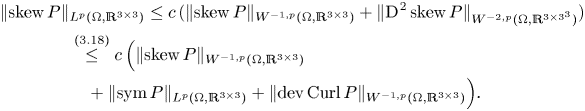 \begin{align} \lVert{\operatorname{skew} P}\rVert&_{L^{p}(\Omega,\mathbb{R}^{3\times 3})} \leq c\, (\lVert{\operatorname{skew} P}\rVert_{W^{{-}1,p}(\Omega,\mathbb{R}^{3\times 3})}+\lVert{\operatorname{D}\hspace{-1pt}^{2}\operatorname{skew} P}\rVert_{W^{{-}2,p}(\Omega,\mathbb{R}^{ {3\times 3^{3}}})})\nonumber\\ & \overset{(3.18)}{\le}c\, \Big(\lVert{\operatorname{skew} P}\rVert_{W^{{-}1,p}(\Omega,\mathbb{R}^{3\times 3})}\nonumber\\ &\quad+ \lVert{\operatorname{sym} P}\rVert_{L^{p}(\Omega,\mathbb{R}^{3\times 3})}+ \lVert{\operatorname{dev} \operatorname{Curl} P }\rVert_{W^{{-}1,p}(\Omega,\mathbb{R}^{3\times 3})}\Big). \end{align}
Then by adding 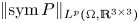 $\lVert {\operatorname {sym} P}\rVert _{L^{p}(\Omega ,\mathbb {R}^{3\times 3})}$ on both sides we obtain (3.17b).
Clearly, the conclusion of (a) as well as the estimate (3.17a) follow from (c) and (3.17c), respectively. To establish (c), we make use of the orthogonal decomposition  $P = \operatorname {dev}\operatorname {sym} P + (\operatorname {skew} P + \textstyle \frac 13\operatorname {tr} P \cdot {\mathbb{1}})$. Then, to obtain
  $\operatorname {skew} P + \textstyle \frac 13\operatorname {tr} P \cdot {\mathbb{1}}\in L^{p}(\Omega ,\mathbb {R}^{3\times 3})$ for (c), we consider
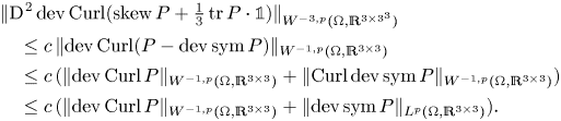 \begin{align} &\lVert{\operatorname{D}\hspace{-1pt}^{2}\operatorname{dev}\operatorname{Curl} (\operatorname{skew} P+ \textstyle\frac 13\operatorname{tr} P \cdot {\mathbb{1}})}\rVert_{ W^{{-}3,p}(\Omega,\mathbb{R}^{3\times 3^{3}})} \nonumber\\ &\quad\leq c\, \lVert{\operatorname{dev}\operatorname{Curl} (P-\operatorname{dev}\operatorname{sym} P)}\rVert_{ W^{{-}1,p}(\Omega,\mathbb{R}^{3\times 3})}\nonumber\\ &\quad\le c\,(\lVert{\operatorname{dev}\operatorname{Curl} P}\rVert_{ W^{{-}1,p}(\Omega,\mathbb{R}^{3\times 3})} + \lVert{\operatorname{Curl} \operatorname{dev}\operatorname{sym} P}\rVert_{ W^{{-}1,p}(\Omega,\mathbb{R}^{3\times 3})}) \nonumber\\ &\quad\leq c \,(\lVert{\operatorname{dev}\operatorname{Curl} P}\rVert_{ W^{{-}1,p}(\Omega,\mathbb{R}^{3\times 3})} + \lVert{\operatorname{dev}\operatorname{sym} P}\rVert_{ L^{p}(\Omega,\mathbb{R}^{3\times 3})}). \end{align}
Therefore,  $\operatorname {D}\hspace {-1pt}^{2}\operatorname {dev}\operatorname {Curl} (\operatorname {skew} P+ \textstyle \frac 13\operatorname {tr} P \cdot {\mathbb{1}})\in W^{-3,p}(\Omega ,\mathbb {R}^{3\times 3^{3}})$ follows from the assumptions of (c) and lemma 6(c) implies
 \begin{equation} \operatorname{D}\hspace{-1pt}^{3} (\operatorname{skew} P+ \textstyle\frac 13\operatorname{tr} P \cdot {\mathbb{1}})\in W^{{-}3,p}(\Omega,\mathbb{R}^{3\times 3^{4}}).\end{equation}
Applying corollary 9 again, this time to  $\operatorname {skew} P+ \textstyle \frac 13\operatorname {tr} P \cdot {\mathbb{1}}$, we arrive at
  $\operatorname {skew} P + \textstyle \frac 13\operatorname {tr} P \cdot {\mathbb{1}}\in L^{p}(\Omega ,\mathbb {R}^{3\times 3})$ and, moreover,
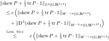 \begin{align}
&\lVert{\operatorname{skew} P+\textstyle\frac
13\operatorname{tr} P \cdot
{\mathbb{1}}}\rVert_{L^{p}(\Omega,\mathbb{R}^{3\times
3})}\notag\\
&\quad \le c\, \Big(\lVert{\operatorname{skew}
P+\textstyle\frac 13\operatorname{tr} P\cdot
{\mathbb{1}}}\rVert_{W^{{-}1,p}(\Omega,\mathbb{R}^{3\times
3})}\nonumber\\ &\qquad +
\lVert{\operatorname{D}\hspace{-1pt}^{3}(\operatorname{skew}
P+\textstyle\frac 13\operatorname{tr} P\cdot
{\mathbb{1}})}\rVert_{W^{{-}3,p}(\Omega,\mathbb{R}^{3\times
3^{4}})} \Big)\nonumber\\ &\quad \overset{\text{Lem.
6(c)}}{\leq}\quad c\,\Big(\lVert{\operatorname{skew}
P+\textstyle\frac 13\operatorname{tr} P\cdot
{\mathbb{1}}}\rVert_{W^{{-}1,p}(\Omega,\mathbb{R}^{3\times
3})}\\ &\qquad+
\lVert{\operatorname{D}\hspace{-1pt}^{2}\operatorname{dev}\operatorname{Curl}(\operatorname{skew}
P+\textstyle\frac 13\operatorname{tr} P\cdot
{\mathbb{1}})}\rVert_{W^{{-}3,p}(\Omega,\mathbb{R}^{3\times
3^{3}})} \Big)\nonumber\\ &\quad \overset{(3.20)}{\leq} \ c\,
\Big(\lVert{\operatorname{skew} P+\textstyle\frac
13\operatorname{tr} P\cdot
{\mathbb{1}}}\rVert_{W^{{-}1,p}(\Omega,\mathbb{R}^{3\times
3})}\nonumber\\ &\qquad +
\lVert{\operatorname{dev}\operatorname{sym}
P}\rVert_{L^{p}(\Omega,\mathbb{R}^{3\times 3})}+ \lVert{
\operatorname{dev}\operatorname{Curl} P
}\rVert_{W^{{-}1,p}(\Omega,\mathbb{R}^{3\times
3})}\Big).\nonumber \end{align}
\begin{align}
&\lVert{\operatorname{skew} P+\textstyle\frac
13\operatorname{tr} P \cdot
{\mathbb{1}}}\rVert_{L^{p}(\Omega,\mathbb{R}^{3\times
3})}\notag\\
&\quad \le c\, \Big(\lVert{\operatorname{skew}
P+\textstyle\frac 13\operatorname{tr} P\cdot
{\mathbb{1}}}\rVert_{W^{{-}1,p}(\Omega,\mathbb{R}^{3\times
3})}\nonumber\\ &\qquad +
\lVert{\operatorname{D}\hspace{-1pt}^{3}(\operatorname{skew}
P+\textstyle\frac 13\operatorname{tr} P\cdot
{\mathbb{1}})}\rVert_{W^{{-}3,p}(\Omega,\mathbb{R}^{3\times
3^{4}})} \Big)\nonumber\\ &\quad \overset{\text{Lem.
6(c)}}{\leq}\quad c\,\Big(\lVert{\operatorname{skew}
P+\textstyle\frac 13\operatorname{tr} P\cdot
{\mathbb{1}}}\rVert_{W^{{-}1,p}(\Omega,\mathbb{R}^{3\times
3})}\\ &\qquad+
\lVert{\operatorname{D}\hspace{-1pt}^{2}\operatorname{dev}\operatorname{Curl}(\operatorname{skew}
P+\textstyle\frac 13\operatorname{tr} P\cdot
{\mathbb{1}})}\rVert_{W^{{-}3,p}(\Omega,\mathbb{R}^{3\times
3^{3}})} \Big)\nonumber\\ &\quad \overset{(3.20)}{\leq} \ c\,
\Big(\lVert{\operatorname{skew} P+\textstyle\frac
13\operatorname{tr} P\cdot
{\mathbb{1}}}\rVert_{W^{{-}1,p}(\Omega,\mathbb{R}^{3\times
3})}\nonumber\\ &\qquad +
\lVert{\operatorname{dev}\operatorname{sym}
P}\rVert_{L^{p}(\Omega,\mathbb{R}^{3\times 3})}+ \lVert{
\operatorname{dev}\operatorname{Curl} P
}\rVert_{W^{{-}1,p}(\Omega,\mathbb{R}^{3\times
3})}\Big).\nonumber \end{align}□
Remark 20 Of course, part (a) can also be proven independently of part (c). Indeed, using lemma 6(a) we obtain
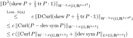 \begin{align}
&\lVert{\operatorname{D}\hspace{-1pt}^{2}(\operatorname{skew}
P+\textstyle\frac 13\operatorname{tr} P\cdot
{\mathbb{1}})}\rVert_{W^{{-}2,p}(\Omega,\mathbb{R}^{
{3\times 3^{3}}})}\nonumber\\ &\quad\overset{\text{Lem.
6(a)}}{\leq}\quad c\,
\lVert{\operatorname{D}\hspace{-1pt}\operatorname{Curl}
(\operatorname{skew} P+ \textstyle\frac 13\operatorname{tr}
P \cdot {\mathbb{1}})}\rVert_{
W^{{-}2,p}(\Omega,\mathbb{R}^{ {3\times
3^{2}}})}\nonumber\\ &\quad\leq c\,
\lVert{\operatorname{Curl}(P-\operatorname{dev}\operatorname{sym}
P)}\rVert_{ W^{{-}1,p}(\Omega,\mathbb{R}^{3\times 3})}
\nonumber\\ &\quad\leq c \,(\lVert{\operatorname{Curl}
P}\rVert_{ W^{{-}1,p}(\Omega,\mathbb{R}^{3\times 3})} +
\lVert{\operatorname{dev}\operatorname{sym} P}\rVert_{
L^{p}(\Omega,\mathbb{R}^{3\times 3})})
\end{align}
\begin{align}
&\lVert{\operatorname{D}\hspace{-1pt}^{2}(\operatorname{skew}
P+\textstyle\frac 13\operatorname{tr} P\cdot
{\mathbb{1}})}\rVert_{W^{{-}2,p}(\Omega,\mathbb{R}^{
{3\times 3^{3}}})}\nonumber\\ &\quad\overset{\text{Lem.
6(a)}}{\leq}\quad c\,
\lVert{\operatorname{D}\hspace{-1pt}\operatorname{Curl}
(\operatorname{skew} P+ \textstyle\frac 13\operatorname{tr}
P \cdot {\mathbb{1}})}\rVert_{
W^{{-}2,p}(\Omega,\mathbb{R}^{ {3\times
3^{2}}})}\nonumber\\ &\quad\leq c\,
\lVert{\operatorname{Curl}(P-\operatorname{dev}\operatorname{sym}
P)}\rVert_{ W^{{-}1,p}(\Omega,\mathbb{R}^{3\times 3})}
\nonumber\\ &\quad\leq c \,(\lVert{\operatorname{Curl}
P}\rVert_{ W^{{-}1,p}(\Omega,\mathbb{R}^{3\times 3})} +
\lVert{\operatorname{dev}\operatorname{sym} P}\rVert_{
L^{p}(\Omega,\mathbb{R}^{3\times 3})})
\end{align}
and the conclusion follows from an application of corollary 9 to  $\operatorname {skew} P+ \textstyle \frac 13\operatorname {tr} P \cdot {\mathbb{1}}$.
The rigidity results now follow by elimination of the corresponding first term on the right-hand side.
Theorem 21 Let  $\Omega \subset \mathbb {R}^{3}$ be a bounded Lipschitz domain and
  $1< p<\infty$. There exists a constant
  $c=c(p,\Omega )>0$ such that for all
  $P\in { L^{p}}(\Omega ,\mathbb {R}^{3\times 3})$ we have
 \begin{align}
&\inf_{T\in
K_{dS,C}}\lVert{P-T}\rVert_{L^{p}(\Omega,\mathbb{R}^{3\times
3})}\nonumber\\ &\quad \leq c\,\left(\lVert{\operatorname{dev}
\operatorname{sym} P
}\rVert_{L^{p}(\Omega,\mathbb{R}^{3\times 3})}+ \lVert{
\operatorname{Curl} P
}\rVert_{W^{{-}1,p}(\Omega,\mathbb{R}^{3\times
3})}\right),\end{align}
\begin{align}
&\inf_{T\in
K_{dS,C}}\lVert{P-T}\rVert_{L^{p}(\Omega,\mathbb{R}^{3\times
3})}\nonumber\\ &\quad \leq c\,\left(\lVert{\operatorname{dev}
\operatorname{sym} P
}\rVert_{L^{p}(\Omega,\mathbb{R}^{3\times 3})}+ \lVert{
\operatorname{Curl} P
}\rVert_{W^{{-}1,p}(\Omega,\mathbb{R}^{3\times
3})}\right),\end{align} \begin{align}&\inf_{T\in
K_{S,dC}}\lVert{P-T}\rVert_{L^{p}(\Omega,\mathbb{R}^{3\times
3})}\notag\\ &\quad \leq c\,\left(\lVert{\operatorname{sym} P
}\rVert_{L^{p}(\Omega,\mathbb{R}^{3\times 3})}+
\lVert{\operatorname{dev} \operatorname{Curl} P
}\rVert_{W^{{-}1,p}(\Omega,\mathbb{R}^{3\times
3})}\right),\end{align}
\begin{align}&\inf_{T\in
K_{S,dC}}\lVert{P-T}\rVert_{L^{p}(\Omega,\mathbb{R}^{3\times
3})}\notag\\ &\quad \leq c\,\left(\lVert{\operatorname{sym} P
}\rVert_{L^{p}(\Omega,\mathbb{R}^{3\times 3})}+
\lVert{\operatorname{dev} \operatorname{Curl} P
}\rVert_{W^{{-}1,p}(\Omega,\mathbb{R}^{3\times
3})}\right),\end{align}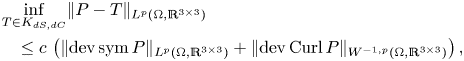 \begin{align}&\inf_{T\in
K_{dS,dC}}\lVert{P-T}\rVert_{L^{p}(\Omega,\mathbb{R}^{3\times
3})}\notag\\
&\quad \leq c\,\left(\lVert{\operatorname{dev}
\operatorname{sym} P
}\rVert_{L^{p}(\Omega,\mathbb{R}^{3\times 3})}+
\lVert{\operatorname{dev} \operatorname{Curl} P
}\rVert_{W^{{-}1,p}(\Omega,\mathbb{R}^{3\times
3})}\right),
\end{align}
\begin{align}&\inf_{T\in
K_{dS,dC}}\lVert{P-T}\rVert_{L^{p}(\Omega,\mathbb{R}^{3\times
3})}\notag\\
&\quad \leq c\,\left(\lVert{\operatorname{dev}
\operatorname{sym} P
}\rVert_{L^{p}(\Omega,\mathbb{R}^{3\times 3})}+
\lVert{\operatorname{dev} \operatorname{Curl} P
}\rVert_{W^{{-}1,p}(\Omega,\mathbb{R}^{3\times
3})}\right),
\end{align}where the kernels are given, respectively, by
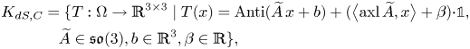 \begin{align} K_{dS,C}&=\{T:\Omega\to\mathbb{R}^{3\times 3}\mid T(x)=\operatorname{Anti}(\widetilde{A}\,x+b)+(\big\langle{\operatorname{axl} \widetilde{A}},{x}\big\rangle+\beta) {\cdot}{\mathbb{1}}, \notag\\ &\quad\widetilde{A}\in\mathfrak{so}(3), b\in\mathbb{R}^{3}, \beta\in\mathbb{R} \} {,} \end{align}
 \begin{align} K_{S,dC} &= \{T:\Omega\to\mathbb{R}^{3\times 3}\mid T(x)=\operatorname{Anti}(\beta\,x+b), \ b\in\mathbb{R}^{3}, \beta\in\mathbb{R}\}, \end{align}
 \begin{align} K_{dS,dC} &= \{T:\Omega\to\mathbb{R}^{3\times 3}\mid T(x)=\operatorname{Anti}\big(\widetilde{A}\,x+\beta\, x+b \big)+\big(\big\langle{\operatorname{axl}\widetilde{A}},{x}\big\rangle+\gamma \big) {\cdot}{\mathbb{1}}, \notag\\&\widetilde{A}\in\mathfrak{so}(3), b\in\mathbb{R}^{3}, \beta,\gamma\in\mathbb{R}\}. \end{align}
Proof. We proceed as in the proof of Korn's inequalities (1.4) resp. (1.5), see [Reference Lewintan and Neff43, theorem 3.3] resp. [Reference Ciarlet12, theorem 6.15-3], and start by characterizing the kernel of the right-hand side,
 \begin{align*} K_{dS,C} : = \{P\in { L^{p}}(\Omega,\mathbb{R}^{3\times 3}) \mid \ & \operatorname{dev} \operatorname{sym} P = 0 \text{ a.e. and }\\ & \operatorname{Curl} P= 0 \text{ in the distributional sense}\}, \end{align*}
so that  $P\in K_{dS,C}$ if and only if
  $P=\operatorname {skew} P + \frac 13\operatorname {tr} P\cdot {\mathbb{1}}$ and
  $\operatorname {Curl}(\operatorname {skew} P + \frac 13\operatorname {tr}P\cdot {\mathbb{1}})\equiv 0$. Hence, (3.25a) follows by virtue of Lemma 11(a).
Let us denote by  $e_1,\ldots ,e_M$ a basis of
  $K_{dS,C}$, where
  $M: = \dim K_{dS,C} = 7$, and by
  $\ell _1, \ldots , \ell _M$ the corresponding continuous linear forms on
  $K_{dS,C}$ given by
 \begin{equation} \ell_\alpha(e_j): = \delta_{\alpha j}. \end{equation}
By the Hahn-Banach theorem in a normed vector space (see e.g. [Reference Ciarlet12, theorem 5.9-1]), we extend  $\ell _\alpha$ to continuous linear forms—again denoted by
  $\ell _\alpha$—on the Banach space
  ${ L^{p}}(\Omega ,\mathbb {R}^{3\times 3})$,
  $1\le \alpha \le M$. Notably,
 \[ T\in K_{dS,C} \text{ is equal to }0 \quad \Leftrightarrow \quad \ell_\alpha(T)= 0 \ \forall\ \alpha\in\{1,\ldots,M\}. \]
Following the proof of [Reference Lewintan and Neff43, theorem 3.4] we eliminate the first term on the right-hand side of (3.17a) by exploiting the compactness  $L^{p}(\Omega ,\mathbb {R}^{3\times 3})\subset \!\subset W^{-1,p}(\Omega ,\mathbb {R}^{3\times 3})$ and arrive at
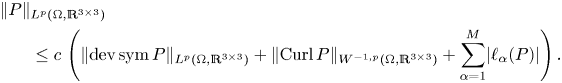 \begin{align} \lVert{P}\rVert&_{L^{p}(\Omega,\mathbb{R}^{3\times 3})}\nonumber\\ &\leq c\,\left(\lVert{\operatorname{dev} \operatorname{sym} P }\rVert_{L^{p}(\Omega,\mathbb{R}^{3\times 3})}+ \lVert{ \operatorname{Curl} P }\rVert_{W^{{-}1,p}(\Omega,\mathbb{R}^{3\times 3})}+\sum_{\alpha=1}^{M}\lvert{\ell_\alpha(P)}\rvert \right). \end{align}
Indeed, if (3.27) were false, there would exist a sequence  $P_k\in L^{p}(\Omega ,\mathbb {R}^{3\times 3})$ such that
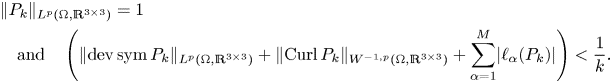 \begin{align*} &\lVert{P_k}\rVert_{L^{p}(\Omega,\mathbb{R}^{3\times 3})}=1 \\ &\quad \text{and}\quad \left(\lVert{\operatorname{dev} \operatorname{sym} P_k }\rVert_{L^{p}(\Omega,\mathbb{R}^{3\times 3})}+ \lVert{ \operatorname{Curl} P_k }\rVert_{W^{{-}1,p}(\Omega,\mathbb{R}^{3\times 3})}+\sum_{\alpha=1}^{M}\lvert{\ell_\alpha(P_k)}\rvert \right)<\frac{1}{k}. \end{align*}
Thus, for a subsequence  $P_k\rightharpoonup P^{*}$ in
  $L^{p}(\Omega ,\mathbb {R}^{3\times 3}$ with
  $\operatorname {dev}\operatorname {sym} P^{*}=0$ a.e.,
  $\operatorname {sym} \operatorname {Curl} P^{*}=0$ in the distributional sense and
  $\ell _\alpha (P_k)=0$ for all
  $\alpha =1,\ldots ,M$, so that
  $P^{*}=0$ a.e.. By the compact embedding
  $L^{p}(\Omega ,\mathbb {R}^{3\times 3})\subset \!\subset W^{-1,p}(\Omega ,\mathbb {R}^{3\times 3})$ there exists a subsequence
  $P_k$, so that
  $\operatorname {skew} P_k+\frac 13\operatorname {tr} P_k\cdot {\mathbb{1}}\to 0$ in
  $W^{-1,p}(\Omega ,\mathbb {R}^{3\times 3})$. This is a contradiction to (3.17a).
Considering now the projection  $\pi _{a}:{ L^{p}}(\Omega ,\mathbb {R}^{3\times 3}) \to K_{dS,C}$ given by
 \begin{equation} \pi_{a}(P): = \sum_{j=1}^{M} \ell_j(P)\, e_j \end{equation}
we obtain  $\ell _\alpha (P-\pi _{a}(P)) \overset{(3.26)}{=} 0$ for all
  $1\le \alpha \le M$, so that (3.24a) follows after applying (3.27) to
  $P-\pi _{a}(P)$.
Furthermore, we obtain the characterizations (3.25b) and (3.25c) by lemma 11 (b) and (c), respectively, since
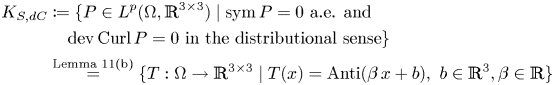 \begin{align} K_{S,dC} &: = \{P\in { L^{p}}(\Omega,\mathbb{R}^{3\times 3}) \mid \operatorname{sym} P = 0 \text{ a.e. and } \nonumber\\ &\quad\operatorname{dev}\operatorname{Curl} P= 0 \text{ in the distributional sense}\}\\ &\overset{\text{Lemma 11(b)}}{=}\{T:\Omega\to\mathbb{R}^{3\times 3}\mid T(x)=\operatorname{Anti}(\beta\,x+b), \ b\in\mathbb{R}^{3}, \beta\in\mathbb{R}\}\end{align}
and
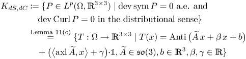 \begin{align}
K_{dS,dC} &: = \{P\in {
L^{p}}(\Omega,\mathbb{R}^{3\times 3}) \mid
\operatorname{dev}\operatorname{sym} P= 0 \text{ a.e. and
}\nonumber\\ &\quad \operatorname{dev}\operatorname{Curl}
P= 0 \text{ in the distributional sense}\}\\
&\overset{\text{Lemma
11(c)}}{=}\{T:\Omega\to\mathbb{R}^{3\times 3}\mid
T(x)=\operatorname{Anti}\big(\widetilde{A}\,x+\beta\, x+b
\big)\nonumber\\
&\quad+\big(\big\langle{\operatorname{axl}\widetilde{A}},{x}\big\rangle+\gamma
\big) {\cdot}{\mathbb{1}}, \widetilde{A}\in\mathfrak{so}(3),
b\in\mathbb{R}^{3}, \beta,\gamma\in\mathbb{R}\} \nonumber
\end{align}
\begin{align}
K_{dS,dC} &: = \{P\in {
L^{p}}(\Omega,\mathbb{R}^{3\times 3}) \mid
\operatorname{dev}\operatorname{sym} P= 0 \text{ a.e. and
}\nonumber\\ &\quad \operatorname{dev}\operatorname{Curl}
P= 0 \text{ in the distributional sense}\}\\
&\overset{\text{Lemma
11(c)}}{=}\{T:\Omega\to\mathbb{R}^{3\times 3}\mid
T(x)=\operatorname{Anti}\big(\widetilde{A}\,x+\beta\, x+b
\big)\nonumber\\
&\quad+\big(\big\langle{\operatorname{axl}\widetilde{A}},{x}\big\rangle+\gamma
\big) {\cdot}{\mathbb{1}}, \widetilde{A}\in\mathfrak{so}(3),
b\in\mathbb{R}^{3}, \beta,\gamma\in\mathbb{R}\} \nonumber
\end{align}
with  $\dim K_{S,dC}=4$ and
  $\dim K_{dS,dC}=8$. Hence, we can argue as above to deduce (3.24b) and (3.24c) from (3.17b) and (3.17c), respectively, since we end up with
 \begin{equation} \lVert{P-\pi_{b}(P)}\rVert_{L^{p}(\Omega,\mathbb{R}^{3\times 3})}\leq c\,\left(\lVert{\operatorname{sym} P }\rVert_{L^{p}(\Omega,\mathbb{R}^{3\times 3})}+ \lVert{\operatorname{dev} \operatorname{Curl} P }\rVert_{W^{{-}1,p}(\Omega,\mathbb{R}^{3\times 3})}\right) \end{equation}
and
 \begin{align} \lVert{P-\pi_{c}(P)}\rVert_{L^{p}(\Omega,\mathbb{R}^{3\times 3})}\leq c\,\left(\lVert{\operatorname{dev} \operatorname{sym} P }\rVert_{L^{p}(\Omega,\mathbb{R}^{3\times 3})}+ \lVert{\operatorname{dev} \operatorname{Curl} P }\rVert_{W^{{-}1,p}(\Omega,\mathbb{R}^{3\times 3})}\right)\end{align}
respectively, with projections  $\pi _{b}:{ L^{p}}(\Omega ,\mathbb {R}^{3\times 3}) \to K_{S,dC}$ and
  $\pi _{c}:{ L^{p}}(\Omega ,\mathbb {R}^{3\times 3}) \to K_{dS,dC}$.
Finally, the kernel is killed by the tangential trace condition  $P\times \nu \equiv 0$ (
 $\Leftrightarrow ~\operatorname {dev}(P\times \nu )=0$, cf. Obs. 3):
Theorem 22 Let  $\Omega \subset \mathbb {R}^{3}$ be a bounded Lipschitz domain and
  $1< p<\infty$. There exists a constant
  $c=c(p,\Omega )>0$ such that for all
  $P\in W^{1,p}_0(\operatorname {Curl}; \Omega ,\mathbb {R}^{3\times 3})$ we have
 \begin{equation} \lVert{ P }\rVert_{L^{p}(\Omega,\mathbb{R}^{3\times 3})}\leq c\,\left(\lVert{\operatorname{dev} \operatorname{sym} P }\rVert_{L^{p}(\Omega,\mathbb{R}^{3\times 3})}+ \lVert{ \operatorname{dev}\operatorname{Curl} P }\rVert_{L^{p}(\Omega,\mathbb{R}^{3\times 3})}\right).\end{equation}
Proof. We argue as in the proof of [Reference Lewintan and Neff43, theorem 3.5] and consider a sequence  $\{P_k\}_{k\in \mathbb {N}}\subset W^{1,p}_0(\operatorname {Curl};\Omega ,\mathbb {R}^{3\times 3})$ which converges weakly in
  $L^{p}(\Omega ,\mathbb {R}^{3\times 3})$ to
  $P^{*}$ so that
  $\operatorname {dev}\operatorname {sym} P^{*} = 0$ a.e. and
  $\operatorname {dev}\operatorname {Curl} P^{*}= 0$ in the distributional sense, i.e.
  $P^{*}\in K_{dS,dC}$, where
 \begin{align*}
K_{dS,dC} &\overset{(3.25c)}=
\{T:\Omega\to\mathbb{R}^{3\times 3}\mid
T(x)=\operatorname{Anti}\big(\widetilde{A}\,x+\beta\, x+b
\big)+\big(\big\langle{\operatorname{axl}\widetilde{A}},{x}\big\rangle+\gamma
\big) {\cdot}{\mathbb{1}}, \nonumber \\
&\quad\widetilde{A}\in\mathfrak{so}(3), b\in\mathbb{R}^{3},
\beta,\gamma\in\mathbb{R}\}. \end{align*}
\begin{align*}
K_{dS,dC} &\overset{(3.25c)}=
\{T:\Omega\to\mathbb{R}^{3\times 3}\mid
T(x)=\operatorname{Anti}\big(\widetilde{A}\,x+\beta\, x+b
\big)+\big(\big\langle{\operatorname{axl}\widetilde{A}},{x}\big\rangle+\gamma
\big) {\cdot}{\mathbb{1}}, \nonumber \\
&\quad\widetilde{A}\in\mathfrak{so}(3), b\in\mathbb{R}^{3},
\beta,\gamma\in\mathbb{R}\}. \end{align*}
By (3.16) it further follows that  $\big \langle {\operatorname {dev}(P^{*}\times (-\nu ))},{Q}\big \rangle _{\partial \Omega }=0$ for all
  $Q\in W^{1-\frac {1}{p'},p'}(\partial \Omega ,\mathbb {R}^{3\times 3})$. However, since
  $P^{*}\in K_{dS,dC}$ also has an explicit representation, the boundary condition
  $\operatorname {dev}(P^{*}\times \nu )=0$ is also valid in the classical sense. Furthermore, we deduce by observation 3 that
  $P^{*}\times \nu =0$ on
  $\partial \Omega$, so that
  $P^{*}\in W^{1,p}_0(\operatorname {Curl}; \Omega ,\mathbb {R}^{3\times 3})$. Again, using the explicit representation of
  $P^{*}=\operatorname {Anti}(\widetilde {A}\,x+\beta \, x +b)+(\big \langle {\operatorname {axl}\widetilde {A}},{x}\big \rangle +\gamma ) {\cdot }{\mathbb{1}}$, we conclude with Observation 4 that, in fact,
  $P^{*}\equiv 0$:
 \begin{align*} &[\operatorname{Anti}\big(\widetilde{A}\,x +\beta\, x+b \big)+\big(\big\langle{\operatorname{axl}\widetilde{A}},{x}\big\rangle+\gamma \big) {\cdot}{\mathbb{1}}] \times \nu = 0 \\ &\quad\overset{\text{Obs. 4}}{\Rightarrow} \quad \widetilde{A}\,x+\beta\, x+b =0 \quad \text{and} \quad \big\langle{\operatorname{axl}\widetilde{A}},{x}\big\rangle+\gamma=0 \quad \text{for all }x\in\partial\Omega\\ &\quad \Rightarrow\quad \gamma = 0, \ \widetilde{A}= 0 \quad \Rightarrow \quad b=0, \beta=0. \end{align*}
□
Remark 23 Similarly, the following estimates can also be deduced, even independently of (3.34), for  $P\in W^{1,p}_0(\operatorname {Curl}; \Omega ,\mathbb {R}^{3\times 3})$:
 \begin{align} \lVert{ P }\rVert_{L^{p}(\Omega,\mathbb{R}^{3\times 3})}&\leq c\,\left(\lVert{\operatorname{dev} \operatorname{sym} P }\rVert_{L^{p}(\Omega,\mathbb{R}^{3\times 3})}+ \lVert{ \operatorname{Curl} P }\rVert_{L^{p}(\Omega,\mathbb{R}^{3\times 3})}\right), \end{align}
 \begin{align} \lVert{ P }\rVert_{L^{p}(\Omega,\mathbb{R}^{3\times 3})}&\leq c\,\left(\lVert{\operatorname{sym} P }\rVert_{L^{p}(\Omega,\mathbb{R}^{3\times 3})}+ \lVert{ \operatorname{dev}\operatorname{Curl} P }\rVert_{L^{p}(\Omega,\mathbb{R}^{3\times 3})}\right). \end{align}
Since by [Reference Bauer, Neff, Pauly and Starke6, theorem 3.1 (ii)] it holds
 \begin{equation} \lVert{\operatorname{Curl} P}\rVert_{L^{p}(\Omega,\mathbb{R}^{3\times 3})}\leq c\, \lVert{\operatorname{dev} \operatorname{Curl} P }\rVert_{L^{p}(\Omega,\mathbb{R}^{3\times 3})} \qquad \text{for } P\in W^{1,p}_0(\operatorname{Curl};\Omega,\mathbb{R}^{3\times 3}), \end{equation}
we can recover (3.34) from (3.35) and (3.37).
However, without boundary conditions the Nečas estimate provides for  $P\in W^{1,p}(\operatorname {Curl}; \Omega ,\mathbb {R}^{3\times 3})$:
 \begin{align} \lVert{\operatorname{Curl} P}\rVert_{L^{p}(\Omega,\mathbb{R}^{3\times 3})} &\overset{(2.36)}{\le} c\, (\lVert{\operatorname{Curl} P}\rVert_{W^{{-}1,p}(\Omega,\mathbb{R}^{3\times 3})}+\lVert{\operatorname{D}\hspace{-1pt} \operatorname{Curl} P}\rVert_{W^{{-}1,p}(\Omega,\mathbb{R}^{ {3\times 3^{2}}})}) \nonumber\\ &\overset{(3.15)}{\le} c\, (\lVert{\operatorname{Curl} P}\rVert_{W^{{-}1,p}(\Omega,\mathbb{R}^{3\times 3})}+\lVert{\operatorname{D}\hspace{-1pt} \operatorname{dev}\operatorname{Curl} P}\rVert_{W^{{-}1,p}(\Omega,\mathbb{R}^{ {3\times 3^{2}}})}) \nonumber\\ & \le~ c\, (\lVert{\operatorname{Curl} P}\rVert_{W^{{-}1,p}(\Omega,\mathbb{R}^{3\times 3})}+\lVert{\operatorname{dev}\operatorname{Curl} P}\rVert_{L^{p}(\Omega,\mathbb{R}^{3\times 3})}). \end{align}
Remark 24 Among the inequalities (3.34), (3.35) and (3.36) we expect (3.35) also to hold true in higher space dimensions  $n>3$, see the discussion in our Introduction.
Remark 25 Regarding (3.14) and (3.34) or (3.37) and (3.34) we obtain the norm equivalence
 \begin{align*} \lVert{ P }\rVert_{L^{p}(\Omega,\mathbb{R}^{3\times 3})}+&\ \lVert{ \operatorname{Curl} P }\rVert_{L^{p}(\Omega,\mathbb{R}^{3\times 3})}\\ &\leq c\,\left(\lVert{\operatorname{dev} \operatorname{sym} P }\rVert_{L^{p}(\Omega,\mathbb{R}^{3\times 3})} + \lVert{ \operatorname{dev} \operatorname{Curl} P }\rVert_{L^{p}(\Omega,\mathbb{R}^{3\times 3})}\right) \end{align*}
for tensor fields  $P\in W^{1,p}_0(\operatorname {Curl}; \Omega ,\mathbb {R}^{3\times 3})$.
For  $P=\operatorname {D}\hspace {-1pt} u$ in (3.34) we recover the following tangential trace-free Korn inequality:
Corollary 26 Let  $\Omega \subset \mathbb {R}^{3}$ be a bounded Lipschitz domain and
  $1< p<\infty$. There exists a constant
  $c=c(p,\Omega )>0$ such that for all
  $u\in W^{1,p}(\Omega ,\mathbb {R}^{3})$ with
  $\operatorname {D}\hspace {-1pt} u \times \nu =0$ on
  $\partial \Omega$ we have
 \begin{equation} \lVert{ \operatorname{D}\hspace{-1pt} u }\rVert_{L^{p}(\Omega,\mathbb{R}^{3\times 3})}\leq c\,\lVert{\operatorname{dev} \operatorname{sym} \operatorname{D}\hspace{-1pt} u }\rVert_{L^{p}(\Omega,\mathbb{R}^{3\times 3})}.\end{equation}
 For skew-symmetric  $P=\operatorname {Anti}(a)$ we recover from (3.34) a Poincaré inequality involving only the deviatoric (trace-free) part of the gradient:
Corollary 27 Let  $\Omega \subset \mathbb {R}^{3}$ be a bounded Lipschitz domain and
  $1< p<\infty$. There exists a constant
  $c=c(p,\Omega )>0$ such that for all
  $a\in W^{1,p}_0(\Omega ,\mathbb {R}^{3})$ we have
 \begin{equation} \lVert{a}\rVert_{L^{p}(\Omega,\mathbb{R}^{3})}\leq c\,\lVert{\operatorname{dev} \operatorname{D}\hspace{-1pt} a }\rVert_{L^{p}(\Omega,\mathbb{R}^{3\times 3})}.\end{equation}
Proof. This follows from theorem 22 by setting  $P=\operatorname {Anti}(a)$ and the following observations:
 $\operatorname {Anti}(a)\times \nu =0 \ \Leftrightarrow \ a = 0$ on
  $\partial \Omega$, see observation 4,
  $\operatorname {Curl} (\operatorname {Anti}(a))=L(\operatorname {D}\hspace {-1pt} a)$, see (2.16a) and the form of
  $\operatorname {Anti}(a)$, see (2.2).
Remark 28 The previous results also hold true for functions with vanishing tangential trace only on a relatively open (non-empty) subset  $\Gamma \subseteq \partial \Omega$ of the boundary. So, e.g., we have
 \begin{equation} \lVert{ P }\rVert_{L^{p}(\Omega,\mathbb{R}^{3\times 3})}\leq c\,\left(\lVert{\operatorname{dev} \operatorname{sym} P }\rVert_{L^{p}(\Omega,\mathbb{R}^{3\times 3})}+ \lVert{ \operatorname{dev}\operatorname{Curl} P }\rVert_{L^{p}(\Omega,\mathbb{R}^{3\times 3})}\right) \end{equation}
for all  $P\in W^{1,p}_{\Gamma ,0}(\operatorname {Curl};\Omega ,\mathbb {R}^{3\times 3})$, which is the completion of
  $C^{\infty }_{\Gamma ,0}(\Omega ,\mathbb {R}^{3\times 3})$ with respect to the
  $W^{1,p}(\operatorname {Curl};\Omega ,\mathbb {R}^{3\times 3})$-norm.
Remark 29 In [Reference Garroni, Leoni and Ponsiglione28] the authors proved that in  $n=2$ dimensions, for
  $p=2$ a Korn inequality for incompatibile fields also holds true when
  $\operatorname {Curl} P$ is only in
  $L^{1}$ (actually when it is a measure with bounded total variation) under the normalization condition
  $\int _\Omega \operatorname {skew} P\,\mathrm {d}{x}=0$. In terms of scaling, it is interesting to involve in (3.34) the Sobolev exponent. So, we will show in a forthcoming paper that for
  $1< p<3$ the following estimate holds true on an arbitrary open set
  $\Omega \subseteq \mathbb {R}^{3}$:
 \begin{equation} \lVert{P}\rVert_{L^{p^{*}}(\Omega,\mathbb{R}^{3\times 3})}\le c\, (\lVert{\operatorname{dev}\operatorname{sym} P}\rVert_{L^{p^{*}}(\Omega,\mathbb{R}^{3\times 3})}+\lVert{\operatorname{dev}\operatorname{Curl} P}\rVert_{L^{p}(\Omega,\mathbb{R}^{3\times 3})})\end{equation}
for all  $P\in C^{\infty }_c(\Omega ,\mathbb {R}^{3\times 3})$, where
  $p^{*}=\frac {3p}{3-p}$. However, we do not know if such a result still holds in the borderline case
  $p=1$.
Acknowledgments
The authors are grateful for inspiring discussions with Stefan Müller (Hausdorff Center for Mathematics, Bonn, Germany) and thank also the anonymous referee for his valuable comments and suggestions. This work was initiated in the framework of the Priority Programme SPP 2256 ‘Variational Methods for Predicting Complex Phenomena in Engineering Structures and Materials’ funded by the Deutsche Forschungsgemeinschaft (DFG, German research foundation), Project-ID 422730790. The second author was supported within the project ’A variational scale-dependent transition scheme—from Cauchy elasticity to the relaxed micromorphic continuum’ (Project-ID 440935806). Moreover, both authors were supported in the Project-ID 41589 4848 by the Deutsche Forschungsgemeinschaft.
Appendix A. Appendix
Appendix A.1 On the trace-free Korn's first inequality in $L^{2}$

Using partial integration (see also [Reference Neff, Pauly and Witsch58, appendix A.1]) we catch up with a simple proof of
Lemma 30 Let  $n\ge 2$,
  $\Omega \ (\text {open})\subset \mathbb {R}^{n},$
  $u\in W^{1,2}_0(\Omega , \mathbb {R}^{n})$. Then
 \begin{equation} \int_\Omega \lVert{\operatorname{D}\hspace{-1pt} u}\rVert^{2} \mathrm{d}{x} \leq 2 \int_\Omega \lVert{\operatorname{dev}_n\operatorname{sym} \operatorname{D}\hspace{-1pt} u}\rVert^{2}\mathrm{d}{x}. \end{equation}
Proof. For 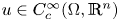 $u\in C^{\infty }_c(\Omega ,\mathbb {R}^{n})$ we have
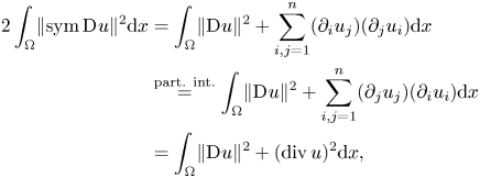 \begin{align} 2
\int_\Omega \lVert{\operatorname{sym}
\operatorname{D}\hspace{-1pt} u}\rVert^{2}\mathrm{d}{x} &=
\int_\Omega \lVert{\operatorname{D}\hspace{-1pt}
u}\rVert^{2} + \sum_{i,j=1}^{n}(\partial_i u_j)(\partial_j
u_i)\mathrm{d}{x}\notag\\
& \overset{\text{part. int.}}{=}\int_\Omega
\lVert{\operatorname{D}\hspace{-1pt} u}\rVert^{2} +
\sum_{i,j=1}^{n}(\partial_j u_j)(\partial_i
u_i)\mathrm{d}{x}\nonumber\\ & = \int_\Omega
\lVert{\operatorname{D}\hspace{-1pt} u}\rVert^{2} +
(\operatorname{div} u)^{2}\mathrm{d}{x},
\end{align}
\begin{align} 2
\int_\Omega \lVert{\operatorname{sym}
\operatorname{D}\hspace{-1pt} u}\rVert^{2}\mathrm{d}{x} &=
\int_\Omega \lVert{\operatorname{D}\hspace{-1pt}
u}\rVert^{2} + \sum_{i,j=1}^{n}(\partial_i u_j)(\partial_j
u_i)\mathrm{d}{x}\notag\\
& \overset{\text{part. int.}}{=}\int_\Omega
\lVert{\operatorname{D}\hspace{-1pt} u}\rVert^{2} +
\sum_{i,j=1}^{n}(\partial_j u_j)(\partial_i
u_i)\mathrm{d}{x}\nonumber\\ & = \int_\Omega
\lVert{\operatorname{D}\hspace{-1pt} u}\rVert^{2} +
(\operatorname{div} u)^{2}\mathrm{d}{x},
\end{align}
from where the ‘baby’ Korn inequality 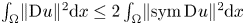 $\int _\Omega \lVert {\operatorname {D}\hspace {-1pt} u}\rVert ^{2} \mathrm {d}{x} \leq 2 \int _\Omega \lVert {\operatorname {sym} \operatorname {D}\hspace {-1pt} u}\rVert ^{2}\mathrm {d}{x}$ for
  $u\in W^{1,2}_0(\Omega , \mathbb {R}^{n})$ follows. Its improvement is obtained in regard with the decomposition
 \begin{equation} \lVert{\operatorname{dev}_n\operatorname{sym} \operatorname{D}\hspace{-1pt} u}\rVert^{2} = \lVert{\operatorname{sym} \operatorname{D}\hspace{-1pt} u - \frac 1n\underset{=\operatorname{div} u}{\underbrace{\operatorname{tr}(\operatorname{sym}\operatorname{D}\hspace{-1pt} u)}}\cdot{\mathbb{1}}}\rVert^{2} = \lVert{\operatorname{sym} \operatorname{D}\hspace{-1pt} u}\rVert^{2} -\frac 1n(\operatorname{div} u)^{2}, \end{equation}
since we obtain
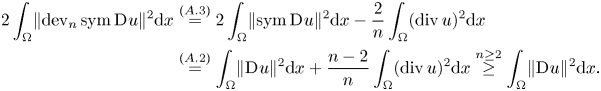 \begin{align*} 2 \int_\Omega \lVert{\operatorname{dev}_n\operatorname{sym} \operatorname{D}\hspace{-1pt} u}\rVert^{2}\mathrm{d}{x}&\overset{(A.3)}{=} 2 \int_\Omega \lVert{\operatorname{sym} \operatorname{D}\hspace{-1pt} u}\rVert^{2}\mathrm{d}{x} -\frac 2n\int_\Omega(\operatorname{div} u)^{2}\mathrm{d}{x}\\ &\overset{(A.2)}{=} \int_\Omega \lVert{\operatorname{D}\hspace{-1pt} u}\rVert^{2}\mathrm{d}{x} +\frac{n-2}{n}\int_\Omega(\operatorname{div} u)^{2}\mathrm{d}{x}\overset{n\ge 2}{\ge}\int_\Omega \lVert{\operatorname{D}\hspace{-1pt} u}\rVert^{2}\mathrm{d}{x}.\end{align*}
□
Remark 31 The trace-free Korn's first inequality (A.1) is also valid in  $L^{p}$,
  $p>1$, see [Reference Fuchs and Schirra27, Prop. 1] for the
  $n=2$ case and [Reference Schirra65, Thm. 2.3] for all
  $n\geq 2$ where again the justification was based on the Lions lemma.
Appendix A.2 Infinitesimal planar conformal mappings
Infinitesimal conformal mappings are defined by  $\operatorname {dev}_n\operatorname {sym}\operatorname {D}\hspace {-1pt} u \equiv 0$ and in
  $n>2$ they have the representation
 \[ \big\langle{a},{x}\big\rangle\,x-\frac 12a\lVert{x}\rVert^{2}+A\,x +\beta\,x +c, \quad \text{with }A\in\mathfrak{so}(n), a,c\in\mathbb{R}^{n} \text{ and }\beta\in\mathbb{R}, \]
cf. [Reference Dain17, Reference Jeong and Neff33, Reference Neff, Jeong and Ramezani49, Reference Reshetnyak63–Reference Schirra65].
In the planar case, the situation is quite different. Indeed, the condition  $\operatorname {dev}_2\operatorname {sym} \operatorname {D}\hspace {-1pt} u \equiv 0$ reads
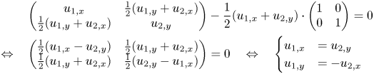 \begin{align*} &\begin{pmatrix} u_{1,x} & \frac 12(u_{1,y}+u_{2,x}) \\ \frac 12(u_{1,y}+u_{2,x}) & u_{2,y} \end{pmatrix}- \frac 12(u_{1,x}+u_{2,y})\cdot \begin{pmatrix} 1 & 0\\ 0 & 1\end{pmatrix} = 0 \\ \Leftrightarrow \quad & \begin{pmatrix} \frac 12(u_{1,x}-u_{2,y}) & \frac 12(u_{1,y}+u_{2,x}) \\ \frac 12(u_{1,y}+u_{2,x}) & \frac 12(u_{2,y}-u_{1,x}) \end{pmatrix}= 0 \quad \Leftrightarrow \quad \begin{cases} u_{1,x} & =u_{2,y} \\ u_{1,y} & ={-}u_{2,x} \end{cases} \end{align*}
and corresponds to the validity of the Cauchy-Riemann-equations. Thus, in the planar case, infinitesimal conformal mappings are conformal mappings.
Appendix A.3 Kröner's relation in infinitesimal elasto-plasticity
At the macroscopic scale, in infinitesimal elasto-plastic theory, see e.g. [Reference Amstutz and Van Goethem3, Reference Amstutz and Van Goethem4, Reference Ebobisse and Neff20–Reference Ebobisse, Neff and Forest22, Reference Li44, Reference Maggiani, Scala and Van Goethem46], the incompatibility of the elastic strain is related to the  $\operatorname {Curl}$ of the contortion tensor
  $\kappa : = \alpha ^{T} -\frac 12\operatorname {tr}(\alpha )\cdot {\mathbb{1}}$, where
  $\alpha : = \operatorname {Curl} P$ is the dislocation density tensor, by Kröner's relation [Reference Kröner35]:
 \begin{equation} \boldsymbol{\operatorname{inc}}\,(\operatorname{sym} e) ={-}\operatorname{Curl} \kappa, \end{equation}
where the additive decomposition of the displacement gradient into non-symmetric elastic and plastic distortions is assumed:
 \begin{equation} \operatorname{D}\hspace{-1pt} u = e + P. \end{equation}
Indeed, (A.4) follows from Nye's formula (2.16) and the identities
 \[ \operatorname{tr}\operatorname{Curl}\operatorname{sym} e = 0 \quad \text{as well as} \quad \alpha: = \operatorname{Curl} P\overset{(A.5)}{=}-\operatorname{Curl} e, \]
since we have
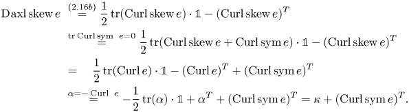 \begin{align} \operatorname{D}\hspace{-1pt} \operatorname{axl} \operatorname{skew} e \ &\overset{(2.16b)}{=}\frac 12\operatorname{tr}(\operatorname{Curl}\operatorname{skew} e)\cdot{\mathbb{1}}-(\operatorname{Curl}\operatorname{skew} e)^{T}\nonumber\\
& \overset{\operatorname{tr}\operatorname{Curl}\operatorname{sym}\ e = 0}{=}\frac 12\operatorname{tr}(\operatorname{Curl}\operatorname{skew} e+\operatorname{Curl}\operatorname{sym} e)\cdot{\mathbb{1}}-(\operatorname{Curl}\operatorname{skew} e)^{T}\nonumber\\
&=\quad \frac 12\operatorname{tr}(\operatorname{Curl} e)\cdot{\mathbb{1}}-(\operatorname{Curl} e)^{T}+ (\operatorname{Curl}\operatorname{sym} e)^{T}\nonumber\\
&\overset{\alpha={-}\operatorname{Curl}\ e}{=} -\frac 12\operatorname{tr}(\alpha)\cdot{\mathbb{1}} + \alpha^{T} + (\operatorname{Curl}\operatorname{sym} e)^{T} = \kappa + (\operatorname{Curl}\operatorname{sym} e)^{T}. \end{align}
\begin{align} \operatorname{D}\hspace{-1pt} \operatorname{axl} \operatorname{skew} e \ &\overset{(2.16b)}{=}\frac 12\operatorname{tr}(\operatorname{Curl}\operatorname{skew} e)\cdot{\mathbb{1}}-(\operatorname{Curl}\operatorname{skew} e)^{T}\nonumber\\
& \overset{\operatorname{tr}\operatorname{Curl}\operatorname{sym}\ e = 0}{=}\frac 12\operatorname{tr}(\operatorname{Curl}\operatorname{skew} e+\operatorname{Curl}\operatorname{sym} e)\cdot{\mathbb{1}}-(\operatorname{Curl}\operatorname{skew} e)^{T}\nonumber\\
&=\quad \frac 12\operatorname{tr}(\operatorname{Curl} e)\cdot{\mathbb{1}}-(\operatorname{Curl} e)^{T}+ (\operatorname{Curl}\operatorname{sym} e)^{T}\nonumber\\
&\overset{\alpha={-}\operatorname{Curl}\ e}{=} -\frac 12\operatorname{tr}(\alpha)\cdot{\mathbb{1}} + \alpha^{T} + (\operatorname{Curl}\operatorname{sym} e)^{T} = \kappa + (\operatorname{Curl}\operatorname{sym} e)^{T}. \end{align}
Thus, applying  $\operatorname {Curl}$ on both sides of (A.6) establishes (A.4), since
  $\operatorname {Curl}\circ \operatorname {D}\hspace {-1pt} \equiv 0$:
 \begin{align} 0 = \operatorname{Curl} \operatorname{D}\hspace{-1pt}\operatorname{axl} \operatorname{skew} e \overset{(A.6)}{=} \operatorname{Curl} \kappa +\operatorname{Curl}([\operatorname{Curl}\operatorname{sym} e]^{T})= \operatorname{Curl} \kappa + \boldsymbol{\operatorname{inc}}\, (\operatorname{sym} e). \end{align}
From the decomposition  $\operatorname {sym} \operatorname {D}\hspace {-1pt} u = \operatorname {sym} e + \operatorname {sym} P$ it follows moreover
  $\boldsymbol {\operatorname {inc}}\,(\operatorname {sym} e) = -\boldsymbol {\operatorname {inc}}\,(\operatorname {sym} P)$, see also the last calculation in footnote 5.
In finite strain elasticity [Reference Ciarlet10], the Riemann-Christoffel tensor  $\mathcal {R}$ expresses the compatibility of strain tensors in the sense of
 \begin{align} & C \in C^{2}(\Omega, \operatorname{Sym}^{+}(3)): \quad \mathcal{R}(C)= 0 \quad \Leftrightarrow\notag\\ &C = (D\varphi)^{T} D\varphi \quad \text{in simply connected domains}.\end{align}
Writing  $C=({\mathbb{1}}+P)^{T}({\mathbb{1}} +P)= 1 + 2 {\cdot }\operatorname {sym} P + P^{T}P$ for
 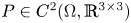 $P \in C^{2}(\Omega ,\mathbb {R}^{3\times 3})$, the incompatibility operator is the linearization of the Riemann-Christoffel tensor at the identity, since
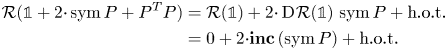 \begin{align}
\mathcal{R}({\mathbb{1}} + 2
{\cdot}\operatorname{sym} P + P^{T}P) &=
\mathcal{R}({\mathbb{1}})+2
{\cdot}\operatorname{D}\hspace{-1pt}
\mathcal{R}({\mathbb{1}})\,\operatorname{sym}
P + \text{h.o.t.}\notag\\
& = 0 + 2
{\cdot}\boldsymbol{\operatorname{inc}}\,(\operatorname{sym}
P) + \text{h.o.t.}
\end{align}
\begin{align}
\mathcal{R}({\mathbb{1}} + 2
{\cdot}\operatorname{sym} P + P^{T}P) &=
\mathcal{R}({\mathbb{1}})+2
{\cdot}\operatorname{D}\hspace{-1pt}
\mathcal{R}({\mathbb{1}})\,\operatorname{sym}
P + \text{h.o.t.}\notag\\
& = 0 + 2
{\cdot}\boldsymbol{\operatorname{inc}}\,(\operatorname{sym}
P) + \text{h.o.t.}
\end{align}see also [Reference Ebobisse and Neff20] and the references contained therein.
Appendix A.4 Further identities
Symmetric tensors play an important role in the above considerations. We mention here the full expression of  $S\times b$ for
  $S\in \operatorname {Sym}(3)$ and
  $b\in \mathbb {R}^{3}$:
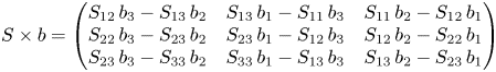 \begin{equation} S \times b = \begin{pmatrix} S_{12}\,b_3 - S_{13}\,b_2 & S_{13}\, b_1 - S_{11}\,b_3 & S_{11}\,b_2 - S_{12}\,b_1\\ S_{22}\,b_3 - S_{23}\,b_2 & S_{23}\, b_1 - S_{12}\,b_3 & S_{12}\,b_2 - S_{22}\,b_1\\ S_{23}\,b_3 - S_{33}\,b_2 & S_{33}\, b_1 - S_{13}\,b_3 & S_{13}\,b_2 - S_{23}\,b_1 \end{pmatrix} \end{equation}
which is an example of a trace-free matrix with non-zero entries on the diagonal:
 \[ \operatorname{tr}(S \times b) = S_{12}\,b_3 - S_{13}\,b_2 + S_{23}\, b_1 - S_{12}\,b_3 + S_{13}\,b_2 - S_{23}\,b_1 = 0. \]
Moreover, we outline some basic identities which played useful roles in our considerations:
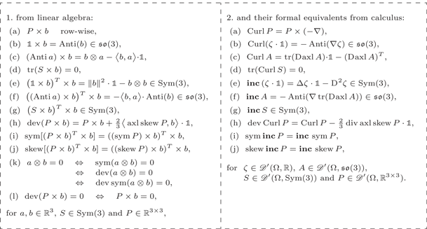
We catch up with the verification of the identities not contained in our considerations explicitly:
•
$({\mathbb{1}}\,{\times}\, b)^{T}\,{\times}\, b \overset {\text {1.(a)}}{=}(\operatorname {Anti}(b))^{T}\times b = -(\operatorname {Anti} b)\times b \overset {\text {1.(b)}}{=} - b\otimes b +\langle {b},{b}\rangle {\cdot }{\mathbb{1}} \ \Rightarrow \ \text {1.(d)}$,• we have the decompositions:
but also\begin{align*} (P\times
b)^{T}\times b &= (\operatorname{sym} P \times b +
\operatorname{skew} P\times b)^{T} \times b\notag\\
& =
\underset{\in\operatorname{Sym}(3)}{\underbrace{((\operatorname{sym}
P)\times b)^{T}\times b}} +
\underset{\in\mathfrak{so}(3)}{\underbrace{((\operatorname{skew}
P)\times b)^{T}\times b}} \end{align*}
where we have used (e) and (f), so that (h) and (i) follow,\[ \boldsymbol{\operatorname{inc}}\, P = \boldsymbol{\operatorname{inc}}\,(\operatorname{sym} P + \operatorname{skew} P) = \underset{\in\operatorname{Sym}(3)}{\underbrace{\boldsymbol{\operatorname{inc}}\,\operatorname{sym} P}} + \underset{\in\mathfrak{so}(3)}{\underbrace{\boldsymbol{\operatorname{inc}}\, \operatorname{skew} P}} \]
• the equivalence
$a\otimes b = 0$ $\Leftrightarrow$ $\operatorname {dev}\operatorname {sym}(a\otimes b)=0$ follows from the expression:
\[ \frac{\lVert{b}\rVert^{4}}{2}\lVert{a\otimes b}\rVert^{2} = \lVert{b}\rVert^{4}\lVert{\operatorname{dev}\operatorname{sym}(a\otimes b)}\rVert^{2}+\frac 12\left(\frac{n}{n-1}\right)^{2}\big\langle{b},{\operatorname{dev}\operatorname{sym}(a\otimes b) b}\big\rangle^{2}. \]

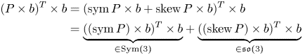
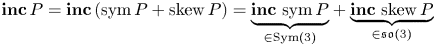


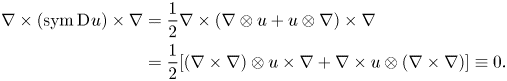


 Open access