1. INTRODUCTION
Receiver Autonomous Integrity Monitoring (RAIM) is an integrity monitoring method in which an airborne receiver performs self-contained fault detection (Lee, Reference Lee1986; Parkinson and Axelrad, Reference Parkinson and Axelrad1988; Sturza, Reference Sturza1988; Brown, Reference Brown1992). Several RAIM algorithms have been considered in the literature (Lee, Reference Lee1986; Brown, Reference Brown1992; Angus, Reference Angus2006; Ene et al., Reference Ene, Blanch and Powell2007; Schroth et al., Reference Schroth, Rippl, Ene, Blanch, Belabbas, Walter, Enge and Meurer2008; Blanch et al., Reference Blanch, Walter and Enge2010; Wu et al., Reference Wu, Wang and Jiang2013). When utilising the Global Positioning System (GPS) as a navigational means in aviation, RAIM is only required to consider the occurrence of a single satellite failure. This is due to the probability of two simultaneous satellite failures at a particular location being estimated as 1 × 10⁻⁸, which is significantly smaller than the 1 × 10⁻⁷ probability required (Pervan et al., Reference Pervan, Pullen and Christie1998; Ober, Reference Ober2003; Lee, Reference Lee2004; Knight et al., Reference Knight, Wang, Rizos and Han2009; Knight and Wang, Reference Knight and Wang2009). However, along with the revitalisation of the Globalnaya Navigatsionnaya Sputnikovaya Sistema (GLONASS) system and the current development of Galileo and Beidou (BDS) systems, the availability of RAIM algorithms is greatly increased in an integrated navigation system. However, the probability of a user experiencing multiple failures simultaneously will be too high to ignore (Knight et al., Reference Knight, Wang, Rizos and Han2009).
In recent years, a few approaches have been considered in the literature for handling multiple satellite faults. Angus (Reference Angus2006) focused on providing an exact solution to the problem of extending RAIM protection levels for single fault to the case of protecting for multiple faults. Knight et al. (Reference Knight, Wang, Rizos and Han2009) designed a RAIM algorithm for removing two satellite faults by extending the χ2 test statistics. Hewitson and Wang (Reference Hewitson and Wang2006) pointed out that an extended w-test identification procedure can be used for the simultaneous removal of multiple outliers simply and effectively, provided the navigation adjustment is sufficiently resilient to the contaminating measurements. Wang and Wang (Reference Wang and Wang2007) introduced robust M-estimation schemes into a RAIM algorithm, and demonstrated that the M-estimation can mitigate the effect of multiple satellite faults in the Global Navigation Satellite System (GNSS) navigation solution. In fact, any robust method can serve this purpose, such as least median of squares (Rousseuw, Reference Rousseeuw1984) and sign-constrained robust least squares (Xu, Reference Xu2005). However, quick and robust methods are demanding in real time applications. Schroth et al. (Reference Schroth, Rippl, Ene, Blanch, Belabbas, Walter, Enge and Meurer2008) proposed a Range Consensus (RANCO) RAIM algorithm for dealing with multiple satellite faults. The main idea of RANCO is that it calculates the position solutions based on subsets of four satellites and compares the estimate with the pseudoranges of all the satellites not contributing to this solution. Ene et al. (Reference Ene, Blanch and Powell2007) discussed a multiple hypothesis solution separation (MHSS) RAIM algorithm to treat multiple satellite faults.
It is noticeable that although these methods above can solve problems in the corresponding practical fields, they have several disadvantages (Angus, Reference Angus2006; Hewiston and Wang, Reference Hewitson and Wang2006; Schroth et al., Reference Schroth, Rippl, Ene, Blanch, Belabbas, Walter, Enge and Meurer2008). Firstly, the current non-Bayesian methods are based on classical hypothesis testing and the threshold for fault detection often depends on the measured noise and false alarm probability. For instance, the probability of correctly detecting faults by the RANCO method is affected by the threshold. Secondly, most of the current RAIM algorithms, such as the RANCO method, use the measurement domain rather than the position domain. However, the probability of missed detection of the measurement domain is often defined as the probability of an undetected measurement bias rather than that of the unallowable position error (Ober, Reference Ober2003). In the position domain methods, a failure is detected as soon as the accuracy or integrity requirements are not met. Thirdly, the traditional RAIM algorithms do not consider the historical observations of satellite and receiver. Fourthly, the exact probabilities of hazardously misleading information are not given and then the availability of the navigation system is either underestimated or overestimated. Fortunately, Bayesian methods can exactly compute the probabilities of hazardously misleading information in the problem of integrity monitoring (cf. Ober, Reference Ober2000).
In fact, the Bayesian RAIM methods for handling a single satellite fault have been developed to a certain extent. Ober (Reference Ober2000) pointed out that the positioning performance can be described as a weighted sum of error distributions in which the weights depend on the measurement residuals, the statistical properties of the measurements and a prior probability of fault. Further, the weights could be used as a testing statistic to detect faults. Pesonen (Reference Pesonen2009) proposed a RAIM method using Bayesian statistical decision theory, but the method depends on a user-defined loss function to model the relative costs of false alarms and missed detection. Pesonen and Piché (Reference Pesonen and Piché2009) designed a RAIM algorithm based on Bayesian model comparison theory. However, when the posterior probability odds are near the critical values, the results are not reliable. Pesonen (Reference Pesonen2011) analysed the RAIM performance parameters of accuracy, availability, continuity and integrity from the viewpoint of Bayesian statistics and pointed out that in the Bayesian framework all of the problems of faults detection, identification and integrity could be converted into a computation concerning the posterior probability distributions of the positioning parameters, but an effective computation algorithm is not given in that paper. None of the Bayesian RAIM methods above can deal with multiple satellite faults.
Therefore, a new Bayesian RAIM approach for multiple satellite fault detection and exclusion is proposed based on the classification variables in this article. The paper is organised as follows. Section 2 introduces a classification variable to each satellite observation; a rule for multiple satellite fault detection and exclusion is proposed based on the posterior probabilities of the classification variables in the respective of Bayesian hypothesis testing. In Section 3, the Gibbs sampler is introduced to solve the computing problem of the posterior probabilities of the classification variables. Therefore, the posterior distributions that are needed by the Gibbs sampler are deduced. In Section 4, the implementation of the Bayesian RAIM algorithm is designed with the Gibbs sampler and a flow chart is given. In Section 5, designs of several experiments to evaluate the effectiveness of the proposed Bayesian RAIM algorithm in the case of multiple faults are given. Real observations of the CHAN station of the International GNSS Service (IGS) are analysed by this algorithm. In Section 6, conclusions are summarised.
2. MULTIPLE FAULTS DETECTION AND EXCLUSION BASED ON CLASSIFICATION VARIABLES
2.1. Model and rule
It is assumed that n denotes the number of visible satellites and the system of the linearized GNSS equation of the pseudo-range observations is as follows:
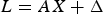 $$L = AX + \Delta $$
Where L = (L 1, … , L n)T is the n × 1 vector of observations containing the differences between the expected ranging values and the raw pseudo-range observations to each of the n satellites; A = (a 1, … , a n)T is the n × 4 observation matrix; X is the 4 × 1 vector of parameters which contain the three components of the true position deviation from the nominal position and the user clock bias deviation; Δ = (Δ1, … , Δn)T is the n × 1 vector of measurement errors where Δi contains the clock/ephemeris error, the residual tropospheric errors, the residual ionospheric errors, receiver noise and multipath error. It is assumed that Δ~N n (0, σ 02P− 1), where  $\sigma _0^2 $ is an unknown variance of unit weight and P = diag (p 1, … , p n) is a known weight matrix. Let
  $\tau = \sigma _0^{ - 2} $.
In this paper, the problem of satellite fault detection and exclusion is converted into the problem of outlier detection and identification (cf. Wang and Wang, Reference Wang and Wang2007). Since outlier detection is done explicitly in the position domain, we do not use the conventional mean-shift model (Koch, Reference Koch.1999; Gui et al., Reference Gui, Li, Gong, Li and Li2011) for fault detection. Instead, we assume that when the observation L i does not contain an outlier, the corresponding error Δi ~ N(0, τ− 1p i−1); otherwise the error Δi has the variance-inflation normal distribution (Koch, Reference Koch.1999), that is to say, Δi~N(0, k 2τ− 1p i−1) where k > 1 is called an inflation coefficient.
A classification variable δ i is introduced for each observation L i to detect outliers, which is defined as
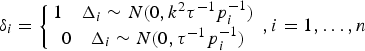 $$\delta _i = \left\{ \matrix{1\quad \Delta _i \sim N(0, k^2 \tau _{}^{ - 1} p_i^{ - 1} ) \cr 0\quad \Delta _i \sim N(0, \tau _{}^{ - 1} p_i^{ - 1} ) } \right.,i = 1, \ldots, n$$
That is to say, when the classification variable δ i equals 0, it denotes that L i is normal; otherwise when the classification variable δ i equals 1, it denotes that L i contains an outlier.
Thus, the model for satellite faults detection and exclusion can be reformulated as follows:
 $$\left\{ \matrix{L = AX + \Delta \cr \Delta _i \sim (1 - \delta _i )N(0, \tau _{}^{ - 1} p_i^{ - 1} ) + \delta _i N(0, k^2 \tau _{}^{ - 1} p_i^{ - 1} ),i = 1, \ldots, n } \right.$$
We allow for a small prior probability α that any given observation is affected by an outlier, where α << 1 − α, which means that the observation is assumed to be normal according to the prior information. Then the prior odds ratio for δ i = 1 to δ i = 0 is
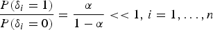 $$\displaystyle{{P(\delta _i = 1)} \over {P(\delta _i = 0)}} = \displaystyle{\alpha \over {1 - \alpha}} \lt \lt 1,\,i = 1, \ldots, n$$
After we obtain the observation vector L, the posterior odds ratio for δ i = 1 to δ i = 0 is given by
 $$\displaystyle{{P(\delta _i = 1\vert L)} \over {P(\delta _i = 0\vert L)}} = \displaystyle{\alpha \over {1 - \alpha}} \times {\rm observation\,information,}\,i = 1, \ldots, n$$
According to the principle of Bayesian hypothesis testing (Berger, Reference Berger1985; Koch, Reference Koch2007), when 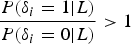 $\displaystyle{{P(\delta _i = 1\vert L)} \over {P(\delta _i = 0\vert L)}} \gt 1$, we identify that L i contains an outlier; otherwise, L i is normal. Since P(δ i = 1|L) + P(δ i = 0|L)=1,
  $\displaystyle{{P(\delta _i = 1\vert L)} \over {P(\delta _i = 0\vert L)}} \gt 1$ is equivalent to
 $$P(\delta _i = 1\vert L) \gt 0.5$$
In conclusion, a rule of detecting multiple outliers based on the posterior probabilities of the classification variables is proposed as follows. When we obtain the observation vector L, the posterior probability of each observation L i containing an outlier is computed, q i = P(δ i = 1|L), i = 1, …, n. If q i>0·5, we identify that L i contains an outlier.
2.2. Prior distributions of the unknown parameters
To follow the principle of Bayesian statistics, the prior distributions of the parameters X, τ and δ ii = 1, …, n which are considered to be random variables are assigned as follows.
Firstly, according to the definition of the classification variables, the prior distribution of δ i can be modelled by the two point distribution:
 $$\delta _i \sim b(1,\alpha ),i = 1, \ldots, n$$
If we do not know anything about the unknown parameters X and τ, we can model them by a non-informative prior density function according to Fisher's information matrix (Koch, Reference Koch2007), that is to say,
 $$p(X,\tau ) \propto \displaystyle{1 \over \tau} $$
If there is available historical information about the unknown parameters X and τ, we can model them by the conjugate principle (Berger, Reference Berger1985; Koch, Reference Koch2007), that is to say, the prior distribution of X and τ has the normal-gamma distribution (X,τ) ~ NG(X 0,τ− 1Σ0−1,α 0,α 1) with the hyper parameters X 0, Σ0, α 0 and α 1, which are determined by the historical data.
3. COMPUTATION OF THE POSTERIOR PROBABILITIES BASED ON THE GIBBS SAMPLER
According to Section 2, the problem of satellite fault detection and exclusion is converted into the computation problem of the posterior probabilities of the corresponding classification variables. Since the distributions involved by the posterior probabilities q i = P(δ i = 1|L), i = 1,…, n are complex, we use a Gibbs sampler (Ethier and Kurtz, Reference Ethier and Kurtz1986; Koch, Reference Koch2007; Gui et al., Reference Gui, Li, Gong, Li and Li2011) to solve the computation problem. Let δ = (δ 1, … , δ n) and δ (−i) = (δ 1, … , δ i−1,δ i+1, … , δ n), i = 1, … , n.
Firstly, in order to compute P(δ i = 1|L), i = 1, … , n by the Gibbs sampler, we deduce the posterior distributions of the parameters X, τ and δ ii = 1, … , n.
When the prior distribution of the unknown parameters X and τ has the normal-gamma distribution (X,τ) ~ NG (X 0,τ− 1Σ0−1,α 0,α 1), we can obtain the posterior distribution of X, τ and δ ii = 1, … ,n according to Bayes' theorem (Berger, Reference Berger1985; Koch, Reference Koch2007),
 $$\left\{ {X\left\vert {\tau, \delta, L} \right.} \right\}\sim N_t (\tilde X,\tau ^{ - 1} \Sigma _1 ^{ - 1} )$$
 $$\left\{ {\tau \left\vert {X,\delta, L} \right.} \right\}\sim \Gamma (\alpha _2, \alpha _3 )$$
 $$\left\{ {\delta _i \left\vert {X,\tau, \delta _{( - i)}, L} \right.} \right\}\sim b(1,\tilde q_i^{} ),\,i = 1, \ldots, n$$
where
 $$\tilde X = (A^T \tilde PA + \Sigma _0 )^{ - 1} (A^T \tilde PL + \Sigma _0 X_0 )$$
 $$\Sigma _1 = A^T \tilde PA + \Sigma _0 $$
 $$\alpha _2 = \displaystyle{{n + t + 2\alpha _0} \over 2}$$
 $$\alpha _3 = \displaystyle{{(L - AX)^T \tilde P(L - AX) + (X - X_0 )^T \Sigma _0 (X - X_0 ) + 2\alpha _1} \over 2}$$
 $$\tilde P = {\rm diag}\left(\displaystyle{{\,p_1} \over {1 + \delta _1 (k^2 - 1)}}, \ldots, \displaystyle{{\,p_n} \over {1 + \delta _n (k^2 - 1)}}\right)$$
 $$\eqalign{&\tilde{q}_i = P(\delta_i = 1 \left\vert X, \tau, \delta _{( - i)}, L \right.) = \displaystyle{\alpha \varphi (\Delta_i \sqrt{p_i \tau} / k) \over \alpha \varphi (\Delta _i \sqrt{p_i \tau} / k) + k(1 - \alpha) \varphi (\Delta _i \sqrt{p_i \tau})}, i = 1, \ldots, n \cr &\qquad \Delta_i = L_i - a_i^T X, i = 1, \ldots, n}$$
and φ(·) denotes the probability density function of the normal distribution. The derivation of Equation (17) is given in the Appendix.
In particular, when we assume a non-informative prior density function for the unknown parameters X and τ, the corresponding hyper parameters included in the posterior distribution of X, τ and δ ii = 1, … ,n are given by
 $$\tilde X = (A^T \tilde PA)^{ - 1} A^T \tilde PL$$
 $$\Sigma _1 = A^T \tilde PA$$
 $$\alpha _2 = \displaystyle{n \over 2}$$
 $$\alpha _3 = \displaystyle{{(L - AX)^T \tilde P(L - AX)} \over 2}$$
Secondly, the approximate formula for computing P(δ i = 1|L) is deduced in the following Section. In fact, we can obtain
 $$\eqalign{q_i = & P(\delta _i = 1\vert L) = \int\!\int\!\int {P(} \delta _i = 1,X,\tau, \delta _{( - i)} \vert L)dXd\tau d\delta _{( - i)} \cr = & \int\!\int\!\int P (\delta _i = 1\vert X,\tau, \delta _{( - i)}, L)p(X,\tau, \delta _{( - i)} \vert L)dXd\tau d\delta _{( - i)} \cr = & E_{X,\tau, \delta _{( - i)} \vert L} \{ P(\delta _i = 1\vert X,\tau, \delta _{\left( { - i} \right)}, L)\}, i = 1, \ldots, n} $$
It is assumed that {X (s),τ (s),δ (s),s = 1, … , R} is a set of stationary random samples that are drawn iteratively from the posterior distributions Equations (9) to (11) by the Gibbs sampler. Combining Equation (22) with Equation (17), we can obtain a formula for computing the posterior probabilities of the classification variables,
 $$\eqalign{& \hat q_i \approx \displaystyle{1 \over R}\sum\limits_{s = 1}^R {\displaystyle{{\alpha \varphi (k^{ - 1} (L_i - a_i^T X^{(s)} )\sqrt {\,p_i^{(s)} \tau _{}^{(s)}} )} \over {\alpha \varphi (k^{ - 1} (L_i - a_i^T X^{(s)} )\sqrt {\,p_i^{(s)} \tau _{}^{(s)}} ) + k^{} (1 - \alpha )\varphi ((L_i - a_i^T X^{(s)} )\sqrt {\,p_i^{(s)} \tau _{}^{(s)}} )}}} \cr & \quad \quad \quad \quad \quad \quad \quad \quad \quad \quad \quad \quad \quad \quad \quad \quad \quad \quad \quad \quad i = 1, \ldots, n} $$
4. IMPLEMENTION FOR MULTIPLE FAULTS DETECTION AND EXCLUSION BASED ON BAYESIAN METHODS
A new Bayesian RAIM algorithm is designed for multiple faults detection and exclusion by the Gibbs sampler.
Step 1. Choose the initial conditions y (0) = (X (0),τ (0),δ (0)) of the Gibbs sampler where each element of δ (0) is equal to 1 with a probability of α.
If we use a non-informative prior density function for X and τ, the initial value X (0) is assigned as 0 and τ (0) equals to $\displaystyle{1 \over {(\sigma _0^2 )^{(0)}}} $, where the initial value (σ 02)(0) is determined by the range errors.
If the prior distribution of X andτ has a normal-gamma distribution (X,τ) ~ NG (X 0, τ− 1Σ0−1, α 0, α 1), the initial value X (0) is determined by X (0) = (ATP (0)A + Σ0)−1 (ATP (0)L + Σ0X 0), where the weight 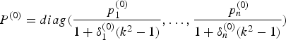 $P^{(0)} = diag (\displaystyle{{\,p_1^{(0)}} \over {1 + \delta _1^{(0)} (k^2 - 1)}}, \ldots, \displaystyle{{\,p_n^{(0)}} \over {1 + \delta _n^{(0)} (k^2 - 1)}})$ is determined by the ratios of
 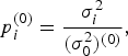 $p_i^{(0)} = \displaystyle{{\sigma _i^2} \over {(\sigma _0^2 )^{(0)}}}, $ and X 0, Σ0 are estimated empirically. The variance
  $\sigma _i^2 $ of measurement noise is given by the formula
  $\sigma _i^2 = \sigma _{_{URA}} ^2 + \sigma _{tro,i}^2 + \sigma _{ion,i}^2 + \sigma _{SNR,i}^2 + \sigma _m^2, $ where
  $\sigma _{_{URA}} ^2 $ is the variance of the clock/ephemeris error,
  $\sigma _{tro,i}^2 $ is the variance of the residual tropospheric error,
  $\sigma _{ion,i}^2 $ is the variance of the residual ionosphere error,
  $\sigma _{SNR,i}^2 $ is the variance of receiver noise and
  $\sigma _m^2 $ is the variance of multipath. The initial value τ (0) is obtained by sampling from the posterior distribution p(τ|L,δ (0), X (0)) = Γ
  $(\alpha _2^{(0)}, \alpha _3^{(0)} )$, where
 $$\alpha _2^{(0)} = \displaystyle{{n + t + 2\alpha _0} \over 2}$$
 $$\alpha _3^{(0)} = \displaystyle{{(L - AX^{(0)} )^T P^{(0)} (L - AX^{(0)} ) + (X^{(0)} - X_0 )^T \Sigma _0 (X^{(0)} - X_0 ) + 2\alpha _1} \over 2}$$
and α 0, α 1 are determined empirically.
Also, the reasonable inflation coefficient k in the model Equation (3) is chosen as 3–5 according to the 3σ principle of normal distribution.
Step 2. Implement the standard Gibbs sampler. Suppose that the (s-1)th realisation is (X (s−1), τ (s−1), δ (s−1)). Then the sth realisation can be obtained as follows:
 $$\eqalign{ & X^{\left( s \right)}\ {\rm is\,drawn\,from}\, p\,(X\vert \tau ^{\left( {s - 1} \right)}, \delta ^{\left( {s - 1} \right)}, L), \cr & \tau ^{(s)}\ {\rm is\,drawn\,from}\,p\,(\tau \left\vert {L,\delta ^{(s - 1)}, X^{(s)}} \right.), \cr & \delta _i ^{\left( s \right)}\ {\rm is\,drawn\,from}\,p\,(\delta _i \vert X^{\left( s \right)}, \tau ^{\left( s \right)}, \delta _1^{\left( s \right)}, \ldots, \delta _{i - 1}^{\left( s \right)}, \delta _{i + 1}^{\left( {s - 1} \right)}, \ldots, \delta _n^{\left( {s - 1} \right)}, L),\,i = 1, \ldots, n} $$
 Run the Gibbs sampler until it is stationary where the judging criteria for the stationary Gibbs sampler in this paper are as follows: if 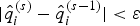 $\vert \hat q_i^{(s)} - \hat q_i^{(s - 1)} \vert \lt \varepsilon $, then we claim that the Gibbs sampler is stationary, where ε is a given constant that is sufficiently small. Then, a set of samples (X (1),τ (1),δ (1)), … ,(X (R),τ (R),δ (R)) can be obtained.
Step 3. Compute the posterior probabilities of the classification variables by Equation (23) and detect outliers by the rule proposed in Section 2.1.
The detailed flow chart of the Bayesian RAIM algorithm is shown at Figure 1.

Figure 1. Flow chart of the Bayesian RAIM algorithm.
5. EXAMPLES AND ANALYSIS
5.1. Example 1
To illustrate the effects of the proposed algorithm for detecting and excluding multiple satellite faults, we simulate the pseudo-range observations of an integrated GPS/BDS constellation using Satellite Toolkit (STK). The data were collected from 00:10:01 of 15 January 2013 to 00:10:01 of 16 January 2013, with the selected site in Zhengzhou (Lat 34·6836°N, Lon 113·533°E, Altitude: 0·0 m). The sampling rate was 30 s.
The observations are single frequency pseudo-range measurements, including the errors of clock/ephemeris, residual tropospheric, residual ionosphere, receiver noise and multipath whose standard deviations are given by
 $$\sigma _{URA}^{} = \sigma _0 = 1\,{\rm m},\,\sigma _{tro,i}^{} = 0.5\,{\rm m},\,\sigma _{ion,i}^{} = 5\,{\rm m},\,\sigma _{SNR,i}^{} = 0.2\,{\rm m},\,\sigma _m^{} = 1\,{\rm m}$$
respectively.
The number of visible satellites, the GDOP values and the simulated sky plot of the integrated GPS/BDS constellation are shown in Figures 2 and 3, respectively.
Figure 2. The numbers of visible satellites and the GDOP values of Zhengzhou station.
Figure 3. The sky plot of the simulated integrated GPS/BDS constellation.
We assign a normal-gamma distribution as prior for X and τ. And the inflation coefficient k in the model Equation (3) is chosen as 3.
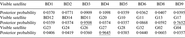
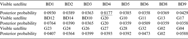
The experimental schemes are designed as follows. Firstly, we introduce three faults with the sizes 60 m, 25 m and 45 m in BD11, G17 and G27 respectively at epoch 150. Secondly, we introduce two faults with the sizes 65 m and 30 m in BD4 and G20 respectively at epoch 500.
The posterior probabilities of the classification variables corresponding to the pseudo-range observations at epoch 150 and 500 are shown in Tables 1 and 2, respectively. The position errors before and after the faults exclusion are shown in Figures 4 and 5, respectively.
Figure 4. Position errors before faults exclusion.
Figure 5. Position errors after faults exclusion.
Table 1. The posterior probabilities of the classification variables corresponding to the pseudorange observations at epoch 150.
Table 2. The posterior probabilities of the classification variables corresponding to the pseudorange observations at epoch 500.
From Table 1, we can see that the posterior probabilities of the classification variables corresponding to the pseudo-range observations of BD11, G17 and G27 at epoch 150 are larger than 0·5, which shows that the three faults at epoch 150 are successfully detected by the proposed method.
From Table 2, it can be seen that the posterior probabilities of the classification variables corresponding to the pseudo-range observations of BD4 and G20 at epoch 500 are larger than 0·5. This means that the two faults at epoch 500 are also successfully detected.
Comparing Figure 4 with Figure 5 we can see that the position errors at epoch 150 and 500 are decreased after faults exclusion.
5.2. Example 2
To check the probability of correctly detecting faults of the proposed Bayesian RAIM algorithm, we compare the method in this paper with the RANCO method that is proposed by Stanford University (Schroth et al., Reference Schroth, Rippl, Ene, Blanch, Belabbas, Walter, Enge and Meurer2008).
We simulate the pseudo-range observations of an integrated GPS/BDS constellation to implement our experiment. The sampling rate is 30 s. The simulated sites are spread worldwide with 24 user points that are retrieved from GPS Minimum Operational Performance Standards (MOPS) from the Radio Technical Commission for Aeronautics (RTCA). We randomly select 3–6 satellites at each user point and introduce range biases to the selected satellites, where the range biases are increased from 5 m to 145 m with a step length of 5 m. The experiment duration is equivalent to 6599 epochs.
We assign a non-informative distribution prior for X and τ. The inflation coefficient k in the model Equation (3) is chosen as 3.
The observations are single frequency pseudo-range measurements where the simulated errors are the same as that in Example 5·1. Figure 6 shows the probability of correctly detecting faults of the Bayesian method and the RANCO method.
Figure 6. Probability of fault detection.
From Figure 6, we can see that when the range biases are below 35 m, the probabilities of correctly detecting faults by the new Bayesian RAIM method are larger than those of the RANCO. Along with the increase of the range biases, the probabilities of correctly detecting faults by the new Bayesian RAIM method are stationary at 100%.
The RANCO method needs a subset selection for faulted satellites, and the initial subset will affect the effect of fault detection. Further, when the number of visible satellites is fewer than seven, the count of inliers is not large enough to guarantee the quality of the position estimate that is used to detect faults.
5.3. Example 3
To illustrate the effects of the proposed algorithm when handling real data, we utilise the observations of the CHAN station of IGS to implement an experiment. The observable time of this experiment is from 00:00:01 to 23:59:59 on 16 July 2012. The sampling rate is 30 s with a masking angle of 5°.
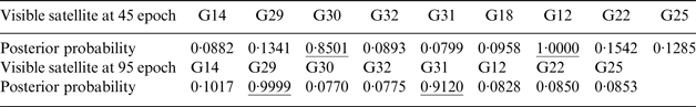
The experimental schemes are designed as follows. Firstly, we introduce two faults with sizes 40 m and 45 m in G30 and G12 at epoch 45, respectively. The visible satellites at epoch 45 are G14, G29, G30, G32, G31, G18, G12, G22 and G25. Secondly, we introduce two faults with the sizes 60 m and 35 m in G29, G31 at epoch 95, respectively. The visible satellites at epoch 95 are G14, G29, G30, G32, G31, G12, G22 and G25.
The posterior probabilities of the classification variables corresponding to the pseudo-range observations are shown in Table 3. The position errors before and after the faults exclusion are shown in Figures 7 and 8, respectively.
Figure 7. The position errors before faults exclusion.
Figure 8. The position errors after faults exclusion.
Table 3. The posterior probabilities of the classification variables corresponding to the pseudorange observations of the visible satellites at epoch 45 and 95.
From Table 3 it can be seen that the posterior probabilities of the classification variables corresponding to the pseudorange observations of G30 and G12 at epoch 45 are larger than 0·5, and the posterior probabilities of the classification variables corresponding to the pseudo-range observations of G29 and G31 at epoch 95 are larger than 0·5, which shows that the proposed method is capable of detecting multiple satellite faults in real data.
Comparing Figure 7 with Figure 8 it can be seen that the position errors are decreased.
6. CONCLUSIONS
A new Bayesian approach for multiple satellite faults detection and exclusion is proposed by introducing a classification variable to each satellite observation. If we treat this classification variable as random and assume a prior distribution for it, then a rule for satellite faults detection and exclusion based on the posterior probabilities of the classification variables is constructed under the framework of Bayesian hypothesis testing. A Gibbs sampler is introduced to compute the posterior probabilities of the classification variables, and the implementation for Bayesian RAIM algorithm combined with Gibbs sampler is designed.
Experiments illustrate that the algorithm proposed in this paper is convenient for implementation and capable of detecting and eliminating multiple satellite faults, whether under single constellation or integrated constellation. Many simulations indicate that the average number of iterations of the Gibbs sampler to achieve convergence is 200, the average computation time is 150 ms and the longest computation time is 230 ms, which shows that the proposed Bayesian RAIM algorithm can be implemented in real time. Also, the necessary time for outlier cancellation is almost within one epoch if the outlier is isolated.
The problems of assigning the prior distributions reasonably for the unknown parameters and making use of the historical information effectively need to be carefully studied in the future. It is expected that the algorithms proposed by this paper can be used to handle six or more outliers.
ACKNOWLEDGEMENTS
This research was supported jointly by National Science Foundation of China (No. 40974009, No.41174005), Planned Research Project of Technology of Zhengzhou City, and Funded Project with youth of Annual Meeting of China's satellite navigation.
APPENDIX
The derivation of Equation (17) is as follows. Firstly, according to the Bayes' theorem (Berger, Reference Berger1985; Koch, Reference Koch2007), we can obtain
 $$\eqalign{& p(\delta \vert X,\tau, L) \propto p(L\left\vert {X,\tau, \delta} \right.)p(\delta ) \cr & \quad \quad \quad \quad \quad \propto \prod\limits_{i = 1}^n {\displaystyle{1 \over {1 + \delta _i (k - 1)}}} \exp \left\{ { - \tau \displaystyle{{\sum\limits_{i = 1}^n {\displaystyle{{(L_i - a_i^T X)^2 p_i} \over {1 + \delta _i (k^2 - 1)}}}} \over 2}} \right\}\alpha ^{\sum\limits_{i = 1}^n {\delta _i}} (1 - \alpha )^{n - \sum\limits_{i = 1}^n {\delta _i}}} $$
Therefore,
 $$\eqalign{& p(\delta _i \left\vert {X,\tau,} \right.\delta _{( - i)}, L) \propto \displaystyle{1 \over {1 + \delta _i (k - 1)}}\exp \left\{ { - \displaystyle{{\tau (L_i - a_i^T X)^2 p_i} \over {2(1 + \delta _i (k^2 - 1)}}} \right\}\alpha ^{\delta _i} (1 - \alpha )^{ - \delta _i} \cr & \quad \quad \quad \quad \quad \quad \;\;\; \propto \displaystyle{1 \over {1 + \delta _i (k - 1)}}\exp \left\{ { - \displaystyle{{\tau \Delta _i^2 p_i} \over {2(1 + \delta _i (k^2 - 1)}}} \right\}\left(\displaystyle{\alpha \over {1 - \alpha}}\right)^{\delta _i}} $$
Further, according to the regularisation requirement of the probability density function, it is can be obtained that:
 $$\eqalign{& \tilde q_i = P(\delta _i = 1\left\vert {X,\tau,} \right.\delta _{( - i)}, L) = \displaystyle{{\alpha f\,({{\Delta _i \sqrt {\,p_i \tau}} / k})} \over {\alpha \varphi ({{\Delta _i \sqrt {\,p_i \tau}} / k}) + k(1 - \alpha )\varphi (\Delta _i \sqrt {\,p_i \tau} )}} \cr & \quad \quad \quad \quad \quad \quad \quad \quad \quad \quad \quad \quad \quad \quad \quad \quad \quad \quad \quad i = 1, \ldots, n} $$