Pricing Infrastructure-as-a-Service for online two-sided platform providers

Abstract

Infrastructure-as-a-Service (IaaS) is expected to grow at a rapid pace in the next few years. This is primarily because of the flexibility that it offers satisfying variable demand in computing power without any fixed investments in computing capacity. Our work focuses on a particular customer segment of IaaS – online platform providers (OPP). These businesses experience fluctuations in the number of users of their platforms, which impacts advertising revenues. Therefore, it is necessary for these businesses to support any sudden surge in demand without excessive upfront investments in computing infrastructure. IaaS offers an attractive option for such businesses. Pricing of IaaS for OPP is trickier as IaaS providers must consider the fluctuations in the number of users of such platforms while designing a plan. We model these fluctuations and their impact on the revenue of the platform providers to design an optimal pricing plan.

Appendix

Selection problem of online platform provider

Lemma 1:

• If q(ρ, σ) is the computing resource used by an OPP that has opted for an incentive compatible plan, then:

• a) (∂)/(∂ρ)(q(ρ, σ))⩾0

• b) (∂)/(∂σ)(q(ρ, σ))⩽0

Proof of Part (a):

• Let us assume (∂)/(∂ρ)(q(ρ, σ))<0, Therefore q(ρ, σ)>(q(ρ+∈, σ)) for ∈>0. As the plan is incentive compatible, from condition [IC],

Following condition [IC] for an OPP with revenue response ρ+∈ and user variability σ,

Adding up Inequalities (A.1) and (A.2) yields the following inequality:

Inequality (A.3), implies that (∂)/(∂σ)(U(q(ρ, σ), ρ, σ))⩽0 as q(ρ, σ)>(q(ρ+∈, σ)) − a contradiction of utility function property, which completes the proof. □

Proof of Part (b):

• Let us assume (∂)/(∂σ)(q(ρ, σ))>0. Therefore q(ρ+∈, σ)>q(ρ, σ) for∈>0. From condition [IC],

  

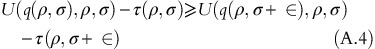
  Following condition [IC] for an OPP with revenue response ρ and user variability σ+∈,

  

  Adding up Inequalities (A.4) and (A.5) yields the following inequality:

  

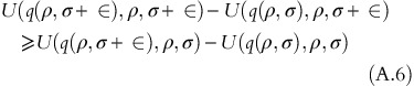
  Inequality (A.6) implies that (∂)/(∂σ)(U(q(ρ, σ), ρ, σ))⩾0 as q(ρ, σ+∈)>q(ρ, σ) − a contradiction of utility function property, which completes the proof. □

Selection of usage-based pricing policy

Lemma 2:

• If preference function of an OPP is defined as F(q(ρ, σ)ρ, σ)=U(q(ρ, σ), ρ, σ)−τ(ρ, σ), then:

• a) F(q(ρ, σ), ρ, σ) is strictly increasing in ρ.

• b) F(q(ρ, σ), ρ, σ) is non-increasing in σ.

Proof:

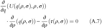
• Applying first order condition to satisfy condition [IC],

  
  

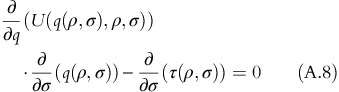
  Differentiating F(q(ρ, σ), ρ, σ) with respect to ρ yields:

  

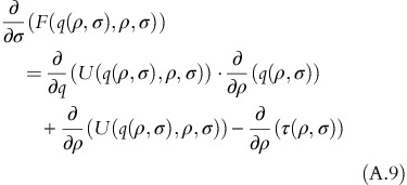
  Using the results obtained in equation A.7, equation A.9 results into:

  

  As(∂)/(∂σ)(U(q(ρ,σ),ρ,σ))>0,(∂)/(∂σ)(F(q(ρ,σ), ρ,σ))>0

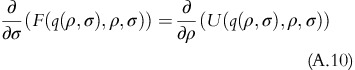
  To prove part (b), differentiating F(q(ρ, σ), ρ, σ) with respect to σ yields:

  

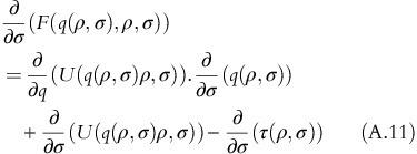
  Using the results obtained in Equation A.8, Equation A.10 results into:

  

  As (∂)/(∂σ)(U(q(ρ, σ), ρ, σ))⩽0, it shows that (∂)/(∂σ)(F(q(ρ, σ), ρ, σ))⩽0 □

Lemma 3:

• For limiting cases of user variability, if preference functions are defined as F ^L (q(ρ),ρ)=U ^L (q(ρ),ρ)−τ(ρ) and F ^H (q(ρ),ρ)=U ^H (q(ρ), ρ)−τ(ρ), then

• a) F ^L (q(ρ), ρ) is strictly increasing in ρ.

• b) F ^H (q(ρ), ρ) is strictly increasing in ρ.

Proof:

• Applying first order condition to satisfy condition [IC],

  

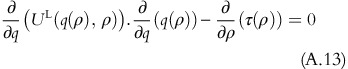
  Differentiating F^L(q(ρ),ρ) with respect to ρ yields:

  

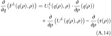
  Using equation A.13, equation A.14 can be rewritten as:

  

  As (∂)/(∂σ)(U^L(q(ρ), ρ))>0, it shows that (∂)/(∂σ)(F^L(q(ρ), ρ))>0 □

Part (b) can be established analogously.

Introduction of fixed-fee pricing policy

Lemma 4:

• If the fixed-fee surplus is defined as X(q(ρ, σ), ρ, σ)=V(ρ, σ)−U(q(ρ, σ), ρ, σ)+τ(ρ, σ), then

• a) X(q(ρ, σ), ρ, σ) is strictly increasing in ρ

• b) X(q(ρ, σ), ρ, σ) is strictly decreasing in σ.

Proof of Part (a):

• 

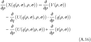
  From equation A.7, equation A.16 simplifies to:

  
  

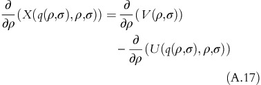
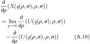
  As (∂²)/(∂q∂ρ)−(U(q(ρ, σ), ρ, σ))>0, it proves that (∂)/(∂σ)−(X(q(ρ, σ), ρ, σ))>0 □

Proof of Part (b):

• 

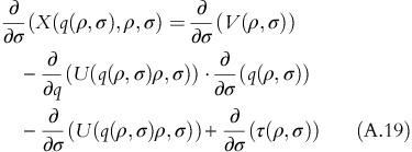
  From equation A.8, equation A.19 simplifies to:

  
  

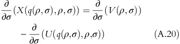
  As (∂²)/(∂q∂σ)(U(q(ρ, σ), ρ, σ))<0, (∂)/(∂σ)(X(q(ρ, σ), ρ, σ))<0□

Limiting cases

Lemma 5:

• For limiting cases of user variability, if fixed-fee surpluses are defined as X^L(q(ρ), ρ)=V^L(ρ)−U^L(q(ρ), ρ)+τ(ρ) and X^H(q(ρ), ρ)=V^H(ρ)−U^H(q(ρ), ρ)+τ(ρ), then

• a) X ^L(q(ρ), ρ) is strictly increasing in ρ

• b) X ^H(q(ρ), ρ) is strictly increasing in ρ.

Proof of Part (a):

• 

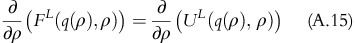
  From equation A.13, equation A.22 simplifies to:

  
  

  As (∂²)/(∂q∂ρ)(U^L(q(ρ,σ))>0, it proves that (∂)/(∂ρ)(X^L(q(ρ, σ))>0 □

Part (b) can be established analogously.

Proposition 2:

• Given an option to choose between two policies: usage-based and fixed-fee, OPP’s choice will follow the conditions given below:

• a) If or then all OPPs go for fixed-fee policy.

• b) If or then all OPPs go for usage-based policy.

• c) If and then OPPs with revenue responses will continue with usage-based policy whereas the OPPs with switch to the fixed-fee policy.

• d) If and then OPPs with revenue responses will continue with usage-based policy whereas the OPPs with switch to the fixed-fee policy.

• e) ρ _U ^H⩾ρ _U ^L

• f) ρ _S ^H⩾ρ _S ^L

Revenue responses ρ _U ^L and ρ _U ^H are defined as:

q*(ρ)=0∀ρ<ρ _U ^L when σ→0 and q*(ρ)=0∀ρ<ρ _U ^H when σ→∞.

Revenue responses ρ _S ^L and ρ _U ^H are defined as:

and

Proof of Part (a):

• Using results found in Lemma 5, fixed-fee surplus increases with increasing ρ for limiting conditions of user variability. Hence if an OPP with revenue response adopts fixed-fee policy, then all OPPs (with any ) will adopt fixed-fee policy because of higher fixed-fee surplus. This concludes the proof for Part (a) of Proposition 2. □

Proof of Part (b):

• Using results from Lemma 5, if an OPP with revenue response opts for usage-based policy, all OPPs will opt for the same policy because of decreasing fixed-fee surplus with decreasing ρ. This argument is valid for both limiting conditions of user variability. This concludes the proof. □

Proof of Part (c):

• From Lemma 5, X^L(q(ρ),ρ) and X^H(q(ρ), ρ) are increasing with . As OPPs with revenue response opt for usage-based policy, there will be a particular ρ at which X^L(q(ρ), ρ)=T. As ρ _S ^L and ρ _S ^H are the lowest such values of revenue responses for which X^L(q(ρ), ρ)=T and X^H(q(ρ), ρ)=T, all OPPs with ρ greater than these will opt for fixed-fee policy and the rest will go for usage-based policy. This concludes Part (c) of Proposition 2. □

Proof of Part (d):

• Let us assume that ρ _U ^H<ρ _U ^L.

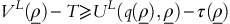
  From the definition of ρ _U ^H,

  

  Using the property of the utility functions for the limiting cases, for example, U^L(q(ρ), ρ)⩾U^H(q(ρ), ρ), we can write from equation A.25 that:

  

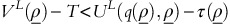
  From the definition of ρ _U ^L it follows that:

  

  As ρ _U ^H<ρ _U ^L and F^L(q(ρ), ρ) is strictly increasing with ρ, equations A.26 and A.27 contradict each other. Hence by contradiction it is proved that ρ _U ^H⩾ρ^L _U . □

Proof of Part (e):

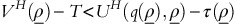
• Let us assume that ρ _S ^H<ρ _S ^L. From the property of ρ _S ^L,

  
  

  As (∂²)/(∂q∂σ)(U(q(ρ,σ),ρ,σ))<0, equation A.29 can be expressed as:

  

  As ρ _S ^H<ρ _S ^L,

  

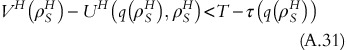
  equation A.31 contradicts the definition of ρ _S ^H, hence ρ _S ^H⩾ρ _S ^L. □

Optimal usage-based pricing policy by IaaS providers

Proposition 3:

• The optimal quantity (q*(ρ, σ)) and corresponding price (τ(q*(ρ, σ))) is determined by the following set of expressions:

  
  

  ρU is the value of revenue response below which the amount of computing resource, q is zero, irrespective of the value of σ. Similarly, σ _H is the value of user variability above which the amount of computing resource q is zero, irrespective ofthe value of ρ.

Optimal computing resource is calculated by solving the following unconstrained optimization problem:

Optimal pricing policy for optimal quantity of computing resource (q*(ρ, σ)) is defined by the following expression:

Density functions of revenue response and user variation for different OPPs are characterized as h(ρ) and g(σ). Individual rationality condition is satisfied in following ranges of ρ and and .

Proof:

• Optimality conditions for incentive compatibility: □

IC condition is satisfied when p, σ are solutions to the following maximization problem:

From the first order conditions:

Every OPP with and will follow the above two expressions and it leads to the following set of equations:

From the second order conditions, H _xx <0, H _yy <0 and determinant of Hessian matrix should be non-negative. H _xx and H _yy are determined by differentiating equations A.36 and A.37 with respect to x and y.

Substituting ρ and σ as solutions in equation A.40,

Differentiating equation A.38 with respect to ρ and substituting the expression of ∂²/∂ρ²(τ(ρ, σ)) into equation A.43 gives:

As ∂²/∂q∂ρ(U(q(ρ, σ),ρ, σ))>0, equation A.44 gives ∂/∂ρ(q(ρ, σ))>0, which is established in Lemma 1. Substituting ρ and σ as solutions in equation A.41,

Differentiating equation A.39 with respect to σ and substituting the expression of ∂²/∂σ²(τ(ρ, σ)) into equation A.45 gives:

As ∂²/∂q∂σ(U(q(ρ,σ),ρ,σ))<0, equation A.45 gives ∂/∂σ(q(ρ, σ))<0, which is established in Lemma 1.

We substitute ρ and σ while calculating the determinant of the Hessian matrix. ∂²/∂ρ∂σ(τ(ρ, σ)) and ∂²/∂σ∂ρ(τ(ρ, σ)) are calculated by differentiating equation A.38 with respect to σ and by differentiating equation A.39 with respect to ρ and corresponding expressions are substituted in Hessian matrix. The determinant of the Hessian matrix comes to zero. Equating ∂²/∂ρ∂σ(τ(ρ, σ)) and ∂²/∂σ∂ρ(τ(ρ, σ)), we get the following condition of optimality:

Redefining the objective function of IaaS provider:

Informational rent of an OPP with ρ and σ is defined as:

Differentiating equation A.48 with respect to ρ,

Using equation A.38, equation A.49 is rewritten as,

Differentiating equation A.48 with respect to σ,

Using equation A.39, equation A.51 is rewritten as,

Differentiating equation A.50 with respect to σ and equation A.52 with respect to ρ yields:

The second equation follows from the optimality condition given in equation A.47. We take the IR satisfied for and . Using this condition,

From equation A.48,

Objective function of IaaS provider:

Objective function of IaaS provider to maximize profit,

Substituting the expression of τ(ρ, σ) from equation A.56,

Assuming independence of density functions, that is, f(ρ, σ)=h(ρ)g(σ), objective function becomes,

with E(ρ, σ) is defined as:

Hence,

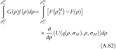
Expanding the second part of the integral defined in equation A.60 and using integration by parts, ∫udv=uv−∫vdu, with u=E(ρ, σ) and v=G(σ),

Substituting expression of dE(ρ,σ) from equation A.62, equation A.63 can be rewritten as:

Inserting the expression of integra into equation A.60, objective function becomes:

□

Optimal pricing structure in the presence of fixed-fee

Proposition 5:

• For an OPP with user variability σ _M , if we assume that the OPP shifts to fixed-fee plan from the usage-based plan at a revenue response of ρ _M , where ρ _M ∈[ρ _S ^L, ρ _S ^H], then the optimal combination of usage-based fee and fixed-fee can be determined as follows.

• a)
  
• b)
  

• c) T^*=V(ρ _S ^M*,σ _M )−U(q*(ρ _S ^M*,σ _M ), ρ _S ^M*,σ _M )+τ*(ρ _S ^M*,σ _M ). Here q*(ρ, σ) is the optimal quantity and τ(q*(ρ,σ)) is the corresponding price (Proposition 3).

Proof:

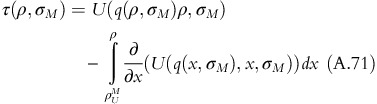
• Informational rent of OPPs with ρ and σ _M is defined as:

  

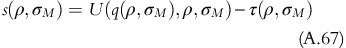
  Differentiating with respect to ρ yields

  

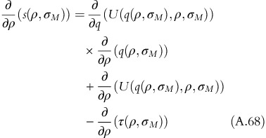
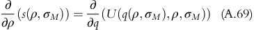
  Using equation A.38, equation A.68 can be written as,

  

  We consider a revenue response ρ _U ^M∈[ρ _U ^L, ρ _U ^H] at which the OPP adopts the usage-based plan. Below p _U ^M, the OPP would not be interested in adopting a usage-based plan. Hence,

  

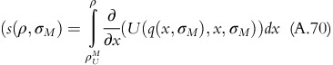
  Hence,

  

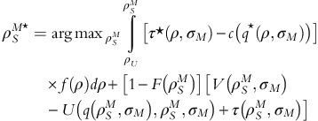
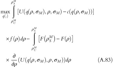
  The objective function of IaaS provider becomes:

  
  
  

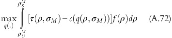
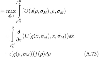
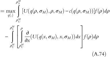
  Defining

  

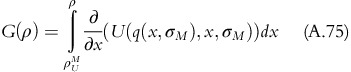
  Equation A.74 can be written as

  

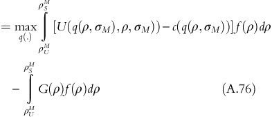
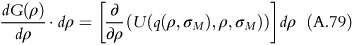
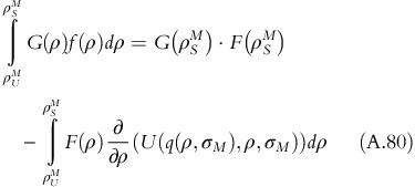
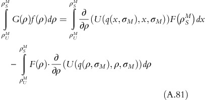
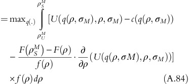
  Using integration by parts, ∫udv=uv−∫vdu where u=G(ρ), v=F(ρ), dv=f(ρ)dp we get,

  
  

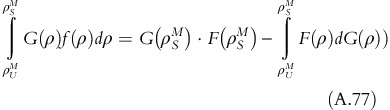
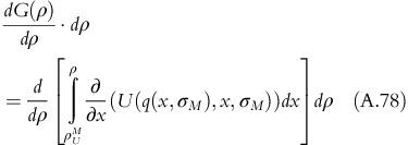
  Applying Leibnitz rule,

  
  
  
  

  Therefore, the objective function becomes,

  
  

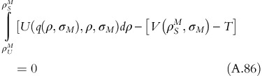
  Now, if we introduce fixed-fee T, the objective function becomes,

  

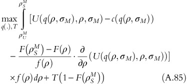
  subject to

  

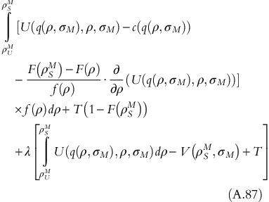
  The constrained optimization problem is represented as Lagrangian problem: L(q(.), T, λ)

  

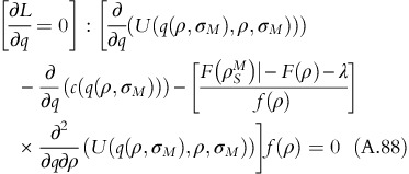
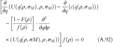
  FOC of the Lagrangian problem:

  
  
  

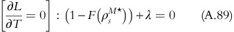
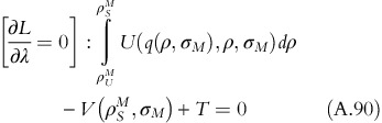
  From equation A.89,

  

  Substituting the value of λ in equation A.88 gives

  
  

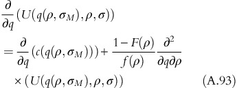
  This expression shows that optimal usage-based quantity q*(ρ, σ _M ) in independent of ρ _U ^M, ρ _S ^M and T.

  Corresponding ρ _S ^M value is

  

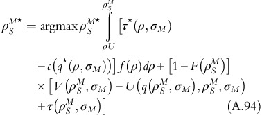
  The optimal fixed-fee T* is given by

  

   □

References

Anandasivam, A. and Weinhardt, C. (2010) Towards an effcient decision policy for cloud service providers. In: ICIS 2010 Proceedings, Saint Louis, Missouri, USA.
Bagh, A. and Bhargava, H.K. (2013) How to price discriminate when tariff size matters. Marketing Science 32 (1): 111–126.
Bakos, Y. and Brynjolfsson, E. (1999) Bundling information goods: Pricing, profits and efficiency. Management Science 45 (12): 1613–1630.
Bala, R. and Carr, S. (2010) Usage-based pricing of software services under competition. Journal of Revenue and Pricing Management 9 (3): 204–216.
Bashyam, T.C.A. (2000) Service design and price competition in business information services. Operations Research 48 (3): 362–375.
Cocchi, R., Shenker, S., Estrin, D. and Zhang, L. (1993) Pricing in computer networks: Motivation, formulation and example. IEEE/ACM Transactions on Networking (TON) 1 (6): 614–627.
Dewan, S. and Mendelson, H. (1990) User delay costs and internal pricing for a service facility. Management Science 36 (12): 1502–1517.
Fudenberg, D. and Tirole, J. (1991) Game Theory. Cambridge, MA: MIT Press.
Gannes, L. (2010) How zynga survived farmville. http://www.gigaom.com, accessed 25 July 2013.
Gupta, A., Stahl, D. and Whinston, A. (1996) Economic Issues in Electronic Commerce. Reading MA: Addison Wesley.
Hilton, S. (2010) Cloud computing is no fad. http://www.forbes.com, accessed 25 July 2013.
Jain, S. and Kannan, P. (2002) Pricing of information products on online servers: Issues, models and analysis. Management Science 48 (9): 1123–1142.
Li, C. (2011) Cloud computing system management under at rate pricing. Journal of Network and Systems Management 19 (3): 305–318.
Kahin, B. and Keller, J. (eds.) (1995) Public Access to the Internet. New York: The MIT Press.
Marston, S., Li, Z., Bandyopadhyay, S., Zhang, J. and Ghalsasi, A. (2011) Cloud computing – The business perspective. Decision Support Systems 51 (1): 176–189.
Maskin, E. and Riley, J. (1984) Monopoly with incomplete information. Rand Journal of Economics 15 (2): 171–196.
Mendelson, H. (1985) Pricing computer services: Queueng effects. Communications of the ACM 28 (3): 312–321.
Mendelson, H. and Whang, S. (1990) Optimal incentive-compatible priority pricing for the M/M/1 queue. Operations Research 38 (5): 870–883.
Parker, G. and Alstyne, M. (2005) Two-sided network effects: A theory of information product design. Management Science 51 (10): 1494–1504.
Shapiro, C. and Varian, H. (1999) Information Rules. Boston, MA: Harvard Business Review Press.
Stosser, J. and Neumann, W.C.D. (2010) Market based pricing in grids: On strategic manipulation and computational cost. European Journal of Operations Research 203 (2): 464–475.
Sundararajan, A. (2004) Nonlinear pricing of information goods. Management Science 50 (12): 1660–1673.
Varian, H. (1995) Pricing information goods. In: Proceedings of Scholarship New Inform. Environment Symposium. Harvard Law School, Cambridge, MA.
Varian, H. (2009) Intermediate Microeconomics: A Modern Approach, 8th edn. New York: W.W. Norton & Company.
Wilson, R. (1993) Nonlinear Pricing. New York: Oxford University Press.
Author information
Authors and Affiliations
Corresponding author