
ABSTRACT
We describe a method to quantify the degree of parallelism between two transparent glass mirrors spaced a few microns apart. Our technique, which permits the measurement and correction of deviations as small as λ/10000 from parallelism, is fundamental to the successful operation of tunable narrowband interference filters for two reasons. First, the highest throughput is achieved when the plates are parallel at any plate spacing. Second, the lowest resolution (largest bandpass) imaging is achieved when the plates are only a few microns apart, but there is a real danger of the plates touching if parallelism is not maintained. The Taurus Tunable Filter (TTF)3 is a Fabry‐Perot cavity with an adjustable plate spacing of 2–13 μm. The parallelism measurement involves repeated imaging through a focal‐plane slit and a series of pupil‐plane masks. This approach is particularly efficient when the plate scanning is synchronized with the movement of the charge on the CCD. We assess the effects of wavelength‐dependent phase changes within the inner surface coatings of the plates. These become important as the plates approach a spacing comparable in size to the thickness of the coatings.
Export citation and abstract BibTeX RIS
1. . INTRODUCTION
Fabry‐Perot interferometers have long been used in astronomy as a means of obtaining narrowband imaging of galaxies and nebulae (q.v. Bland‐Hawthorn 1995). However, with typical plate spacings in the range ∼20–500 μm, optical instruments have been confined to high orders of interference (m ∼ 50–2000). Most work is therefore restricted to relatively high resolution (λ/δλ>1500), where the interference rings are narrow and cover only a small area on the detector. For astronomical work, the drawback of this type of imaging is that interference regions consequently cover only a small solid angle on the sky.
To solve this problem, we have successfully commissioned a narrow‐gap Fabry‐Perot interferometer called the Taurus Tunable Filter (TTF; Bland‐Hawthorn & Jones 1998), which is based on a design originated by Atherton & Reay (1981). This filter consists of two parallel glass plates with an adjustable gap spacing of 2–13 μm. Two recent advancements have led to the development of this instrument. First, multilayer dielectric coatings are now able to cover 300 nm or more with transmissions of 99% or better. Second, it is now possible to drive Fabry‐Perot interferometers to gap spacings as small as 1 μm, which requires that the cavity spacing be kept clean of even a single dust speck. The dynamic range of accessible plate spacings is much broader than earlier instruments because of developments in stacked piezo‐electric transducers (PZTs). These permit the TTF to scan through a range of spacings 4 times larger than that accessible by conventional Fabry‐Perot spectrometers. Unlike the instrument of Atherton & Reay (1981), the TTF coatings of each surface are polished to a flatness better than λ/140 (post coating) and optimized for ∼300 nm wavelength coverage for both the red and blue arms. The tunable filter is used in conjunction with high‐performance, large‐format (e.g., MIT‐LL 4096 × 2048) CCDs. Alternative tunable devices such as acousto‐optic or birefringent filters do not currently match the qualities that make the Fabry‐Perot system most desirable for astronomical imaging (Bland‐Hawthorn & Cecil 1996).
The combination of moderate‐telescope f‐ratio (f/8) and narrow‐gap spacing of TTF means that the requirement for large‐area interference is met. However, ensuring parallelism of the plates becomes increasingly critical at the limit of narrow spacings. For conventional instruments, parallelism can be judged by eye according to how stable the interference rings from a monochromatic source remain with changes in viewing position. This approach works well at visible wavelengths for Fabry‐Perot interferometers with widely spaced plates. For plates that are narrowly separated, the order of interference is too low (typically m≲20), and since the field is essentially monochromatic, it fails to provide the sharp rings necessary for visual assessment over a light table.
To overcome this, we have developed a test that efficiently optimizes plate parallelism up to λ/10000. This limit is defined by the smallest deviation that we can both measure and correct, as derived in § 3.2. Our test is effective over the full range of TTF spacings down to 2 μm. Alternative techniques for measuring parallelism, such as beam partitioning by insect‐eye lenses (Meaburn et al. 1976), were explored and found impracticable for an astronomical imager such as TTF. A novel CCD charge‐shuffling technique is employed that involves multiply exposing a single CCD image during the test. This avoids the need to produce many separate CCD images.
At the narrowest spacings, we are in a regime where deviations from phase change on reflectance are important. This occurs as the gap size becomes comparable to the thickness of the inner optical coatings. Each 16‐layer dielectric has a total thickness of 1.55 μm. Nonuniformities in the coating structure also become apparent as the plate spacing approaches this limit. In particular, the interference fringes deviate from circular symmetry. We calculate the effects of this phenomenon across scans at the narrow‐gap limit of our instrument. The wavelength‐dependent phase changes and nonuniformities are negligible at a large gap.
This paper is organized as follows. The experiment layout and operation are detailed in § 2. A description of the parallelism test is given in § 3, including the effect of phase changes within the plate coatings. Section 4 contains concluding remarks.
2. . SETUP AND OPERATION
2.1. . Charge Shuffling
Charge shuffling is the ability to multiply, expose, and shift an individual CCD frame backward and forward along the chip many times before readout. With the AAO‐1 controller and a MIT‐LL CCD, a single row of 2048 pixels can be shuffled one row in 50 μs, whereas to read out the same row takes 40 ms. This technique has been used with TTF at the Anglo‐Australian Observatory since 1994.
Charge shuffling is essential to effective parallelism testing since it provides a powerful tool for sampling TTF throughput as it is stepped over successive gap spacings, without the need for many discrete CCD images. Similar charge‐shuffling methods have been applied to other forms of astronomical imaging such as the imaging polarimetry (Clemens & Leach 1987) and spectroscopy of faint galaxies (Cuillandre et al. 1994). Bland‐Hawthorn & Jones (1998) describe more sophisticated charge‐shuffle applications with TTF.
We use both the MIT‐LL 4096 × 2048 (rows × columns) CCD with 15 μm pixels and a 1024 × 1024 Tektronix CCD with 24 μm pixels. Both are buried‐channel devices with charge transfer efficiencies in excess of 0.99999. Tests involving repeated shuffling with the Tektronix chip have demonstrated that 100 full‐frame shuffles are possible before significant charge‐loss occurs (Bland‐Hawthorn & Jones 1998). Bulk traps are the major cause of charge loss, arising from impurities and defects within the silicon lattice of the CCD (Janesick & Elliott 1992). The missing charge leaks out of trailing pixels as a deferred charge or is lost through recombination. The TTF plate spacing can be also be changed and allowed to settle within the time of a single shuffle (50 μs). The primary limitation to shuffle speed is the shutter, which keeps the rate at 1 s for one complete shuffle.
2.2. . Pupil Hartmann Test
The parallelism test employs an identical optical arrangement to that for astronomical imaging, with the exception of masks added at the focal and pupil planes. Figure 1 shows the main components of the system. Our basic method is to irradiate the TTF with a monochromatic source. In the focal plane, we use a slit that projects to a few rows of the CCD. The slit mask ensures that only a thin strip of monochromatic light is imaged at the center of the CCD detector. The tunable filter is located in a collimated beam, and quadrant‐shaped masks placed in the pupil plane isolate a quarter of the TTF plate area at a time for testing.
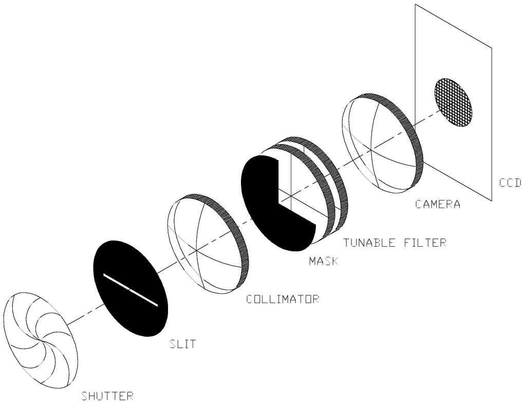
Fig. 1.— Arrangement of components in the optical train for pupil‐plane quadrant imaging. Only the slit and quadrant masks need to be removed to ready the system for astronomical imaging.
The long‐slit spectra used for determining parallelism are obtained in the following manner. An exposure is taken, at the end of which the shutter is closed, the TTF plates shift to the next value of plate spacing, and the current frame in the CCD is shifted by a small amount. The shutter is then reopened for the next exposure, sampling the light source at the new spacing. The CCD is multiply exposed 100–200 times before it is eventually read out. This produces a long‐slit spectrum similar in appearance to that obtained from a grating spectrograph. The method can be sped up by keeping the shutter open and shuffling the charge during the exposure. But a significant time constant, which determines the settle time of the plates, can lead to a spurious phase offset.
Figure 2 shows an example of a long‐slit spectrum of a Cu‐Ar lamp obtained using the red TTF and charge shuffling with the Tektronix CCD. The spectrum covers 730–788 nm and comprises 80 discrete shuffle exposures, only covering the top half of the CCD. This is true for the following reason: a fraction (n - 1)/(2n - 1) of the detector area must be sacrificed in a shuffle of n rows to allow space for the spectrum to be shuffled along as it is built. The lines are narrow because the TTF was set to a large gap (12 μm). The curvature of the lines is due to the combined effects of radial phase change and a scan increment. It is emphasized at a large gap (higher orders of interference) or when small increments in spacing are used between successive shuffles. Once parallelism has been established at large spacing, the plates retain their alignment irrespective of how TTF is tuned thereafter.
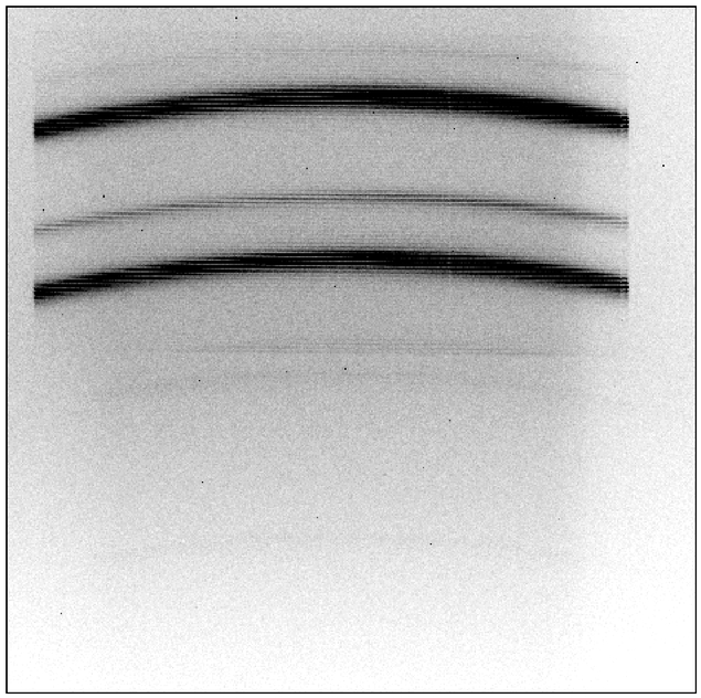
Fig. 2.— Charge‐shuffled long‐slit spectrum of a Cu‐Ar lamp over 730–788 nm. The lines (from top to bottom) are shown at 750.90 (doublet), 772.40 (doublet), and 763.51 nm. The wavelength does not increase sequentially along the frame due to wraparound of the adjacent orders.
As shuffling is ordered top to bottom, the row number on the image is linearly related to increasing gap spacing between the plates. However, this does not necessarily imply that wavelength is strictly increasing over a full shuffle. Occasionally, wavelength wraparound occurs between adjacent orders of interference. To remove this confusion, we typically observe through two orders of interference.
2.3. . Control of TTF Plates
For peak performance of a Fabry‐Perot device, the error in plate parallelism must be much less than the deviations from the flatness in the plate surface. The coated plates in TTF are individually flat to λ/140, and normally parallelism must be established and maintained to at least λ/500 during use. To achieve this, the plates of TTF are controlled through an active feedback loop that constantly corrects the plates when small changes from plate position occur (Hicks & Atherton 1997; q.v. Ramsay 1962). Such closed‐loop control is essential for a device such as TTF, where plate stability could otherwise be influenced by variations in temperature, humidity, and gravity on the plates as the telescope moves.
Hicks, Reay, & Atherton (1984) pioneered the technique of Fabry‐Perot stabilization using a capacitance bridge. Their Figure 1 shows the components employed in the active feedback system used by TTF. Four capacitors around the edge of the inner‐plate surfaces (labeled in their Fig. 1 as CX1, CX2, CY1, and CY2) detect changes in plate spacing. Such changes permit the measurement of the plate tilt along the direction of the x‐ and y‐axes defined by the two capacitor pairs. This capacitance micrometry is capable of detecting displacements of 10−12 m (Jones & Richards 1973). Tilt information from the capacitors is fed to PZTs that compensate for the amount of deviation. There are three PZTs, each located around the plate edge between the capacitors and separated by 120°. An additional reference capacitor measures the gap spacing with respect to a fixed capacitor built onto one of the plates.
When the plates are parallel, capacitance will not be equal between either the CX1, CX2 or the CY1, CY2 pairs. This is why the feedback system can only maintain parallelism and not establish it in the first place. Electronic offsets are applied to compensate for variations in capacitance whenever they occur. These can arise from temperature gradients across the Fabry‐Perot interferometer or continual changes in the piezo dimensions due to creep in the PZT lattice structure. All such capacitance changes are continually balanced and nulled automatically by the system electronics.
We are able to introduce fixed vertical offsets ZX and ZY along the x and y directions through three levels of control: coarse, fine, and software. Both coarse and fine controls are analog inputs directly through the hardware of the TTF controller. The software control allows the precision adjustment of the plates via digital input. The maximum ZX and ZY amplitudes are 3.21 μm. Clearly, it is crucial to ensure that the plates are parallel before attempting to achieve gaps smaller than about 7 μm. The vertical deviation along the x‐axis from the zero point is given by
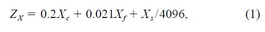
where ZX is in units of microns and Xc, Xf, and Xs are the respective coarse, fine, and software settings in X. Each control has its own range:Xc∈[-5, +5], Xf∈[0,10], and Xs∈[-2048, +2048]. An identical calibration relates ZY with Yc, Yf, and Ys across identical settings.
No gap scanning is done through the ZX or ZY movements. They are purely offsets that remain fixed unless adjusted for parallelism. Scanning is controlled through a third parameter Z, which has the much larger amplitude of 13.05 μm. It too can be adjusted through three levels of coarse, fine, and software control:

although with a much larger range in the coarse setting than ZX or ZY. Equation (2) is the absolute calibration used to tune the plates to an arbitrary gap (and therefore wavelength) during normal observing. It depends on the values of (Xc,Xf,Xs) and (Yc,Yf,Ys) at the time of calibration; in the case of equation (2), for the TTF, (Xc,Xf,Xs) = (0.0,3.90,0.0) and (Yc,Yf,Ys) = (0.1,8.00,0.0). Although the setting limits of Zc, Zf, and Zs are identical to those of x and y, the corresponding physical ranges are much larger. Since Zc and Zf are analog controls, all gap scanning is done through the automated stepping of Zs in software. The units of Z in equation (2) are in microns. The amount of offset is derived directly from the parallelism test and refined through successive iterations. We describe the test in the following section.
3. . PARALLELISM TEST
3.1. . Method
The X‐Y capacitive bridges define the direction of the orthogonal x‐ and y‐axes. We assume that all components are located central to the beam, although this alignment is not critical. Only three of the four possible quadrants are needed to establish the magnitude and direction of the plate tilt. In any such arrangement of quadrants, we define the corner quadrant to be the reference quadrant and the remaining pair as the X and Y quadrants according to their direction from the reference.
We image an emission line by scanning through each quadrant in turn, producing a charge‐shuffled long‐slit spectrum for each. The amount of tilt is measured by the size of the offset between the line through the X or Y and the reference quadrant. The plates are parallel when no offsets exist in either direction and when the emission line appears simultaneously in all three.
Figure 3 shows how the adjustment of the capacitive offsets optimizes plate separation. Here identical central strips have been taken from a full charge‐shuffle image (such as Fig. 2). The X, Y, and reference quadrants are labeled. Each shuffle step represents an increase in plate spacing of 8 Å or ∼λ/1140. Panel (a) shows a small offset in Y only (arrow). This implies that the plates are tilted in the y‐direction but not in the x‐direction. In the following section, we demonstrate how this offset in gap is proportional to the compensatory offsets that are input. Note that the calibration source seen in Figure 3 is poorly diffused over the entrance aperture and that differences in illumination between quadrants are present.
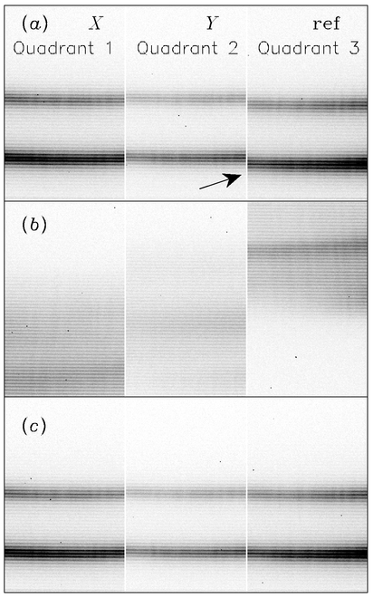
Fig. 3.— Demonstration of how plate tilts are measured and adjusted using three quadrant masks. Only the central portions of each full charge shuffle image are shown, and each shuffle step is an increase of 8 Å or ∼λ/1140. Panel (a) indicates a small offset in the y‐direction only. Panel (b) shows the degraded appearance of lines at much larger offset. Panel (c) demonstrates the alignment of all lines and the attainment of parallelism. The uneven illumination between panels is due to the poorly diffused internal lamp.
Panel (b) shows the appearance of the lines when the plates are more poorly aligned. Not only are the lines misaligned in this case but much less distinct as well. Preliminary adjustments such as those between (a) and (b) are used to establish the directional relationship between offset voltage and tilt. Having the pupil masks telecentric, with quadrant edges aligned to the x‐ and y‐axes, greatly simplifies the process.
The remaining fine adjustment of the plates is an iterative process whereby piezo offset voltages are adjusted through the software control until the wavelength offsets between all quadrants are zero. The alignment of all lines in (c) indicates the plates to be parallel. This ensures that the effective finesse and throughput of the instrument are now optimized.
3.2. . Deriving a Corrective Offset
We now derive the relationship between a directional offset (as measured optically near the centers of each quadrant) and the corrective offset (as it applies in the vicinity of the capacitors and PZTs). This is necessary because the offsets for a tilted plate are measured and corrected in two different locations, namely, the center and edge of the plate, respectively.
Let us suppose the upper plate is tilted along the plane

relative to the lower plate at z(x,y) = 0. Here L0 is the separation of the plate centers (in units of microns), and A and B are constants proportional to the slope in x and y. We assume that the x‐ and y‐axes align with the XY capacitors and that the p‐ and q‐axes define the four segments of the pupil‐plane masks. Initially, we also assume the p‐ and q‐axes to be rotated an angle φ counterclockwise from the positive x‐axis.
The location of emission lines (such as those in Fig. 3) determines the effective plate separation over that region. The effective plate separation is the volume of space between the plates divided by the cross‐sectional beam area isolated by the quadrant mask. Integrating over each quadrant in turn gives effective plate separations:
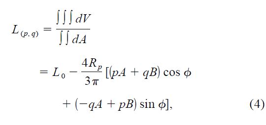
where (p,q)∈{(± 1, ± 1)} and have values according to what region the quadrant occupies of the (p,q)‐plane (Fig. 4, inset). The beam radius, Rp, is defined by the radial size of the beam at the pupil plane (37.75 mm).
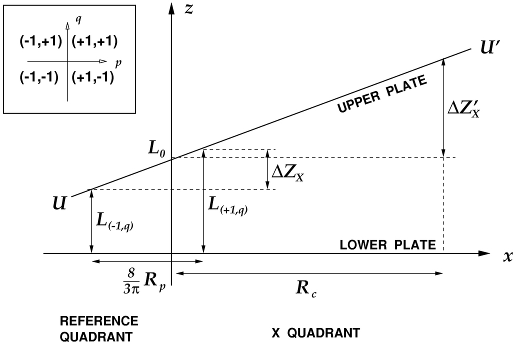
Fig. 4.— A side view showing the parameters that quantify plate tilt in the x‐direction. The convention used in labeling quadrants by their (p, q) ∈ {(±1, ±1)} value is also shown (inset).
The problem is much simplified if the quadrant masks are oriented such that the edges are parallel with the x‐ and y‐axes. This is how our system is operated in practice, deliberately decoupling the XY tilt motions. In the absence of rotation, equation (4) reduces to
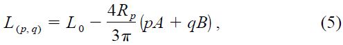
with (p,q)∈{(± 1, ± 1)} according to quadrant, but where the p‐ and q‐axes and the x‐ and y‐axes are now aligned. Equating equations (3) and (5) gives the linear locus of points across a quadrant (p,q) at which the plates are separated by exactly L(p,q),
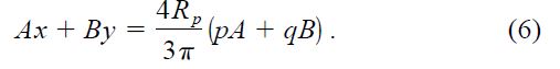
Now let us consider any two quadrants that are adjacent in the x direction (that is, with common q but opposite p values). It can be shown by equation (6) that the separation (in x) between the L(p,q) loci of both quadrants remains fixed at 8Rp/3π for all values of y. In other words, the baseline separating L(-1,q) and L(+1,q) in the x‐direction is a constant, irrespective of y. The same is true for loci separation in the y‐direction along lines of constant x.
Figure 4 shows a side view along the x‐direction of an upper plate (UU') tilted relative to a lower one (x‐axis). L(-1,q) and L(+1,q) are the effective plate separations measured in each quadrant, while ΔZX is the difference between the two. Without loss of generality, we set the reference quadrant to be on the negative side and the X‐quadrant on the positive. The offset ΔZ'X is the amount by which the plate needs correction at the radius of the PZTs and capacitors, Rc. From Figure 4, we know through geometrical argument that
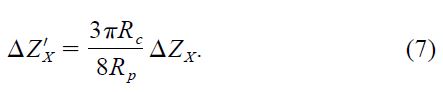
We show in Figure 3 how an offset such as ΔZX can be measured directly by the offset of lines (panels X and ref in the case of the x‐offset).
Substituting the radii of the pupil‐plane beam (Rp = 37.75 mm) and PZTs (Rc = 90 mm) in equation (7) yields
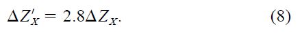
This is the relationship we need between measured offset, ΔZX, and applied (corrective) offset, ΔZ'X. It means that any measured offset in the x‐direction must be corrected by 2.8 times that offset in the opposite direction. Similar arguments find an identical scale factor between ΔZY and ΔZ'Y. The units in equation (8) can be either the measured software control units or the physical units (μm) through equation (1).
The precision of the technique is limited to the smallest steps by which the plates can be adjusted, not the smallest measurable deviation. By equation (1), the smallest movement is a software step of 1, equivalent to ΔZ'X = 0.24 nm or ∼0.01% of our smallest plate spacing. This we can detect through motions as small as 0.09 nm near the plate center. At the longest wavelengths, this represents λ/10000. This is much less than the λ/500 parallelism criterion, over the full range of TTF wavelengths.
3.3. . Reflectance Phase at Narrow Gap
The condition for maximal transmission of light with wavelength λ through a Fabry‐Perot interferometer is
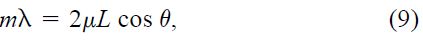
where m is the order of interference, L is the spacing between the plates, θ is the interior angle of incidence, and μ is the refractive index of the gap medium. For TTF, this medium is air with μ = 1.00. Equation (9) is an approximation suitable for high orders and therefore large plate spacings. However, it fails to take into account the wavelength‐dependent phase change inherent in reflections between the optical coatings on the inner‐plate surfaces. Such coatings are optimized to reflect the design wavelength (819 nm for TTF) with zero phase change, but they incur a lead or lag phase elsewhere. The phase change becomes increasingly important as the plate spacing becomes comparable to the thickness of the optical coatings.
Equation (9) can be modified to
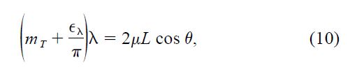
accounting for phase change through the introduction of an order correction term,  λ (Atherton et al. 1981; Knudtson, Levy, & Herr 1996). Here mT is the true order number associated with phase correction. The subscript λ denotes the wavelength dependence of . At large orders mT, the effect of the phase change term becomes negligible. The inner coatings of the red TTF cause λ to vary by ±π over 630–950 nm.
The ratio mT/m characterizes the relative influence of phase change at a given wavelength. Combining equations (9) and (10) for a common wavelength and plate spacing L gives
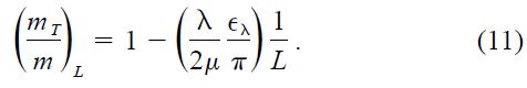
By this, we see that the relative size of the phase correction will become larger toward smaller gap at a given wavelength. In practice, the phase correction will also alter the free spectral range and bandpass of the instrument, in addition to the shape and location of the transmission profile (Atherton et al. 1981). Table 1 contains a list of λ/π values at selected wavelengths, as measured by Queensgate Instruments. The values for the coefficient in equation (11) are also included.
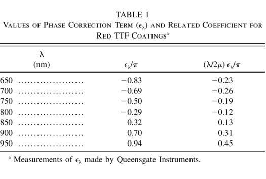 |
Figure 5a shows four TTF scans at the lowest plate spacings reached by our instrument. The scans show blended lines of Ne (659.9, 667.8, and 671.7 nm). The lines are unresolved at all plate spacings except the largest (L = 4.7 μm), where they are labeled. The scans were made at various values of (Zc,Zs) and transformed to physical units of spacing by equation (2). Changes in the software scan increment (ΔZs) are evident in the different sampling densities of each scan. Let us observe that the transmission peaks are evenly separated by λ/2μ = 0.33 μm, confirming that the calibration in equation (2) is robust over all settings of Zc and Zs used. Also note the broadening of the transmitted profile as plate spacing and resolution decreases. The flat background levels are from CCD regions that were not used in the charge shuffle.
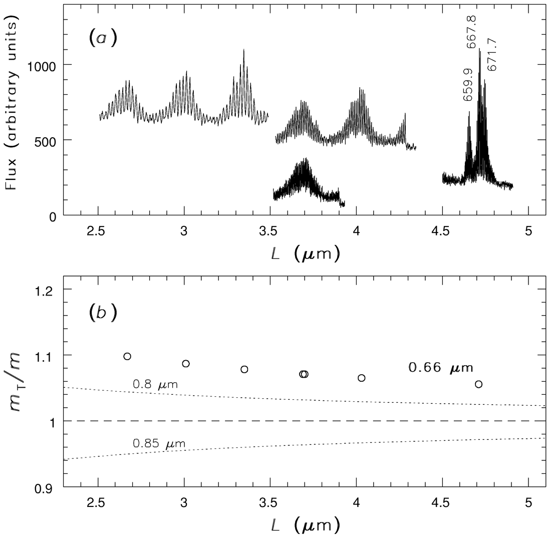
Fig. 5.— (a) Four scans of blended Ne lines at the narrowest TTF plate spacings. The lines are only partially resolved at the largest gap and have been labeled with their wavelengths in units of nanometers. (b) Values of mT/m for the orders measured in (a). The rise in this ratio toward a lower gap demonstrates the increasing importance of wavelength‐dependent phase change at the lower limits of the TTF operation. The dotted lines show mT/m calculated for wavelengths of 0.8 and 0.85 μm.
In Figure 5b, we plot the change in mT/m for the same orders of the Ne blend shown in Figure 5a. The ratio mT/m was calculated at each plate spacing measured in Figure 5a by equation (11). Queensgate Instruments have measured λ = -0.79π for TTF at 666 nm. Let us observe in Figure 5b that phase correction is a ∼10% effect at 670 nm. The dotted lines show the effect to be significantly less at wavelengths near the center of the TTF coverage. The narrowest spacing (2.5 μm) is a self‐imposed limit to which we are prepared to drive the plates. If it were any closer, we would run the risk of damaging the inner coatings by pressing dust particles between the two coating surfaces. We conclude that at the narrowest spacings of TTF, we are in a regime where phase effects are nonnegligible, particularly for wavelengths at the extremities of the optical coating curve.
4. . SUMMARY AND FUTURE WORK
We have resolved a major hurdle to Fabry‐Perot tunable filters finding wider use at major observatories. The pupil Hartmann test described here is fundamental to the application of tunable filters, particularly at the lowest resolutions (smallest gaps). Our method is sensitive to deviations as small as λ/10000 over the optical range. Clearly, this technique has far wider applications in precision measurements of flatness.
The Hartmann test achieves plate parallelism across the full 11 μm scan range of the TTF. This has encouraged us to bring the analog (CS‐100) control system under full electronic control. In the past, switching in hardware to different parts of the physical scan range induced a small random offset in the wavelength‐gap calibration after returning to a former coarse setting (see § 2.3). Another benefit is "broad‐narrow" shuffling since frequency switching is now possible over the full physical range. The slew and settle rates of the capacitance micrometer lead to overheads of less than 0.01 s. Thus, with charge shuffling, two discrete wavelengths can be imaged side by side on the CCD (Bland‐Hawthorn & Jones 1998), one set to a narrow bandpass (e.g., 6 Å) and the other to a very much wider bandpass (e.g., 40 Å).
A limited set of additional refinements, currently under development, will see the superiority of tunable filters over monolithic interference filters for an increasing range of imaging applications. These refinements include the development of a "double cavity" TTF that squares the Lorentzian instrumental profile while maintaining a 90% throughput. Graded index coatings and curved plates will permit such an instrument to be used in fast beams (up to f/2), thereby allowing us to observe much wider fields than is currently possible.
At present, we isolate single orders of interference with conventional blockers at low resolution (UBVRIz) and custom‐made intermediate‐band filters at high resolution. We continue to monitor developments in acousto‐optic and liquid crystal tunable filters (Morris, Hoyt, & Treado 1994) for a suitable "tunable" replacement to our blocking filters. At present, these have an insufficient clear aperture (less than 30 mm), throughput (less than 30%), and image quality (∼15 μm structure) for astronomy at the cutting edge.
We are indebted to John Barton for his technical expertise, for his excellent AAO‐1 CCD controller, and for his willingness to undertake major developments. We are grateful to Tony Farrell for the control software and to Lew Waller, Ed Penny, and Chris McCowage for hardware development. Chris Pietraszewski (Queensgate Instruments) provided us with important information on the plate coatings. D. H. J. acknowledges the financial support of a Commonwealth Australian Postgraduate Research Award.
Footnotes
- 3
The TTF comprises a blue and a red filter with wavelength coverage 370–650 and 630–960 nm, respectively.