
ABSTRACT
Since the discovery of the first isolated magnetic white dwarf (MWD) Grw +70°8047 nearly 60 years ago, the number of stars belonging to this class has grown steadily. There are now some 65 isolated white dwarfs classified as magnetic, and a roughly equal number of MWDs are found in the close interacting binaries known as the magnetic cataclysmic variables (MCVs). The isolated MWDs comprise ∼5% of all WDs, while the MCVs comprise ∼25% of all CVs. The magnetic fields range from ∼ 3 × 10⁴–109 G in the former group with a distribution peaking at 1.6 × 10⁷ G, and ∼ 107–3 × 10⁸ G in the latter group. The space density of isolated magnetic white dwarfs with fields in the range ∼ 3 × 10⁴–109 G is estimated to be ∼ 1.5 × 10⁻⁴ pc−3. The MCVs have a space density that is about a hundred times smaller.
About 80% of the isolated MWDs have almost pure H atmospheres and show only hydrogen lines in their spectra (the magnetic DAs), while the remainder show He i lines (the magnetic DBs) or molecular bands of C2 and CH (magnetic DQs) and have helium as the dominant atmospheric constituent, mirroring the situation in the nonmagnetic white dwarfs. The incidence of stars of mixed composition (H and He) appears to be higher among the MWDs.
There is growing evidence based on trigonometric parallaxes, space motions, and spectroscopic analyses that the isolated MWDs tend as a class to have a higher mass than the nonmagnetic white dwarfs. The mean mass for 16 MWDs with well‐constrained masses is ≳ 0.95 M⊙. Magnetic fields may therefore play a significant role in angular momentum and mass loss in the post–main‐sequence phases of single star evolution affecting the initial‐final mass relationship, a view supported by recent work on cluster MWDs. The progenitors of the vast majority of the isolated MWDs are likely to be the magnetic Ap and Bp stars. However, the discovery of two MWDs with masses within a few percent of the Chandrasekhar limit, one of which is also rapidly rotating (Pspin = 12 minutes), has led to the proposal that these may be the result of double‐degenerate (DD) mergers. An intriguing possibility is that magnetism, through its effect on the initial‐final mass relationship, may also favor the formation of more massive double degenerates in close binary evolution. The magnetic DDs may therefore be more likely progenitors of Type Ia supernovae.
A subclass of the isolated MWDs appear to rotate slowly with no evidence of spectral or polarimetric variability over periods of tens of years, while others exhibit rapid rotation with coherent periods in the range of tens of minutes to hours or days. There is a strong suggestion of a bimodal period distribution. The "rapidly" rotating isolated MWDs may include as a subclass stars which have been spun up during a DD merger or a previous phase of mass transfer from a companion star.
Zeeman spectroscopy and polarimetry, and cyclotron spectroscopy, have variously been used to estimate magnetic fields of the isolated MWDs and the MWDs in MCVs and to place strong constraints on the field structure. The surface field distributions tend in general to be strongly nondipolar and to a first approximation can be modeled by dipoles that are offset from the center by ∼10%–30% of the stellar radius along the dipole axis. Other stars show extreme spectral variations with rotational phase which cannot be modeled by off‐centered dipoles. More exotic field structures with spot‐type field enhancements appear to be necessary. These field structures are even more intriguing and suggest that some of the basic assumptions inherent in most calculations of field evolution, such as force‐free fields and free ohmic decay, may be oversimplistic.
Export citation and abstract BibTeX RIS
1. INTRODUCTION
1.1. The Isolated Magnetic White Dwarfs
In this article, we review recent progress in our understanding of the nature of magnetism in isolated white dwarfs and in white dwarfs in the magnetic cataclysmic variables.
White dwarfs are the most readily studied of the end products of stellar evolution. Investigations of white dwarfs have generally focused on the dominant group of the nonmagnetic variety for which realistic model atmospheres can be constructed and stellar parameters deduced. Fundamental properties, such as their mass function and interior chemical composition, are now well established and have been invaluable in constraining the theory of single star evolution (Koester & Chanmugam 1990). Parallel progress in our understanding of the properties of the magnetic white dwarfs (MWDs) has, however, been more difficult to achieve, although significant advances have been made since the last major review on the subject by Angel (1978).
Following the discovery by Babcock (1947) of a polar magnetic field of ∼1500 G in the Ap star 78 Vir, it became apparent that sizeable magnetic fields were present in stars other than the Sun. If magnetic flux was conserved during stellar evolution, white dwarfs should be expected to have magnetic fields of 107–108 G, and the possibility of strongly magnetic white dwarfs was therefore entertained in the literature already in the late 1940s (Blackett 1947) even prior to the discovery of pulsars.
Early attempts at detecting magnetic fields in the DA white dwarfs (white dwarfs which show only Balmer lines in the optical spectra) through searches for the quadratic Zeeman effect at modest spectral resolution yielded negative results (Preston 1970) and already indicated that magnetism in white dwarfs is rare. Kemp (1970) proposed quite a different and novel method for measuring magnetic fields in white dwarfs. He argued that since electrons gyrating in a magnetic field in the presence of an ion would emit free‐free emission (magneto‐bremsstrahlung) that is both linearly and circularly polarized, a net polarization was to be expected in the optical band even from an optically thick white dwarf photosphere. Using his classical graybody magnetoemission theory (later modified to include quantum effects), Kemp estimated that broadband circular polarization of ∼10% was to be expected from a white dwarf with a surface field of ∼107–108 G.
The first searches for continuum polarization in DA white dwarfs led to negative results (Angel & Landstreet 1970). Attention was then focused on white dwarfs with peculiar spectra or those with essentially continuous spectra (the DC white dwarfs). In this sample was the star Grw +70°824, which had been noted to have a series of unidentifiable spectral features including the well‐known 4135 Å Minkowski band (Minkowski 1938). Kemp et al. (1970) discovered strong circular polarization in this star at a level unprecedented in any known astronomical object at that time and proposed that Grw +70°8247 was a strongly magnetized white dwarf. Further successes soon followed, leading to the discovery of classical magnetic white dwarfs such as G195‐19 (Angel & Landstreet 1971) and GD 229 (Swedlund et al. 1974). These broadband polarimetric surveys selected heavily in favor of the strongly polarized and hence highly magnetic stars. Although the detection of polarization proved beyond doubt that these stars were magnetic, precise field determinations, however, had to await the identification of the spectral features with the Zeeman transitions of the appropriate atomic or molecular species.
The next important step in our understanding of magnetic white dwarfs came with the publication of an extensive set of calculations of the Zeeman effect of hydrogen and neutral helium lines extending up to field strengths of 108 G for some transitions (Kemic 1974). The calculations went beyond the well‐studied linear Zeeman regime where the ml (magnetic quantum number) degeneracy is removed, well into the quadratic Zeeman regime where l (orbital angular momentum) degeneracy was also removed. The calculations, however, fell short of the higher field regime where the different n (principal quantum number) manifolds begin to mix. These calculations enabled Angel et al. (1974) to identify the peculiar features in the spectrum of GD 90 as Balmer lines with resolvable Zeeman structure at a mean surface field of 5 MG. This represented the first unequivocal determination of the magnetic field of a white dwarf and heralded the birth of Zeeman spectroscopy as a means of studying magnetic fields in white dwarfs.
Shortly afterward, the first detailed attempts were made at modeling the atmospheres of magnetic white dwarfs (Wickramasinghe & Martin 1979a). The models successfully reproduced the observed spectral features of GD 90 and several other magnetic DA white dwarfs, such as BPM 25114 and G99‐47, and of the first magnetic DBA white dwarf, Feige 7 (Wickramasinghe & Martin 1979b). The astrophysical modeling served to confirm the Zeeman calculations of H and He i at field strengths which could not be usefully realized in terrestrial laboratories at that time and vividly demonstrated how white dwarfs could be used as cosmic laboratories for investigating atomic structure in superstrong magnetic fields.
This same theme was to be repeated again in the mid‐1980s, when the problem of the atomic structure of hydrogen in a general magnetic field was completely solved. The regime where different n manifolds overlapped was treated for the first time by allowing for large numbers of terms in the eigenexpansions of the wave functions made possible by the advent of supercomputers. Energy levels and transition probabilities were calculated for all low‐lying states of hydrogen for the entire range of field strengths appropriate to white dwarfs and neutron stars (104–1013 G) (Rosner et al. 1984; Forster et al. 1984; Henry & O'Connell 1984, 1985). The dividends for astrophysics were high. Spectral features in the strongly polarized magnetic white dwarf Grw +70°8247 which had remained unidentified for over 50 years were identified with Zeeman‐shifted hydrogen lines in a magnetic field of 100–320 MG (Angel, Liebert, & Stockman 1985; Greenstein, Henry, & O'Connell 1985; Wickramasinghe & Ferrario 1988). In particular, the 4135 Å Minkowski band, thought by some to be of molecular origin, was shown to be the H β(2s0–4f0) transition shifted some 700 Å from its zero‐field position.
The now essentially complete set of Zeeman calculations for hydrogen made it possible to recognize magnetic DA white dwarfs in white dwarf surveys with relative ease, barring complications with field structure. By the same token, it was possible to rule out atomic hydrogen as a major contributor in several strongly polarized MWDs which showed unidentifiable spectral features. The most celebrated object belonging to this class is the MWD GD 229. This star showed a sequence of broad spectral features with distinctive profiles extending from the optical to the far‐UV (Schmidt et al. 1996a). Speculations on the origin of these features had ranged from neutral He i lines at fields of 500 MG (Schmidt, Latter, & Foltz 1990), H in a field range 25–60 MG (Östreicher et al. 1987), to transitions between quasi‐Landau continuum states of hydrogen in a magnetic field of 2.5 GG (Engelhard & Bues 1995).
The mystery of GD 229 was solved only recently when benchmark calculations of the low‐lying energy levels of the two‐electron He i atom covering the difficult regime of mixed (cylindrical and spherical) symmetries were carried out by Becken & Schmelcher (1998) and Becken, Schmelcher, & Diakonos (1999). These calculations, which must rank as the most significant advance in theoretical atomic physics of relevance to astrophysics in recent years, have already led to spectacular results. Although the line list is still not complete, and the transition probabilities remain to be calculated, the energy level diagrams of He i have already shown that the dominant spectral features in GD 229 can be identified with He i lines in a magnetic field of 300–700 MG (Jordan et al. 1998), thus making this star the first high‐field magnetic DB white dwarf.
The number of MWDs has steadily grown to a total of 65 at the present time, including a number of low‐field objects (≲1 MG) discovered by the very successful circular spectropolarimetric survey of Schmidt & Smith (1995). Some recent results include the discovery of the rapidly rotating (Prot = 12 minutes) strong‐field (B∼450 MG) MWD EUVE J0317−85 with a mass within a few percent of the Chandrasekhar limit (Barstow et al. 1995) and which is likely to be the result of a double‐degenerate (DD) merger (Ferrario et al. 1997a), several new DDs (e.g., EUVE J1439+75.0; Vennes et al. 1999a), a host of new rotating helium‐rich MWDs from the ESO‐Hamburg survey (Reimers et al. 1996), and the recognition of the high incidence of magnetism among the ultramassive (> 1 M⊙) white dwarfs (Vennes 1999). The main characteristics of the MWDs, such as the mass distribution, chemical composition, field strength, and surface field distribution, are only now beginning to be understood.
1.2. Magnetic White Dwarfs in Close Interacting Binaries
The developments in the study of magnetic white dwarfs in close interacting binary systems over the past 25 years have been equally exciting and began with the discovery by Tapia (1977) of circular and linear polarization (∼10%) of the optical light of the X‐ray source 4U 1814+50 which drew attention to the presence of an important but previously unrecognized subclass of the cataclysmic variables (CVs), the magnetic cataclysmic variables (MCVs), in which magnetic fields played a dominant role in determining both the gasdynamics of mass transfer and the radiation properties. The process of magnetized accretion onto compact stars can now be examined in great detail using magnetic white dwarfs in the MCVs, complementing similar work in the X‐ray band with neutron star binaries. Since the MCVs harbor magnetic white dwarfs, they also provide an excellent opportunity for the study of the magnetic properties of white dwarfs—hence their inclusion in this review.
The emission from MCVs is usually predominantly in the X‐ray band dominated by radiation from accretion shocks on the surface of the MWD, and most systems have therefore been detected from X‐ray surveys. About 330 CVs are known, and of these about 90 are classified as MCVs. MCVs divide into two basic subgroups: the AM Herculis–type systems (AM Hers) and the intermediate polars (IPs) or DQ Herculis systems (DQ Hers).
The MWDs in the AM Hers are magnetically phase locked to the companion star (Pspin = Porb). These systems do not have accretion disks and have no recognized analogs in the related neutron star X‐ray binary systems. The magnetic nature of the AM Her systems is revealed by the strong circular and linear polarization of the optical–to–near‐IR radiation emitted by these systems which is a defining characteristic of this class. The polarized radiation is thermal (T∼2–30 keV) cyclotron emission from the accretion shocks, as was dramatically confirmed by the discovery of resolvable cyclotron lines in the optical spectrum of VV Puppis (Visvanathan & Wickramasinghe 1979). While only a handful of isolated magnetic white dwarfs are known to rotate, all the magnetic white dwarfs in the AM Herculis systems have measured rotation periods in the range ∼80 minutes to ∼8 hr. When the mass transfer rate drops below a certain level, the bare photosphere of the MWD is revealed. The Zeeman intensity and polarization spectra (when available) allow strong constraints to be placed on the surface averaged field (B∼107–108 G) and on field structure. In addition, cyclotron spectroscopy provides direct information on magnetic field strengths at the accretion shocks.
The MWDs in the IPs rotate more rapidly than the orbital rate [typically Pspin∼(1/10)Porb], and an accretion disk is generally present. Their magnetic nature is generally deduced indirectly through the presence of a coherent period in the X‐rays and/or the optical which is different from the orbital period, but a few systems also have measured optical‐IR circular polarization arising from accretion shocks. The IPs are the white dwarf analogs to the neutron star X‐ray pulsars (a subclass of the low‐mass X‐ray binaries). The disk is always present, and the photosphere of the bare white dwarf has so far not been revealed, nor have cyclotron lines been measured from the accretion shocks. However, there are several lines of argument which suggest that IPs as a class have MWDs of lower fields (B≲107 G) than in the AM Hers (Patterson 1994).
In reviewing MCVs, we will focus on aspects relevant to the fundamental properties of the MWDs in the MCVs, namely, the magnetic fields and masses. Excellent general reviews of the physics of the magnetic cataclysmic variables can be found in the Proceedings of the Vatican Conference (Wickramasinghe 1988; Lamb 1988; Stockman 1988; Beuermann 1988) and of the observational properties in Cropper (1990).
The review is arranged as follows. In § 2, we introduce the basic concepts that are required to understand the Zeeman spectra and polarization of white dwarfs and the parameters which characterize the models. Illustrative observations of selected isolated MWDs are presented in § 3. The fundamental properties of the magnetic white dwarfs are reviewed in § 4. The modeling procedures and uncertainties are discussed in some detail in § 5. An illustrative analytical model is presented in § 5.4, and the interpretation of the continuum polarization is discussed in § 5.4.1. The magnetic white dwarf in the MCVs is discussed in § 6. The basic model is introduced in § 6.1. The theory of cyclotron emission is reviewed in § 6.2.1. The cyclotron and Zeeman spectra of AM Hers are discussed in §§ 6.2.2, 6.2.3, and 6.2.4. The magnetic fields and field structure are discussed in § 6.2.5 and the masses of the MWDs in CVs in § 6.3. The results are summarized in § 7.
2. METHODS OF MEASURING MAGNETIC FIELDS IN WHITE DWARFS
2.1. Zeeman Spectroscopy
We use the simplest case of the H atom to illustrate the Zeeman effect and the main characteristics of line spectra of magnetic white dwarfs. Consider first the energy levels of a free electron in an external magnetic field. These are quantized into Landau states with energy
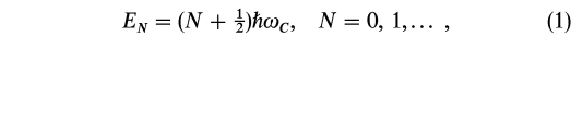
where
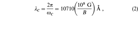
where ωC = eB/mec and λC are the electron cyclotron frequency and wavelength, respectively. The energy levels are equally spaced in frequency and give rise to cyclotron lines at the cyclotron fundamental frequency at the temperatures expected in the photospheres of white dwarfs. The wave functions carry the cylindrical symmetry of the magnetic field.
In contrast, for a bound electron in an H atom dominated by the electrostatic interaction, the energy levels are given by

where n is the Coulomb principal quantum number and ωR is the Rydberg frequency. The wave functions exhibit the spherical symmetry of the electrostatic potential. Each n manifold has a n2 degeneracy. The substates can be labeled by the orbital angular momentum L with quantum number l = 0, 1,...,n - 1, and its projection Lz onto a fixed direction z with quantum number ml = -l, - l + 1,..., 0,...,l - 1,l.
The energy levels of a bound electron in a general magnetic field B are more complex but can be related to the above two cases, though the relationship is strongly nonlinear. We consider the Pashen‐Back limit (B>104 G) appropriate to MWDs, where the spin‐orbital angular momentum interaction is negligible compared to the linear Zeeman effect. The energy levels are then given by the eigenvalues of the Hamiltonian (Garstang 1974)
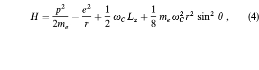
where r is the radial distance of the electron from the proton, θ is the polar angle measured with respect to the field (the z) direction, and p is the linear momentum. The first and second terms represent the kinetic energy and the Coulomb energy, respectively, while the third (the paramagnetic) and fourth (the diamagnetic) terms are introduced by the magnetic interaction. The paramagnetic term is seen to be constant over the entire spectrum and is independent of the degree of excitation of the electron (that is, of r). This term leads to a spread in energy of a given level of

The diamagnetic term, on the other hand, depends strongly on the degree of excitation of the electron, and is of the order of

where a0 is the Bohr radius. This term mixes states of different l, making the problem nonseparable and analytically intractable in the general case.
The separation En,n + 1 in energy between the unperturbed n and n + 1 states is
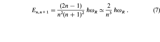
An important reference field can be obtained by comparing the quadratic Zeeman shift of the nth state with the separation En,n + 1 (Schiff & Snyder 1939):
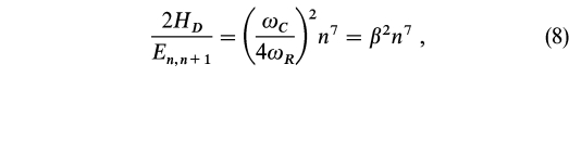
where β = ωC/4ωR = B/4 × 109 G. The n and n + 1 manifolds will intermix due to the quadratic effect if the field exceeds

For β≳1, the level structure of the entire atom (n≥1) will be dominated by the magnetic field. On the other hand, the level n = 6 would have mixed with adjacent levels already at BQ(n = 6) = 9 × 10⁶ G. We note also that HD/HP = n3β/4 so that the quadratic effect quickly dominates as n and/or B increases.
The various regimes have specific characteristics which are seen in WD spectra. In the linear Zeeman regime the diamagnetic term is negligible (β≪1). This is the case for low fields and for low‐lying states. The third term in the Hamiltonian then dominates and results in the removal of the ml degeneracy. Each energy level is simply shifted by an amount 1 / 2 mlℏωC depending on the ml quantum number. Thus the n = 2 level splits into three states (ml = -1, 0, + 1) separated by 1 / 2 ℏωC and the n = 3 level to five states (ml = -2, -1, 0, 1, 2), again separated by 1 / 2 ℏωC, etc.
The effect of the magnetic field on the energy levels which illustrates the linear, and other, regimes to be discussed shortly is shown in Figure 1. The results are based on the calculations of Rosner et al. (1984) (see below).
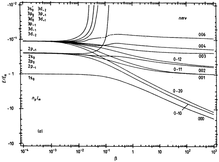
Fig. 1.— The low‐lying energy levels of the hydrogen atom in units of the Rydberg energy as a function of the magnetic field parameter β = B/4.7 × 109 G from Rosner et al. (1984). Copyright Journal of Physics B, reproduced with permission.
Dipole transitions are allowed under the selection rules Δm = 0, -1, + 1 and results in the splitting of what was a single absorption line due to a transition between energy levels of lower principal quantum number nlo and upper principal quantum number nup into a normal Zeeman triplet composed of an unshifted central π component (Δm = 0 transitions), a redshifted σ+ component (Δm = -1 transitions), and a blueshifted σ- component (Δm = +1 transitions). The π component occurs at the zero‐field frequency ω0, while the two satellite σ components occur at ω0 - ωL and ω0 + ωL, where ωL = ωC/2 is the Larmor frequency. The splitting is as in the classical Lorentz theory and is uniform across the frequency spectrum, independently of the value of Δn = nup - nlo (the same for Lyα or Hβ, etc.).
In wavelength units, the splitting between a σ component and the unshifted central π component in the linear regime is
which corresponds to ±10 Å per MG at 5000 Å. It follows that the characteristic pattern of a Zeeman triplet should be readily detectable at the spectral resolutions typically used in white dwarf surveys (∼10 Å) for fields ≳1 MG, provided the splitting is in the linear regime (low fields and low‐lying levels) and the intrinsic broadening of the line due to Doppler and pressure effects does not mask the Zeeman splitting. The ratio of the Zeeman splitting in the linear regime to the Doppler width of a line (δλD = λ 2kT/mec2) is
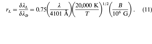
A minimum requirement for the components to be resolved in the linear regime is for rL>1. Thus, we expect to see resolved Zeeman features for fields ≳106 G.
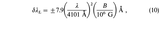
Kemic (1974) extended the Zeeman calculations of hydrogen using perturbation techniques into the first of the diamagnetic regimes where the quadratic term in B begins to play a role in the Hamiltonian though still much smaller than the electrostatic term (β<10-3). In this regime, the l degeneracy is also removed (the "inter l mixing" regime), but n remains a good quantum number[B≪BQ(n)]. The n = 2 energy level now splits into one S (l = 0) state with ml = 0, and three P (l = 1) states with ml = -1, 0, 1; the n = 3 state splits into one S (l = 0) state with ml = 0, three P (l = 1) states with ml = -1, 0, 1, and five D (l = 2) states with ml = -2, -1, 0, 1, 2, etc. (see Fig. 1). Unlike in the linear regime, the energy shifts now depend strongly on the excitation of the electron. The dipole selection rules for permitted transitions are Δl = ± 1 and Δml = 0 and ±1 and result in the splitting of Lyα into three components, Hα into 15 components, etc. In this regime, the π components are also shifted as are the σ components, each by different amounts. The quadratic effect is expected to first manifest itself as an asymmetry in the line profile and a displacement of the centroid of the line from its zero‐field position, and as the field increases the individual components will be seen resolved. For Balmer transitions of the type 2S - nP, the centroid of the line when suitably averaged over the π and σ components is blueshifted due to the quadratic effect by an amount (Preston 1970; Hamada 1971)
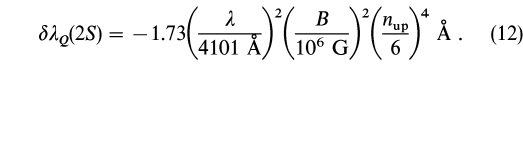
For the 2P–nS and 2P–nD transitions, the shifts are about 40% smaller (Hamada 1971). The shift is strongly dependent on the upper principal quantum number nup in any given series. The quadratic shift becomes comparable with the linear shift for Hδ at fields of 4 × 10⁶ G. The first white dwarfs to be recognized as magnetic by the Zeeman effect in fact exhibited resolvable Zeeman structure in the Balmer series (rL>1) with clear evidence for the quadratic effect (δλQ>δλL) in the higher members of the Balmer series. Examples of such stars will be presented and discussed in § 3.1.
The extension of the Zeeman calculations to still higher fields where the magnetic term first becomes comparable to the Coulomb term in the Hamiltonian (β∼1, the "inter n mixing regime") and then dominates over the Coulomb term (β>1, "the strong field mixing" regime; β≫1, "the Landau" regime) took another 10 years until the work of Rosner et al. (1984), Forster et al. (1984), Henry & O'Connell (1984, 1985), and Wunner et al. (1985). In the first of these high‐field diamagnetic regimes, we have 2ℏωR/n3∼HD, and different n manifolds begin to overlap. The only good quantum numbers are now ml and the z parity πz. In the "strong‐field mixing" regime, we have 2ℏωR/n3∼ℏωC, while in the Landau regime, the magnetic field has an even a stronger influence on the atomic structure dominating over the Coulomb term far into the continuum. Because of the presence of mixed symmetries (spherical from the Coulomb potential and cylindrical from the magnetic field), the complete problem was intractable analytically and was solved essentially by "brute force" using supercomputers. Although the energy level diagram shows no simple structure in the inter n mixing regime, new structure begins to appear in the Landau regime reflecting the fact that at very strong fields the motion of the electron perpendicular to the field is quantized into Landau energy states as for a free electron, while the motion along the field becomes effectively one‐dimensional Coulombic. This structure is expected to manifest itself in spectra at significantly higher fields than found in white dwarfs.
We show in Figure 2 the magnetic field–wavelength (B‐λ) curves for transitions in the hydrogen atom which illustrate these various regimes. We note that the quadratic Zeeman effect is stronger for absorption lines originating from the more excited states (higher values of nlo) and increases with nup for a given nlo becoming relatively more important in the higher members of a given series. In the inter n mixing regime the level structure is very complicated, but at very high fields, a simpler structure appears. Also, some transitions that are forbidden at low fields develop nonnegligible transition probabilities at high fields.
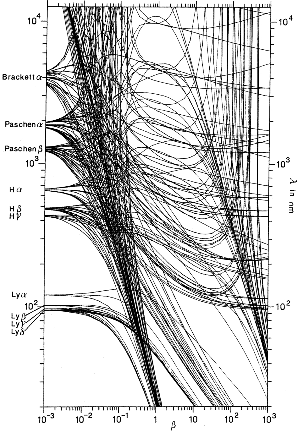
Fig. 2.— Calculations of the Zeeman splitting of hydrogen as a function of the magnetic field parameter β = B/4.7 × 109 G from Wunner (1990). Copyright American Institute of Physics, reproduced with permission.
A striking feature of the B‐λ curves of the σ+ components is the presence of turning points in the vicinity of which the wavelengths of a given transition become nearly stationary. The stationary wavelengths play a crucial role in determining the spectral appearance of high‐field MWDs. Indeed, a standard approach of estimating the magnetic field in a high‐field MWD is to look for features which correspond to turning points in the B‐λ curves since these will suffer the least amount of magnetic field broadening and will have the greatest impact on the surface field averaged spectrum (see § 2.3). The fastest moving components tend usually to be broadened beyond recognition depending on the degree of nonuniformity of the field.
The two‐electron problem is even less tractable analytically and numerically. Until recently, accurate numerical results on the transition energies and probabilities for He i were available only in the low‐field (β≪1; Kemic 1974) regime. Further significant progress was made by Thurner et al. (1993), who presented calculations for several low‐lying triplet states, but these calculations did not cover the intermediate‐field regime of mixed symmetries in fine enough detail to be useful to astrophysicists. More recently, Becken & Schmelcher (1998, 2000) have presented benchmark calculations of the low‐lying singlet and triplet energy levels of He i for the M = 0 and M = -1 even‐ and odd‐z parity states covering all field regimes including the difficult field regime of mixed symmetries. These calculations are currently being extended to cover further M subspaces, and work is also in progress to evaluate transition probabilities between the various levels. It is therefore expected that astrophysicists will soon be in a position to investigate the spectra of helium‐rich MWDs in the same detail as has been possible for the H‐rich MWDs.
Other important developments on atomic structure of relevance to magnetic white dwarfs have been the investigations of the structure of the ground state of the carbon atom (Ivanov & Schmelcher 1999) and of molecular hydrogen (Detmer, Schmelcher, & Cederbaum 1998) at arbitrary fields.
2.2. Zeeman Spectropolarimetry
In the classical theory of Lorentz, an electron in an atom is modeled as a linear harmonic oscillator of frequency ω0. When a magnetic field is introduced, the harmonic oscillator precesses about the magnetic field but is equivalent to a linear oscillator of frequency ω0 along the field (the π component), a circular oscillator of frequency ω0 - ωL which rotates in the same sense as a free electron would in a magnetic field (the r component), and a circular oscillator of frequency ω0 + ωL which rotates in the opposite sense (the l component). The corresponding quantum analogs are the π, σ+, and σ- components, respectively, discussed in the previous section.
The classical model allows the polarization and the intensity of the radiation emitted by each of these oscillators to be easily visualized; for an accelerating electron, the polarization is given simply by the projection of the acceleration vector of the electron in the plane of the sky. The intensity is zero in the direction of the acceleration (Jackson 1963, p. 464). The situation for a π and a σ+ oscillator are illustrated in Figure 3.
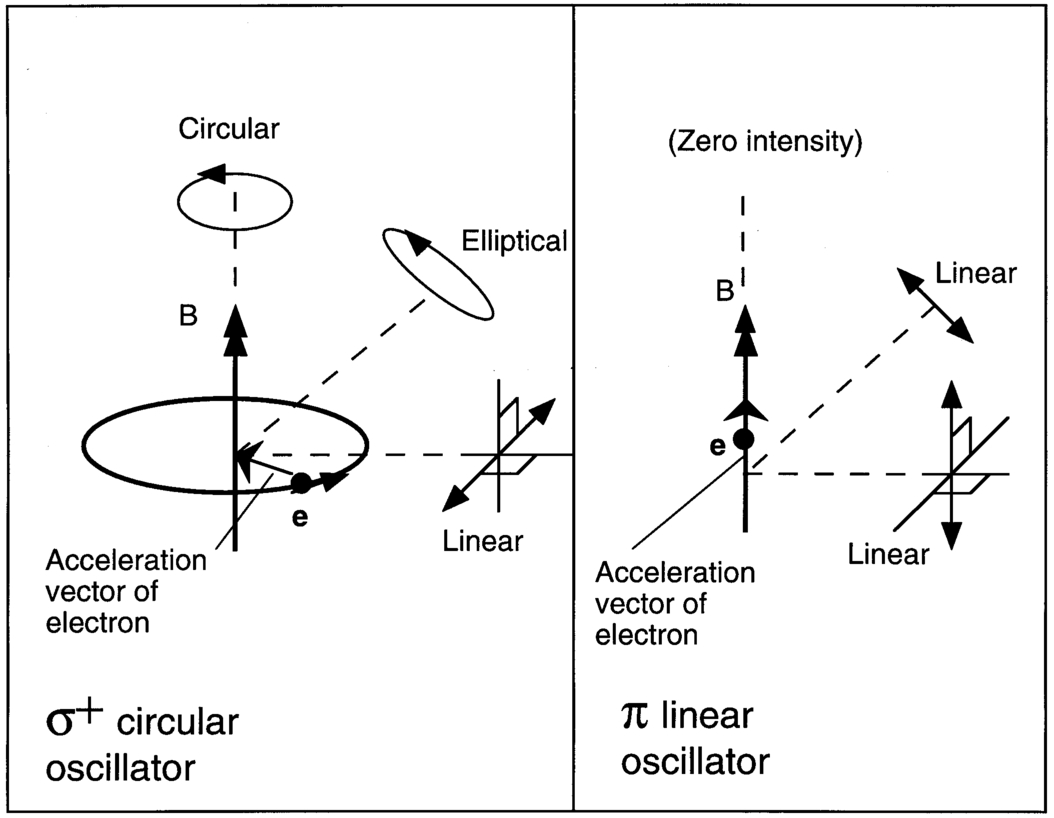
Fig. 3.— Polarization characteristics of the σ+ (circular) and π (linear) oscillators as given by the projection of the acceleration vector of the electron in the plane of the sky. Note that the σ- oscillator has the same characteristics as the σ+ oscillator with the electron moving in the opposite direction.
A σ component will be seen linearly polarized when viewed perpendicular to the line of sight, elliptically polarized at a general viewing angle, and circularly polarized when viewed along the field direction. A π component will be seen linearly polarized at all viewing angles, except that there will be no intensity when viewed along the field. Note that for viewing perpendicular to the field, the σ and π components are linearly polarized in orthogonal directions. Zeeman spectropolarimetry is therefore invaluable for constraining the field, since it carries information not only on field strength but also on field direction.
A powerful method for detecting low‐field magnetic white dwarfs is the measurement of Zeeman splitting through circular polarization induced in the wings of lines. Here one uses the fact that the σ- and σ+ components of a Zeeman triplet have circular polarization of opposite signs, which imparts a net degree of circular polarization in the blue or the red wings of lines even in the low‐field regime when the Zeeman splitting is smaller than the intrinsic pressure width of the line. The presence of a field could therefore be detected even if the spectral resolution is inadequate for the individual Zeeman components to be resolved in the intensity spectrum (§ 2.3). Of course, circular spectropolarimetry will provide information only on the longitudinal component Bl of the field. The transverse component can be similarly constrained by linear spectropolarimetry.
There is another important use of spectropolarimetry. In the case of the AM Her systems when the radiation from the magnetic white dwarf is masked by unpolarized sources of radiation in the binary system (e.g., gas streams), spectropolarimetry is often the only method of detecting Zeeman components and measuring magnetic fields.
2.3. Magnetic Field Broadening and Stark Broadening
In magnetic white dwarfs, we expect the field strength and direction to vary over the stellar surface. For example, in a centered dipole distribution the field strength varies by a factor of 2 from the pole to the equator. For a dipole that is displaced from the center along the dipole axis by a fractional d of the stellar radius, the ratio of the field strengths at the opposite poles is (1 + d)3/(1 - d)3 and could take extreme values. Since the line and continuum opacities are strong functions of field strength and orientation, so are the solutions to the polarized radiative transfer equations which determine the properties of the emergent radiation field. In practice, individual model atmospheres have, therefore, to be constructed on selected points on the visible stellar surface taking into account field variations and the resulting Stokes intensities suitably summed to obtain a theoretical spectrum (Martin & Wickramasinghe 1979a).
The positions, intensities and polarization of the Zeeman components of a line are usually strongly dependent on magnetic field strength (except for the "stationary" components) as was shown in § 2.1. A component would therefore, be broadened simply by field spread over the visible stellar disk. This is known as magnetic field broadening. The width imparted to such a component due to a spread δB in field in the linear Zeeman regime is δνB∼ 1 / 2 νC(δB/B) or δλB∼ 1 / 2(λ2/λC)(δB/B) The ratio of the widths due to field spread and Doppler broadening is
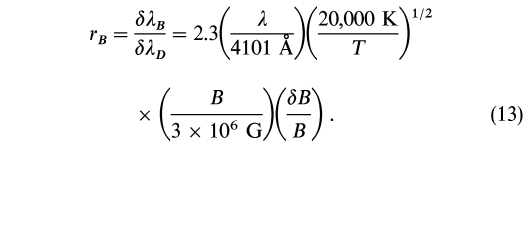
Clearly for δB∼0.3B (e.g., for a centered dipole) the width due to field spread exceeds the thermal width ∼10 Å (i.e., rB>1) for fields above ∼3 × 10⁶ G. Below this value, the line cores of the Zeeman triplet will be broadened by the Doppler (and Stark) effects.
There is at present no Stark broadening theory for hydrogen that could generally be applied to the magnetic WDs, but some calculations are available of the Stark effect for field strengths appropriate to the Ap stars which may be applicable to low‐field WDs. In the presence of an electric field, a degenerate energy level n of an H atom is split into distinct subcomponents due to the linear Stark effect. The maximum separation between the Stark components for a level n is given by

where  is the microelectric field (Bethe & Salpeter 1957, p. 231). If we use the characteristic electric field 0 = 2.61eN2/3 corresponding to the average separation between ions, the ratio of the Stark width of a level n to the width due to Zeeman spitting is given by
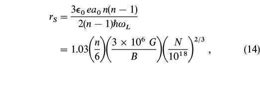
where N is the ion density. If rS≫1 for the upper level of a given transition, and the splitting is in the linear regime (δλQ<δλL), we expect the effect of the magnetic field to be restricted to the line core which will be composed of a Zeeman triplet, that will be resolved if rL>1. On the other hand, the far wings are determined by the Stark effect at fields much larger than 0 and will have profiles which are independent of the magnetic field. Under these circumstances, Stark broadening theory (with B = 0) can be used to determine gravities using the wings of lines. Our estimates indicate that for the densities expected in a WD atmosphere (N∼1018 cm−3), this theory can be used in the wings of lines for Hα‐Hδ at fields of ≲ 2 × 10⁶ G.
Mathys (1984) has presented some calculations of the combined Stark and Doppler profiles of Zeeman‐split H lines in the low‐field linear Zeeman regime using the unified classical path theory, with the ions treated in the quasi‐static approximation which supports the above contention. His calculations which allow for polarization and the vector character of the microelectric fields show that although the Stark profile becomes a function also of the viewing angle with respect to the magnetic field direction, the line wings are independent of both the field strength and viewing angle in the limits discussed above.
The regime rS≪1 is more difficult to treat even in the linear Zeeman regime. Furthermore, although equation (14) indicates that the Stark width will always dominate over the (linear) Zeeman width in the higher members of a given series (rS∝B-1n) at fixed B, in practice, the quadratic Zeeman effect will take over at high fields and high n[rS(quad)∝B-2n-2], resulting in the splitting of such a line into many subcomponents. There is no adequate theory for handling Stark broadening in these regimes, but some attempts have been made to investigate this problem.
Friedrich, König, & Schweizer (1996a) considered the special case of an electric field oriented parallel to a magnetic field. They assumed that the magnetic field has no effect on the microfield distribution and neglected the curvature of the motion of charged particles. These calculations, which are in the difficult regime discussed above where the quadratic Zeeman effect is important but the individual components still overlap, have shown very large deviations from observations.
At still higher fields, when the Zeeman components separate, Friedrich et al. (1994) calculated that the Stark width was reduced by a factor of ∼100 to ∼0.2 Å for the 2s0–3p0 transition at its stationary wavelength (B∼2 × 10⁸ G). At these fields, theory suggests that the Stark effect will be of secondary importance compared to Doppler broadening and magnetic field broadening. Indeed, the empirical evidence is that when the field is strong enough for l degeneracy to be removed, Stark broadening is reduced by a factor of ∼10 or more below the zero‐field values for individual components (Martin & Wickramasinghe 1984; Putney & Jordan 1995).
At very low fields, when the Zeeman effect is in the very core of the line and the wings can be calculated using standard (zero magnetic field) Stark broadening theory, gravities can be determined by model atmosphere calculations almost independently of field structure. Attempts at estimating gravities and masses from line profiles have therefore been restricted to a few of the very low field magnetic white dwarfs where Zeeman splitting is small and existing Stark broadening theories (at zero magnetic field) could be used to calculate the line wings. For higher field stars, the best bet for determining gravities may be to use the "stationary" components. The line profiles of these components will be determined mainly by Doppler (and to a lesser extent Stark) broadening, but magnetic field broadening will still play some role.
The very strong dependence of the spectral appearance on field spread and geometry at intermediate and high fields has enabled magnetic field geometry to be investigated in significant detail in these stars, even in the absence of a suitable Stark broadening theory. The approach that has been adopted up to the present time has been to model the lines by a Voigt profile and to adjust the damping width of individual components below the Stark values predicted by the zero‐field impact and statistical broadening theories (Martin & Wickramasinghe 1984; Putney & Jordan 1995). The rapidly moving components will provide the most information on field structure. The extent to which field structure can be constrained depends on the nature of the data that is being analyzed. Clearly, an intensity spectrum alone will provide fewer constraints than an intensity and polarization (linear and circular) spectrum. The best constrained models are those which are based on observations at different rotational phases, but such data are available for only a few stars. For most magnetic white dwarfs the data to be modeled are restricted to an intensity (and sometimes a polarization) spectrum corresponding to a single viewing (magnetic) phase. In such cases the models are not strongly constrained, although some field structures can be eliminated even in these case.
The modeling procedure generally adopted is to progress from the simplest field structure, namely, that of a centered dipole, to more complex field structures, such as offset dipoles or combinations of higher order multipoles, as required by observations. The most commonly used models are the offset dipoles. These are specified by the polar field strength Bd of the centered dipole prior to displacement and the fractional radial displacements (ax,ay,az) of the dipole from the center of the star, where z is in the direction of the dipole axis (Achilleos & Wickramasinghe 1989; Putney & Jordan 1995). Another approach has been to expand the field in multipolar components and use a best‐fit criterium (e.g., least squares or maximum entropy) to obtain expansion coefficients (Donati et al. 1994; Burleigh, Jordan, & Schweizer 1999).
2.4. Continuum Polarization
While Zeeman identifications provide the most direct and accurate method for measuring magnetic fields, the existence of fields and an estimate of field strength can also be obtained from continuum polarization as originally proposed by Kemp.
Elementary absorption (and scattering) processes in the continuum involving electrons are affected by the presence of a magnetic field and result in field and polarization dependent absorption (and scattering) cross sections (magnetic dichroism). In addition, electromagnetic waves propagate with different phase velocities depending on the polarization state leading to "propagation" or "Faraday" effects (magnetic birefringence). In the presence of a magnetic field, the polarization characteristics of a typical absorption (or emission) process range from being circular along the field, to elliptical at a general angle to the field, to linear perpendicular to the field, but there could be a conversion of one sort of polarization to another during radiative transfer due to Faraday effects. The degree and type of polarization of the radiation which emerges from an atmosphere will depend on the sources of magnetic dichroism, magnetic birefringence, and radiative transfer effects through the atmosphere.
Although the wavelength dependence of polarization could be quite complicated, the ratio of linear to circular polarization is expected to have a simpler behavior. For a plane‐parallel atmosphere in which the eigenmodes of propagation are those of a fully ionized plasma and Faraday terms dominate over absorption terms, this ratio is given by Martin & Wickramasinghe (1982) (see also § 5.4):
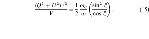
where ξ is the angle between the line of sight and the magnetic field vector which is assumed to be oriented perpendicular to the atmosphere. For frequencies below the cyclotron resonance (in the optical region for field strengths greater than 2 × 10⁸ G) the polarization will be mainly linear except for a range of viewing angles close to the field direction, while for frequencies above the cyclotron resonance (in the optical region for field strengths less than 2 × 10⁸ G) the polarization will be mainly circular except for a range of viewing angles almost perpendicular to the field direction.
For the wavelength dependence of the continuum emission, away from bound‐free edges, and for ωC/ω≪1, we expect
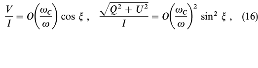
for a plane‐parallel atmosphere for a variety of processes (§ 5.4). Of course, what is observed is an average over the visible stellar disk and will be affected by field structure. For instance, for a centered dipole, only circular polarization will be seen for pole‐on viewing and only linear polarization for equator‐on viewing (Martin & Wickramasinghe 1979a).
Current models predict that high‐field (≳100 MG) white dwarfs will show comparable degrees of linear and circular polarization (∼10%–30%) in the optical band, but the uncertainties in such calculations are large due to our lack of detailed knowledge of opacities (§ 5.3). Empirically, high‐field white dwarfs tend to show (Q2 + U2)1/2/V∼0.2–0.6 in the optical with the exception of GD 229 for which (Q2 + U2)1/2/V∼8 (see § 5.4.1).
2.5. Cyclotron Spectroscopy of Isolated MWDs
Classically, free electrons in a magnetic field will give rise to radiation at the cyclotron fundamental and its harmonics depending on the temperature of the plasma (Bekefei 1966). At low temperatures most of the power will be at the cyclotron fundamental, and therefore it was expected that some MWDs will show a spectroscopic signature at the wavelength of the cyclotron fundamental which occurs in the optical‐UV region at high fields. There has so far been no convincing direct evidence for such a feature in the intensity spectrum of an isolated MWD. Magnetic broadening (see § 2.3) is expected to broaden this feature to the limit of undetectability for most field geometries (Martin & Wickramasinghe 1979b). However, there may be indirect evidence that the cyclotron resonance occurs in the optical region in some stars through the observed rotation by 90° of the polarization angle with wavelength (§ 5.4.1).
Although there has been no convincing identification of a cyclotron feature in the intensity spectrum of an isolated MWD, resolvable cyclotron lines at the fundamental and its overtones have been detected from high‐temperature (≳10 keV) accretion shocks on magnetic white dwarfs in the AM Herculis binaries (§ 6.2.2).
3. OBSERVATIONS OF ISOLATED MAGNETIC WHITE DWARFS
3.1. Low‐Field Magnetic White Dwarfs
We illustrate the circular spectropolarimetric technique for discovering magnetic white dwarfs in Figure 4. LP 907‐037 (=WD 1350−090, B∼85 KG) is the first of the low‐field MWDs to be identified through Zeeman circular spectropolarimetry (Schmidt & Smith 1994). Here Hβ and Hα are both seen as single unsplit lines in the intensity spectrum so that the Zeeman splitting is smaller than the intrinsic Doppler width (rL<1). Futhermore, magnetic field broadening is expected to be unimportant (rB<1). However, the lines separate out into clearly resolved σ+ and σ- components in the circular polarization spectrum.
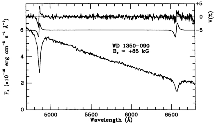
Fig. 4.— Intensity and circular polarization spectra of the low‐field (B = 85 KG) white dwarf LP 907‐037 (WD 1350−090). The σ- and σ+ components are seen in left‐ and right‐circularly polarized light but not in the intensity spectrum. A model polarization spectrum is also shown, offset by 5% in polarization for clarity (Schmidt & Smith 1994). Copyright Astrophysical Journal, reproduced with permission.
One of the new results to have emerged in recent years has been the evidence for high gravities in low‐field stars where the Zeeman splitting in the lower members of the Balmer series is restricted to the line cores. The spectra of two such stars, PG 1658+441 (Bd = 3.5 MG; Schmidt et al. 1992a) and 1RXS J0823.6−2525 (Bd = 3.5 MG; Ferrario, Vennes, & Wickramasinghe 1998), with model fits based on zero‐field Stark broadening theory and dipole field distributions, are shown in Figure 5. The broad wings, indicative of high gravities can be clearly seen in the data. From the discussion of § 2.3, the zero‐field Stark broadening theory should be adequate to describe Hβ and Hγ, but quadratic shifts and magnetic field broadening will very quickly dominate in the higher Balmer lines. Since the weighting in the model fits is mainly from the lower members of the Balmer series, the mass estimates are expected to be reasonably secure. The masses deduced are 1.2 M⊙ for 1RXS J0823.6−2525 and 1.31 M⊙ for PG 1658+441, but the actual uncertainties may be somewhat larger than indicated.
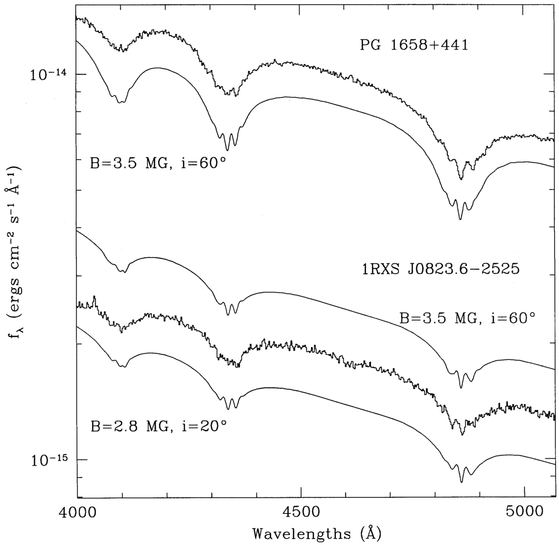
Fig. 5.— Intensity spectra of the low‐field ultramassive MWDs PG 1658+441 (Schmidt et al. 1992a) and 1RXS J0823.6−2525 (Ferrario et al. 1998) showing strongly Stark‐broadened Balmer lines. The underlying model for PG 1658+441 assumes Teff = 30,000 K and log g = 9.36, and the model for 1RXS J0823.6−2525 assumes Teff = 43,200 K and log g = 9.02. Copyright Monthly Notices of the Royal Astronomical Society, reproduced with permission.
The spectra of intermediate‐ and high‐field MWDs are generally very sensitive to field structure, and as a consequence, spectroscopic observations, even at a single rotational phase, can be used to place some constraints on field structure. We show in Figure 6 a series of centered and off‐centered dipolar models compared with the observations of Downes & Margon (1983) of the white dwarf KPD 0253+5052 (Achilleos & Wickramasinghe 1989) to illustrate the modeling procedure. For a given offset, the dipole strength Bd is chosen to provide the correct mean field to match the observed positions of the Zeeman components. In this field regime, the profiles of the Zeeman components are dominated by magnetic field broadening, and the faster moving σ components, in particular, are seen to be strongly field geometry dependent. As the dipole is moved toward the observer, the field spread across the visible hemisphere increases, and these features are more spread out in wavelength. We see that the off‐centered dipole with az = 0.2 clearly provides a better fit to the profile of the σ- component of Hβ near 4600 Å. The possibility of a centered dipole model can be dismissed for this star even on the basis of a single spectrum. Similar analyses have been carried out for other stars by a number of investigators (e.g., Putney & Jordan 1995) and form the basis for the field estimates in Table 1. The field estimates are generally based on offset dipole models, often on a single spectrum, unless otherwise stated.
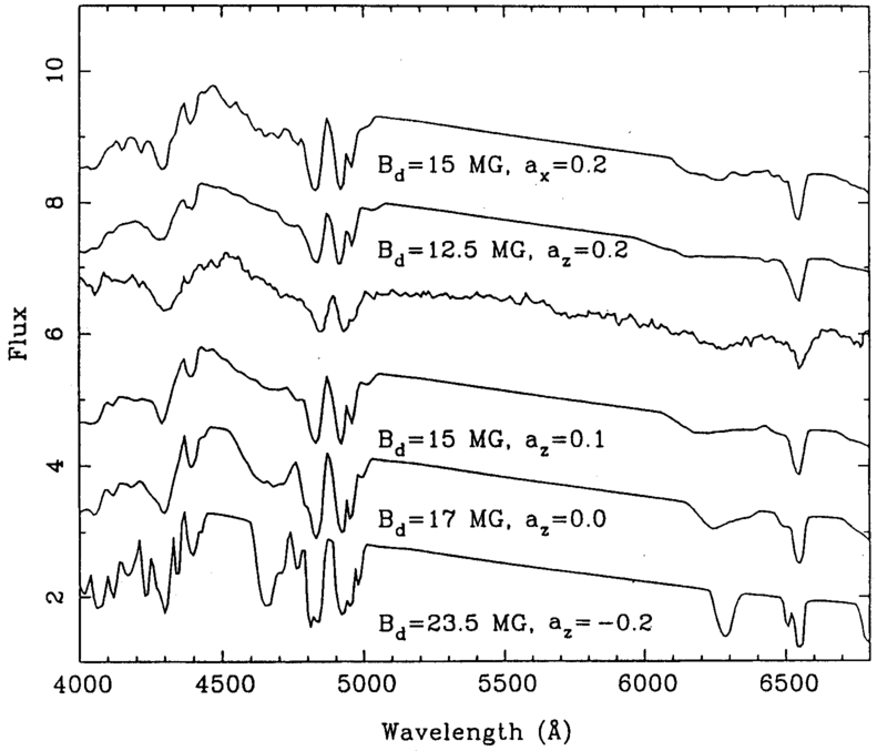
Fig. 6.— Observations of KPD 0253+5052 from Downes & Margon (1983) (third spectrum from the top) compared with best‐fit centered dipole and decentered dipole models (i = 20°). The best‐fit model is from Achilleos & Wickramasinghe (1989) and has a field strength Bd = 12.5 MG with the dipole offset toward the observer (az = 0.2). Copyright Monthly Notices of the Royal Astronomical Society, reproduced with permission.
 |
 |
3.1.1. GD 356: A Unique Emission‐Line Magnetic White Dwarf
Observations of the unique magnetic white dwarf GD 356 show resolved Zeeman triplets of Hα and Hβ in emission with distinctive circular polarization properties. The detailed modeling of the spectropolarimetric observations points to the existence of a latitudinally extended region covering a tenth of the stellar surface over which the stellar atmosphere has an inverted temperature distribution at low optical depths and produces emission lines (Ferrario et al. 1997b). The narrow circular polarization features which are observed near the central π components of the emission lines (Fig. 7) are attributed to magneto‐optical (Faraday) effects (§ 5.1.1) in regions of the photosphere which gives rise to an underlying (but mainly masked) absorption spectrum.
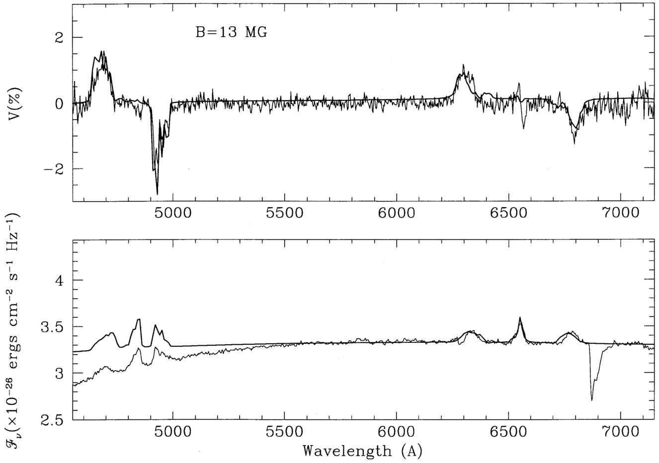
Fig. 7.— Intensity and polarization spectra (bottom and top panels, respectively) of the unique emission line white dwarf GD 356 superimposed on the calculated spectra. Magneto‐optical effects from regions producing photospheric absorption appear to be responsible for the narrow circular polarization features which are observed near the π component of the emission lines. Copyright Monthly Notices of the Royal Astronomical Society, reproduced with permission.
The reasons for the temperature inversion in GD 356 remain a mystery. Radio observations obtained at the Very Large Array at 8439.9 MHz and 4860.1 MHz, yielded a null result, thus failing to provide evidence for magnetic activity through the detection of a corona. IR observations to search for a low‐mass stellar companion as a possible source of matter for accretion also yielded null results. One intriguing possibility proposed by Li, Ferrario, & Wickramasinghe (1998) is that GD 356 may have a conducting planetary core in close orbit. Electrical currents may then flow between the white dwarf and the planet and result in the heating of its upper atmosphere through ohmic dissipation.
3.2. White Dwarfs with Fields in the Range 80–1000 MG
3.2.1. Grw +70°8047
Perhaps the single most important result on MWDs in the 1980s was the demonstration that the spectrum of the star Grw +70°8247, which had defied explanation for nearly 50 years, could be interpreted in terms Zeeman‐shifted H lines in a magnetic field of 100–400 MG (Angel, Hintzen, & Landstreet 1985; Wickramasinghe & Ferrario 1988; Jordan 1989; Wunner 1990; Jordan 1992a).
A comparison between the theoretical B‐λ curves based on the Zeeman calculations of Forster et al. (1984) and the observations of Grw +70°8247 is shown in Figure 8. All the strong features in the spectrum correspond to stationary points in the B‐λ curves of transitions originating from the 2s state (mainly Hα and Hβ components) and some transitions originating from the 3d state in the field range ∼100–400 MG (§ 2.1). Note that the observed features are intrinsically narrow due to the reduction in Stark broadening at high fields resulting from the removal of l degeneracy (§ 2.3). Synthetic spectra for a series of centered dipole models of varying polar field strength Bp (Wickramasinghe & Ferrario 1988) are compared with the data of Angel et al. (1985) in Figure 9. The best overall agreement occurs when Bp = 320 MG.
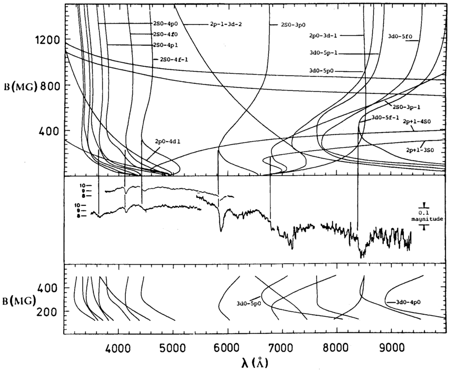
Fig. 8.— Observations of Grw +70°8247 obtained by Angel et al. (1985) (center panel) compared with the field‐wavelength dependence of Zeeman components of hydrogen based on calculations by Forster et al. (1984) and Rosner et al. (1984) (upper panel) and Henry & O'Connell (1984, 1985) (lower panel). Copyright Astrophysical Journal, reproduced with permission.
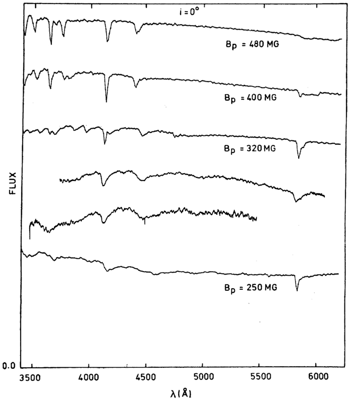
Fig. 9.— Observations of Grw +70°8247 obtained by Angel et al. (1985) and theoretical spectra (Fν vs. λ) of centered dipole models with viewing angle i = 0° for different polar field strengths (Wickramasinghe & Ferrario 1988). The best‐fit model has Bp = 320 MG. Copyright Astrophysical Journal, reproduced with permission.
Although the overall agreement is good, attempts at very detailed comparisons of profiles of individual stationary transitions (e.g., for 2s0–3p0 and 2s0–4f0) with theory have not been particularly successful (Friedrich et al. 1994). This is perhaps not surprising since the Stark broadening theory at high fields is still at a rudimentary stage, and field structure may play some role in determining the profiles of even the stationary components.
The Zeeman effect can also be seen in the IUE UV spectrum where the Lyα σ+ component is seen shifted from its zero‐field position to 1347 Å in the red wing of the very strong π component. The data also show a broad shallow depression at 2500 Å attributed to the faster blueward moving nonstationary components of the Balmer lines (Angel et al. 1985; Wickramasinghe & Ferrario 1988). We present in Figure 10 a comparison between observations (Greenstein & Oke 1982) and theoretical calculations by Jordan (1992a) in this wavelength region.
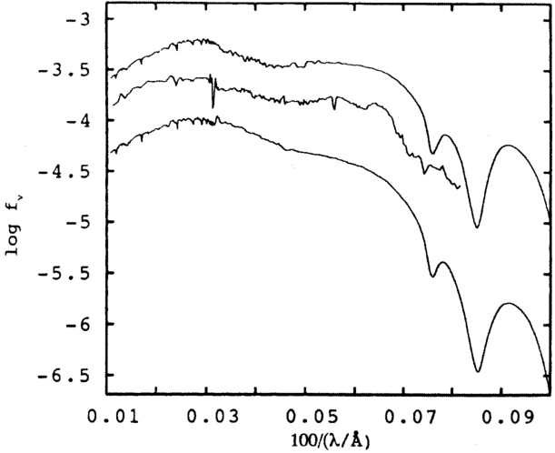
Fig. 10.— The UV spectrum of Grw +70°8247 taken from Greenstein & Oke (1982) (middle spectrum) compared with two centered dipole models with Te = 16,000 K (top spectrum) and Te = 14,000 K (bottom spectrum) and Bp = 320 MG from Jordan (1992a). The model shows the central π and satellite σ+ and σ- components of Lyα. The narrow feature centered at 100/λ = 0.074 is attributed to the 1s0–2p-1 σ- component. We note also the broad depression centered at 100/λ = 0.04 due to the fast blueward‐moving higher Balmer lines. Copyright Astronomy and Astrophysics, reproduced with permission.
Grw +70°8247 has been extensively observed in polarized light. The broadband linear and circular polarization observations from West (1989) combined with optical spectropolarimetry of Landstreet & Angel (1975) is shown in Figure 11. The data shows a rotation in the polarization angle by 90° at ∼5500 Å, the origin of which will be discussed in § 5.4.1. The general characteristics of the polarization curves have remained invariant for ∼25 yr and indicate that this star is a very slow rotator.
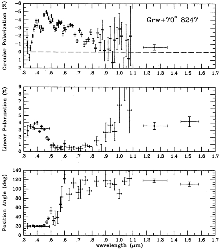
Fig. 11.— IR polarization measurements of Grw +70°8247 from West (1989) combined with the optical spectropolarimetry of Landstreet & Angel (1975). Note the flip by 90° in the position angle as the wavelength increases above the critical wavelength λcrit∼5500 Å. Copyright Astrophysical Journal, reproduced with permission.
3.2.2. GD 229
The very recent calculations of the Zeeman spectrum of He i in strong fields by Becken & Schmelcher (1998) have solved one of the major remaining mysteries in the interpretation of the spectra of magnetic white dwarfs.
GD 229 was discovered to be strongly linearly and circularly polarized by Swedlund et al. (1974) and Landstreet & Angel (1974) and has been studied extensively by a number of investigators (e.g., Liebert 1976; Green & Liebert 1981; Schmidt et al. 1990, 1996a). HST spectropolarimetric observations obtained by Schmidt et al. (1996a) failed to reveal any evidence of Lyα, indicating an H‐poor atmosphere.
We show in Figure 12 and Figure 13 a comparison of the optical and HST UV observations by Schmidt et al. (1996a) with the new calculations of the transition wavelengths of He i in strong magnetic fields. The line lists are presently only complete for transitions between the low‐lying energy levels of the M = 0 and M = -1 even and odd parity states. The B‐λ curves have been calculated from the energy levels presented by Becken et al. (1999) and Becken & Schmelcher (2000) and represent spline fits to the data. The transitions originating from the singlet and triplet states show stationary wavelengths that are in close agreement with some of the features seen in GD 229 in the field range 300–700 MG as noted by Jordan et al. (1998). We note, in particular, the large number of transitions originating from the 23S and the 21S levels with turning points in the wave band 2000–3500 Å where a structured absorption band is seen in the observations. The agreement between the calculations and the observed structure is excellent for most features, and the remaining discrepancies are likely to be attributable to the sparseness of the theoretical grid on which the B‐λ curves are based.
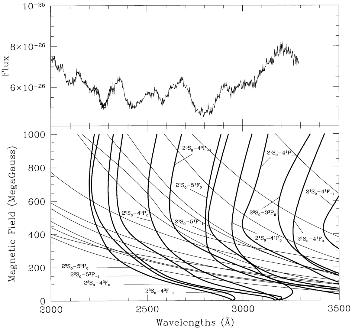
Fig. 12.— The UV spectrum of GD 229 Schmidt et al. (1996a) is compared with B‐λ curves of a selected set of He i transitions between the M = 0 and M = -1 subspaces recently calculated by Becken et al. (1999; Becken & Schmelcher (2000). The comparison includes all stationary transitions at high fields as in Jordan et al. (1998), a new stationary transition, and a subset of transitions which are nonstationary at high fields but which are known to have an impact in the interpretation of lower field He MWDs.
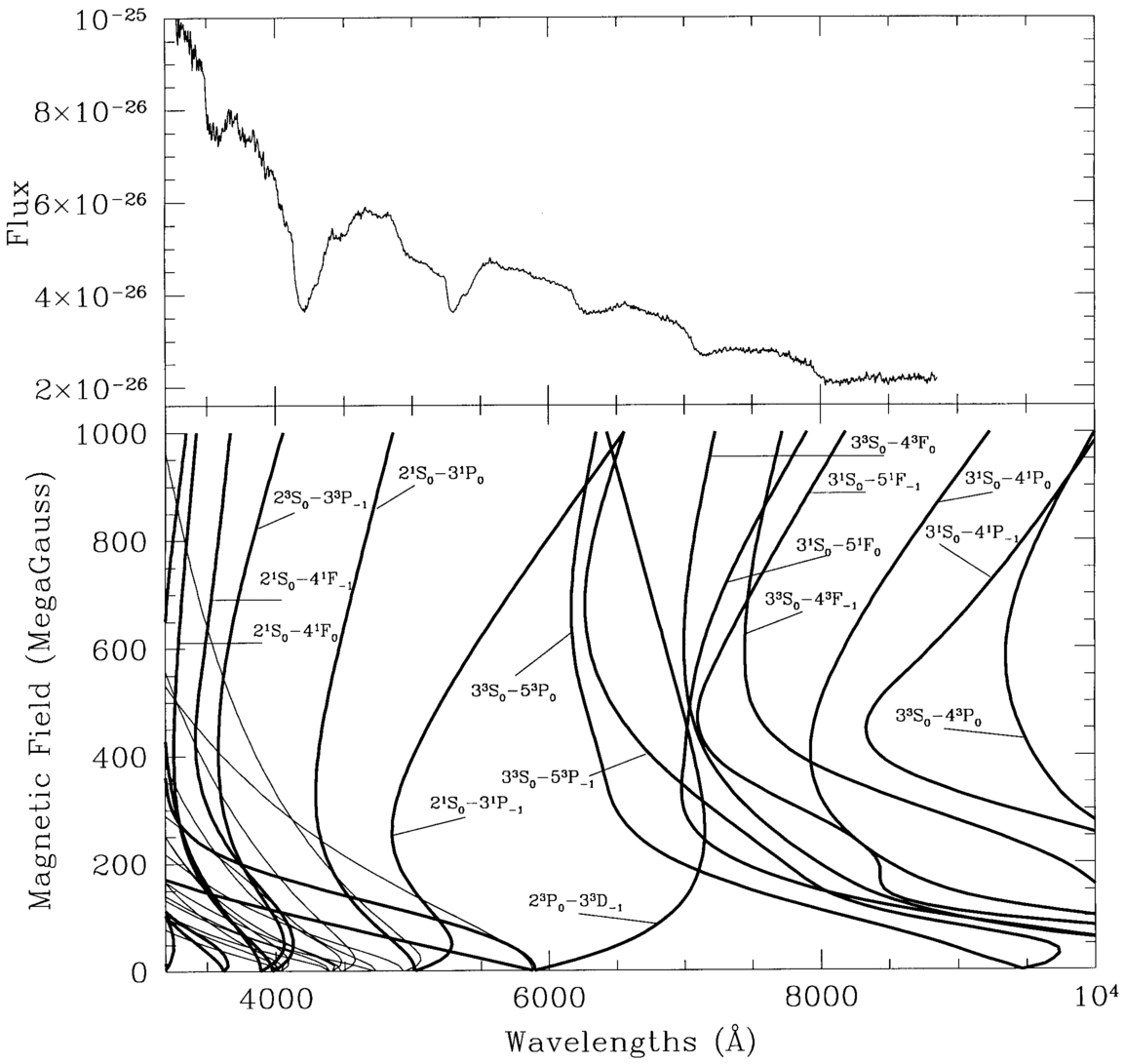
The agreement between theory and the observed features in the optical band is also striking. Convincing identifications are possible for the three features centered at 8000, 7000, and 6200 Å with transitions originating from the 23P and 31S and 33S states. The latest calculations of Becken & Schmelcher (2000) have shown that the 23P0–33D-1 transition (a component of the strong He i λ5876 line) has a stationary point (a broad wavelength maximum) at 7143 Å at a field of 200–400 MG. This is likely to be a major contributor to the observed band at ∼7000 Å. However, there are many other components arising from the 3S levels which also make a contribution to this feature.
The large widths and depths of the stronger features at 4100 Å and 5280 Å are unusual for high‐field MWDs, and these features must again be blends of many individual overlapping components. The main contributors to these features are presently unidentified. These are likely to be the π and σ components involving the M = -2, + 1, + 2 subspaces (e.g., the 23P-1–43D-2, 23P1–43D2 transitions), which still remain to be calculated.
3.2.3. The Magnetic DQ Stars
The atmospheres of nonmagnetic white dwarfs tend to be monoelemental consisting of either essentially pure hydrogen or pure helium, and a similar situation pertains in the magnetic white dwarfs. The white dwarfs dominated by He in their atmospheres usually exhibit atomic helium lines (the DB and DO stars), but the cooler stars show molecular bands of C2 and CH (the DQ stars).
There are also magnetic analogs to stars of spectral type DQ. The best known example is LP 790‐29 (=LHS 2293) (Liebert et al. 1978; Wickramasinghe & Bessell 1979) which shows distorted Swan bands of C2 with the centroids shifted from the zero‐field positions by about ∼10–70 Å by the quadratic Zeeman effect. The spectrum of this star has been modeled by Bues (1999) (see Fig. 14) assuming an H‐deficient atmosphere with He∶C = 1400 with a field of 50 MG. Another star, G99‐37, shows, in addition to C2, Zeeman‐shifted CH bands in the linear regime at a mean field of 3 MG (Angel et al. 1975). A recent addition to the DQ class is the strongly polarized cool white dwarf LHS 2229 (Schmidt et al. 1999a). The broad similarities to LP 790‐29 are apparent, as shown in Figure 15. The differences in the band shapes of the band profiles may be due to differences in field structure. However, the features E and F do not appear to be due to C2, and a DQ "peculiar" classification has been proposed with the suggestion that other molecules such as C2H may be playing a role.
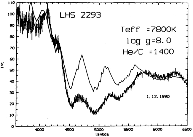
Fig. 14.— Normalized flux of the best‐fitting model atmosphere compared to observations of LP 790‐29 (=LHS 2293). The magnetic field strength is 50 MG (Bues 1999). Copyright Astronomical Society of the Pacific, reproduced with permission.
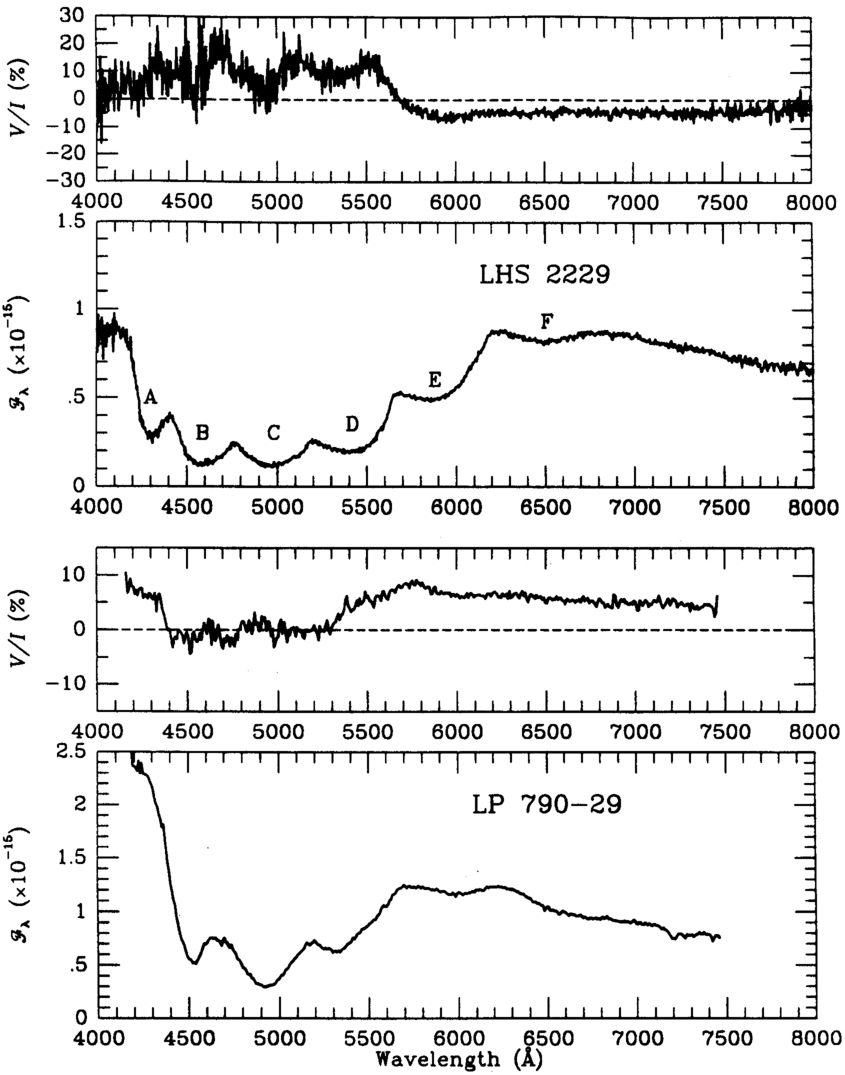
Fig. 15.— Flux and circular polarization spectra of two cool white dwarfs (LHS 2229 and LP 790‐29) with strong molecular features (Schmidt et al. 1999a). Copyright Astrophysical Journal, reproduced with permission.
3.3. Rotating Isolated Magnetic White Dwarfs
Rotation in MWDs was first discovered through the measurement of periodic variations in the broadband circular polarization of G195−19 (Angel & Landstreet 1971). Several other stars have since been discovered to exhibit polarization and/or spectrum variations with rotational phase. The variations are caused by the different aspects of the surface field distribution that is presented to the observer as the star rotates and can be interpreted in terms of a variant of the oblique dipole rotator model (a dipolar field with the dipole axis inclined to the rotation axis) first introduced by Stibbs (1950) to explain the observed reversing field of the magnetic variable Ap star HD 125248. The main difference is that in the MWDs (and also in some Ap and Bp stars) the field structures tend in general to be more complicated than dipolar.
Phase‐dependent observations of rotating MWDs have been used to place strong constraints on field structure using an oblique magnetic rotator model. These studies show that some magnetic white dwarfs exhibit extreme field structures which cannot be modeled by centered or offset dipoles and imply the presence of dominant high‐order multipole components.
3.3.1. EUVE J0317−855: An Ultramassive High‐Field Magnetic White Dwarf
EUVE J0317−855 was discovered to be a magnetic white dwarf with an optical photometric (Barstow et al. 1995) and polarimetric (Ferrario et al. 1997a) period of 725 s. The optical spectrum was modeled by an offset dipole with Bd = 450 MG and az = -0.35 (Ferrario et al. 1997a), as shown in Figure 16, and the same authors also proposed that the splitting of the phase‐averaged Lyα line into a doublet may also be due to the presence of two poles of different field strengths. Subsequently, Burleigh et al. (1999) obtained phase‐resolved HST spectra in the UV which confirmed that the σ+ Lyα line splits into a doublet at some phases and modeled these variations with a surface field distribution in which the field strength varies between 180 and 800 MG, generally consistent with the picture obtained from the optical modeling. The results from this analysis are shown in Figure 17.
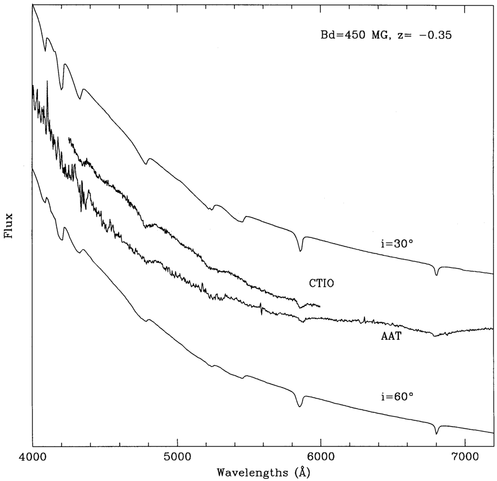
Fig. 16.— CTIO and AAT spectra of the magnetic white dwarf EUVE J0317−855 compared with a calculated spectrum corresponding to a dipolar magnetic field strength of 450 MG and an offset of 35% of the stellar radius along the dipole axis away from the observer (Ferrario et al. 1997a). The models correspond to different viewing angles as marked. Copyright Monthly Notices of the Royal Astronomical Society, reproduced with permission.
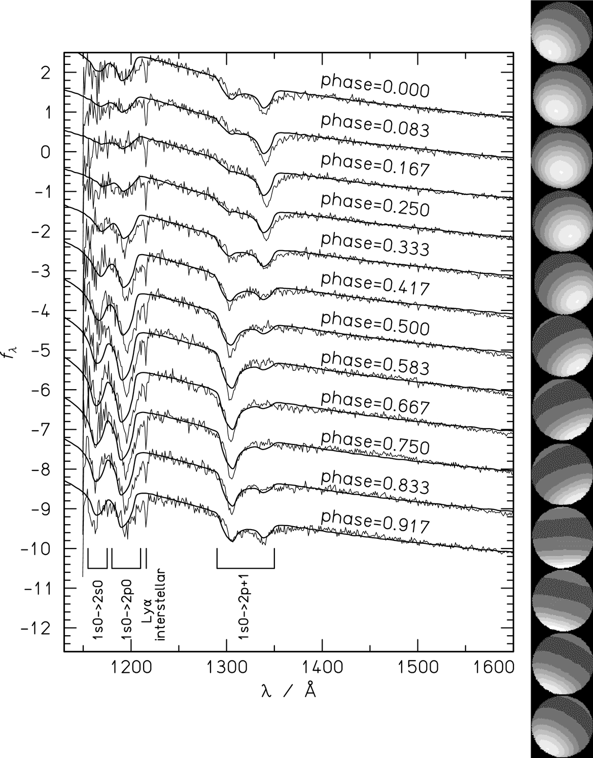
Fig. 17.— HST‐FOS far UV spectra of EUVE J0317−855 for 12 phases together with theoretical model fits from Burleigh et al. (1999). The steps in gray scale correspond to steps of 100 MG. The lowest field is 170 MG (darkest gray), and the highest 800 MG. Copyright Astrophysical Journal, reproduced with permission.
Ferrario et al. (1997a) have shown that the oblique rotator model can also explain the observed amplitude of the photometric variations over a period of 725 s in the optical, simply through the field dependence of the continuum opacity (magnetic dichroism) and the changes in the field distribution over the visible stellar surface as the star rotates.
The proximity of EUVE J0317−855 to the DA white dwarf LB 9802 prompted Barstow et al. (1995) to propose that these stars were physically associated. With this assumption, the mass of the MWD is found to be within a few percent of the Chandrasekhar limit. Ferrario et al. (1997a) proposed that EUVE J0317−855 did not evolve as a single star, but was itself the result of a DD merger. This conclusion was supported by their study of the companion star LB 9802 which uncovered an age paradox: the more massive of the pair, EUVE J0317−855, with M = 1.35 M⊙ (or log g = 9.5), appears also to be the younger!
3.3.2. PG 1015+014: An MWD Spectrum with Hα Fully Resolved
The phase‐averaged spectrum of the rotating (P = 99 minutes) magnetic white dwarf PG 1015+014, which has a field marginally lower than that of Grw +70°8247, is shown in Figure 18 (Wickramasinghe & Cropper 1988). The optical spectrum shows an unusual forest of Hα components (both stationary and fast moving) which are all individually resolved and some of Hβ components shifted by up to 1000 Å from their zero‐field positions. Magnetic field broadening plays a critical role in determining the appearance of the spectrum, but none of the field structures that have so far been considered provides an adequate representation even of the phase‐averaged data. The strong impact that the faster moving components have on the spectrum suggests that the field is quite uniform, perhaps dominated by higher order multipoles. The best‐fit centered dipole model has a polar field strength Bd = 120 MG viewed near equator‐on.
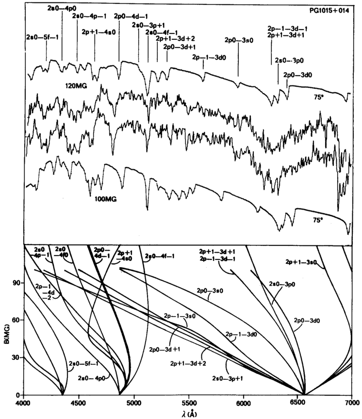
Fig. 18.— The magnetic field B and wavelength λ curves for Hα, Hβ and Hγ transitions from Wunner et al. (1985) and Kemic (1974). Top: model fluxes (Fν vs. λ) compared with the observed spectra of PG 1015+014 at phase 0.75 (upper spectrum) and phase 0.0 (lower spectrum). The models are labeled by the dipole field strength and the viewing angle with respect to the dipole axis. The spectra and models are from Wickramasinghe & Cropper (1988). Copyright Monthly Notices of the Royal Astronomical Society, reproduced with permission.
3.3.3. Feige 7: A Star with a Banded Compositional Structure?
Feige 7 is an example of a MWD which shows both H and He i lines in its spectrum and spectrum variations (Prot = 3.26 hr) indicative of atmospheric composition inhomogeneities across the surface.
Detailed modeling of the spectrum and spectral variations has shown that this star has an essentially He‐rich atmospheric composition over most of its surface but that there are also bands of H‐rich material (Achilleos et al. 1992a). Off‐centered dipole models with pure hydrogen rings of different sizes superimposed on an underlying He‐rich surface composition are compared with observations in Figure 19. The overall spectral variations are modeled with a hydrogen ring extending from latitude θ lat = 100° to θ lat = 130°, measured from the stronger magnetic pole. Outside this ring, on the side of the weak pole, the atmosphere has a pure helium composition. In the region outside the H ring on the other side of the star (that is, the side of the stronger pole), the element abundance is in the ratio He∶H = 100∶1.
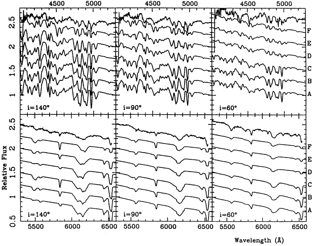
Fig. 19.— Two component models for Feige 7 using a surface ring of pure H on different helium‐rich background chemical compositions. The dipolar field strength is Bd = 35 MG with an offset az = 0.15. The observed spectra of Feige 7 are shown at the top of each panel in the blue (upper plots) and red (lower plots) spectral wavelengths, and the models are labelled by the viewing angle i. The letters on the right hand side of the figure denote the abundance geometry of the six synthetic spectra in each panel. Models A, B, and C have a hydrogen ring with a latitudinal extension of 60°, 40°, 20° (starting from θ lat = 100°), respectively, on a background of composition He∶H = 100∶1. Models D, E, and F have a have a hydrogen ring (with the same latitudinal extension as before) on a pure helium background. The data and models are from Achilleos et al. (1992a). Copyright Astrophysical Journal, reproduced with permission.
The presence of hydrogen‐ and helium‐rich regions is probably associated with the effects of a magnetic field on convective mixing. The magnetic field confines the motions of the stellar material along the direction of the field lines, thus inhibiting convection across field lines (Liebert et al. 1977; Achilleos et al. 1992a).
3.3.4. High‐Field Stars with Extreme Field Distributions
PG 1031+234 is a high‐field magnetic white dwarf with a rotation period of 3.4 hr. Schmidt et al. (1986a) and Latter, Schmidt, & Green (1987) estimated a field range of 500–1000 MG in this star, but the observed spectral variations cannot be modeled by a simple (dipole or offset dipole) global field distribution. They find that a localized region of high field strength (∼1000 MG) comes into view at certain rotational phases. They have proposed a two‐component model composed of a nearly centered dipole (Bd = 490 MG) and a strongly off‐centered dipole (az = 0.4) with a field approaching 1000 MG (a "magnetic spot"). The phase‐dependent data and the best‐fit model shown in Figure 20 are from Latter et al. (1987).
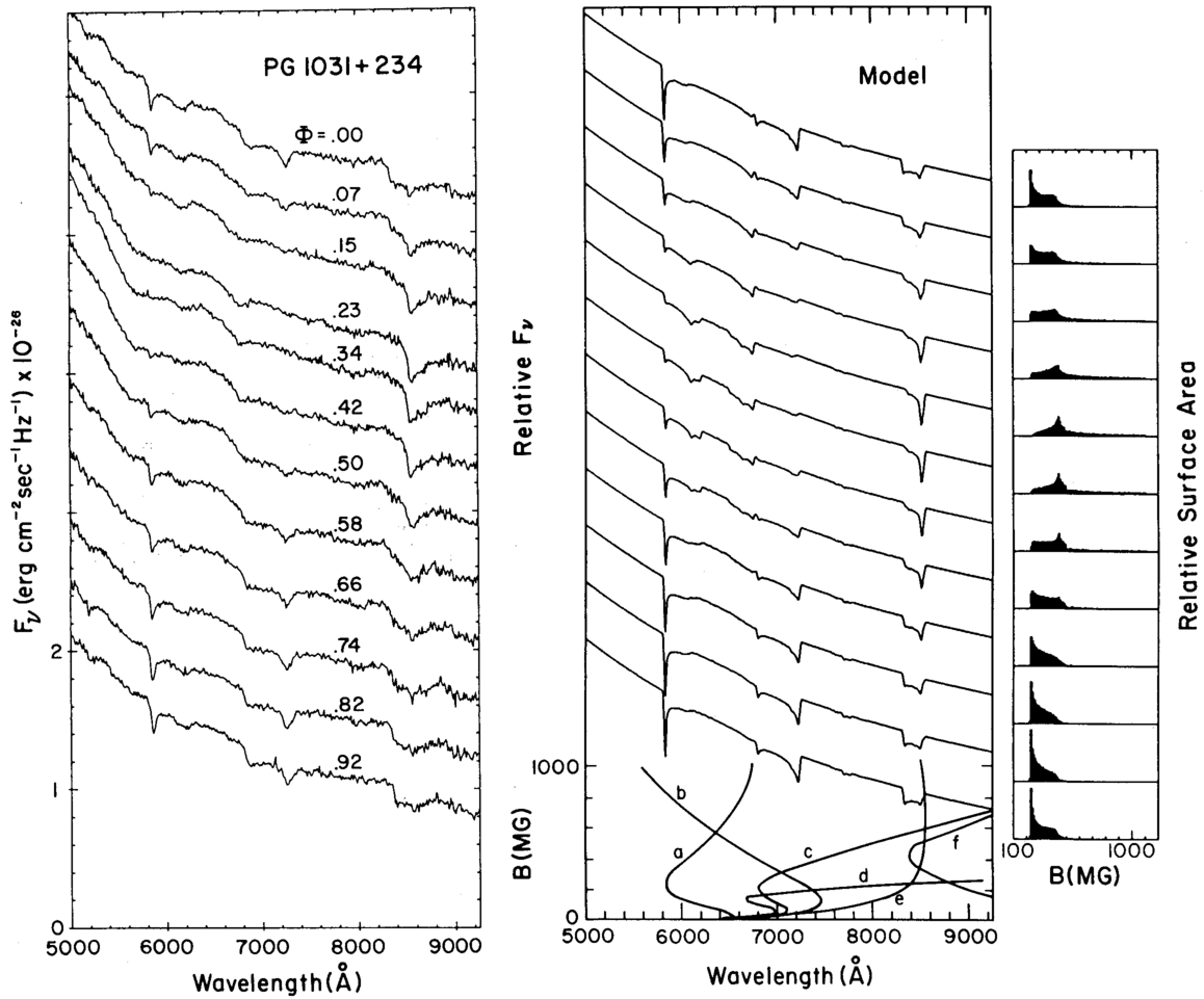
Fig. 20.— The observed phase‐dependent spectrum of PG 1031+234 (left panel) compared with a composite model consisting of a centered dipole and a strongly offset dipole (Schmidt et al. 1986a; Latter et al. 1987) (center panel). The curves at the bottom show the stationary Zeeman transitions of relevance to PG 1031+234 (Wunner et al. 1985). Displayed at right are histograms showing the observed stellar surface against the magnetic field strength. The data and model are from Latter et al. (1987). Copyright Astrophysical Journal, reproduced with permission.
A similar situation may occur with HE 1211−1707, which has been identified as a rotating magnetic white dwarf with spectral features varying on a period of about 110 minutes (Jordan 1997). The features are identified mostly with hydrogen (B∼80 MG), but the star shows large‐scale changes in its spectrum as a function of magnetic phase. There are no global simple field structures that have been found that can explain these variations.
3.3.5. WD 1953−01: A Low‐Field Star with a Spotlike Field Enhancement
The evidence for spotlike field enhancements also extends to very low field stars indicating that there may not be a correlation between field complexity and field strength.
WD 1953−011 shows spectral variations on a timescale of hours or days. The spectra at some phases can be modeled by a centered or nearly centered dipolar model with Bd = 100 KG. However, at other phases, a contribution is seen from a second region with a much stronger field of ∼500 KG. Detailed modeling by Maxted et al. (2000) has shown that the data require a localized high‐field region of field strength 490 ± 60 KG covering 10% of the surface area of the star superimposed on a weaker and more widespread field of mean strength 70 KG. Simple composite models consisting of centered and off‐centered dipoles of the type previously used to model isolated magnetic white dwarfs cannot explain the observed spectral variations. Data obtained 2 days apart are compared with the spot+dipole model in Figure 21.
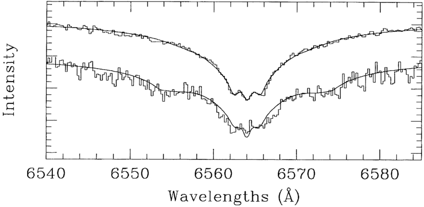
Fig. 21.— The observations of the low‐field MWD WD 1953−011 at two phases compared with a composite model consisting of a centered dipole with a field Bd = 100 KG and spot covering 10% of the area of the star with a field of 490 ± 60 KG. The spot is eclipsed at one phase and visible in the next.
3.4. Magnetic Double Degenerates
Studies of double degenerate stars (DDs) are important, particularly since one of the routes for producing Type Ia supernovae is the merger of such systems when the total mass exceeds the Chandrasekhar limit (Webbink 1979). Searches for close DDs have only yielded very few objects involving nonmagnetic WDs, and none of these has a total mass which exceeds the Chandrasekhar limit. According to population synthesis calculations of Yungelson et al. (1994), most candidate mergers are expected to be He+He or CO+He DDs, with a total mass less than the Chandrasekhar limit. On the other hand, CO+CO DDs may satisfy the required condition, though they appear to be much rarer. It has been suggested that the short‐period DD L870‐2 (Saffer, Liebert, & Olszewski 1988) may belong to the CO+CO or the CO+He class, but its total mass has been estimated to be ∼ 1 M⊙ (Bergeron et al. 1989). Of course, Type Ia supernovae may also occur at sub‐Chandrasekhar masses, for instance, as edge‐lit detonations of He on a CO WD.
The situation is somewhat different with the magnetic DDs. At present, there are only three known magnetic DDs, namely, EUVE J1439+75, LB 11146, and G64‐46. EUVE J1439+75 (Vennes et al. 1999a) is composed of a hot nonmagnetic DA white dwarf and a magnetic DA white dwarf. In this star, through detailed modeling, the spectra of the two components can be separated and analyzed. We show in Figure 22 the composite spectrum of EUVE J1439+75 compared with the model fits (Vennes et al. 1999a). The magnetic component is modeled with a centered dipole field of Bd = 14.8 MG. The total mass deduced from the two components is close to ∼ 2 M⊙,
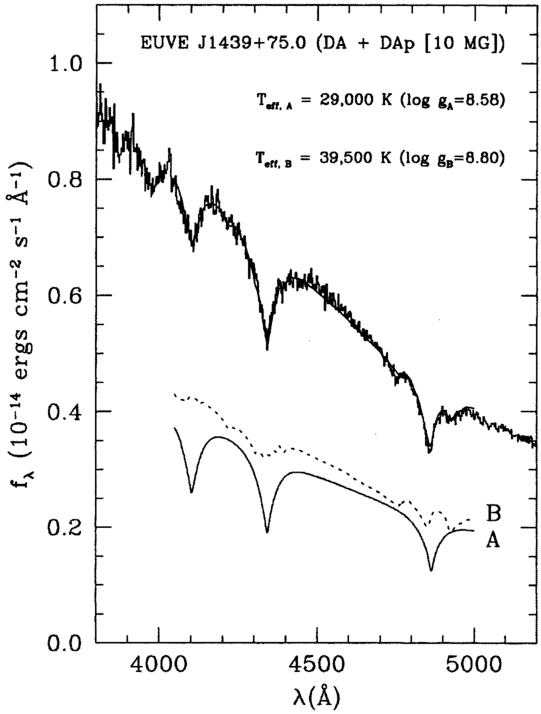
Fig. 22.— Top curves: Observed spectrum of the magnetic double degenerate EUVE J1439+75.0 with superimposed the best model fit (Vennes et al. 1999a). Bottom curves: Theoretical spectra of the two components: A (nonmagnetic DA) and B (magnetic DA). The resulting spectrum is well reproduced by a model with Teff = 29,000 K, log g = 8.58 for the A component and Teff = 39,500 K, log g = 8.8, and a dipolar magnetic field Bd = 14.8 MG viewed at i = 60° for the B component. Copyright Monthly Notices of the Royal Astronomical Society, reproduced with permission.
A closely related object, LB 11146, combines a normal DA white dwarf and a magnetic white dwarf of mixed composition (Liebert et al. 1993; Glenn, Liebert, & Schmidt 1994; Schmidt, Liebert, & Smith 1998) with a mean field of ∼670 MG. The mass and the temperature of the nonmagnetic component has been measured from line fitting and the temperature of the magnetic component from the broadband energy distribution. The assumption that they are at the same distance then yields a total mass of ∼ 1.8 M⊙. The third magnetic DD, G62‐46 (Bergeron, Ruiz, & Leggett 1993), is composed of a featureless DC white dwarf and a magnetic DA white dwarf. Bergeron et al. (1993) modeled the observed line profiles of the magnetic white dwarf with a dipolar field of Bd = 7.4 MG offset from the center of the star along the dipole axis by 0.07Rwd. There are no strong constraints on the total mass of this system. Thus, at least two of the three known magnetic DDs appear to satisfy the criterion for a Type Ia supernova of the standard type. The orbital parameters of the three DDs are not known. In LB 11146 strong upper limits have been placed on the velocity amplitude of the MWD which indicates that the system will not merge in a Hubble time (Glenn et al. 1994).
4. FUNDAMENTAL PROPERTIES OF ISOLATED MAGNETIC WHITE DWARFS
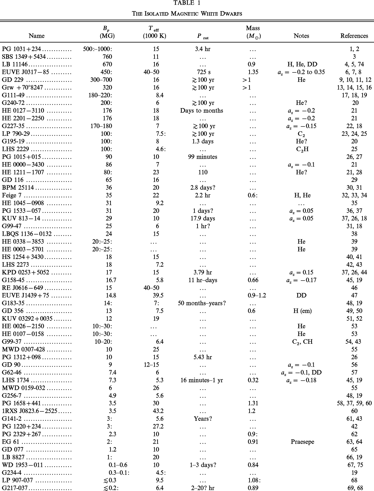
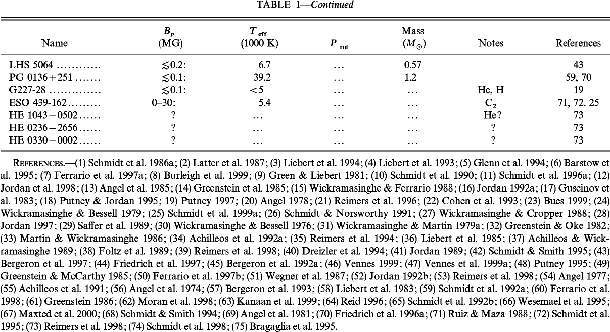
We present in Table 1 a comprehensive list of all known magnetic white dwarfs and their properties at the time of writing this review. The field strengths represent dipolar fields (that is polar fields) before offset, or average surface fields deduced from Zeeman spectroscopy or polarimetry. The upper limits given for the low‐field objects are estimates based on measured longitudinal fields from Zeeman spectropolarimetry. There are 65 objects in the list, and there are estimates or upper limits for the magnetic field in all but three objects, and estimates of the masses for 16 stars. The objects at the bottom of the list are also very likely to be high field, but no Zeeman estimates are available.
4.1. Field Distribution
Magnetic white dwarfs are detected either as peculiar objects in spectroscopic surveys or in polarization surveys of white dwarfs. The early surveys exhibited a strong bias toward the cooler stars, but in more recent years hotter objects have been discovered from the Palomar‐Green, ESO‐Hamburg, EUVE, and ROSAT surveys. The spectral resolution of most spectroscopic surveys enable only the higher field objects (B≳106 G) to be recognized through the Zeeman splitting of the lines.
In an attempt to push the field limits to lower values, Schmidt & Smith (1995) carried out a comprehensive survey of the brightest 170 DA white dwarfs accessible in the northern hemisphere using high signal‐to‐noise ratio circular spectropolarimetry of the Hα line. They discovered several low‐field stars and allowed limits to be placed on other stars with a mean uncertainty for longitudinal fields of 8600 G. The lowest field measured in this survey was that of G217‐037 with a mean longitudinal field varying in the range -100 ± 15≲Bl≲ + 9 ± 12 KG. The magnetic field distribution, when considered as a percentage discovery basis, showed the incidence of magnetism to be consistent with approximately 1% per decade above 30 KG in the field range 30 KG–1000 MG, but the statistical errors were large below 0.1 MG.
More recently, circular spectropolarimetric observations across Hα at a resolution of 0.5 Å and hydrogen line magnetometer observations of the wings of Hβ and Hγ have been used to place upper limits of 500 G–50 KG on the field strengths of 17 white dwarfs (Fabrika & Valyavin 1999a). Schmidt & Grauer (1997), using circular spectropolarimetry, placed a stringent upper limit of ≲1 KG on the longitudinal magnetic field of four pulsating white dwarfs. There is some indication, therefore, that the magnetic field distribution may in fact turn over at ≲0.1 MG, although given the different levels of sampling across different field ranges, it may be premature to reach such a conclusion at the present time.
Most stars have directly measured field strengths from the Zeeman effect in H, He, or CH. These span the field range 3 × 10⁵–109 G. A few are classified as strongly (≳100 MG) magnetic purely on the basis of a peculiar absorption‐line spectra. This is defendable for the hotter stars since the Zeeman effect of H, He i (most optical lines), and He ii is well established for fields below this range. A few others are known to be strongly magnetic through broadband polarization measurements (e.g., G270‐42), but accurate field estimates are not possible because the spectroscopic features have not as yet been identified.
The normalized histogram for the field distribution of the magnetic white dwarfs in Table 1 is shown in Figure 23. The sample yields 〈log B(MG)〉 = 1.193 ± 0.741 (〈B〉 = 15.6 MG). It is evident from this figure that the earlier result by Angel, Borra, & Landstreet (1981) based on a significantly smaller sample of stars, namely, of an equal number of MWDs per decade in field, is still correct to within a factor of 2, but only for fields in excess of 10 MG.
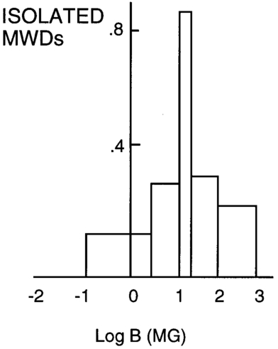
Fig. 23.— Normalized histogram of the field distribution of all magnetic white dwarfs in Table 1.
The number of magnetic white dwarfs in Table 1 compared with the total number of white dwarfs in the McCook & Sion (1999) catalog (∼1280) suggests that 5.1% are magnetic. This is marginally higher than the estimate given by the magnitude limited sample of Schmidt & Smith (1995), who found that 4.3% were magnetic. Using the space density 0.003 pc−3 of white dwarfs estimated by Liebert, Dahn, & Monet (1988), the space density of MWDs with fields in the range 30 KG–1000 MG is 1.5 × 10⁻⁴ pc−3.
There was an early suggestion based on the very small sample of nearby WDs that the incidence of magnetism was higher among the cooler stars (Liebert & Sion 1979), with obvious implications for theories on the evolution of the magnetic field along the cooling sequence. The number of hot WDs that have been recognized as magnetic has increased significantly in recent years. Table 1 shows that there now are an approximately equal number of MWDs between 5000 and 10,000 K as there are between 10,000 and 20,000 K, with the number dropping off rapidly at higher temperatures. However, given the different biases toward higher or lower temperature stars in the various surveys contributing to Table 1, these results cannot easily be used to revisit the problem of the incidence of magnetism. Fabrika & Valyavin (1999b) have, however, recently argued that the trend noted by Liebert & Sion (1979) persists in the enlarged sample of MWDs.
4.2. Atmospheric Composition
The majority of the stars in Table 1 show Zeeman‐split hydrogen lines and have hydrogen‐rich atmospheric compositions similar to the (nonmagnetic) DA white dwarfs. The star Feige 7 shows a mixed composition as is evidenced by the presence of both hydrogen and neutral helium lines in its spectrum. The high‐field (7 × 10⁸ G) star LB 11146 (Liebert et al. 1993; Glenn et al. 1994) may be another member belonging to this mixed composition class. These stars are expected to have helium‐rich compositions with traces of carbon and/or hydrogen in their atmospheres. More recently, the ESO‐Hamburg survey has resulted in the discovery of four new low‐field magnetic DB white dwarfs, HE 0338−3853, HE 0003−5701, HE 0338−3864, and HE 0107−0158 (Reimers et al. 1998). Similarly, the stars HE 0236−2656, HE 1043−0502, and HE 0330−0002 show structure with some similarities to GD 229, suggesting that they may also be magnetic with helium‐rich atmospheres (Reimers et al. 1998).
From Table 1, 20% of the magnetic white dwarfs are found to have helium‐rich atmospheres similar to the situation with the nonmagnetic stars. Helium‐rich stars which show traces of H in their atmospheres appear however to be more common among the magnetic stars (e.g., Feige 7, LB 11146). If convective mixing is responsible for the DB phenomenon, as is currently believed to be the case, this observation suggests that mixing may be inhibited at strong fields (Achilleos et al. 1992a).
4.3. Rotational Periods
If angular momentum is conserved in the post–main‐sequence phase of evolution, the rotational velocities of the white dwarfs should be near the breakup value. However, the nonmagnetic white dwarfs, as a class, tend to be slow rotators. A stringent upper limit of vsin i≲30 km s−1 has bee placed on 13 DA WDs by Heber, Napiwotzki, & Reid (1997), with a limit as low as vsin i≲8 km s−1 for 40 Eri B using Keck observations. The implied rotational periods are Prot≳1 hr. Firm determinations of the rotational velocities have been possible for the three WDs PG 1159−035, PG 0122+200, GD 358 (Winget et al. 1991, 1994; O'Brien et al. 1996) and the central star WC3 of the planetary nebula NGC 1501 (Bond et al. 1996) using quite a different technique, namely, the rotational splitting of oscillation modes in asteroseismology. The rotation periods of these stars range from 1.17 to 1.6 days, indicating that periods of ∼day may be typical for isolated nonmagnetic WDs. All these results suggest efficient angular momentum transfer from the core to the envelope and large‐scale angular momentum loss during post–main‐sequence evolution. Although the details of this process are unclear, one may expect that the MWDs should be even slower rotators because the magnetic fields are likely to lead to increased braking of the stellar core as it approaches the WD state. This is particularly so, since their likely progenitors, the magnetic Ap and Bp stars, are known as a class to be slow rotators (Borra, Landstreet, & Mestel 1982).
The observations of isolated MWDs tend in general to support this expectation. Strong limits can be placed on rotation by looking for variations in polarization or polarization angle. The largest measured rotation period is 17.9 days for KUV 18134−14 (see Table 1). However, searches for changes in the polarization angle in several high‐field MWDs such a Grw +70°8247, G227‐35, LP 790‐29, and G240‐72 over periods of tens of years have led to negative results. These star must have a rotation period of ≳100 yr (West 1989; Schmidt & Norsworthy 1991). Extreme slow rotation may therefore be a characteristic of the large majority of the MWDs.
However, there is also a class of rapidly rotating MWDs typified by Feige 7 (3 hr), PG 1031+254 (3 hr), and the recently discovered high‐field star EUVE J0317−855 (725 s) (see Table 1). For these stars, the rotation periods appear to be significantly higher than for nonmagnetic white dwarfs. What is surprising is that the strong magnetic fields have not been effective in spinning down these stars, whereas they appeared to have played just such a role in most MWDs.
The case of EUVE J0317−855 may be special since this star is likely to be the result of a DD merger. However, the spin up of a compact star, if it is magnetic, during the mass transfer phases of close binary evolution, is an expected phenomenon and has, for instance, been used to explain the millisecond pulsars. The spin of the other rapidly rotating magnetic white dwarfs may be the result of accretion torques during binary star evolution regardless of whether a merger has occurred. Indeed, in the phase‐locked AM Her systems, the MWDs are known to have periods of ∼hours. It has been proposed that stars such as PG 1031+254 may be the end product of the orbital evolution of the AM Herculis–type binary systems, in which case these stars may have planetary‐mass companions.
MWDs may therefore consist of two populations depending on whether they result from single star evolution or binary star evolution. EUVE J0317−855 may be an extreme case where close binary evolution resulted in a merger (Ferrario et al. 1997a). This apparently bimodal distribution is shown in Figure 24 constructed from all stars in Table 1 with measured or estimated rotation periods. The stars with estimated rotation periods of greater than 100 yr have been artificially placed in the last bin, so that the second peak could be much broader extending to longer periods.
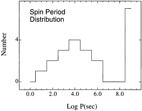
Fig. 24.— Distribution of rotation periods of magnetic white dwarfs in Table 1. The stars with rotation periods of greater than 100 yr are placed in the last bin.
4.4. Mass Determinations
Greenstein & Oke (1982) used the trigonometric parallax and an estimate of its effective temperature to deduce that Grw +70°8247 has a mass greater than 1 M⊙. Liebert (1988) showed that several other MWDs with measured parallaxes lie below the Mv‐Teff diagram for normal WDs and proposed that the MWDs may as a group have a higher mean mass. This conjecture gained support from studies of the tangential space motions of white dwarfs which suggested that the MWDs have lower than average tangential space motions (Sion et al. 1988) and may therefore have been drawn from a younger parent population. The mass estimates for the higher field stars (Table 1) are based on trigonometric parallaxes or binary star membership. For the low‐field stars, the masses are from model atmosphere analyses assuming standard (zero magnetic field) Stark broadening theory (see § 2.3). The results are illustrated in the mass distribution of the MWDs in Table 1 shown in Figure 25. When only a lower limit is available for a particular star, we have used this limit for the mass.
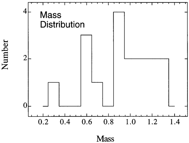
Fig. 25.— Mass distribution of magnetic white dwarfs in Table 1
In recent years it has become apparent that the mass distribution of the nonmagnetic white dwarfs is bimodal, with the main peak occurring at 0.57 ± 0.02 M⊙ and a much smaller secondary peak at 1.2 M⊙ (Vennes 1999). The origin of the second peak remains a mystery, with one explanation being that these stars may be the result of binary star mergers of the CO‐CO type. The argument against this hypothesis has been that there do not appear to be any obvious DD candidates of the nonmagnetic variety with a total mass of 1.2 M⊙ which will explain this peak. Most appear to be CO‐He DDs with a total mass of 0.9 M⊙ (Maxted & Marsh 1999), consistent with expectations from binary star evolution (Yungelson et al. 1994).
When one looks at the MWDs a different picture emerges. Of the three magnetic DDs that have been discovered, two appear to have a total mass above the Chandrasekhar limit (§ 3.4). There is also the interesting observation (Vennes 1999) that of the 15 ultramassive white dwarfs (M>1 M⊙) discovered from the EUVE survey, an anomalously large fraction (25%) are magnetic. Of this sample, the WDs that have masses that are closest to the Chandrasekhar limit (≳ 1.3 M⊙) and may be the result of a merger are both magnetic! These results suggest that the magnetic DDs are more likely than nonmagnetic DDs to be progenitors of type Ia supernovae which result from tipping of a CO WD above the Chandrasekhar limit.
In the MWDs we may be seeing a magnetic manifestation of the evolution scenarios (single star or interacting binary) responsible for the bimodal mass distribution of nonmagnetic white dwarfs. An interesting possibility is that the MWDs cluster around a mass peak corresponding to single star evolution from progenitor magnetic Ap and Bp stars (see § 5) with possibly a second peak arising from binary star evolution, with both peaks shifted toward higher masses. The shift toward higher masses may simply indicate that magnetic fields play an important role in post–main‐sequence evolution controlling both mass and angular momentum loss, resulting in a different initial‐final mass relation for the magnetic stars. An intriguing possibility is that close binary evolution involving magnetic stars may lead to a different frequency of DDs and of systems which may lead to mergers. This hypothesis needs to be tested against a larger sample of magnetic white dwarfs, but if confirmed it will have important implications for the birth rate of Type Ia supernovae. Given the difficulties in modeling the atmospheres of magnetic white dwarfs of arbitrary field strength, a definitive investigation of this type is clearly not possible at the present time (see, however, Valyavin & Fabrika 1999).
4.5. The Origin of the Magnetic Fields
In the early‐type main‐sequence stars, magnetic fields (∼102–104 G) are found only in the Ap and Bp stars. Stringent upper limits of ≲1 G can be placed on other "nonmagnetic" A and B stars. The fields in the Ap and Bp stars are likely to be fossil relics of star formation, while in stars of spectral type later than F0, where the stellar envelopes are convective, the fields are most likely to be dynamo generated. Centered or mildly offset dipoles, and in some cases quadrupoles, appear to represent the observations of these stars reasonably well (Borra et al. 1982). The field decay times are generally larger than the stellar evolution time, and it is likely that these fields are fossil (Mestel 1999).
When one turns to the magnetic white dwarfs, the observed field distribution appears to be pointing to a similar situation, except that the field spread is about a factor 100 larger, ranging from ∼105 to 109 G, peaking at 1.6 × 10⁶ G. Attempts at measuring lower fields have led to negative results in most cases, indicating perhaps that the field distribution turns over at about 105 G.
It is therefore tempting to identify the progenitors of the magnetic white dwarfs resulting from single star evolution to be the Ap and Bp stars. Magnetic flux conservation of a fossil field could then lead naturally to the observed field distribution in white dwarfs as the star contracts in radius by a factor of 100 as it evolves toward the white dwarf sequence. The estimated birth rate of magnetic white dwarfs appears to be generally consistent with this hypothesis (Angel, Remillard, & Wickramasinghe 1981). The long ohmic decay times estimated for the lower order field components (Wendell, Van Horn, & Sargent 1987; Muslimov, Van Horn, & Wood 1995) in white dwarfs are also consistent with a fossil origin for the fields.
An interesting method of testing the fossil theory has recently been proposed by Kanaan, Claver, & Liebert (1999). On the assumption of coeval star formation in clusters, clusters young enough for Ap stars not to have evolved off the main sequence should not show evidence of magnetism in the white dwarfs. On the other hand, clusters old enough for Ap stars to have evolved off the main sequence should show some MWDs. The first results reported for Praesepe showed a massive (0.912 M⊙) magnetic white dwarf EG 61 with a field of 2 MG and other normal‐mass (∼0.6 M⊙) nonmagnetic WDs and one low‐mass nonmagnetic WD. From the age of the cluster (1 Gyr), and the estimated cooling age of the MWD, the progenitor mass of the MWD is estimated to be 2.2 M⊙, which is in the mass range where Ap stars are found. Thus, in Praesepe, the most massive WD is magnetic, which adds support to the view discussed in the previous section; namely, the magnetic field inhibits mass loss in post–main‐sequence evolution and favors the formation of more massive WDs.
4.5.1. Field Structure
Schmidt & Norsworthy (1991) have observed nearly pure sinusoidal variations in the broadband circular polarization of four rotating MWDs and strongly nonsinusoidal variations in one star, namely, PG 1031+234 (Schmidt et al. 1986a). However, higher order components would tend to cancel in circular polarization when averaged over the stellar disk, and these results cannot, on their own, be used to infer the presence of pure dipolar fields in these four stars. As already noted, there is strong evidence from Zeeman spectroscopy for complex nondipolar fields in several MWDs.
The question of field strength and complexity of the currently observed sample is expected to be related to the origin of the magnetic field and its evolution as the WD cools. We have searched for correlations between magnetic field and mass and found none, but the masses are only known for a very few objects. There does not appear to be any correlation between magnetic field strength and effective temperature (or, equivalently, cooling age), but the expected field decay of the dipolar component in the simplest models is small (see below). The relevant plots are shown in Figure 26.
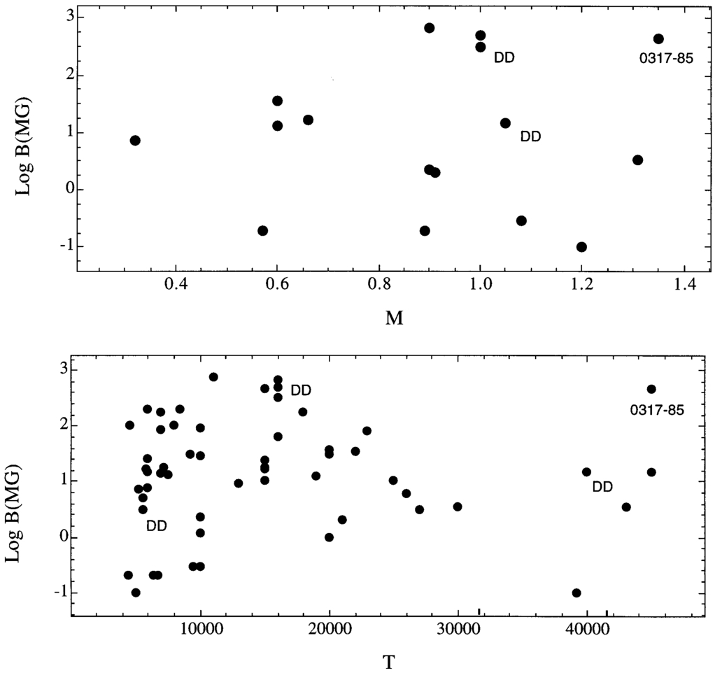
It is more difficult to investigate whether there is any evidence for the evolution of the complexity of the field with age. The well‐studied rotating MWDs all have temperatures above 10,000 K, and these show evidence of off‐centered (or more complex) field structures. However, examples of cool rotating MWDs which have been studied in the same detail using Zeeman spectroscopy are less common. Of the two stars which have shown evidence for spot‐type field structures, one (PG 1031+254) has a high field and the other (WD 1953−011) a low field.
The early work of Chanmugam & Gabriel (1972) and Fontaine, Thomas, & Van Horn (1973) showed that the timescale for the free ohmic decay of the low‐order poloidal and toroidal components would typically exceed the cooling time of a white dwarf (∼1010 yr) supporting a fossil origin for the fields. Wendell et al. (1987), and subsequently Muslimov et al. (1995), incorporated more realistic stellar models along the cooling sequence and improved expressions for the conductivity. The latter authors found that the surface dipolar component decays by a factor of 2 in 109 yr for a 0.6 M⊙ white dwarf when the matter in the deep interior is in the Coulomb liquid regime. Thereafter the decay occurs on a timescale of 1010 yr. These calculations also showed that the higher order components decayed significantly faster, so that the presence of dominant quadrupolar or higher order components in MWDs were difficult to explain on these free ohmic decay models. Even though the Ap and Bp stars do show evidence for complex field structures, the complex field structures seen in the MWDs were therefore unlikely to be fossil remnants of this phase.
Driven by the growing evidence for complex field structures in white dwarfs, Muslimov et al. (1995) included an additional ingredient in the field decay models—namely, the Hall drift. The Hall drift effectively couples the different poloidal modes in a nonlinear manner, so that the field decay is no longer "free ohmic." They present a scenario in which the white dwarf acquires a strong (109 G) toroidal field through differential rotation in the pre–white dwarf phases of evolution in addition to a poloidal component. The inclusion of the Hall effect allows the field to continue to evolve after the core has frozen. Through the nonlinear coupling, the higher order poloidal components may in fact be amplified relative to the dipolar component, and under certain circumstances a relative amplification by up to a factor of ∼2–20 of the quadrupolar component was found to occur on a timescale of 1010 yr. The calculations also showed that the field decay of the dipolar component and the relative amplification of the quadrupolar mode were strong functions of the mass of the WD. The Hall effect may therefore play a critical role in explaining the bizarre field structures seen in magnetic white dwarfs. The magnetic spot–type structure deduced in some stars may require, in addition, the relaxation of the force‐free assumption which has so far been made in all field decay calculations.
5. THEORETICAL CONSIDERATIONS
5.1. The Polarized Transfer Equations
As we have already seen, the magnetic field introduces a directional and polarizational asymmetry in the absorption processes, and these and related effects have to be taken into consideration in formulating the transfer equations. The transfer equations can be derived classically from the dielectric tensor formalism for describing the propagation of polarized EM radiation through a magnetized medium (e.g., Pacholcyzk 1976) or can be derived in the quantum limit using the density matrix description of polarized light (Landi Degl'Innocenti & Landi Degl'Innocenti 1972). In general, the solution of the dispersion relationship yields two modes (the normal modes) with refractive indices n1 + iκ1 and n2 + iκ2, respectively, that will propagate with the polarization state unchanged through the medium. The imaginary parts yield the absorption terms, and the differences in the absorption between the two modes give rise to magnetic dichroism. The real parts specify the phase velocities, and the differences in the phase velocities between the two modes and give rise to magnetic birefringence. A wave of given polarization will in general change its polarization state as it propagates through the atmosphere due to both effects.
5.1.1. The Pure Absorption Case
Unno (1956) was the first to formulate the radiative transfer equations for a normal Zeeman triplet in pure absorption in a stellar atmosphere (the Sun). He envisaged the atmosphere as being composed of an ensemble of linear and circular oscillators of the π and σ types following the classical theory of Lorentz. His formulation allowed for magnetic dichroism in the atmosphere, but neglected magnetic birefringence, but these were included subsequently. The polarized radiative transfer equations for a plane‐parallel atmosphere in the absence of scattering and assuming LTE can be written quite generally as (Hardorp, Shore, & Wittman 1976; Martin & Wickramasinghe 1979b)

where

Here I is the Stokes vector and B is the Planck function; μ is the cosine of the angle made by the direction of propagation and the outward normal to the atmosphere, τ is the optical depth perpendicular to the atmosphere corresponding to a standard opacity κstd. The η and ρ terms are the absorption and rotation matrices normalized to the standard opacity and result from magnetic dichroism and magnetic birefringence, respectively:
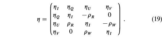
Landi Degl'Innocenti & Landi Degl'Innocenti (1981) have argued from quite general principles that the transfer equation for polarized radiation must have the above form and symmetry properties, regardless of the details of the absorptive and emission processes.
The terms ηI,ηQ,ηU, and ηV in the absorption matrix allow for selective absorption in the Stokes intensities I,Q,U, and V, respectively, and arise from the imaginary parts of the refractive indices which describe the polarization eigenmodes which propagate through the medium. The terms ρR and ρW arise from the real parts of the refractive indices and allow for difference in phase velocity and phase mixing of the polarization eigenmodes. These are the terms which include effects such as Faraday rotation and the Voigt effect (Martin & Wickramasinghe 1981). The particular form of η in the above equation (without a term in ηU) arises from the choice of coordinate system where the x‐direction (used to measure wave polarization) has been chosen to be in the plane containing the field direction and the direction of wave propagation.
The action of the antisymmetric part of the matrix η, which carries the Faraday terms, is to simply convert one type of polarization into another. These terms do not change the degree of polarization. The symmetric part of the matrix η, on the other hand, selectively absorbs particular types of polarization and reemits as unpolarized radiation. They result in both an attenuation of the radiation and a change in the degree of polarization.
In most cases, we deal with dipole radiation, and in this case ηI,ηQ,ηU, and ηV can be written as
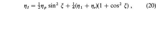


where ξ is the angle between the direction of wave propagation and the field direction; ηp is the normalized (relative to the standard opacity) absorption coefficient for linearly polarized radiation propagating perpendicular to the field with the electric vector in the field direction. They arise from π transitions (p components) for which the change in the magnetic quantum number Δm = 0. Terms ηl and ηr are the (normalized) absorption coefficients for left‐ and right‐circularly polarized radiation propagating along the field and arise from σ+ (Δm = -1, the l components) and σ- (Δm = +1, the r components), respectively. Likewise the rotation terms can be expressed as


where fp,fl, and fr arise from differences in phase velocities of orthogonal polarization states for waves propagating perpendicular to the field (the two linear modes with polarization along and parallel to the field) and along the field direction (the left‐ and right‐circularly polarized modes).
The solutions of these equations are usually carried out using a piecewise solution following Martin & Wickramasinghe (1986) or a fourth‐order Runge‐Kutta method.
5.1.2. The Inclusion of Electron Scattering
So far, only pure absorption models have been used to analyze individual stars. If scattering is important in the continuum, the transfer equation takes the form
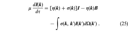
The additional terms include an extinction matrix σ and a scattering phase matrix σ(k,k') which reduces to the Rayleigh matrix in the limit of zero field. We refer the reader to Dittman & Wickramasinghe (1999) for expressions for the field‐dependent source function for Thomson scattering. These equations have so far been solved in the pure scattering limit using Monte Carlo techniques for plane‐parallel geometries and a dipole field distribution (Whitney 1991a, 1991b) and in the more general case allowing for scattering and absorption using numerical integration of the equations by Dittman & Wickramasinghe (1999). There have been no applications of these models to hot magnetic white dwarfs as yet.
5.2. Line Opacities
The Zeeman theory gives the wavelengths and the transition probabilities, but the calculation of the absorption cross sections require a knowledge of line broadening.
For a Voigt profile which includes thermal Doppler broadening and pressure broadening as a damping parameter in a Lorentzian profile, the absorption and rotation terms are given by
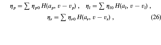
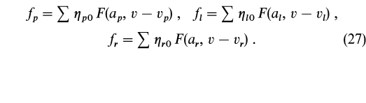
The summations are over the individual p, l, and r components in the blend; H(a,v) is the Voigt function and F(a,v) the associated dispersion function given by
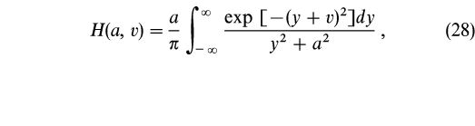
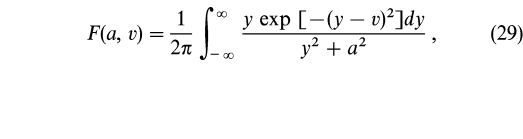
where a = γλ2/4πcΔλD is the damping parameter and v = Δλ/ΔλD. Terms vp, vl, and vr are the Zeeman shifts of the p, l, and r components in units of ΔλD, and ηp0, ηl0, and ηr0 are the values of η at the line centers at zero damping. These quantities are calculated using the tabulated values of the positions and strengths of the Zeeman components as a function of field strength given by atomic physics calculations (§ 2.1). As was shown by Martin & Wickramasinghe (1981) and subsequently by Jordan, O'Connell, & Koester (1991), the rotation terms (giving rise to "magneto‐optical effects") play an important role in determining the relative strengths of σ and the π components, and the line profiles and polarization.
5.3. Continuum Opacities
The construction of model atmospheres and theoretical spectra requires a detailed knowledge of the effects of the magnetic field not only on line shifts and oscillator strengths but also on continuum opacities and on pressure (in particular, Stark) broadening which determines line opacities.
One of the major obstacles has been the intrinsic difficulty in carrying out atomic physics calculations of energy levels and cross sections in strong magnetic fields in the regime of mixed (spherical and cylindrical) symmetries where both Coulomb and magnetic effects are of comparable importance. As already noted, this problem has essentially now been solved for bound‐bound levels of H and He. To calculate bound‐free and free‐free transitions, one needs also to consider the continuum as being quantized into quasi (because of the electrostatic interaction) Landau levels.
5.3.1. Bound‐Free Opacity of Hydrogen
The bound‐free opacity of hydrogen in the presence of a magnetic field was first considered by Lamb & Sutherland (1974). They argued that since in the linear Zeeman regime the frequencies are shifted by the Larmor frequency ωL = 1 / 2 ωC independently of the principal quantum number n, a bound‐free edge will split into three edges separated by ωL in much the same way as a line splits into a Lorentz triplet. Assuming further that the wave functions of bound electrons and free electrons close to the atom are unperturbed (rigid) to first order in the magnetic field, they argued that bound‐free opacities in a magnetic field can be calculated from the zero‐field opacities κ = ωg(ω) from
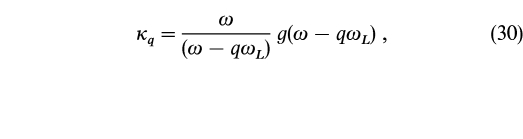
where q = 0, + 1, and −1 for κp,κr, and κl, respectively. Thus, the continuum opacity in a magnetic field was obtained from the opacity in the absence of a magnetic field by simply "shifting" the opacity according to the above equation. This assumption formed the basis for calculations of bound‐free opacities for H, He i, He ii, and H− in all model atmosphere calculations in the low‐field linear Zeeman regime prior to 1988.
Jordan (1989) pointed out that this procedure was invalid even in the linear Zeeman regime since the energy levels of free electrons are separated not by the Larmor frequency ωL but by the cyclotron frequency ωC. In fact the free electron has discrete energy levels for motion perpendicular to the field (the Landau states) with energies given by
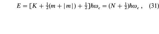
where K(≥0) is an integer and N(≥0) and m are the quantum numbers for energy and the z component of angular momentum, respectively. Thus N = 0 (the lowest energy state) corresponds to (K,m) = (0, 0),(0, -1),(0, -2),(0, -3),...; N = 1 to (K,m) = (0, 1),(1, 0),(1, -1),(1, -2),...; etc.
Since the motion in the z‐direction is free, a Landau continuum will be built upon each of the (N,m) Landau thresholds, and these will give rise to bound‐free absorption. Jordan (1989) argued that of all the allowed transitions (Δm = 0, -1, and +1) from bound states to Landau states, the dominant contribution to the opacity will come from transitions to the Landau states of the lowest possible energy. Using the energy levels for bound states calculated by the Tübingen group, it was then possible to calculate accurate wavelengths for the bound‐free edges. The Balmer edge was now split into 12 components and the Paschen edge into 26. The absorption cross sections were again calculated assuming the rigidity approximation for the wave functions as in Lamb & Sutherland (1974), with the zero‐field opacity distributed among the various components not equally but using the Wigner‐Eckart theorem.
The first extensive calculations of the bound‐free absorption cross sections for hydrogen were recently published by Merani, Main, & Wunner (1995). These detailed numerical calculations represent a major advance in the area of strong‐field (β≥1) atomic physics and show that the situation is more complicated than envisaged by Jordan (1992a). The appropriate energy level diagram is given in Figure 27, where the lowest lying bound and free states have been grouped according to m manifolds and the allowed transitions shown. The Merani et al. (1995) calculations show the presence of strong resonances superimposed upon each of the Landau continua, and these resonances tend to dominate the bound‐free cross sections. Furthermore, significant opacity could result from transitions to higher Landau states. A particularly interesting result is that in the strong‐field regime, the dominant opacities occur for σ+ transitions—as already noted, this is the natural sense of absorption for electrons in a magnetic field.
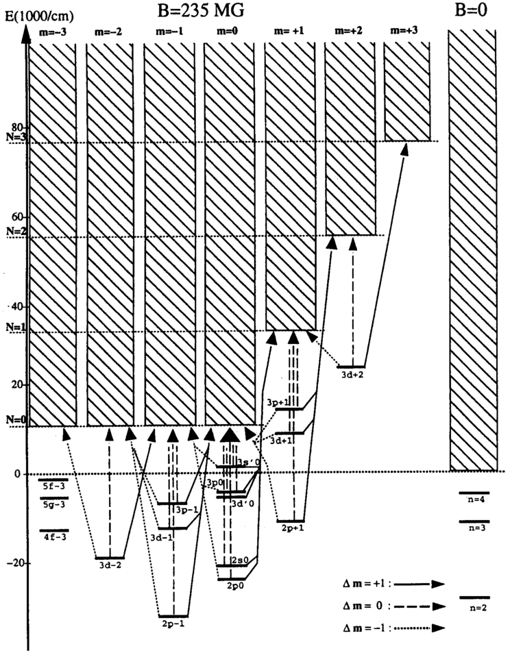
Fig. 27.— The energy level diagram for low‐lying bound states and continuum states of hydrogen ordered according to their m quantum number for B = 235 MG. The allowed bound‐free transitions and the associated Landau continua are also shown (from Merani et al. 1995). Copyright Astronomy and Astrophysics, reproduced with permission.
The results of calculations of the Balmer and Paschen bound‐free opacity for a plasma with a temperature of 50,000 K in the narrow field range 1.17 × 10⁸– 2.35 × 10⁸ G are shown in Figure 28. Unless the field is nearly uniform over the visible disk, we do not expect any of the narrower resonance type features shown in Figure 28 to be detected as individual lines in the spectrum; they will simply be broadened out into a smooth continuum by field spread.
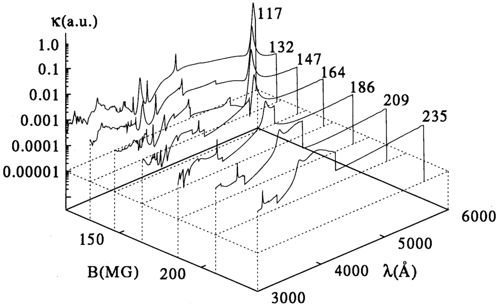
Fig. 28.— The bound‐free Balmer and Paschen opacities for the Δm = 1 transitions of hydrogen for the field range 1.17 × 10⁸ G − 2.35 × 10⁸ G at a temperature of 50,000 K from Merani et al. (1995). Copyright Astronomy and Astrophysics, reproduced with permission.
The new opacities are presently unavailable in a form that can readily be incorporated in model calculations. Attempts at including these opacities in model atmosphere calculations (Jordan & Merani 1995) have shown no significant improvements in model fits to continuum observations of high‐field stars in comparison to what can be achieved from the simpler approach adopted by Jordan (1989).
5.3.2. Free‐Free or Magneto‐Bremsstrahlung Opacity
The radiation emitted by a free electron as it accelerates past an ion in the presence of a magnetic field is known as magneto‐bremsstrahlung. Classical expressions for this opacity are readily available (e.g., Pacholcyzk 1976), and these have so far been used in all model atmosphere calculations for MWDs in the low‐field approximation, where the collisional frequency is assumed to be independent of the field. However, in the context of high‐field magnetic white dwarf atmospheres, additional structure may appear at the cyclotron resonance frequency and its harmonics simply due to the directional dependence of the collisional frequency in the presence of a magnetic field (Pavlov & Shibanov 1978).
5.3.3. Hydrostatic Equilibrium
The magnetic field can affect atmospheric structure directly through its influence on the hydrostatic equilibrium. Landstreet (1987) considered this possibility in the context of Ap stars and white dwarf atmospheres and showed that the ohmic decay of a global magnetic field will induce atmospheric currents which could, under certain circumstances, result in a sizeable Lorentz force. The details depend on the rate of decay of the field, atmospheric composition, and temperature. For an H atmosphere, and for the decay of the dipolar component in a low‐mass MWD (M≲0.6 M⊙), the atmospheric structure could be affected up to optical depth 10 provided T≳12,000 K. The decay‐induced Lorentz force has so far not been included in model atmosphere calculations.
5.4. Normal Modes of Propagation
Useful insights into the properties of magnetic atmospheres have been obtained by formulating the transfer equations in terms of the normal modes of propagation. In an anisotropic medium, it is generally possible to identify two eigenmodes (the "normal" modes), each with a characteristic polarization that will propagate through the plasma independently of each other provided scattering and radiation processes are unimportant. The intensities I1 and I2 of these two normal modes (also referred to as the extraordinary and the ordinary modes), and two other intensities I+ and I- which specify the phase relationships between them, describe the radiation field completely and can be used in place of the Stokes intensities (I,Q,U,V).
The transfer equations when formulated in terms of (I1,I2,I+,I-) have the following properties. First, if the phase shift between the two normal modes owing to propagation through unit optical depth is large, the solution to the transfer problem in an optically thick medium is given entirely in terms of the intensities I1 and I2 of the two normal modes, independently of I+ and I-. This is referred to as the limit of large Faraday rotation. The condition for this limit is ω(n1 - n2)/c≫(κ1 + κ2)/2, where n1 and n2 are the refractive indices and κ1 and κ2 are the absorption coefficients of the two normal modes (Gnedin & Pavlov 1974).
There is another situation related specifically to semi‐infinite atmospheres when the normal‐mode formulation could also be useful. This occurs if the normal modes have orthogonal polarizations (that is, the polarization ellipses are similar and their principal axes orthogonal). Then, the equations for I+ and I- do not have a source term and hence die off to zero at the surface. In both these cases, it is clearly more advantageous to work with the intensities of the normal modes, rather than the Stokes intensities linked to the Cartesian basis, since only two uncoupled differential equations then need to be considered. The normal‐mode formulation also allows an easy generalization to include scattering (Kaminker, Pavlov, & Shibanov 1982), which then couples the equations.
The transfer equations for the pure absorption LTE case when the modes of propagation are orthogonal are (Lamb & Sutherland 1974)
where ηk(n) = κk(n)/κstd is the ratio of the true absorption coefficient for the kth mode propagating along the direction n to the standard absorption coefficient κstd which defines the standard optical depth scale τ.
In the simple case of a source function B(τ) = B0(1 + βτ) which varies linearly with optical depth, the equations yield the following solutions:
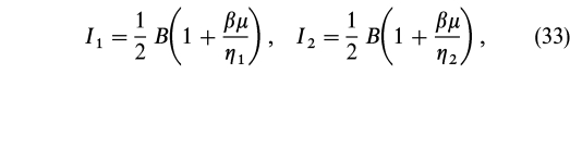
where it has been assumed that the η terms are constant with depth. The Stokes parameters in the Cartesian basis are calculated from the transformation
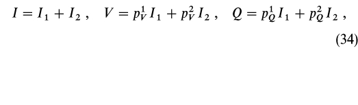
where the four coefficients p1Q,p2Q,p1V,p2V specify the polarization of the normal modes. For an ionized plasma, the normal modes are orthogonal provided ω≫νe, where νe is the electron ion collision frequency. For this case (Kaminker et al. 1982)
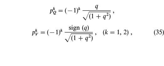
where

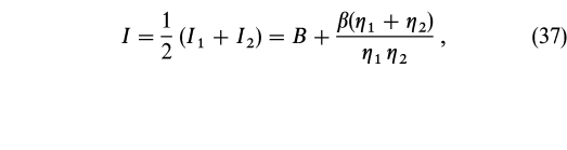
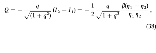
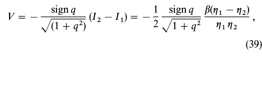

These solutions illustrate the following: (a) a temperature gradient is required to produce polarization in an optically thick atmosphere; (b) the amount of polarization is proportional to the difference η1 - η2 between the opacity ratios of the two normal modes; (c) Q can change sign across the boundary η2/η1 = 1 and result in a rotation in the linear polarization angle by 90°.
For ω/ωC≫1, the continuous opacity takes the form

for a variety of commonly occurring processes such as magneto‐bremsstrahlung and electron scattering (γ = 4) (Gnedin & Pavlov 1974). For these cases the above solution yields
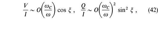
which is the commonly used low‐field expression.
However, given the different sources of magnetic dichroism and birefringence in the atmosphere, and the changing physical conditions with depth, normal modes can be defined only locally, and in general they may not be orthogonal. Thus, when bound electrons are present, deviations from orthogonality will occur particularly near spectral lines. The normal‐mode approach therefore offers no computational economies in the solution of the transfer equations in the general case.
Martin & Wickramasinghe (1982) used the full Stokes formulation to show that provided the Faraday terms (the ρ terms) dominate over the dichroism terms (the η terms in eq. [16]), and the Faraday terms are those appropriate to a fully ionized plasma, equation (37) is recovered. However, if other sources of dichroism are present, it will be necessary to carry out the solution of the full set of transfer equations.
5.4.1. The Rotation of the Continuum Linear Polarization Angle
Some strongly polarized white dwarfs such as Grw +70°8247 and GD 229 show a flip in the polarization angle as the wavelength increases above some critical wavelength λcrit. Typically, the polarization angle flips through 90°, and the change occurs over a narrow wavelength range. From the data for Grw +70°8247 shown in Figure 11, the rotation of the continuum polarization angle occurs near λcrit = 5500 Å.
The observed phenomenon is related to the change in the absorption, scattering and transport properties of a magnetic atmosphere as one crosses from the low‐field ω/ωC≫1 to the high‐field ω/ωC≪1 regime. Classically, in the low‐field limit, a free electron will absorb or scatter as would a circular σ+ oscillator rotating in a plane perpendicular to the magnetic field. In the high‐field limit, on the other hand, the electron will be behave as a linear π oscillator oriented parallel to the field. The polarization angle will rotate at the frequency at which the absorption (or scattering) properties change from being dominated by the extraordinary mode (η1>η2) to the ordinary normal mode (η1<η2). For magneto‐bremsstrahlung opacity (Martin & Wickramasinghe 1986) and electron scattering opacity (Whitney 1991a), the rotation occurs at ωcrit = 3 ωC.
GD 229 has a low level of circular polarization longward of λcrit, while Grw +70°8247 exhibits the opposite behavior. On the above scenario, the optical emission in GD 229 must be in the long‐wavelength tail of the cyclotron fundamental, while in Grw +70°8247 the opposite must hold. Barring effects due to field structure, one would expect the mean field of GD 229 to be about 3 times larger than Grw +70°8247 (cf. the observed value of ∼2 from Zeeman line identifications).
The interpretation of polarization angle data is complicated by the presence of field spread. Martin & Wickramasinghe (1986) and subsequently Jordan (1989) used the classical results of Pacholcyzk (1976) for magneto‐bremsstrahlung opacity and the associated Faraday terms and showed that a rotation in the polarization angle would survive even in the presence of dipole field broadening as in the case of Grw +70°8247, but only for special viewing angles. Whitney (1991b) used Monte Carlo methods to solve the transfer equations in a pure scattering atmosphere allowing for field spread in a dipolar field and reached similar conclusions. Dittman & Wickramasinghe (1999) reinvestigated this problem for an atmosphere with both scattering and magneto‐bremsstrahlung opacity using a robust numerical method for the solution of the full transfer equations and confirmed the above results for more general field distributions. However, it still needs to be demonstrated that the inclusion of magnetic dichroism by bound‐free edges will not destroy this general picture.
6. MAGNETIC WHITE DWARFS IN INTERACTING BINARY SYSTEMS
The AM Hers provide an excellent opportunity for determining magnetic fields and field structure in a wider sample of MWDs, often using methods unavailable for single MWDs. Phase‐dependent Zeeman spectroscopy and polarimetry can in principle be carried out for all AM Hers since the rotation periods are known (typically a few hours), and the presence of shock emission enables the magnetic properties of localized regions on the white dwarf surface to be studied through cyclotron spectroscopy—a method which, as we have already seen, is ineffective in isolated MWDs.
A typical CV first comes into contact after the common envelope phase of evolution at orbital periods of ∼hours to ∼day and evolves toward shorter orbital periods, transferring matter from the companion star to the WD until the period minimum (Porb∼80 minutes) is reached. The orbital evolution is driven by angular momentum loss due to a combination of magnetic braking in a stellar wind emanating from the late‐type secondary and gravitational radiation on a timescale of ∼109 yr (Lamb 1988). The resulting orbital evolution is punctuated by nova explosions, and it is unclear from theoretical considerations whether the mass of the WD would increase or stay nearly the same. The role played by magnetic fields in this process is also essentially unexplored. For instance, if mass is lost or gained during evolution, one may expect the magnetic field of the WD also to evolve with period. The reader is referred to Warner (1995) for a comprehensive account of the properties of CVs.
6.1. The Basic Model
We show in Figure 29 and Figure 30 the main features of the basic model which has been developed for the AM Herculis systems. This picture is based on a variety of considerations based on X‐ray observations (e.g., Beuermann 1998), stream mappings and Doppler tomography (e.g., Marsh & Horne 1987; Hakala 1995; Schwope, Mantel, & Horne 1997a), and modeling of the continuum and emission‐line radiation from magnetically confined accretion funnels (Ferrario & Wehrse 1999) and polarized emission from shocks (e.g., Ferrario & Wickramasinghe 1990; Potter, Cropper, & Hakala 1998).
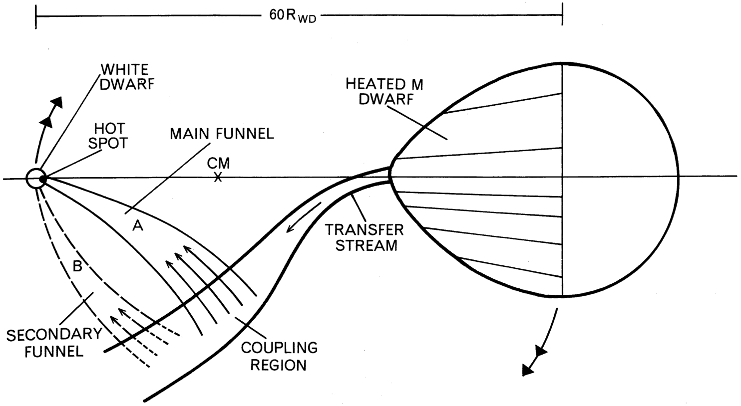
Fig. 29.— A schematic representation of the accretion pattern in AM Hers
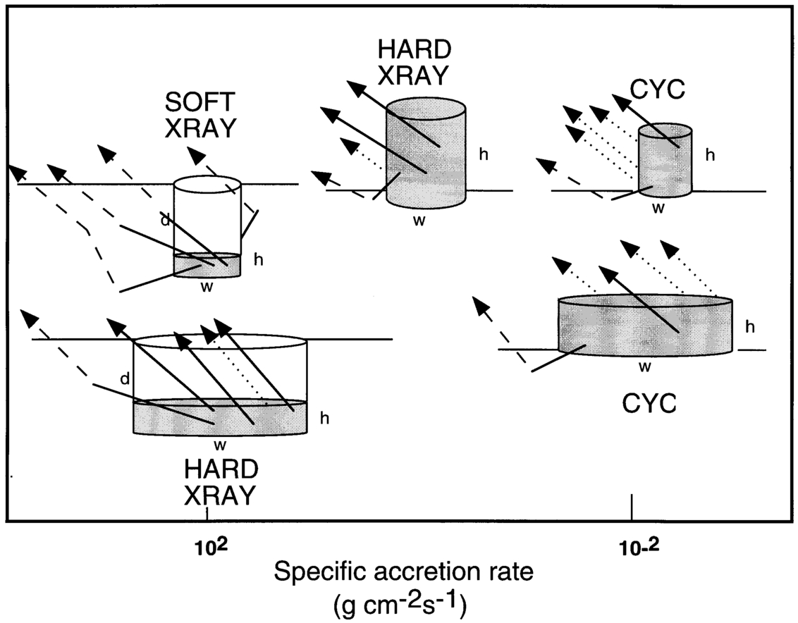
Fig. 30.— A schematic representation of the expected components in a typical shock region in AM Hers as a function of the specific accretion rate
The mass transfer stream first free falls toward the MWD following a ballistic trajectory. The gas in this region is heated by X‐rays or softer radiation related to the accretion shock and makes a major contribution to the emission‐line spectrum. The magnetic pressure (∝R-6 for a dipole), which increases rapidly as the MWD is approached, soon begins to dominate the flow. In a transition region, referred to as the coupling region, the radial component of the velocity is reduced and the flow acquires toroidal and then poloidal velocity components as it couples onto field lines and free falls once again toward the surface of the white dwarf, but this time in magnetically confined funnels. The coupling region and the accretion funnels are also heated by accretion energy and make significant contributions to the continuum and the line emission (Ferrario & Wehrse 1999). The least understood of the three regions is the coupling region, although its radial thickness is expected to be small (ΔRcoup/Rcoup≪1).
6.1.1. Shock Structure
The radiation from the AM Hers is dominated by shock related emission in both the optical and the X‐ray wave bands. The interpretation of the cyclotron and X‐ray spectra which allows the properties of the MWD to be studied depends on the physics of the shock. We therefore present a brief review of the relevant theory.
Consider the accretion flow along an accretion funnel. The accretion luminosity per unit area is
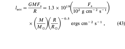
where Fs is the specific accretion rate. For comparison, the Eddington luminosity per unit area is
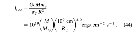
Observed systems show 10-4≲lacc/lEdd∼1.
In a strong shock, the velocity is reduced from the free‐fall value vff by a factor of 4, and the density is increased by the same factor. The adiabatic shock temperature (Ts = 3GMmpμ/8kR) for normal composition is
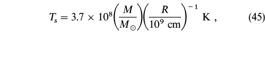
and the postshock electron density is
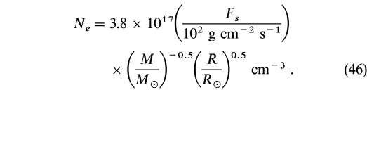
The ions which carry the bulk of the energy of the infalling gas will first form an ion shock of width hion∼0.25vfftii, where tii is the ion‐ion collision timescale. The shocked ions transfer their energy to the electrons through Coulomb collisions, and the gas cools by bremsstrahlung and cyclotron radiation as it settles on the white dwarf surface. The properties of the postshock region depend on tii, and the timescales tie for ions to transfer energy to electrons, and tcool for electrons to cool. Usually, the electron temperature Te differs from the ion temperature Ti, and both vary with height in the shock (Lamb & Masters 1979; Imamura et al. 1987; Wu & Chanmugam 1990).
Bremsstrahlung cooling dominates at low fields and/or high specific accretion rates, and cyclotron cooling dominates at high fields and/or low specific accretion rates (Lamb & Masters 1979). When bremsstrahlung is the dominant cooling mechanism (tii≪tie≪tcool), Ti = Te to a good approximation. This is known as "the single‐fluid" approximation. In this regime, Te = Ti = Ts, and the shock height 0.25vfftbr is given by
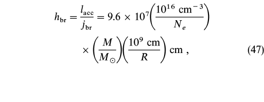
where jbr = 2 × 10-27N2eT1/2e ergs cm−3 s−1 is the bremsstrahlung emissivity per unit volume.
When cyclotron cooling is dominant, the electrons cool faster than they can be heated by collisions with ions (tcool≪tie), and the electrons and ions no longer have the same temperature. This regime is known as "the two‐fluid" regime. The cyclotron cooling rate depends rather sensitively on the optical depth to cyclotron emission and cannot be easily parametrized except for special geometries. Typically, when cyclotron cooling dominates hcyc≪hbr.
There is another regime which occurs at even lower specific accretion rates or equivalently very high magnetic fields when tcool≪tii. The energy of the ions is then communicated to the atmospheric particles over the distance of a mean free path, and a shock does not form. In this "nonhydrodynamic" regime, the shock solution degenerates into a bombardment‐type solution (Kuijpers & Pringle 1982; Thompson & Cawthorne 1987).
The shocks in AM Hers appear to be in the difficult two‐fluid or bombardment regimes—difficult, because a proper treatment of shock structure will ultimately require radiative transfer and three‐dimensional geometrical structure to be considered, and this has not been achieved as yet. Calculations which cover all the above mass transfer regimes in the one‐dimensional plane‐parallel approximation have been published by Woelk & Beuermann (1992, 1993) and are the most detailed presently available. These calculations do not include thermal conduction, so that the shock precursor has not been modeled.
6.1.2. The Clumpy Accretion Model
If the accretion energy is released entirely in shocks, the primary sources of shock radiation will be 10–30 keV bremsstrahlung hard X‐ray emission and optical cyclotron emission. The soft X‐ray luminosity will then arise as reprocessed secondary emission from the surface of the WD with a luminosity which cannot exceed that of the primary source[Lsoft∼ 1 / 2(Lhard + Lcyc)]. In many systems, the ratio of the luminosities of the soft and the hard X‐ray components Lsoft/Lhard∼10–100, contradicting expectations from the simple shock model (the "soft X‐ray mystery"; e.g., see Heise et al. 1985; Ramsay et al. 1994).
Kuijpers & Pringle (1982) first noted that if the flow is clumpy, material may penetrate deep into the white dwarf photosphere. The accretion energy carried by the clumps will then be thermalized and radiated at a temperature
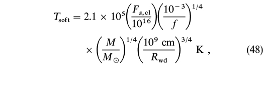
where f is the fractional area of the white dwarf covered by the clumps and Fs,cl is a mean specific accretion rate for this component. The clumps originate due to instabilities which develop in the stream‐magnetosphere interaction region (Lamb 1988; Stockman & Schmidt 1996), or the flow may be clumpy right at the source where it originates, namely, the Lagrangian nozzle, due to the effects of irradiation (King 1989). The clumpy accretion model provided an elegant solution to the soft X‐ray mystery which plagued the field for many years, but it also introduced an additional degree of complexity into the problem.
A more realistic method of looking at clumpy accretion may be in terms of "buried shocks," a notion introduced by Kuijpers & Pringle (1982) and developed further by Beuermann (1988) and Stockman (1988) at the Vatican Conference. They noted that at sufficiently high specific accretion rates (∼102 g s−1), the ram pressure of the flow would bury the shock below the stellar photosphere and the shock emission will be thermalized in the photosphere. As the specific accretion rate is reduced, the shock will rise above the photosphere, first as a bremsstrahlung‐dominated shock, then as a cyclotron cooling–dominated shock, and will eventually collapse back to the surface as the bombardment regime is reached. Depending on the lateral width of the shock w and the depth of burial d, the radiation could appear either totally or partially reprocessed. This scenario is illustrated in Figure 30.
Each accretion region on the MWD surface will have a distribution of Fs, perhaps with the flow being in the form of discrete accretion filaments. Since the high‐density filaments (the clumps) will carry most of the mass and accretion energy, and the resulting shocks will be buried and thermalized, it is likely that they will dominate the soft X‐ray emission. The lower density regions will give rise to hard X‐rays and cyclotron emission.
Observations in the X‐ray band generally support this picture. In the soft X‐ray band (≲0.4 keV) flare‐type activity is often seen on timescales of minutes to tens of minutes, much shorter than the orbital period (Ramsay, Cropper, & Mason 1996). This is very likely to be related to the entry of discrete clumps into the WD photosphere. At higher energies, on the other hand, the modulation is at the orbital period, suggesting that the lower density filaments may be behaving essentially like a fluid flow forming a persistent standoff shock.
The two poles generally have distinct X‐ray characteristics. One of the poles tends to emit mainly in the soft X‐rays, and the other, mainly in hard X‐rays. There is also strong empirical evidence that the magnetic field plays a crucial role in the cooling of the electrons. In general, poles with a higher field and a lower accretion rate exhibit much softer X‐ray spectra (Ramsay et al. 1994). As will be shown in the following sections, the optical properties of the two poles tend also to be quite distinct.
6.2. Magnetic Field Determinations
6.2.1. Cyclotron Emission: Theoretical Considerations
The first field determination in an AM Her came with the discovery by Visvanathan & Wickramasinghe (1979) of resolvable high harmonic cyclotron lines in VV Puppis. The field of 3 × 10⁷ G deduced from cyclotron spectroscopy for this star was somewhat lower than anticipated from the high level of circular polarization (typically 10%–50%) seen in these systems by analogy with the isolated MWDs.
Optical cyclotron spectroscopy has since proven to be the main method of determining magnetic fields of MWDs in these systems. At the electron temperatures expected in the shock (10–30 KeV), thermal Doppler broadening (∼1000 Å) is expected to have an impact on the spectrum, but high harmonic cyclotron features can nevertheless be seen resolved provided the shock is viewed nearly obliquely to the field direction for the following reasons.
A single electron radiating in a magnetic field B contributes radiation at the frequencies (Bekefei 1966)

where β∥ is the velocity component parallel to the field in speed of light units, γ = 1/ 1 - β2, and ωC/γ is the fundamental cyclotron frequency for a relativistic electron of mass γme. What we observe at a given harmonic number n is a suitable average of the above expression which allows for velocity spread in a relativistic Maxwellian distribution. The radiation at high harmonics (high n) comes preferentially from the high‐energy (high γ) electrons in the Maxwellian distribution, and these harmonics therefore develop a low‐frequency tail, which is a characteristic of cyclotron emission.
We note that the term β∥ cos θ in the denominator, which arises from the Doppler effect, vanishes at θ = 90° but becomes increasingly more important as θ approaches zero. On the other hand, the broadening which arises from the spread in γ in the velocity distribution ("relativistic mass broadening") is independent of the viewing angle θ. At θ = 90°, when the Doppler term makes no contribution, relativistic mass broadening dominates. This broadening increases with temperature, and it is only at temperatures of ∼50 KeV, well above what is expected in shocks in normal mass WDs, that the relativistic mass broadening term will render the cyclotron lines undetectable even at θ = 90°. The cyclotron lines in the AM Hers are in fact seen only when the shocks are viewed at large angles to the field direction when the Doppler effect is at a minimum. The intensity is strongest at the fundamental and declines rapidly at higher harmonic numbers, the rate of decline depending on temperature. Approximately, Iω∝ωp, where p = -8, −5, −3, and −1.4 for Te = 10, 20, 50, and 100 keV, respectively, for emission perpendicular to the field.
The emission is also strongly polarized and angle dependent, being preferentially beamed perpendicular to the magnetic field at high harmonics. The beamwidth is given approximately by
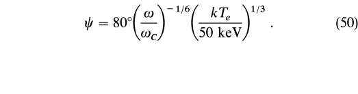
The polarization changes from circular along the field to linear perpendicular to the field as for a σ+ component (Chanmugam & Dulk 1981; Meggitt & Wickramasinghe 1982) and can again be understood by considering the projection of the acceleration vector onto the plane of the sky. The beaming and polarization characteristics are shown schematically in Figure 31.
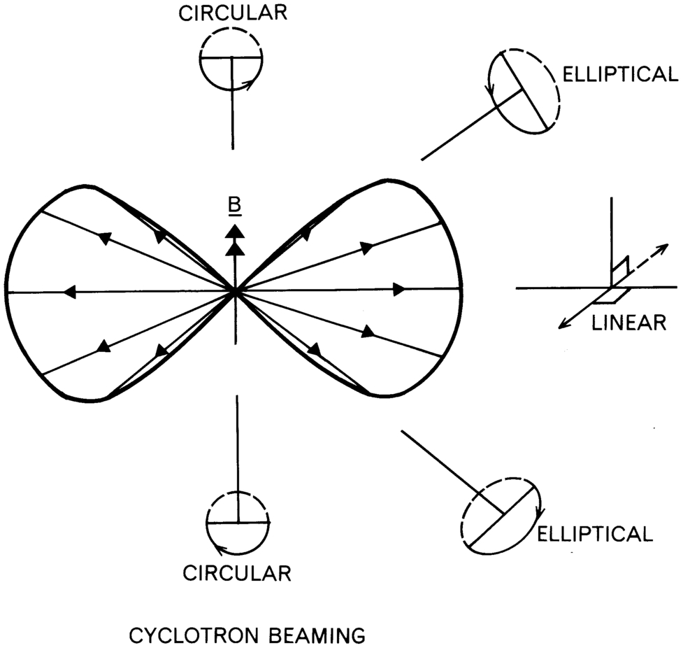
Fig. 31.— A schematic view of the beaming and polarization properties of high harmonic cyclotron radiation
The polarized transfer equations which yield the cyclotron spectrum are as given in § 5.1. The opacities now take the form
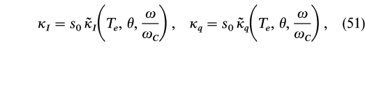
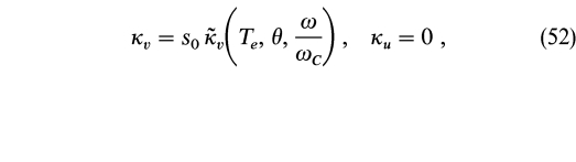
where s0 = ω2p/cωC and ωP is the plasma frequency. Expression for κ ˜I, κ ˜q, κ ˜v can be found in Meggitt & Wickramasinghe (1982). An alternative approach is to use the normal‐mode formulation in the limit of large Faraday rotation (Chanmugam & Dulk 1981).
It follows from the above scaling that for pure cyclotron opacity (∝Ne), the emergent spectrum depends only on Te, θ,ω/ωC and the optical depth parameter
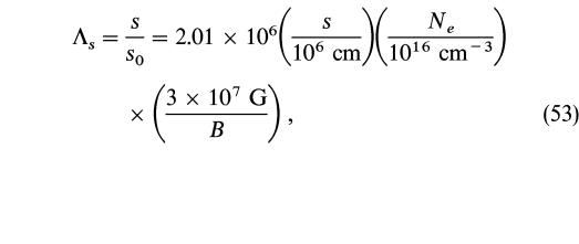
where s is a characteristic path length through the postshock region. The optical depth τκ = Λs κ ˜I(Te, θ,ω/ωC), and Λs is approximately equal to the optical depth at the cyclotron fundamental for viewing at an angle θ = 90° to the field direction.
Away from the cyclotron resonance peaks, and at high harmonics, electron‐ion collisions become important in determining the opacity. As a first approximation, these can be taken into account by adding to the collisionless cyclotron opacity, the magneto‐bremsstrahlung opacity. Since the latter is ∝N2e, the absolute value of the density now enters the calculations, and a simple scaling is no longer possible. In practice, collisional effects are relatively more important in low‐field and low‐temperature shocks (Wickramasinghe 1988).
We show in Figure 32 a selected set of theoretical calculations of cyclotron lines for a viewing angle θ = 90°. These spectra serve to illustrate various points. The spectrum resulting from pure thermal cyclotron emission is characterized by a cyclotron "continuum" (the region between harmonics) modulated by resolvable cyclotron lines. The "continuum" consists of an optically thick Rayleigh‐Jeans tail Iω∝ω2 at long wavelengths and a power‐law spectrum Iω∝ω-p modulated by cyclotron lines at shorter wavelengths. The Rayleigh‐Jeans–type behavior simply reflects the fact that the emission is optically thick at the harmonic peaks at low harmonic numbers. Note in particular the flat‐topped profiles of these harmonics. It is only at high harmonic numbers ω/ωC≫1, when the opacity drops and the shock becomes marginally optically thin or optically thin, that discernible harmonic structure can be seen modulating the cyclotron continuum (see Meggitt & Wickramasinghe 1982 and Wickramasinghe & Meggitt 1985 for tabulated results). The harmonic number n* at which the emission changes from being optically thick to thin can be determined by the frequency at which the power‐law index of the cyclotron continuum slope changes sign and is strongly dependent on the optical depth parameter Λ. The relationship n*(Λ) has been presented graphically in Wickramasinghe (1988) and can be used in conjunction with observations to estimate the optical depth parameter of the postshock region.
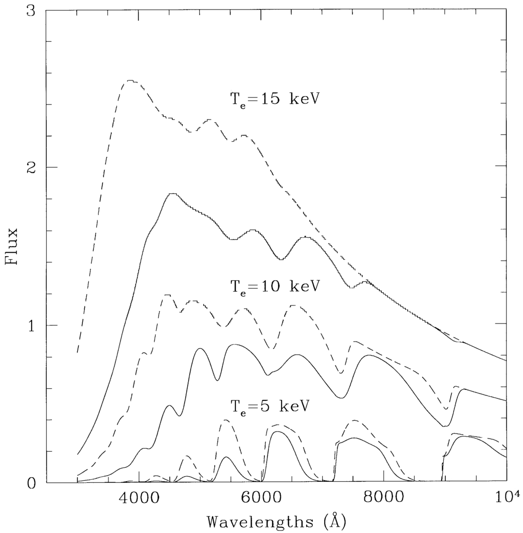
Fig. 32.— Theoretical cyclotron spectra (Iν) as a function of electron temperature Te for a viewing angle θ = 90°. The solid and dashed curves are for optical depth parameter Λ = 2 × 10⁵ and Λ = 106, respectively. The magnetic field B = 30 MG.
The cyclotron emission profiles have a characteristic asymmetric profile with an extended red wing arising from the high‐energy tail of the Maxwell‐Boltzmann distribution. The asymmetry persists as the temperature increases until the features are broadened beyond recognition and is an excellent indicator of electron temperature.
6.2.2. Cyclotron Spectroscopy of AM Hers
Depending on the state of activity (the mass transfer rate) of the system, the spectral appearance could be quite different. In a very low state, the continuum energy distribution is mainly dominated by the stellar photospheres, and the heated photosphere (due to X‐rays from previous high states) gives rise to line emission (a narrow component) (Schmidt et al. 1996b). Only a few systems are seen in this state. At a somewhat higher mass transfer rate, in addition to the narrow component, accretion streams begin to dominate the line emission, contributing a structured broad component. In addition, cyclotron emission from one shock may contribute to the optical emission dominating at some phases showing a single sequence of cyclotron lines. When the mass transfer rate increases even further, two sequences of cyclotron lines may be seen one from each pole, and the sequences may overlap at some phases. The visibility of the shocks will of course depend on viewing geometry. The orbital inclination i and the field structure and orientation therefore become important parameters in the modeling procedures. Once successive harmonics have been identified, an estimate of the field can be obtained from
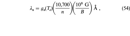
where gn(Te) is a slowly varying function of n at a given temperature and has been tabulated in Wickramasinghe (1988). For Te≲10 keV one can assume gn(Te)∼1 as a first approximation.
We show in Figure 33 (top panel) the bright‐ and faint‐phase spectra of VV Puppis in its 1979 low state of accretion when cyclotron harmonics were first discovered (Visvanathan & Wickramasinghe 1979). The magnetic field strength deduced from the spacing of the cyclotron humps in the bright‐phase spectrum corresponds to 32 MG. Note that there are no cyclotron harmonic features in the faint‐phase spectrum, that is, when the main cyclotron emission region becomes hidden by the body of the white dwarf. The same system was seen to exhibit quite a different behavior in its 1989 high state of accretion. During this state, accretion occurred on to both poles, and the faint‐phase spectrum (Fig. 33, lower panel) also showed cyclotron harmonics. The features are now more widely separated in frequency, indicating a somewhat higher field of 56 MG (Wickramasinghe, Ferrario, & Bailey 1989), which is the field at the second pole. Note that the higher field pole exhibits cyclotron lines that are more symmetric. The plasma which emits cyclotron lines in this region is more strongly cooled, and as a result relativistic mass broadening is less important (§ 6.2.1).
Fig. 33.— Top: Bright‐ and faint‐phase spectra of VV Puppis in its 1979 low state of accretion (from Visvanathan & Wickramasinghe 1979). The bright‐phase spectrum shows broad cyclotron emission features centered at 6300, 5500, 4800, and 4100 Å corresponding to harmonic numbers 5, 6, 7, and 8, respectively, at a field of 32 MG. Bottom: Faint‐phase spectrum of VV Puppis in its 1989 high state of accretion (from Wickramasinghe et al. 1989) showing a different sequence of cyclotron harmonics this time centered at 6700, 5100, and 4200 Å corresponding to harmonic numbers 3, 4, and 5 at a field of 56 MG. These lines come from the second pole. Copyright Nature and Astrophysical Journal, reproduced with permission.
The above classical behavior is observed in many other systems such as UZ For (Beuermann, Thomas, & Schwope 1988; Ferrario et al. 1989) QS Tel (Ferrario et al. 1994; Schwope et al. 1995b), and DP Leo (Wickramasinghe & Cropper 1993), where cyclotron lines have been detected from both poles. A significant result, common to all cyclotron models, is the low value deduced empirically for the optical depth parameter of the region giving rise to optical cyclotron emission (Λ∼102–105), compared with the theoretical value
expected for a bremsstrahlung‐dominated shock (eqs. [47] and [53]) independently of the accretion rate. This result supports the view that the optical cyclotron radiation originates mainly from strongly cyclotron cooled shock elements with low specific accretion rates consistent with scenario outlined in § 6.2.1.
In lower field systems, the wavelength of the cyclotron peak will move into the IR, if the accretion rate and hence n*(Λ) is the same. Four AM Herculis systems have been studied spectroscopically in the near‐IR. They all show prominent cyclotron features. These are AM Herculis itself, observed and modeled by Bailey, Ferrario, & Wickramasinghe (1991), who deduced a magnetic field of 14 MG; ST LMi, for which Ferrario, Bailey, & Wickramasinghe (1993) calculated a field of 12 MG; BL Hyi, which was fitted using a field of 23 MG (Ferrario, Bailey, & Wickramasinghe 1996), and EF Eri, which was modeled with a field of 17–21 MG (Ferrario et al. 1996). None of these systems shows resolvable cyclotron features in the optical band. The IR spectrum of ST LMi and the cyclotron model fit are shown in Figure 34.
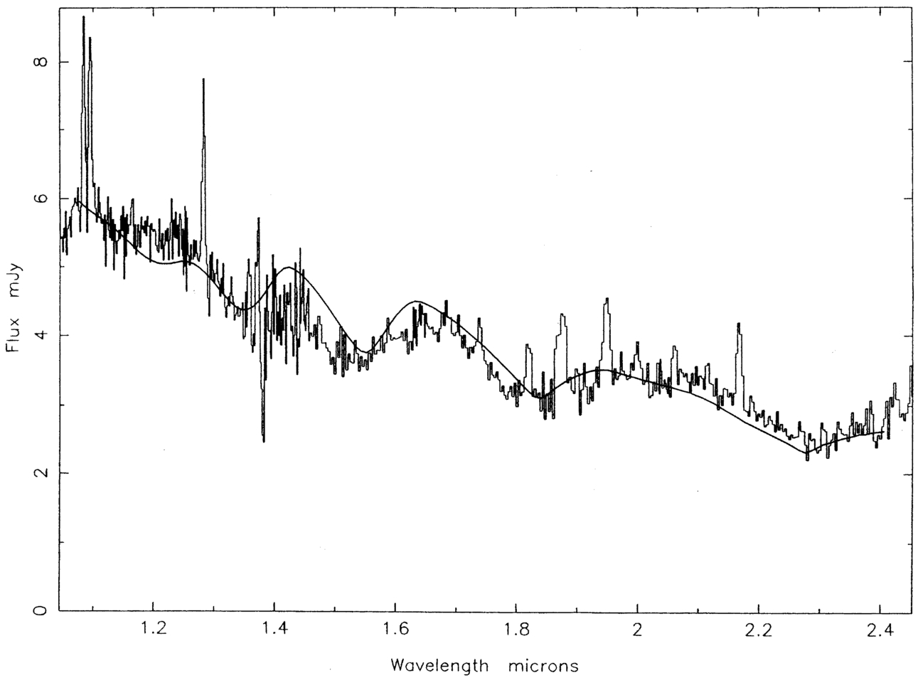
Fig. 34.— Bright‐phase spectrum of ST LMi obtained by Ferrario et al. (1993). The solid line is their best cyclotron harmonic fit to the data. Copyright Monthly Notices of the Royal Astronomical Society, reproduced with permission.
High‐field systems appear to be very rare. There is only one system, AR UMa, which truly belongs to this class, and it was discovered only recently (Schmidt et al. 1996b). The system was detected as a transient soft X‐ray source (1ES 1113+432) from the Einstein Slew Survey and was later discovered to be a high‐field MWD (B∼230 MG) by Zeeman spectroscopy (Schmidt et al. 1996b). In the low state, the stellar photospheres dominate the light, and the polarization is magneto‐bremsstrahlung from the white dwarf photosphere V/I = 2.2%–4.3%; it varies with the orbital period as the white dwarf spins. In the high state of accretion, continuum circular polarization is essentially absent (V/I = 0.52% ± 0.18%) because there is additional diluting light presumably from the funnels, the heated white dwarf, optically thick cyclotron around the fundamental, and the heated secondary star (Schmidt et al. 1996b). The system has so far been observed mainly in a low state with brief periods of high accretion (Schmidt et al. 1999b).
6.2.3. Zeeman Spectroscopy of AM Hers
The most powerful method for investigating field structure is Zeeman spectroscopy and spectropolarimetry of the underlying magnetic white dwarf during a low state when the photospheric emission from the white dwarf dominates over the radiation from the accretion shocks and the accretion stream. Phase‐resolved Zeeman spectroscopy can be used to place strong constraints on the surface‐averaged field as well as on field structure, as was shown by Wickramasinghe & Martin (1985; see also Latham, Liebert, & Steiner 1981). Unfortunately, this information is available only for a few systems. Phase‐resolved spectropolarimetry over a spin cycle is required to firmly tie down field structure. Potentially, the AM Her sample offers a much larger sample than isolated magnetic white dwarfs for such a study, but because of their intrinsic faintness may require the use of 8 m class telescopes.
Zeeman spectroscopy of AM Herculis (Latham et al. 1981; Wickramasinghe & Martin 1985), MR Ser (Schwope et al. 1993b), and 1H 1752+081 (Ferrario et al. 1995) has provided unambiguous evidence for field distributions which differ from a centered dipole. As a first approximation, the field distributions can be modeled by dipoles which are offset from the center of the star by 0.1–0.3 of the white dwarf radius along the dipole axis.
The observations and models for AM Herculis are shown in Figure 35. The data show the maximum field broadening at phase 0.97 (the phase of the linear pulse), when we expect the main cyclotron emission region to be viewed nearly orthogonal to the field direction. The centered dipole model, on the other hand, predicts the minimum field broadening at this phase (dipole viewed close to equator‐on) and the maximum field broadening at the opposite phase (pole‐on viewing), contrary to observations. However, the data are well fitted by the offset dipole model at both phases.
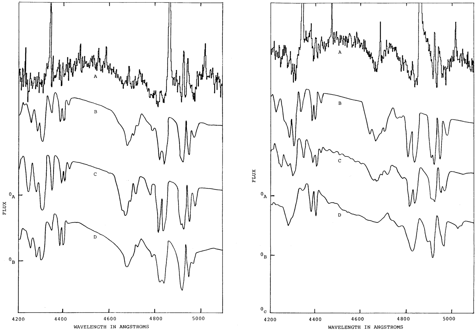
Fig. 35.— Observed (top spectra, marked A; Latham et al. 1981) and theoretical spectra for AM Herculis (Wickramasinghe & Martin 1985) at two different (opposite) phases corresponding to the two hemispheres of the star. Left panel: Zeeman modeling of AM Her at phase 0.97. Right panel: Zeeman modeling of AM Her at phase 0.55. Models B correspond to a dipole offset by −0.17 radii along the dipole axis and have Bp = 22 MG; models C correspond to a centered quadrupole with Bp = 26 MG; and models D correspond to a centered dipole with Bp = 22 MG. Copyright Monthly Notices of the Royal Astronomical Society, reproduced with permission.
Observations of MR Ser (Schwope et al. 1993b) have yielded a similar result, but with a dipole that is even more strongly offset (az = 0.3) as shown in Figure 36.
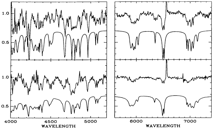
Fig. 36.— Observations of the underlying MWD in MR Ser obtained at two opposite phases compared with a model with an offset dipole model with Bd = 56 MG and az = 0.3. The spectra in the upper panel (phase 0.0) show lines that are much more strongly field broadened than those in the lower panel (phase 0.5). Copyright Astronomy and Astrophysics, reproduced with permission.
AM Hers have also been observed when photospheric Zeeman lines and cyclotron lines are simultaneously visible. This usually occurs when the systems are in an intermediate state of activity so that the cyclotron component is strong but does not overwhelm the contribution from the photosphere of the white dwarf. The first system to show this behavior was V834 Cen (Ferrario et al. 1992). In this system we see Zeeman‐split Hβ and Hα in the blue spectral region and cyclotron lines in the red part of the spectrum (Fig. 37). A more recent similar example is 1RXS J012851.9−233931 (Schwope, Schwarz, & Greiner 1999). The data of these two systems and models of the two components are shown in Figure 37.
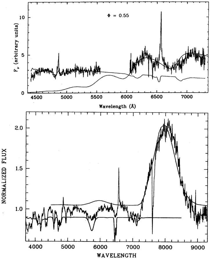
Fig. 37.— Top panel: Observations of V834 Cen showing both photospheric Zeeman (Bp = 31 MG, az = -0.1) and cyclotron lines (Bc = 23 ± 1 MG) obtained at phase 0.55 compared with models from Ferrario et al. (1992). Bottom panel: Observations of 1RXS J012851.9−233931 showing a strong cyclotron line in the red (Bc = 45 ± 1 MG) and a photospheric Zeeman spectrum with 〈B〉 = 36 ± 1 MG (Schwope et al. 1999). Copyright Monthly Notices of the Royal Astronomical Society and Astronomy and Astrophysics, reproduced with permission.
6.2.4. Halo Zeeman Lines
Another method of measuring magnetic fields in the AM Herculis–type systems is through the detection of "halo" Zeeman features of hydrogen. These features were first detected in absorption during a high state of V834 Cen (Wickramasinghe, Tuohy, & Visvanathan 1987) at phases when cyclotron emission from the shock dominated in the optical band (Fig. 38). The halo Zeeman lines are seen only when the cyclotron continuum is strongest (i.e., when the shock is viewed nearly perpendicular to the field direction) and disappear at other phases. They can therefore readily be distinguished from photospheric Zeeman lines (cf. the spectrum of V834 Cen in Fig. 37 obtained when the system was somewhat fainter).
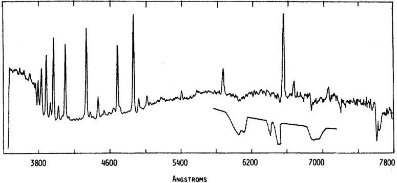
Fig. 38.— Observations of V834 Cen during a high state showing a Zeeman‐split Hα line against a strongly modulated cyclotron continuum. The field strength BH = 23 MG deduced for the halo is very close to the cyclotron field strength Bc = 23 MG (Wickramasinghe et al. 1987). The "halo" lines are formed in cool gas very close to the accretion shock and are seen only at some phases.
The halo Zeeman lines are attributed to free‐falling cool material in the vicinity of the shock (Wickramasinghe et al. 1987). Achilleos, Wickramasinghe, & Wu (1992b) modeled the thermal structure of this gas and showed that the required temperatures could be provided by hard X‐ray heating due to radiation from the shock. In the context of the clumpy accretion model, the most likely location of the material giving rise to the halo Zeeman lines would be the dense gas in the accretion filaments which form the buried shocks. The clumpiness of the flow may therefore play a role in determining the presence of absence of halo lines.
There is generally very close agreement between fields determined using cyclotron lines and halo Zeeman features, and in the absence of cyclotron line field determinations, the halo field can be taken to be the field strength at the accretion shock to within a few percent.
6.2.5. Magnetic Fields and Field Structure
We summarize in Table 2 the field determinations for those AM Hers for which magnetic field determinations have been possible on the basis of cyclotron and/or Zeeman spectroscopy. Terms Bc1 and Bc2 are the cyclotron fields at the two poles, and 〈B〉 is the mean field from photospheric Zeeman lines. BH is the field determined from halo Zeeman lines. Table 2 shows that the field strengths at the two accreting poles (from cyclotron or halo Zeeman lines) typically differ by a factor of about 1.4–2 in all systems for which suitable data are available. As a first approximation, the observations may be interpreted in terms of a simplistic model in which accretion occurs along closed field lines onto opposite poles in a dipolar or to more poles in a multipolar field structure (see Wickramasinghe 1988 for a basic review of two‐pole emission). If we adopt the closed field line model, this implies that the disparity in field strengths is caused mainly by the noncentered dipolar nature of the field distribution. In the three systems where the Zeeman spectrum of the underlying photosphere has been modeled by offset dipoles, the polar field strengths are similar to those found for the accretion shock (s) from cyclotron lines, which is strong independent support for the closed field line model.
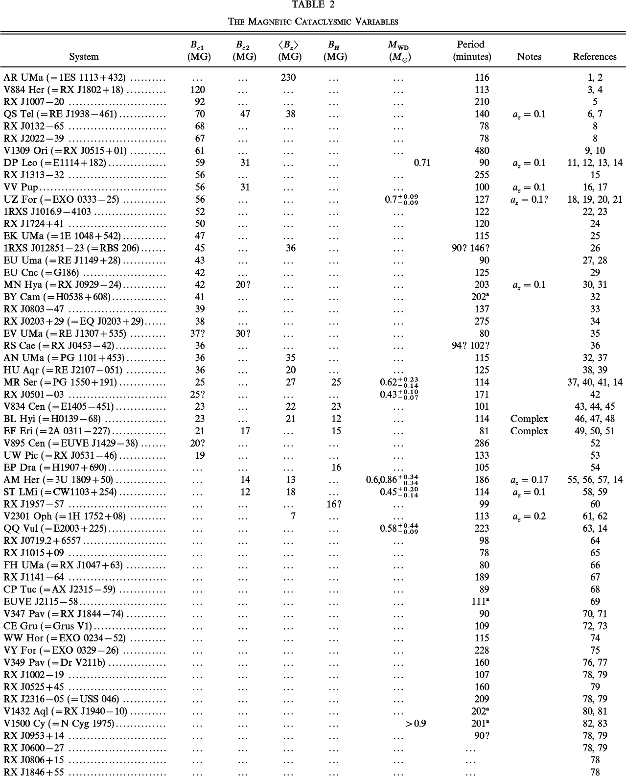 |
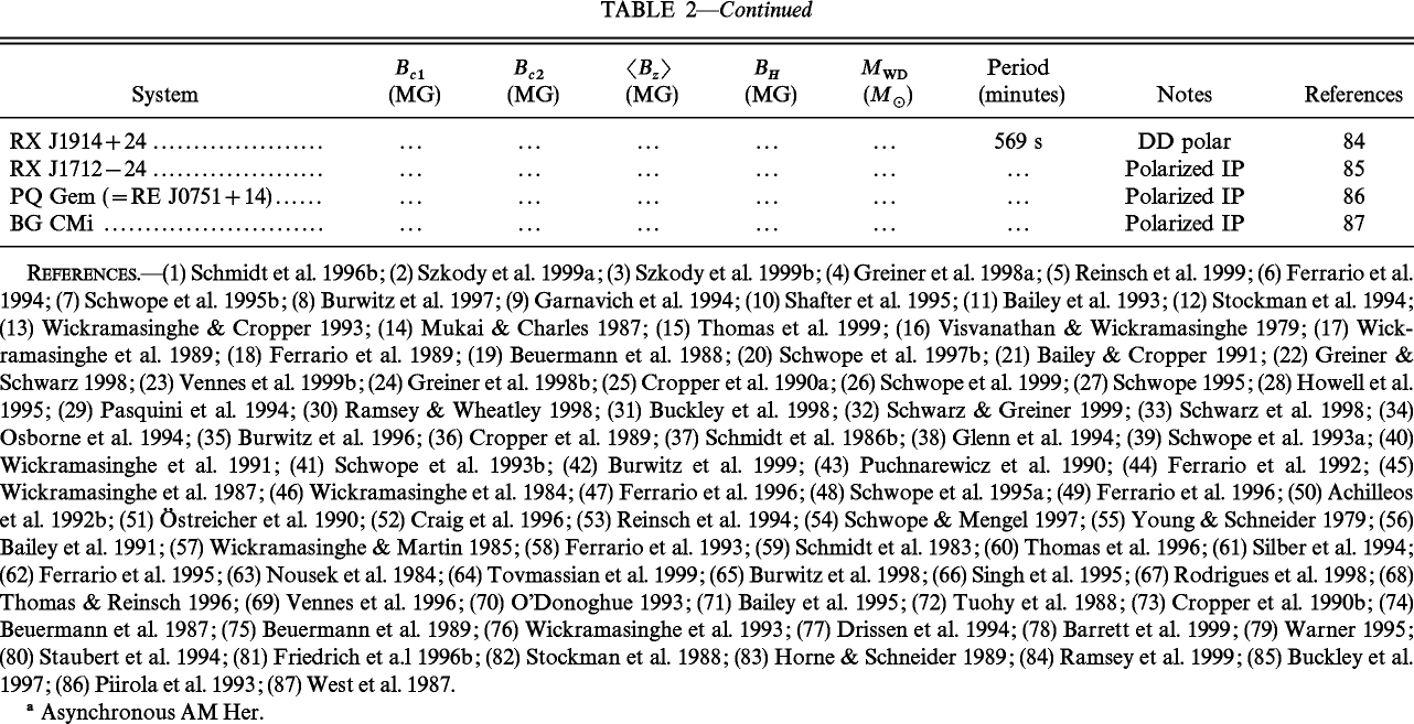 |
There is also evidence for even more complex field structure also in the AM Hers. The possibility of dominant quadrupolar field components was first proposed by Meggitt & Wickramasinghe 1989) for EF Eri based on an interpretation of linear polarization observations. More recently, Schwope, Beuermann, & Jordan (1995a) have argued for a strong quadrupolar component in BL Hyi from Zeeman spectroscopy, and Mason et al. (1995) have presented different lines of evidence to argue for a dominant quadrupolar component in the slightly asynchronous AM Herculis system BY Cam.
The observations generally show that in all but one of the well‐studied systems, the more strongly accreting magnetic pole points (to within ∼±45°) toward the secondary star. In most, but not all, systems this pole leads the secondary (Wickramasinghe & Wu 1991). Furthermore, in all systems where field measurements are available for two poles, the more strongly accreting pole is also the pole with the weaker magnetic field. The latter result has led to the suggestion that magnetostatic torques involving a quadrupolar component in the WD magnetic field and an intrinsic dynamo‐generated field structure of the companion star determines the orientation of the MWD in the binary system in its phase‐locked position (see Wickramasinghe & Wu 1991). The one exception appears to be the high‐field AM Her AR UMa, in which the magnetic axis is orthogonal to the line of centers, as would be expected if the dominant mechanism which leads to magnetic locking is the dipole (of the MWD) induced dipole (on the companion star) interaction (Joss, Katz, & Rappaport 1979; Schmidt et al. 1996b). Evidently, when the magnetic moment of the WD dominates over that of the companion star, the induced component determines the phase locking.
The conclusions on field structure from Zeeman spectroscopy need to be refined by better quality data and by similar observations of other systems. However, the evidence for a field structure dominated by two poles of vastly different field strength in most systems is already strong, when both cyclotron and Zeeman spectroscopy are taken into consideration. The field structures in the MWDs in the AM Hers appear to be at least as complex as those seen in the isolated MWDs.
The magnetic field distribution of the AM Hers in Table 2 is shown in Figure 39. The field strengths are those at the stronger pole if both poles have cyclotron field estimates. When a Zeeman model fit is available (e.g., as in AM Herculis), the field deduced for the stronger pole from the implied dipole offset is used. Except for one system, all known AM Hers have field strengths in the range 10–60 MG. The steep decline in the distribution at low fields is explained simply by the fact that systems with B≲10 MG will belong to the IP class of MCVs and have not been included. The lack of high‐field systems (∼200–1000 MG) may be a selection effect (see below). The observed distribution yields a mean field of 38 ± 6 MG for the stronger pole. The corresponding dipolar field strength could be about 40% lower, bringing the mean field strength close to the observed value for the isolated MWDs.
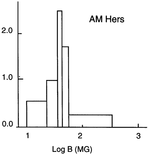
Fig. 39.— Normalized histogram of the field distribution of AM Hers in Table 2. Copyright Astrophysical Journal, reproduced with permission.
As the field is increased above 200 MG (e.g., as in the isolated MWDs Grw +70°8247, GD 229, or PG 1031+234; 200–1000 MG), the frequency of the cyclotron fundamental sweeps through the optical spectrum to the UV. At very high fields, the optical emission will be in the low‐frequency tail of the first harmonic in the optical and will be in the high‐field limit—that is, if the radiation is polarized, the polarization should be predominantly linear (see § 5.4.1). Given the high optical depth at the fundamental (which now occurs in the UV‐optical), the radiation emerging from these systems may be essentially unpolarized. However, at very high fields, the population of the Landau states is expected to be determined mainly by cyclotron cooling. In this case, the cyclotron fundamental may be formed by scattering (cf. neutron stars), and therefore some polarization may be expected.
Based on the experience with AR UMa, one can identify several selection effects which would work against the discovery of these higher field systems (Schmidt et al. 1996b). First, the electrons are cooled rapidly in the postshock region (the cyclotron cooling–dominated two‐fluid regime; see § 6.1.1), and the hard X‐ray temperatures typical of most AM Hers shocks are not achieved. These systems are therefore less likely to stand out in X‐ray surveys. Second, the strong magnetic field systems may be spending a high fraction of their time in a low state (a low duty cycle), following the general trend noted by Warner (1995). Thirdly, the very high field systems may not be strong emitters of circularly polarized radiation in the optical band.
We show in Figure 40 (bottom panel) the period distribution of AM Hers in Table 2. The data show a gradual increase in the number of systems with decrease in period with two spikes at 202 and 114 minutes, respectively. It is evident that the magnetic systems do not show as pronounced a period gap (lack of systems with periods between 2 and 3 hr) as do the nonmagnetic CVs (see Warner 1995 for an equivalent plot for all CVs), although the statistical significance of this result has been hotly debated in the literature (e.g., Beuermann & Burwitz 1995). From a physical point of view, there are strong reasons for expecting a different period distribution for the magnetic CVs. Orbital evolution longward of the period gap is driven mainly by magnetic braking due to the wind that emanates from the companion star. In the synchronized high‐field AM Hers, the wind tends to be trapped by the magnetosphere of the MWD, and under certain circumstances the magnetic braking can be reduced by several orders of magnitude (e.g., Li & Wickramasinghe 1998).
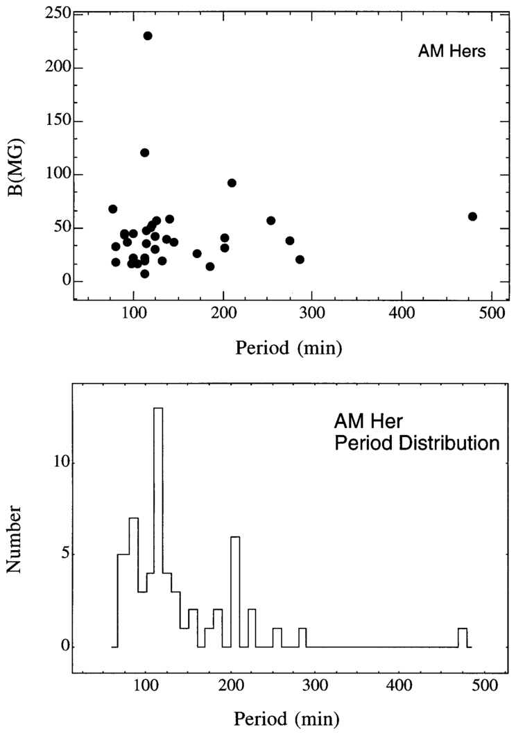
Fig. 40.— Top: The field‐period relationship for AM Hers in Table 2. Bottom: The period distribution of AM Hers.
Finally, we note that if mass transfer is conservative, one may expect the mass of the WD in a given system to increase as the orbital period decreases and that such a change may also be reflected in a change in the surface field strength, and therefore in the magnetic field distribution. An analysis of the magnetic field–period relation given in Figure 40 (top panel) shows that the magnetic field strength is strongly uncorrelated with the magnetic field. Furthermore, there is no evidence that the systems in the period gap (Porb = 120–180 minutes) have a field that is significantly different from that of the total sample.
6.3. Mass Determinations
Masses of the white dwarfs in the AM Herculis–type systems have been determined by measuring radial velocity variations of absorption lines from the photosphere of the companion star, of narrow emission lines attributed to the heated surface of the companion star, and from eclipse light curves of the white dwarf by the companion star. There are large uncertainties in interpreting the radial velocity curves of the narrow emission lines, since these may be distorted by contributions from the mass transfer stream. It may also be possible to use X‐ray emission lines (Cropper et al. 1998) or cyclotron lines (Visvanathan & Wickramasinghe 1979) to determine masses of the underlying white dwarf, but this may require careful modeling of the shocks at a higher level that is currently unattainable.
The radial velocity methods using lines from the companion star can be expected to give accurate results only for the brightest systems where high‐resolution observations have been possible of absorption lines (in particular, of the Na i lines λλ8183–8195). The errors in mass determinations using this method are dominated by uncertainties in the orbital inclination which is usually estimated independently from polarization studies. The most accurate velocity data are for AM Her itself by Young & Schneider (1979), who gave the mass of the white dwarf as M = 0.6 M⊙. Other similar studies have been reported by Mukai & Charles (1987), and the results are summarized in Table 2. V1500 Cyg, the only known magnetic nova, has the highest mass estimate (Horne & Schneider 1989), in line with the estimated mean mass for classical novae (Webbink 1990).
Only six AM Hers are eclipsing, and of these only two have so far been studied at sufficiently high time resolution to enable radii and masses to be determined. The eclipse method applied to UZ For (Bailey & Cropper 1991) and corrected for limb darkening yields a mass Mwd = 0.7 ± 0.09 M⊙. A similar study of DP Leo yielded Mwd = 0.71 M⊙ (Bailey et al. 1993). These values compare well with the mean mass of 0.74 found for CVs (Webbink 1990), although this sample also includes the more massive classical novae. If one considers all magnetic systems with mass estimates obtained using optical techniques (see Table 2), the mean mass is Mwd = 0.62 M⊙, but the errors in this estimate are probably quite large.
Based on a sample of 52 AM Hers, the space density of nearby short‐period AM Hers has been estimated by Beuermann & Burwitz (1995) to be 5 × 10⁻⁷ pc−3, thus about ∼10−2 smaller than that for isolated MWDs.
7. CONCLUSIONS
The isolated MWDs have fields in the range ∼0.1–1000 MG with a field distribution which peaks around of 16 MG. There is some indication that the distribution may fall off rather sharply below 0.1 MG. The data currently at hand supports the view that the magnetic fields of the isolated MWDs are of fossil origin with the parent stars being the magnetic Ap and Bp stars (B∼102–104 G).
Detailed studies of individual stars have shown evidence for complex field structures which can be modeled as a first approximation, by dipoles that are displaced by ∼10%–30% of the white dwarf radius from the center of the star. However, in some stars, there is clear evidence for even more extreme global field structures, which cannot be modeled by offset dipoles and indicate instead magnetic spot–type field enhancements. These stars occur among both high‐field and low‐field objects. The field strength appears to be uncorrelated with effective temperature, nor is there strong evidence for the evolution of field complexity along the cooling sequence. However, other parameters such as mass may be linked to complexity, but this remains to be investigated. The observations of the isolated MWDs do not in general support the free ohmic decay models for the field.
Various independent lines of evidence suggest that isolated MWDs have a mean mass (≳ 0.95 M⊙) that is significantly higher than that of nonmagnetic white dwarfs (0.57 ± 0.002 M⊙). The magnetic field may therefore play a dominant role in mass loss during post–main‐sequence evolution and influence the initial‐final mass relationship. There is also some evidence that the MWD mass distribution may be bimodal, with a second population having a mean mass closer to the Chandrasekhar's limit perhaps resulting from DD mergers. Here, there is the suggestion that the magnetic field, through its effect on the initial‐final mass relationship, may also have an influence on the outcomes of close binary evolution, including the birth rate of Type Ia supernovae.
The rotational velocities of the MWDs appear also to show a bimodal behavior. At one extreme there are the rapid rotators with rotation periods ranging from ∼700 s to several hours. These may have been the result of DD merger or spin up in a previous phase of close binary evolution. At the other extreme there is a group of stars which show no evidence for rotation with estimated rotation periods of ≳100 yr. Here the rotational velocities are expected to be larger than measured of nonmagnetic WDs, suggesting that the magnetic field may also spin down the core during post–main‐sequence evolution.
The MWDs in binaries appear to exhibit a level of complexity in field structure which parallels what is seen in the isolated MWDs. Thus the Zeeman and cyclotron spectra of the MWDs in some AM Hers require dipole offsets of up to 0.3%, while in others there is indirect evidence for quadrupolar field structures. The most accurate method for determining masses of the MWDs in the AM Herculis–type systems is through studies of the eclipse light curves and yields values consistent with the average mass estimated for the nonmagnetic CVs, namely, ∼0.7 M⊙.
Magnetic fields tend in general to be neglected in considerations of stellar evolution. However, the observed properties of the MWDs appear already to suggest that the magnetic field could play an important, if not dominant, role in determining the initial‐final mass relationship and also have an influence of the outcomes of binary stellar evolution. One of the major challenges which remain ahead would be the inclusion of magnetic fields, particularly in the post–main‐sequence phases of evolution. Another is the construction of realistic model atmospheres and line profiles for magnetic white dwarfs at arbitrary field strengths at a level of sophistication that will enable effective temperatures and gravities to be determined routinely from observations, as is currently done for nonmagnetic WDs. This latter goal can be achieved only through further theoretical studies on continuum and line opacities and of the effects of pressure broadening of line profiles in strong magnetic fields.
The authors would like to thank Dr. Stéphane Vennes for many discussions and Professor Gary Schmidt and Dr. Vennes for their careful reading of the manuscript and valuable comments. We are also grateful to Professor Peter Schmelcher for providing us with calculations of helium transitions at high magnetic fields in advance of publication.