
ABSTRACT
Results of the commissioning of the first Gemini Multi‐Object Spectrograph (GMOS) are described. GMOS and the Gemini–North telescope act as a complete system to exploit a large 8 m aperture with improved image quality. Key GMOS design features such as the on‐instrument wave‐front sensor (OIWFS) and active flexure compensation system maintain very high image quality and stability, allowing precision observations of many targets simultaneously while reducing the need for frequent recalibration and reacquisition of targets. In this paper, example observations in imaging, long‐slit, and multiobject spectroscopic modes are presented and verified by comparison with data from the literature. The expected high throughput of GMOS is confirmed from standard star observations; it peaks at about 60% when imaging in the r' and i' bands, and at 45%–50% in spectroscopic mode at 6300 Å. Deep GMOS photometry in the g', r', and i' filters is compared to data from the literature, and the uniformity of this photometry across the GMOS field is verified. The multiobject spectroscopic mode is demonstrated by observations of the galaxy cluster A383. Centering of objects in the multislit mask was achieved to an rms accuracy of 80 mas across the 5  5 field, and an optimized setup procedure (now in regular use) improves this to better than 50 mas. Stability during these observations was high, as expected: the average shift between object and slit positions was 5.3 mas hr−1, and the wavelength scale drifted by only 0.1 Å hr−1 (in a setup with spectral resolution of 6 Å). Finally, the current status of GMOS on Gemini–North is summarized, and future plans are outlined.
Export citation and abstract BibTeX RIS
1. INTRODUCTION
The Gemini Multi‐Object Spectrograph (GMOS) has become a workhorse optical instrument at Gemini–North since it entered regular science operation in late 2001. It has four main modes of operation: imaging, long‐slit spectroscopy, multiobject spectroscopy (MOS), and integral field unit (IFU) spectroscopy.
The GMOS‐Gemini–North (GMOS‐N) combination acts as a complete system to exploit a large 8 m aperture and improved image quality. This has been accomplished through carefully engineered design of the instrument structure and its many mechanisms. Indeed, the entire GMOS system (optics, mechanics, software, and detectors) was designed to take advantage of the best images that the Gemini telescope produces. During observations, the GMOS on‐instrument wave‐front sensor (OIWFS) maintains guiding and provides tip‐tilt, focus, and astigmatism signals, which are corrected in real time by the telescope primary and secondary mirror systems. As the telescope tracks, the image on the GMOS detector is held stable by an active flexure compensation system. As a result, GMOS on Gemini is routinely able to obtain sharp, stable images, allowing extremely deep observations of very faint targets. Furthermore, the OIWFS maintains the position of objects in multiobject slit masks over many hours (in part, by making use of a model to account for differential atmospheric refraction), thereby contributing to observing efficiency by reducing the number of time‐consuming checks of mask alignment on the sky.
After installation on the Gemini–North telescope in 2001 August, GMOS commissioning began with daytime work (characterization of flexure, etc.), followed by nighttime tests. In this paper, the main results are summarized from the nighttime commissioning of the imaging, long‐slit, and MOS modes. First results from the IFU commissioning have been presented by Allington‐Smith et al. (2002).
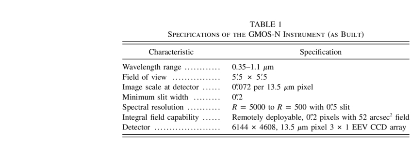
In a separate paper (Murowinski et al. 2004), details are presented of the instrument design and the extensive laboratory tests that the instrument underwent before shipping. Comprehensive overviews of the GMOS designs, including novel features such as the OIWFS and flexure compensation system, have been presented elsewhere (Davies et al. 1996; Murowinski et al 1998, 2004; Crampton et al. 2000). A summary of the main instrument specifications is given in Table 1, and a schematic diagram of the detector array is shown in Figure 1.

Fig. 1.— Schematic diagram showing the layout of the three GMOS detectors that form the 6144 × 4608 pixel array. There are small gaps between the detectors of about 0.5 mm, corresponding to about 37 pixels. The imaging field of view occupies the central region of the array and is shown by the shaded region. The on‐instrument wave‐front sensor patrol field, projected onto the detector plane, is shown by the dotted line. Note that there is a reflection in the vertical direction between the detector plane shown here and the mask plane shown in Fig. 3 of Murowinski et al. (2004). In spectroscopic mode, a slit mask is moved into the beam to cover the imaging field, and the resulting spectra run horizontally across the CCD array. In the long‐slit case, the slit runs vertically up the center of the field.
 |
In the following sections we describe nighttime observations that were used to test the on‐sky performance of GMOS in imaging, long‐slit, and multiobject spectroscopic modes.
2. THROUGHPUT MEASUREMENTS
GMOS was designed to be a high‐throughput spectrograph and makes use of special optical coatings and glasses (including large calcium fluoride lenses) to meet this goal in addition to tight specifications on image quality (Stilburn 2000; Murowinski et al. 2003b). Laboratory measurements of the throughput of individual components that make up GMOS, including the EEV CCDs, are shown in Figure 2. In this section, the expected response of GMOS based on these response curves is compared to the throughput measured from observations of standard stars.
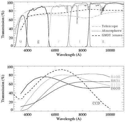
Fig. 2.— Response functions, measured in the laboratory, for various elements currently in use in GMOS‐N. The upper panel shows the transmission of the four original science filters, g',r',i' and z', plus the new u' filter, which form a set similar to the SDSS set (Fukugita et al. 1996). The throughput of the main optics (i.e., the collimator and camera lens groups) is shown by the dashed line. Also plotted are the telescope and atmospheric response functions assumed in the GMOS throughput calculation (see text). The lower panel shows the average quantum efficiency curve, measured with the detectors cold, for the three EEV (now E2V) CCD chips (dashed line). Also plotted are the response functions of the gratings, R150, R400, B600, and R831 (solid lines). The grating responses were measured in Littrow configuration by the manufacturers, but have been corrected in this figure to account for the non‐Littrow configuration in GMOS. Note that this is an approximation and that anomalies in the efficiency (sharp peaks and troughs) are difficult to predict when the geometry changes.
2.1. Throughput in Imaging Mode
The throughput of the GMOS‐Gemini–North system in imaging mode was measured from observations of the standard star field PG 1323‐086 (Landolt 1992), observed on 2003 February 5. GMOS was mounted on one of the side‐looking ports of Gemini–North during these observations. The data were reduced with the Gemini IRAF package,2 using dome flat fields taken during the commissioning run.
Table 2, column (4) gives the predicted absolute throughput of GMOS based on the transmission of the main optics, i.e., the collimator and camera lens groups, the filters, and the mean quantum efficiency of the CCDs (see Fig. 2) at the central wavelengths of the imaging filters. These response functions were multiplied together with the telescope and atmosphere response functions, also given in Table 2, and were used to derive expected counts for a given standard star magnitude (assuming spectral types, which were chosen based on the published broadband colors from Landolt [1992]). The telescope response function used in this calculation was derived from the theoretical reflectivity of aluminium for the Gemini–North primary and secondary mirrors, and that of silver for the tertiary ("science fold") mirror. The primary and secondary reflectivity functions were scaled by a factor 0.96 to best match real reflectometer measurements made at 470, 530, 650, and 880 nm. The tertiary mirror reflectivity was scaled by a factor 0.91 to coincide with a single reflectometer measurement at 670 nm. All reflectometer measurements were made within 1 month of the observations reported here. The overall telescope reflectivity function derived in this way is shown in Figure 2. Note that the telescope response function assumed in the Gemini‐GMOS Integration Time Calculator (ITC), available on the Gemini Web pages, does not include the scaling factors used here. The preliminary throughput values reported in Hook et al. (2003) also omit these factors and were relevant for data taken on the up‐looking port, which involves one fewer reflection.
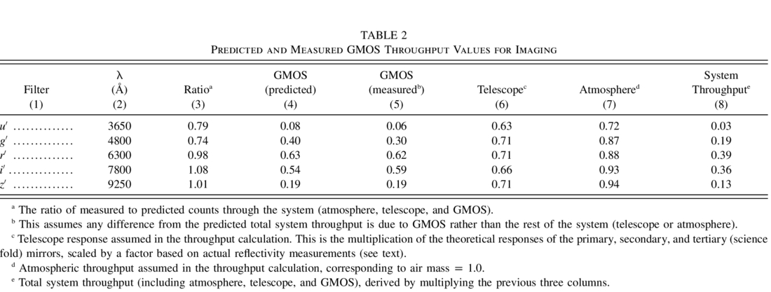 |
The ratio of measured to expected counts through the system (atmosphere, telescope, and GMOS) is given in Table 2, column (3). The throughput in the redder filters (r', i', and z') is very close to expectation, but is somewhat lower than expected in the bluer filters (u' and g'). This deficit of ∼20% in the blue is not understood and is still being investigated. It should also be noted that the median extinction of Mauna Kea was assumed, and no independent measurements of the extinction were made on the night of observation.
In order to derive an estimate of the absolute GMOS instrument throughput, the difference between expected and measured counts is assumed to be entirely within GMOS; i.e., the rest of the system (telescope, atmosphere) is assumed to behave exactly as predicted. The resulting derived GMOS instrument throughput values, which include the effect of all the GMOS optical components and the EEV CCDs, are shown in Table 2 and Figure 3. As can be seen, the response of GMOS in imaging mode is high, peaking at ∼60% in the r' and i' bands.

Fig. 3.— (a) Ratio of measured to expected counts through the Gemini‐GMOS system, including the telescope and atmosphere, in spectroscopic mode (solid curve) and imaging mode (squares). The measured counts are from standard star observations taken on 2003 February 5. The expected counts were predicted using the GMOS throughput curves shown in Fig. 2, the measured reflectivity of the Gemini mirrors on dates close to the observations, and atmospheric extinction corresponding to the air mass of the observations. (b) Absolute throughput of the GMOS instrument expected in spectroscopic mode (dashed line) and imaging mode, calculated at the central wavelength of the imaging filters (open squares). This includes all the optical components of GMOS and the EEV CCDs, but does not include the response of the telescope and atmosphere. The measured throughputs (solid line and filled squares) are derived from the standard star observations above, assuming that any difference from the expected total system throughput is within GMOS, and not due to incorrect assumptions for the throughput of the telescope or atmosphere.
Finally, the total system throughput in imaging mode (including atmosphere, telescope, and GMOS) is given in the right‐hand column of Table 2.
2.2. Throughput in Spectroscopic Mode
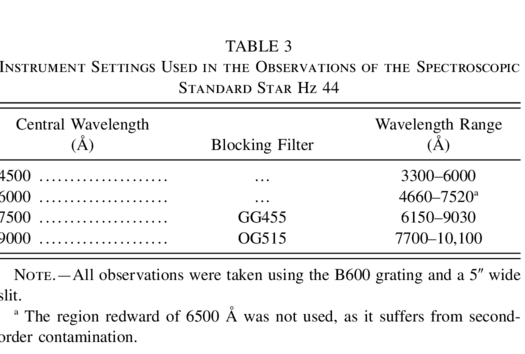
The spectroscopic standard star Hz 44 (Oke 1990; Massey et al. 1988) was observed through a 5'' wide slit on the night of 2003 February 5, the same night as the imaging observations described above. The observations were taken with the B600 grating at four central wavelength settings to cover the full useful wavelength range of GMOS. These settings and the order‐sorting blocking filters used are listed in Table 3. In the comparison below, any regions of the spectra that could be contaminated by second‐order light were not used.
 |
Predicted counts through the GMOS‐Gemini–North system were calculated by multiplying the relevant response functions of the atmosphere, telescope, and GMOS components. The input spectrum was that of Hz 44 normalized in the V passband using the broadband magnitudes given in Massey et al. (1988). A correction was made to the predictions to allow for the non‐Littrow configuration of the B600 grating in GMOS, estimated using the PCGrate software (see Murowinski et al. 2004 for details). The resulting response function is shown in Figure 2, along with those of the other optical components in GMOS.
The ratio of the measured to predicted counts (in electrons) was then calculated as a function of wavelength for each spectrum. A smooth sixth‐order polynomial was fitted through the ratio spectra, and this curve is plotted in Figure 3 a.
The measured throughput of GMOS alone is plotted in Figure 3b (solid line). As for the imaging case, this has been derived assuming that the difference between predicted and measured counts is entirely due to GMOS.
By comparison with the imaging throughput measurements taken on the same night (squares in Fig. 3a), it can be seen that the spectroscopic throughput is somewhat lower than expected at very red wavelengths (>8000 Å), even allowing for the presence of the grating. This difference is also not understood, but suggests that the throughput of the B600 grating is not well predicted, perhaps because of the non‐Littrow configuration of GMOS (see Murowinski et al. 2004 for details of the method used and the difficulties associated with these grating response predictions).
Although somewhat lower than predicted, the throughput of GMOS is still very high in spectroscopic mode, peaking at about 45% at 6300 Å with the B600 grating in place. However, the B600 is not the most sensitive of the GMOS gratings at this wavelength. Assuming the relative response functions in Figure 2, the R150 grating would give a peak GMOS response of more than 50% in spectroscopic mode at 6300 Å.
A direct comparison of the efficiency of GMOS with other imaging spectrographs on 8–10 m telescopes is not straightforward, because results are reported in a variety of different ways and are based on different assumptions. The spectroscopic throughput (not including telescope or atmospheric extinction) of the original Keck LRIS spectrograph (Oke et al. 1995) peaked at ∼30%, but with more modern, more efficient detectors, this has increased to ∼40% (as described by J. Cohen on the Keck/LRIS Web pages). Kashikawa et al. (2002) report that the total (including telescope) throughput of FOCAS on the Subaru 8 m peaks at ∼32%, and Sheinis et al. (2002) report even better results of ∼42% peak system efficiency (after removing the effects of the atmosphere but including the telescope) for the Keck ESI spectrograph in low‐resolution mode. GMOS therefore lies towards the upper end of 8 m class spectrograph efficiencies.
3. VERIFICATION OF IMAGING MODE
In the following sections, we demonstrate the use of GMOS for scientific observations in imaging, long‐slit, and MOS modes. The simplest mode is imaging, in which the GMOS fold mirror (rather than a grating) is moved into the beam, and there is no slit mask in place. The acquisition process involves slewing the telescope to the field and starting guiding with the OIWFS on a bright star.
The primary requirement on the GMOS imaging mode was that it could be used to provide images for MOS mask design. In practice the GMOS imaging mode is also used for deep imaging, photometry, and morphology studies. Examples of deep‐imaging observations include the "system verification" observations of the field of the quasar PMN 2314+0201 (with data available via the Gemini Web pages) and observations of the William Herschel Deep Field, described below.
3.1. Imaging of the WHDF
The William Herschel Deep Field (WHDF) has been the subject of extensive optical CCD photometry taken on the 2.5 m Isaac Newton Telescope and 4.2 m William Herschel Telescope (WHT) at the Observatorio del Roque de los Muchachos on La Palma (Metcalfe et al. 1995, 2001). A region of this field was imaged with GMOS during commissioning in order to design a mask for MOS follow‐up. Below we describe the imaging data (which will be made public) and compare it with the existing photometry.
3.1.1. Data Obtained
The GMOS imaging data were taken on the night of 2001 August 20 (UT). Six exposures of 300 s were taken in each filter (g',r',i',z') in seeing conditions ranging from 0  56 to 0 72 FWHM in individual exposures. The images in each filter were bias subtracted, flat‐fielded and combined using the Gemini IRAF data reduction scripts.
These data overlap WHT B, R, and I data, which reach 3 σ detection limits of B∼27.9, R∼26.3, and I∼25.6 (Metcalfe et al. 2001). The seeing on these images ranges from 1 25 to 1 5, and is thus substantially worse than that on the GMOS frames.
3.1.2. Data Analysis
In order to compare the WHT data with that obtained with GMOS, the combined GMOS frames were reduced in identical fashion to the original WHT data. This technique is described in detail in Metcalfe et al. (1995), but a brief summary is given here.
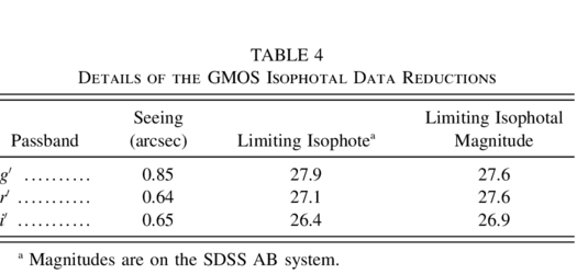
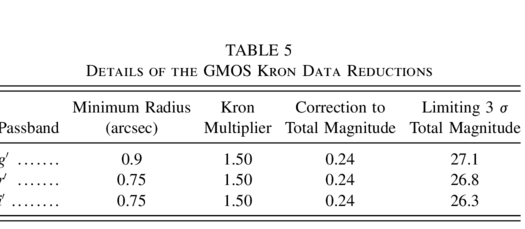
First, after a polynomial fit to the background sky had been removed, an isophotal detection scheme was run over the GMOS image as faint as is practical given the noise level on the sky. All images detected this way were then deleted from the image and replaced by random noise. The resulting image was then heavily smoothed using several passes of a box filter a few arcseconds in diameter, and the result was subtracted from the original image. This produces an extremely flat sky background, which is necessary because the image detection technique used here does not calculate a local sky level. The isosphotal detection scheme was then rerun, and the resulting object locations passed to a Kron magnitude measuring program, which produces the final magnitudes for the objects. A minimum Kron radius equivalent to that for stellar images was set, and a small multiplying factor was used in order to reduce the amount of deblending required. Thus, the corrections to total magnitudes are quite large. Parameters for the data reduction can be found in Tables 4 and 5.
 |
 |
3.1.3. Zero Points and Color Equations
To zero point the GMOS photometry, observations of the standard star field PG 0231+051 were used. These were taken at the same air mass as the data frames, so no atmospheric extinction corrections were needed. As the GMOS filter, optics, and CCD response functions (Fig. 2) give a system very similar to that of the Sloan Digital Sky Survey (SDSS), the frames were calibrated on the SDSS AB system using the SDSS magnitudes for the Landolt (1992) standards, which are distributed in a calibration file within the Gemini IRAF package.
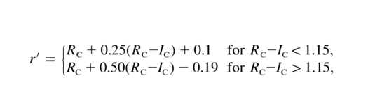
To compare with the WHT data (which is close to the standard Johnson‐Cousins photoelectric system; Metcalfe et al. 2001), the following observational transforms between the standard photoelectric passbands and the SDSS system given in Smith et al. (2002) were applied to the WHT magnitudes:


The i‐band was more problematic, as there is no direct transform in Smith et al. (2002). However, by combining their (RC−IC) transform with the rSDSS−RC relation above, the following transformations were deduced:


and
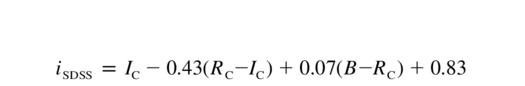

When comparing WHT and GMOS magnitudes in our data, it became obvious that the transform for the redder objects is not valid (it gave a far worse fit than simply applying the bluer transform to all objects). From our data it is not possible to distinguish whether this is caused by a difference in the GMOS and SDSS instrumental systems, or by a problem with the Smith et al. (2002) rSDSS−RC versus B−RC relation for very red objects. Inspection of our data reveals that although this relation is valid for (B−RC)<2.2, for colors redder than this the slope increases sharply to ∼ 0.6(B−RC). Fitting (by eye) to the brighter stars in our data, the following empirical relations are found for 0<(RC−IC)<2:
and

where m' denotes the GMOS magnitude in filter m on the SDSS magnitude system, and (RC,IC) here denote WHT magnitudes in the Johnson‐Cousins system. The slopes are only accurate to ∼0.025, but the amount of data available for comparison is limited. The offset terms also depend on the relative accuracy of the two sets of zero points, which is probably no better than 0.05 mag. Note that there is no change of slope in the i‐band transform at (RC−IC) = 1.15, but rather a linear transformation is valid out to the red limit of the data.
3.1.4. Magnitude Comparison
Magnitudes from the WHT and GMOS data were compared both as a function of magnitude and of radial position from the center of the GMOS image. It should be noted that with such deep images, deblending of merged objects is frequent and seeing‐dependent. The very different seeing between the two data sets means that this procedure can introduce noise into the comparison, even at bright magnitudes. As a result, our comparison was restricted to objects that have not been flagged as deblended on the GMOS image. The results are shown in Figures 4 and 5. For g'<23, r'<23, and i'<22, the following comparisons were found:


where the WHT magnitudes have been converted into the SDSS system using the relations in Smith et al. (2002), as described in § 3.1.3. No significant difference between the three GMOS CCD chips was found. In addition, no discernible radial gradient was found in the comparisons for any band, consistent with a ray‐tracing analysis that shows that GMOS does not vignette the 7' diameter field delivered by the Gemini science fold mirror. Although the offsets (all in the sense that the GMOS magnitudes are fainter than the WHT) are larger than might have been hoped, especially in the i'‐band, these are perhaps not surprising, given the difficulties in transforming to the SDSS system.

Fig. 4.— Comparison between GMOS and WHT magnitudes (after color correction) for g'‐band, r'‐band, and i'‐band. The different symbols indicate on which of the three original individual chips the objects lie. Only isolated objects are included.

Fig. 5.— Comparison between GMOS and WHT magnitude (after color correction) as a function of radial distance from the center of the GMOS field of view, again for g'‐band, r'‐band, and i'‐band. Only the brighter objects are included in these plots.
3.2. Ghost Images and Scattered Light
Considerable attention was paid in the optical design of GMOS to ensure that parasitic and scattered light was kept to a minimum. The CCD detector surface is relatively reflective (at some wavelengths more than others), and light returning from the detector can be scattered back again from one or more of the optical surfaces.
Careful optical design, baffles, and very efficient antireflection coatings on the GMOS optics help reduce such effects. However, small ghost images are apparent in part of the field, with surface brightness approximately 0.3% that of the parent images. These ghosts are approximately in focus, and their integrated flux is also approximately 0.3% that of the corresponding parent image. The ghosts are believed to be reflections off the filters, and rotate around the field as expected when the filter cells are rotated. The filters were originally designed with a 3° tilt in an attempt to avoid this problem, but subsequent ray tracing shows that a tilt of almost 6° is necessary to completely eliminate them from the entire field. The manufacture of new holders that will increase the tilt of the filters is being planned.
A second type of ghost image has been seen in a small number of GMOS frames. These ghosts are large, circular, fairly sharp edged patches of light approximately 4 3 in diameter. An artifact of this type was seen in the deep imaging of the field around the quasar PMN 2314+0201, which was observed as part of system verification. The light patch had surface brightness approximately 0.9% above the background in the g'‐band, and approximately 0.1% above the background in the i'‐band (it was not seen in the r'‐band images). On one occasion during GMOS queue observations, a similar but much brighter artifact was seen, with a surface brightness approximately 23% above the background. It is believed that these artifacts are related to bright stars near the fields—in the case of PMN 2314+0201, there is a 7.6 mag star 0  3 from the target, and in the second case there is a 1.6 mag star 0 5 from the target. The route this light is taking to the GMOS detectors is not known.
3.2.1. Parasitic Light
A common problem with focal reducing optics is that light scattered back from the relatively reflective CCD surface can be reflected back to the detector, producing an enhanced background. Furthermore, this "parasitic light" is frequently concentrated into a diffuse spot at the center of the field, which may be 5%–10% above the background. The GMOS optics were designed to minimize this problem; nevertheless, our tests indicate that there is some undesirable parasitic light at bluer wavelengths. Sky flats in i' and z' exhibit variations with an amplitude of a few percent that appear, from their structure, to be a result of the thinning processes of the CCD detectors. However, the variations in g' reach an amplitude of up to 7% from center to edge of the field, and hence may be partly due to parasitic light. This possibility is partly supported by systematics observed in calibrated photometry of about 0.03–0.05 mag, which appear to be worst in the g'‐filter, although the limited data useful for these tests are not completely conclusive on this aspect. Since the antireflection coatings of the detectors for GMOS‐N are red optimized, light reflecting from the detector surface would be brighter in the blue and could be partially responsible. Thus, additional care must be taken to produce precision photometry, especially at wavelengths blueward of 7000 Å.
3.3. Fringing in Imaging Mode
The EEV CCDs in GMOS–North have significant fringing in the red. In imaging mode the fringe strength in the z'‐filter is typically ±2.5% of the background, while in the i'‐filter the fringing is ±0.7% of the background.
The fringing in imaging mode can be removed effectively by subtraction of a fringe frame for the relevant filter. This frame is typically constructed using several images of the sky taken in conditions similar to those in which the science data were obtained. In cases in which the science data consist of many dithered images, these frames themselves can be used to construct a fringe frame. This is done by masking objects and combining the flat‐fielded frames (without shifting). In the case of i'‐band data, the fringe frame is median smoothed with a box size of 31 × 31 unbinned pixels to increase the signal‐to‐noise ratio. However, z'‐band fringe images cannot be smoothed, because there are fringes on a spatial scale of a few pixels. The fringe frame is then subtracted from each science frame. Example fringe frames in i' and z' imaging mode obtained during commissioning can be found on the Gemini Web site.
4. VERIFICATION OF LONG‐SLIT MODE
Although GMOS is a very effective imaging instrument, its primary function is as a spectrograph. In the following sections we give examples of GMOS used in spectroscopic mode, starting with the simpler case of long‐slit observations of a single object, and followed in § 5 by an example of multiobject spectroscopic observations.
The long‐slit masks in GMOS can be thought of as special cases of MOS masks. They were cut from the same type of material using the same laser cutter, and they are loaded into the instrument in the same way. The long slit masks each have two small bridges to hold the two halves of the mask in place. These bridges are 2 mm (3 2) long and divide the long slit into three equal segments. It is planned to fabricate new long‐slit masks out of thicker material so that the bridges will not be necessary.
Targets for long‐slit spectroscopy are typically aligned with the slit, using the following procedure. After slewing to the field and setting the Cassegrain rotator angle to the desired position angle on the sky, an image is taken of the field, and the position of the target is measured from the image. This position is then compared to the position of an image of the long slit (taken earlier), and the telescope offsets needed to bring the target to the center of the slit are calculated using the known pixel scale at the GMOS detector. This image can also be used to adjust the position angle if necessary (for example, to align two objects along the slit). The offsets (and position angle adjustment) are applied, and the long‐slit mask is moved into the beam. An image through the slit is then taken to check the centering, and small offsets are applied if necessary to accurately center the target(s) in the slit.
In cases in which the object is too faint to be easily visible in an acquisition image, the above procedure can be carried out on a nearby bright star with known offsets to the target. Once the offset star is well centered, the telescope is offset to the target, and no further acquisition images are taken. Once the target is aligned with the slit by one of these methods, the GMOS mirror is then exchanged for a grating, and spectroscopic observations begin. The accuracy of offsetting has been shown to be better than 0 1 over a 20'' offset. However, it is possible that the accuracy of offsetting may depend on the position of the OIWFS probe within its patrol field. Since a full mapping of the offset accuracy has yet to be carried out, the direct imaging method is the recommended method for long‐slit target acquisition. Principal investigators should consult with Gemini staff if they wish to use the offsetting method in a queue program.
4.1. Long‐Slit Spectroscopic Observations of PMN 2314+0201
The z = 4.11 quasar PMN 2314+0201 was observed on the night of 2001 August 15 (UT) as a test case for long‐slit spectroscopic observations and data reduction. This object is relatively bright (r' = 20.0; Hook et al. 2002) and was aligned with the slit using a 30 s r'‐band acquisition image followed by a 60 s through‐slit image.
The spectroscopic observations consist of a 900 s exposure with the B600 grating at a central wavelength setting of 6000 Å, giving a wavelength coverage of 4430–7290 Å. A 1 0 slit was used, with a resulting spectral resolution of 6 Å. The observations were taken when the target was at air mass = 1.08, and the seeing was 0 6 FWHM (estimated from a cut through the QSO spectrum in the spatial direction). Matching flats and arc comparison spectra were taken immediately after the quasar observation. Observations of the spectrophotometric standard Hiltner 102 were also obtained with the same grating setting but with a 5 0 slit, in order to flux‐calibrate the quasar spectrum. All the spectroscopic data were taken with the CCD array windowed in the spatial direction (CCD‐y) to the central 1000 pixels.
The data were reduced using the spectroscopic tasks of the Gemini IRAF package. The data were first bias‐subtracted and flat‐fielded. In order obtain accurate sky subtraction, the two‐dimensional quasar spectrum was then corrected for small distortions that cause spectral lines to appear slightly curved rather than perfectly straight along the CCD columns. The size of distortion depends on the grating used—in this case the lines at the extreme red end of the spectrum were bowed by about 2 pixels (0.9 Å) from the central row of the readout window to the upper and lower edges. The distortion across the two‐dimensional spectrum was mapped out using the task gswavelength. In this case a fourth‐order Chebyshev function was used to fit the transformation in both CCD‐x and CCD‐y.
The derived transformation was then applied to the two‐dimensional quasar spectrum. The sky lines in the two‐dimensional transformed quasar spectrum were then used to check the accuracy of the transformation. The sky lines were found to be straight to within ∼0.5 pixels (0.2 Å), and the wavelength calibration was found to be accurate to 0.16 Å rms. These residual errors are within the measurement uncertainty for these lines, since the 1'' slit has a projected width of 13.8 pixels (6.2 Å).
Following wavelength calibration and sky subtraction, the one‐dimensional spectrum was extracted and flux calibrated using the standard star spectrum, which had been reduced in the same way as the quasar spectrum.
Figure 6 shows the GMOS data compared to observations of the same object from the literature (Hook et al. 2002), taken with the Faint Object Spectrograph and Camera (ver. 2, EFOSC2) at the ESO 3.6 m in 1998 October. This is a 600 s spectrum taken using the EFOSC2 R300 Grism (No. 5) and a 1 5 slit, giving a spectral resolution of ∼19 Å. The object was at air mass 1.05 during these observations, and seeing was 1 2 (measured from the acquisition image). Despite the fact that neither this nor the GMOS spectrum was intended to be a spectrophotometric observation, their absolute flux levels agree extremely well and are within the 1 σ statistical errors over most of the overlapping spectral range (see Fig. 6). This agreement is perhaps somewhat fortuitous, since the slit losses in the two quasar spectra would not be exactly the same. When the respective seeing and slit widths are considered, approximately 83% of the quasar flux would have fallen down the slit in the GMOS observations, and approximately 76% in the EFOSC2 spectrum. Thus, we may have expected a systematic difference of about 8% in absolute flux between the two spectra. In fact, this might explain the small systematic difference at the red end (where additional slit losses from atmospheric refraction are negligible).

Fig. 6.— (a) Example of a fully reduced GMOS long‐slit spectrum, a 900 s exposure of the z = 4.1 QSO PMN 2314+0201. (b) Comparison of the GMOS spectrum (dashed line) with a spectrum of the same object taken at the ESO 3.6 m (solid line; Hook et al. 2002). The GMOS spectrum has been smoothed to match the resolution of the ESO spectrum. (c) Difference between the two spectra (ESO spectrum subtracted from the GMOS spectrum, solid line) compared to the ±1 σ uncertainty (dashed line). Note the expanded flux scale. The slightly increased errors around the Lyα line at 6200 Å are probably caused by an imperfect match of resolution.
4.2. Fringe Correction in Spectroscopic Mode
In spectroscopic mode the effective spectral bandpass for each pixel is narrower than for imaging mode, and the fringing amplitude is therefore larger, typically ±12% at 9000 Å. Fringes can be removed effectively during spectroscopic data reduction by dividing the science frame by a flat‐field frame taken with the same instrument settings. However, because the amplitude of the fringes is large, even a small movement of the fringe pattern (introduced, for example, by flexure within GMOS) will cause the flat‐fielding accuracy to degrade. GMOS flexure tests show that with the active flexure compensation system running, residual uncorrected flexure is approximately 3 μm rms at the detector in the spectral direction, or 0.2 pixels rms, for random pointings of the telescope. This corresponds to the case in which daytime calibration is used to flat‐field nighttime science observations. Although this residual flexure is only a fraction of a pixel, the corresponding flat‐fielding error is around 1% (peak‐to‐valley residual at 8000 Å), which is a significant error for some scientific applications.
Therefore, when observing at the red end of the spectrum during normal science operations, it is recommended to take flat‐field spectra (illuminated by the facility calibration unit, GCAL) approximately every 1–2 hr, interspersed with the science spectra. Tests show that flat fields taken every hour reduce the flat‐fielding error to about 0.2% (peak‐to‐valley residual fringing) at 9500 Å.
5. VERIFICATION OF MOS MODE
Multislit masks with GMOS can be used to obtain spectra of many objects simultaneously. These masks are typically designed based on images taken with GMOS itself, and the coordinate transformations used to convert image coordinates into slit positions on a mask are described below. The MOS acquisition process and the accuracy to which objects can be centered in the slits is then described, using example data from the field of the galaxy cluster A383.
5.1. Coordinate Definition and Transformations
There are two coordinate transformations that most interest the users of GMOS data: those that map the sky to the image data file, and those that map the mask‐making design coordinates to the image data file. Other instrument frames of reference, such as that of the physical mask plane near the telescope focus, can be thought of as intermediate points that although necessary for instrument engineering or operation, can be largely ignored by users of the data.
5.1.1. Sky to Image File Transformation
The sky positions are recorded on the multiextension FITS data files through the use of a world coordinate system (WCS) in the raw data file. There are WCS entries for each of the three CCDs in the focal plane, defining the WCS for that CCD with respect to a single reference pixel for the array (the GMOS pointing origin) located at about the middle of the central chip, CCD2. The WCS entries are generated from two components: information on the telescope pointing that is gathered from the telescope control system at the time of the observation, and a fixed calibration that was determined during the GMOS commissioning period. The fixed calibration establishes the geometric position of each of the three CCDs with respect to the GMOS pointing origin, and is measured by noting the position (in pixels on the array) of a bright star for various offsets of the telescope pointing, typically six pointings distributed over each CCD. The relative accuracy of the WCS over the GMOS field is better than 0 1, but the absolute accuracy on the sky is less good and still under development, giving occasional errors at the time of writing that are of the order of 10''. The cause of this error is not yet known, although a simple pointing error can be ruled out. In most cases the absolute accuracy is better than 5''.
During data reduction, data from the three CCDs are typically mosaiced onto a single image extension using the Gemini IRAF task gmosaic. This is done to take into account the small misalignments (shifts and rotations) between the three CCDs in the array. Relative to the central chip (CCD2), CCD1 is shifted by 1.5 pixels in the CCD‐y direction and is rotated by 0 004, whereas CCD3 is shifted by 1.0 pixels in CCD‐y and rotated by 0 05. The gmosaic task regrids the outer two CCDs onto the WCS used by the central chip, leaving only one valid WCS entry in place for the whole field. In addition, gmosaic takes advantage of internal knowledge of chip‐to‐chip displacements that is more accurate than what is provided in the imaging WCS to achieve a continuity of image position at interchip boundaries to the level of about 15 mas (1/5 pixel). Files created after extraction of spectra will have a WCS that includes the wavelength scale in the pixel extension used for each slit, and also contain the original image WCS in the primary header unit.
5.1.2. Mask Design Coordinates to Image File Transformation
Objects that are to have slitlets cut and be measured spectrally have their coordinates measured from GMOS images. The actual position of the slit may differ from that designed, because of distortions in the mask fabrication process, and the image of that slit on the GMOS detector will be further distorted by instrument optics. The challenge is to know what mask design coordinates will result in a slitlet that is located at the same place in the input focal plane as that occupied by the celestial object.
GMOS currently takes advantage of the simplification that if GMOS images are used as the source of position information, then it is not necessary to know the precise position of objects on the mask frame of reference; it is only necessary to measure the total distortion between the mask design and the image file to make masks that place slits accurately in the mask plane. A future objective is to be able to make masks directly from sky coordinates gathered with any other instrument of sufficient accuracy, but to date, that capability has not been developed or tested. However, if deep imaging from another facility exists, one option is to translate the target coordinates into GMOS image coordinates, using bright reference stars observed in a short GMOS exposure of the field.
The transformation from mask design coordinates to image file coordinates is measured with the use of a special focal plane mask containing a rectangular grid of pinholes. The mask was designed with an array of 21 × 21 pinholes, each 10.00 mm (16 1) apart, covering the GMOS imaging plane. The mask was then fabricated using exactly the same software, tools, and techniques used for GMOS slit masks, hence incorporating any repeatable misalignment and distortion in that process. The mask was installed in GMOS and imaged in r'‐band at operating temperature, and the resulting data were mosaiced with the standard GMOS tasks to arrive at the measured position of the pinholes in a GMOS image. The IRAF task geomap was used to determine the fifth‐order polynomial, including cross terms, mapping the image file positions to mask design positions. That correction is routinely applied by Gemini during the mask fabrication process to the slit positions that the user has determined from GMOS imaging data.
5.2. Example MOS Data: A383
The galaxy cluster A383 (Abell 383, z = 0.187) was observed on the nights of 2001 August 21, 26, and 27 (UT) as a test of the MOS observing process including preimaging, mask design, MOS field acquisition, spectroscopic observing, and data reduction. Figure 7 shows the preimaging observations, which were made up of six observations of 300 s in the r'‐band, dithered by 5'' steps to cover the gaps between the chips. Matching g'‐band data were also obtained. The image quality in the r'‐band data was approximately 0 65 FWHM.

Fig. 7.— Top panel: Full‐frame (55 × 55) GMOS image of the cluster A383 taken in the r'‐band. The shadow of the on‐instrument wave‐front sensor probe is visible in the lower right quadrant. The gaps between the detectors have been covered by combining several dithered images. The area of the detector array that is not illuminated in imaging mode has been masked out during the data reduction process. The positions of the four acquisition objects are marked with boxes, and the 20 science targets are marked with circles (the diameter of the circles is approximately equal to the slit lengths). The spectrum of the object marked with a double circle is shown in Fig. 9. Bottom panel: Corresponding raw MOS data. Longer wavelengths are to the left. The gaps between the three CCD detectors are visible as vertical strips.
From these data a mask was designed with 1 0 wide, 9'' long slitlets placed on 20 objects in the field. In this case only one bank of slitlets was used, since the full width of the detector array is required for spectral coverage when using the B600 grating. Note that when a lower resolution grating is used, slits can be arranged in banks so that many more objects can, in principle, be arranged on one mask, typically 70–80 if using two banks. In addition, four 20 × 20 boxes were included in the mask design for bright acquisition objects. The acquisition objects are used to align the mask to the sky as described below.
5.3. MOS Acquisition Accuracy
The usual procedure for GMOS mask alignment on the sky is to center a small number of relatively bright acquisition objects in their corresponding 2'' × 2'' square holes in the mask. This is done by imaging these objects through the mask and applying small offsets to the telescope pointing and rotator angle. Once the acquisition objects are well centered, the GMOS grating is moved into the beam, and spectroscopic observations begin.
The setup on the A383 field was done "manually" by calculating shifts and rotations based on two or three of the acquisition stars (the procedure has since been automated and uses all the available acquisition stars in any mask, as described below). Since most of the objects targeted in the A383 mask are relatively bright galaxies, they are clearly visible through the slits in the acquisition images and can be used after the fact to determine the accuracy of the mask alignment procedure. The through‐slit acquisition image taken immediately before the MOS observations has since been analyzed for this purpose. This is a 60 s image taken through the r'‐filter in a seeing of 0 52 FWHM. From this, object centers for 15 of the brightest objects were measured using the IRAF task imexamine. The positions of the slit centers were measured by taking the average position of the slit corners, and the uncertainty on this measurement was estimated to be 0.09 pixels.
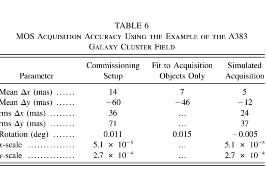
Figures 8a and 8b show the results of the analysis. In summary, the galaxies were reasonably well centered (rms error = 36 mas in CCD‐x, 71 mas in CCD‐y). However, the offsets appear to be systematic, in particular there appears to be a small rotation and scale error. This scale error is measured to be 2.68 × 10⁻⁴, which contributes an error of ∼1.2 pixels (∼90 mas) in the CCD‐y direction from one edge of the field to the other. The rotation error is small (0 011) but still corresponds to an error of 0.9 pixels (60 mas) across the field.

Fig. 8.— (a) Positional errors between the object centers and slit centers for all objects in the A383 mask, measured from an acquisition image immediately before the start of MOS spectroscopic observations. Acquisition objects are shown as filled circles, target galaxies are shown as open circles. (b) Positional error vectors magnified ×500 as a function of position in the field. Panels (c) and (d) show the same analysis on a second through‐slit image taken approximately 2 hr later, with no offsets having been applied in the meantime. The object positions have remained stable relative to the slit positions to better than 10 mas averaged over the field. Panels (e) and (f) show the centering accuracy that would have been achieved using the MOS acquisition alignment procedure that is now used in regular science operations.
Later in the commissioning process, an automated IRAF script was written to calculate the telescope offsets and rotation needed to align all the acquisition objects in real time. Figures 8e and 8f shows the results that would have been obtained had we used this procedure on the same acquisition image described above. To do this simulation, the alignment algorithm was run on the four acquisition objects to derive the telescope shifts and rotation that should have been applied to optimally align these objects. The measured coordinates of all the objects were then transformed by this amount to simulate telescope offsets. The resulting positional errors of the objects relative to their slit positions are shown in Figures 8e and 8f. The rms errors after this procedure are 24 mas in CCD‐x and 37 mas in CCD‐y (compared to 36 mas and 71 mas, respectively); i.e., a combined rms positional error of 44 mas. These results are summarized in Table 6.
 |
5.3.1. Acquisition Stability
After about 2 hours of spectroscopic observations, the mask alignment on the sky was checked by taking another direct image of the sky through the mask. The alignment on the sky was found to be very stable. As Table 7 shows, the OIWFS maintained the object positions relative to the slits to better than 10 mas in 110 minutes, or 5.3 mas hr−1. Since the slits were 1'' wide, it was not necessary to recenter the mask after the initial setup.
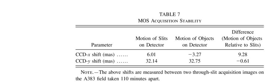 |
Note that the image motion of slits and objects in CCD‐y suggests uncorrected GMOS flexure that is a little larger than expected. We expect a peak of 2.2 μm hr−1 in CCD‐y (based on flexure measurements with GMOS on the telescope; Murowinski et al. 2003a, 2004), which corresponds to 12 mas hr−1. The value measured from the A383 acquisition images corresponds to 17 mas hr−1. However, the flexure compensation model currently in use at GMOS‐N is the one derived in the laboratory prior to shipping, and could be improved by rederiving the flexure model with GMOS mounted on the telescope.
This is of course only one example. Prior to shipping GMOS, comprehensive measurements were made of OIWFS flexure relative to the GMOS mask over a wide range of gravity vectors (Murowinski et al. 2003a). The worst‐case laboratory measurements of OIWFS flexure correspond to about 22 mas hr−1 in the CCD‐x direction, so it should not be necessary to recenter slit masks unless very narrow slits are used (e.g., 0 2). Introduction of an OIWFS flexure compensation model could improve this stability even further.
5.4. Example Multiobject Spectroscopic Data
MOS observations were taken through the A383 mask on 2001 August 26 and 27. Five 1800 s exposures were taken, using the B600 grating set to a central wavelength of 6000 Å (and no order‐sorting filter). The MOS data shown in Figure 7 represent the median of the three raw data frames from August 27.
All five frames were reduced using the Gemini IRAF package. The tasks and method used were the same as for the long‐slit case, extended to multiple slitlets. Flux calibration was done using a general B600 sensitivity function constructed using long‐slit observations of the spectroscopic standard stars G191B2B and BD 284211, taken with the B600 grating at several central wavelength settings.
An example of an extracted, wavelength‐ and flux‐calibrated spectrum from this mask is shown in Figure 9. This galaxy has r'(AB)∼18.8 (estimated from the GMOS preimaging using approximate zero points). For comparison, also shown is a 3600 s spectrum of the same galaxy obtained with the LRIS spectrograph (Oke et al. 1995) on the Keck 10 m telescope from the work of Smith et al. (2001). In the region of overlap, the same absorption features are seen in both spectra. The mean redshift and its uncertainty was measured from six absorption lines in the GMOS spectrum, and was found to be z = 0.1843 ± 0.0002. This agrees well with the value derived from the Keck spectrum (using four lines) of z = 0.1845 ± 0.0003.

Fig. 9.— Comparison of Gemini‐GMOS (lower spectrum) and Keck/LRIS (upper spectrum) observations of the same galaxy in the A383 cluster. The GMOS spectrum is extracted from the 2.5 hr of MOS data described in § 5.4. The LRIS spectrum is a 1.0 hr exposure from the work of Smith et al. (2001). The GMOS spectrum (dispersion 0.45 Å pixel−1) has been smoothed to approximately match the lower dispersion of the LRIS spectrum (2.55 Å pixel−1), and an arbitrary offset has been added to the Keck spectrum for clarity. The same absorption features are visible in both spectra in their region of overlap, and the GMOS spectrum confirms the redshift of this galaxy (z = 0.184, see text) with clear identification of the redshifted Ca H and K features at ∼4700 Å.
The GMOS data on A383 are currently being analyzed with the scientific goal of obtaining redshifts of galaxies in the field and of faint gravitational arc images. These will be used to better constrain the lens model for this cluster.
5.4.1. Spectral Stability and Wavelength Calibration
The precision and the necessary frequency of wavelength calibration is set by the stability of both object positions within the slits and image stability at the GMOS detector. As described above, and in detail in Murowinski et al. (2003a, 2004), the design of GMOS incorporates careful control of instrument stability, in particular flexure of the OIWFS relative to the mask, and active compensation of flexure between the mask and detector (Murowinski et al. 2003a).
From the series of MOS spectral frames taken on 2001 August 26, the shift in sky lines on the detector can be measured as a function of time. Eleven sky lines from around the full frame were selected and were found on average to shift in CCD‐x (the dispersion direction) by 0.44 pixels over a period of 1.73 hr (i.e., 0.25 pixels hr−1). This corresponds to a wavelength shift of 0.11 Å hr−1 with the B600 grating and gives a rough estimate of the level of precision that can be achieved if wavelength calibration is taken interspersed with the science data.
Although not a primary requirement, one of the design goals for GMOS was to be able to measure velocities to an accuracy of 2 km s−1 for all objects over the 55 × 55 field. The 2 km s−1 mode of GMOS has not yet been commissioned, but the A383 data can be used as a first on‐sky test of the stability of the Gemini‐GMOS system. To meet the 2 km s−1 stability goal requires a total image movement of less than 3.125 μm hr−1 in the dispersion direction (CCD‐x) at the GMOS detector. The spectral shift of 0.25 pixels hr−1 measured above corresponds to 3.4 μm hr−1. Therefore, in this, the only case that has been examined against the stability performance specification, the performance is within 10% of the goal.
Again, it should be stressed that the A383 data described above is only one example and leaves much unexamined parameter space where stability performance may be different; for example, observations at different air masses, temperature ranges, and gravity vectors. A full description of the error budget and expected high‐stability performance of GMOS as estimated from lab and on‐telescope measurements is given in Murowinski et al. (2003a, 2004). The conclusion of that analysis is that GMOS on Gemini–North is close to meeting the 2 km s−1 goal (to within about 10%, in agreement with the measurements above), but to reach its full potential some improvements should be made. Possibilities include improvement of the flexure compensation model for telescope conditions, and addition of a model to compensate for differential flexure between the OIWFS and slit mask. Even without these improvements, GMOS is believed to be one of the most, if not the most, stable Cassegrain multiobject spectrographs ever built for a large telescope.
5.5. MOS Acquisition Repeatability
Deep MOS observations are sometimes carried out using the same mask on several nights. Typically, offsets calculated using the acquisition script when the mask is first used give a very good starting point for the setup on subsequent nights. For example, during the queue run of 2004 December 18–25, eight observations were carried out on four different masks that had been previously used. On four of these occasions no additional offsets were needed in x, y, or rotation. The rms of additional offsets for the eight observations were Δx = 0025, Δy = 0004, and 0 009 in rotation.
6. TARGET ACQUISITION TIMES
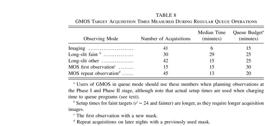
Target acquisition times have been measured in regular queue operations during the period of 2003 July to December. The setup time for imaging, long‐slit, and MOS modes are given in Table 8. Timing started at the beginning of the telescope slew and finished when science observations began. These times therefore include telescope slew time and occasionally also a pointing check and/or acquisition of a new sky‐background image for the OIWFS (if the sky background had changed significantly since the last sky image was acquired). Also included is the time taken for the OIWFS focus and astigmatism corrections to converge.
 |
In the case of imaging, GMOS is reconfigured during the telescope slew so that observations can begin as soon as the guiding, focus, and astigmatism corrections are stable. For long‐slit and MOS modes, there are additional steps involved to acquire the target(s) in the slit(s), as described in the relevant sections of this paper.
Although the measured setup times are a useful guide for visiting GMOS observers, it is important to note that the setup times budgeted when planning queue observations must be more conservative. This is needed in order to allow for extra acquisitions when the required observations of a target must be split over more nights than originally planned either to make the observations fit in the queue planning or to accommodate changing weather conditions. These queue budget times are given in column (4) of the table and should be assumed by users of GMOS in queue mode when planning their observations (these times are advertised on the Gemini Web pages). During queue operations, the setup time charged to a program is the actual time used (i.e., neither of the values shown in Table 8).
The observatory is continuing to monitor and reduce setup times. One area for potential improvement is more regular use of blind offsetting for acquisition of faint long‐slit targets. Additionally, it may be possible to reduce MOS acquisition times somewhat by reading out only small areas of the detector where the acquisition objects are located. Both of these will require modifications to the observation definition and acquisition software.
7. STANDARD CALIBRATION PROCEDURES
During GMOS queue operation, calibration data of various types are taken regularly and form a baseline calibration set that is sufficient for most programs. The frequency with which these calibrations are taken depends on the type of calibration. If a program requires special calibration that is not included in the baseline set, then these must be defined by the user (and the time taken to obtain any of these during the nighttime will be charged to the program). Below we describe the frequency and resulting accuracy of the baseline calibration set. The calibration procedures occasionally change, and users are advised to consult the GMOS Web pages for updates.
- Bad‐pixel mask.—These are derived from flats and bias images. They may be derived if/when changes in the detector array are found. The bad‐pixel mask for imaging mode will show the areas outside the imaging field of view as bad pixels, even though the pixels are not strictly bad; just not illuminated by the imaging field of view.
- Imaging flat field.—Twilight flats are taken each morning as the weather allows. All twilight flats from a 10–14 night run are distributed with imaging data obtained during the run. The typical noise in the average of the twilight flats obtained in a given run is 0.75%. Dome flats may also be taken, but are not guaranteed to be part of the baseline calibration set.
- Spectroscopic flat field.—GCAL flats are taken mixed with the science observations in long‐slit and MOS modes. A GCAL flat is obtained approximately once per hour of open shutter time (see § 4.2 on fringing), although a minimum of two are always obtained. For standard star observations, only one GCAL flat is obtained. This is sufficient, since the standard star observations have significantly higher signal‐to‐noise than most science observations. One twilight flat is taken per dark‐time run in which a MOS mask is used, weather permitting, with the instrument configuration (mask, grating, wavelength, and CCD binning) matching the science observations. These twilight flats can be used to derive the slit function for the mask. Twilight flats through long‐slits are only taken if the principal investigator requests them.
- Dark/Bias.—The dark current for the GMOS detectors is less than 1.0 e− hr−1, and hence dark images are normally not taken. Bias images are taken every night in the detector readout modes and binning settings used for the science observations. The bias is very stable, and all bias images obtained during a 10–14 night run can be used to create a high signal‐to‐noise bias image.
- Photometric standard stars.—Standard star fields are selected from Landolt (1992), and each GMOS observation of these fields contains three to five standard stars. A minimum of one field is observed each photometric night during which imaging programs are carried out, and is only obtained in the filters used for the science observations. Approximate zero points are also available from the Gemini Web pages. Nightly zero points give an accuracy of ∼0.05 mag (ignoring color terms) for objects with (r'−z')≤1.5, but for redder objects the color terms must be taken into account.Magnitudes in the SDSS system for all the Landolt standards are included in a calibration file in the Gemini IRAF package. Transformations from Smith et al. (2002) have been used to derive these magnitudes.
- World coordinate system.—This is automatically included in the header for each GMOS image. Relative accuracy is better than 01 on average over the field. Absolute accuracy is in most cases better than 5'' (but see § 5.1.1. for comments on this accuracy).
- Wavelength calibration.—One copper‐argon arc exposure matching the configuration (grating, filter, slit width, and CCD binning) is obtained once per dark‐time run that a spectroscopic science program is observed. Additional arcs are taken if necessary, for example if a grating has needed to be datumed (reset to the zero position). Arc exposures obtained at the elevation of the science observations are not included as part of the baseline calibration set. The accuracy of wavelength GMOS calibration taken during the day has been the subject of careful analysis based on lab measurements of GMOS flexure and grating and mask repositioning accuracy. The expected accuracy of daytime calibration is 0.6 pixels rms (Murowinski et al. 2004). This corresponds to different wavelength accuracy for the different gratings, but for example in the case of the B600 grating, this translates to 0.27 Å rms.
- Spectroscopic flux standards.—Spectrophotometric standard stars are selected from the sources listed on the Gemini Web pages. For each configuration (grating, filter, slit width, and CCD binning) used by a science program, a minimum of one spectrophotometric standard star is observed during each 10–14 night observing run when science data are taken for that program. Observations are not guaranteed to be obtained during the same nights as the science observations for the program. Standard stars are observed using the standard set of GMOS long‐slits. If a MOS program uses a nonstandard slit width, the standard star observations will be obtained through the long slit, with a slit width closest to the one used by the MOS program. Observations to provide absolute spectrophotometric calibration (e.g., wide‐slit observations) are not included as part of the baseline calibration set. The flux standard stars can also be used for approximate removal of telluric lines.
- Focal plane mask image.—Images of the long slits are obtained regularly for monitoring the quality of the slits. In addition, each MOS mask is imaged once using GCAL as the illumination source. These images are taken through the r'‐filter and are supplied as part of the baseline calibration set.
8. CURRENT STATUS OF GMOS
The first GMOS has been in regular science use on Gemini–North since 2001 November. At present the imaging, long‐slit, MOS, and IFU modes of GMOS‐N have been commissioned (see Allington‐Smith et al. 2002 for results of the latter). The atmospheric dispersion corrector has yet to be fitted and commissioned, and the high‐velocity precision (2 km s−1) mode has also not yet been commissioned.
A few changes have been made to GMOS since its arrival at Gemini–North. The cryostat has been fitted with a closed‐cycle cooler to replace the liquid nitrogen cooling system. Three new long‐pass filters have been purchased and fitted (GG455, OG515, and RG610), as well as new broadband filters (u' and a calcium triplet filter centered at 8600 Å) and a set of narrowband filters. More gratings have now been purchased: both B1200 and R600 are now available, although only three gratings can be mounted in the instrument at any time. Finally, the "nod‐shuffle" observing mode for accurate sky subtraction (Glazebrook & Bland‐Hawthorn 2001) has also been implemented. For details of the current status of GMOS and the complement of filters and gratings, see the Gemini/GMOS Web pages.3
We thank the staff at the Gemini–North Observatory for their support and hospitality during the commissioning period, and for their continued dedicated support of GMOS during community use. We also thank Jean‐Paul Kneib and Graham P. Smith for supplying reduced Keck data on the A383 galaxy shown in Figure 9. R. L. D. thanks PPARC for the award of a senior fellowship. We also thank the referees of this paper for helpful comments.
This paper is based on observations obtained at the Gemini Observatory, which is operated by the Association of Universities for Research in Astronomy, Inc., under a cooperative agreement with the NSF on behalf of the Gemini partnership: the National Science Foundation (US), the Particle Physics and Astronomy Research Council (UK), the National Research Council (Canada), CONICYT (Chile), the Australian Research Council (Australia), CNPq (Brazil), and CONICET (Argentina).
Footnotes
- 2
IRAF is distributed by National Optical Astronomy Observatories, which is operated by the Association of Universities for Research in Astronomy, Inc., (AURA), under cooperative agreement with the National Science Foundation. The Gemini IRAF package is distributed by Gemini Observatory, AURA.
- 3
Gemini/GMOS Web pages are at http://www.gemini.edu.