
ABSTRACT
The best ground‐based astronomical sites in terms of telescope sensitivity at infrared and submillimeter wavelengths are located on the Antarctic Plateau, where high atmospheric transparency and low sky emission are obtained because of the extremely cold and dry air; these benefits are well characterized at the South Pole station. The relative advantages offered by three potentially superior sites, Dome C, Dome F, and Dome A, located higher on the Antarctic Plateau, are quantified here through the development of atmospheric models using the line‐by‐line radiative transfer model code. In the near‐ to mid‐infrared, sensitivity gains relative to the South Pole of up to a factor of 10 are predicted at Dome A, and a factor of 2 for Dome C. In the mid‐ to far‐infrared, sensitivity gains relative to the South Pole up to a factor of 100 are predicted for Dome A and 10 for Dome C. These values correspond to even larger gains (up to 3 orders of magnitude) compared to the best mid‐latitude sites, such as Mauna Kea and the Chajnantor Plateau.
Export citation and abstract BibTeX RIS
1. INTRODUCTION
Astronomical sites for infrared and submillimeter astronomy require low sky emission and high atmospheric transmission; such conditions are found at sites on the high Antarctic Plateau. The extremely low temperatures throughout the Antarctic troposphere reduce the thermal emission from the sky. The low atmospheric temperatures prevent the atmosphere from containing significant amounts of water vapor (Lane 1998). As atmospheric absorption throughout the far‐infrared and submillimeter is dominated by molecular water vapor, a number of windows are opened up that cannot be accessed elsewhere.
Experimental data taken with a number of instruments have shown that the wintertime atmospheric thermal emission above the South Pole station is significantly lower than that found at any other ground‐based site. These instruments include the GRIM (a near‐infrared grism spectrometer) on the SPIREX telescope (Herald 1994), the Infrared Photometer Spectrometer (Ashley et al. 1996; Phillips et al. 1999), the Mid‐Infrared Sky Monitor (Chamberlain et al. 2000), the Near‐Infrared Sky Monitor (Lawrence et al. 2001), and a Michelson‐type interferometer (Walden et al. 1998). These instruments cover the 1.5–20 μm waveband and have shown a reduction in emission compared with mid‐latitude sites by up to an order of magnitude in the mid‐infrared and up to 2 orders of magnitude in the near‐infrared.
Aerological data from radiosonde balloons have shown that the South Pole average wintertime precipitable water vapor (PWV) column density is 250 μm (Chamberlin 2001). This is significantly lower than that found at good‐quality mid‐latitude sites such as Mauna Kea (1.6 mm average in winter) and the Chajnantor Plateau (1 mm average in winter; Lane 1998). The resulting decrease in atmospheric opacity and increase in stability has been experimentally confirmed by several instruments: the UNSW SUMMIT (Calisse et al. 2004) and the NRAO/CMU submillimeter tipper (Peterson et al. 2003), both 350 μm radiometers; and the AST/RO telescope operating at 610 μm and 1300 μm (Stark et al. 2001).
Moderate‐resolution atmospheric models of the South Pole sky emission and transmission (produced from the MODTRAN atmospheric code) throughout these wavebands have been published by Hidas et al. (2000), Chamberlain et al. (2000), and Bally (1989). A higher resolution model (using the line‐by‐line radiative transfer model; LBLRTM) has been reported by Walden et al. (1998). These atmospheric models are based on input aerological data from radiosonde balloons measuring profiles of pressure, temperature, water vapor content, and ozone. These data have been collected from the South Pole station since 1956 and are publicly available. The atmospheric models have shown good quantitative agreement with experimental observations (Walden et al. 1998).
The US South Pole station (0° east, 90° south, 2835 m elevation) is the most well characterized site on the Antarctic Plateau. While the benefits of its low sky background are well recognized, and the unique atmospheric turbulence profile is potentially beneficial for some applications (Lawrence 2004; Lloyd et al. 2002), the ground‐level seeing is relatively poor (1  8 in the visible) compared with quality mid‐latitude sites. However, there are several other sites on the Antarctic Plateau that are potentially superior. These include the established Russian and Japanese winter‐capable stations, Vostok (107° east, 78° south, 3500 m elevation) and Dome Fuji (40° east, 77° south, 3810 m elevation); the French/Italian station currently under construction, Dome C (123° east, 75° south, 3260 m elevation); and the highest point on the plateau, Dome A (74° east, 81° south, 4200 m elevation). The advantages of these higher plateau sites arise from their higher altitudes—which should result in lower atmospheric temperatures and lower water vapor content (Marks 2002)—and their local topography; as the three "domes" lie on high points of the plateau, the ground‐level turbulence driven by local inversion winds is expected to much lower than that found at the South Pole (Gillingham 1993).
In the current paper the atmospheric emission and transmission of three of these high‐plateau sites (Dome C, Dome F, and Dome A) are modeled based on temperature, pressure, and water vapor profiles. Wintertime radiosonde measurements have been reported from the South Pole over many seasons1 and from Dome Fuji in 1997 (Hirasawa et al. 1999). The only data available from Dome C have been taken over summer, and the station is not due for winter operation until 2005. No data currently exist from Dome A. The aerological profiles for these two sites are thus inferred from characteristics of South Pole and Dome Fuji radiosondes and automatic weather station (AWS) data. The atmospheric models are then applied to determine the relative benefits of the high‐plateau sites in terms of the sensitivity of infrared and submillimeter telescopes placed there, compared to standard mid‐latitude sites.
The impact of the atmosphere on telescope sensitivity is just one of many factors that must be considered to determine the quality of a particular astronomical site. Other important parameters include the percentage of photometric nights, the total integrated turbulence (and its low‐ and high‐altitude components), the ground wind speed statistics, the high‐altitude wind speed, the ground temperature, the seismic activity, the amount of rainfall and snowfall, the level of atmospheric dust and aerosols, communications infrastructure, logistics, accessibility, and political stability. Although evidence exists to suggest that favorable conditions for many of these factors will be found at Dome C, this must be weighed against any disadvantages arising from the extreme conditions or the remoteness of the site.
All models used here consider observation at zenith. The actual air mass will depend on the type of observation, and there are advantages and disadvantages to both mid‐latitude sites and high latitude Antarctic sites. For example, mid‐latitude sites offer advantages because a larger region of the Galactic plane passes through the zenith, whereas high‐latitude sites offer benefits because longer observations are possible at the same air mass.
2. ATMOSPHERIC MODELS
2.1. Input Model Parameters
The LBLRTM atmospheric code is used here to model four Antarctic atmospheres. This code outputs emission and transmission spectra based on input vertical distributions of atmospheric properties and components. The most important for infrared/submillimeter wavelengths are pressure, temperature (discussed in § 2.2), water vapor (discussed in § 2.3), and ozone. The LBLRTM code also allows input from many trace molecular components, such as nitrous oxide, methane, and carbon dioxide. Because of the very low pressures and temperatures in the higher stratospheric layers, altitudes above ∼60 km do not significantly impact on the atmospheric emission and transmission characteristics at the resolution of interest and are ignored in the following analysis.
The wintertime pressure profile is determined from an average of South Pole radiosonde balloon launches. It is well known that the atmospheric pressure is lower on the Antarctic Plateau; i.e., the "physiological altitude" at a given height above sea level on the Antarctic Plateau is higher than that observed at mid‐latitudes. This is due to the extreme cold temperatures above the continent. Significant differences in the pressure profile with altitude across the plateau are not expected. The same pressure profile is thus used for each of the Antarctic sites examined, with the ground level set to the appropriate altitude.
The input South Pole ozone profile is taken from a number of South Pole mid‐winter ozonesondes.2 These are averaged and then scaled to give a column density of 250 Dobson (the average South Pole mid‐winter value). This is known to drop to as low as 100 Dobson in late spring, which may have a significant effect in some regions of strong ozone absorption, such as at ∼9 μm. The effect is not modeled here, however, as the wintertime value is quite stable from year to year. Because the majority of atmospheric ozone is confined to stratospheric layers centered around 15 km in altitude, the same profile is used for each of the four Antarctic sites.
Nitrous oxide, methane, carbon dioxide, and carbon monoxide profiles for the South Pole during winter published by Walden et al. (1998) are used for the current South Pole model. There is little change in these molecular abundances for heights lower than a few kilometers. The same profiles are thus used for each of the four Antarctic sites. Aerosol content for each of the Antarctic atmospheres is modeled as described by Hidas et al. (2000).
2.2. Temperature Profiles
Figure 1 shows the average temperature profile observed above the South Pole station from 3 months in winter of 1997 representing 58 balloon radiosondes.3 This profile is characteristic of the mid‐winter South Pole atmosphere. The ground temperature is close to the average value of −61°C recorded by AWSs over this period.4 A negative temperature lapse rate extends above the surface to an altitude ∼300 m above the ground, where the temperature is some 22°C warmer. The strong adiabatically stable surface inversion layer results from the long winter period of surface radiative cooling. This is followed by a wide isothermal layer that extends up to ∼1–2 km where the free atmosphere begins. Above this surface boundary layer, the temperature falls off throughout the troposphere until the isothermal tropopause layer (∼7 km above ground level). The temperature then continues to drop throughout the lower stratosphere.
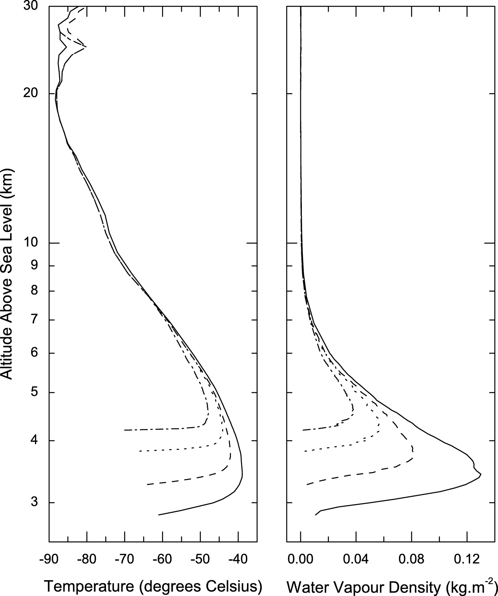
Fig. 1.— Temperature profiles (left plot) and water vapor density profiles (right plot) for the model atmospheres. The South Pole (solid line) and Dome Fuji (dotted line) profiles represent averages from radiosonde balloon launches. The Dome C (dashed line) and Dome A (dash‐dotted line) profiles are interpolated/extrapolated from these (see text).
The average temperature profile from the Dome Fuji station over the same 3 month period in 1997 (representing 55 balloon launches from Hirasawa et al. 1999) is also shown in Figure 1. The ground‐level temperature for this profile is set to the average ground‐level temperature recorded by AWS5 over this period (−66°C), as there is some uncertainty in the lowest altitude balloon readings. Similar to the South Pole atmosphere, a strong surface inversion layer is observed. However, this is confined significantly closer (∼100 m) to the ground. This reduction in inversion layer height has been predicted to occur at such sites (Dopita et al. 1996; Marks 2002) as a results of the local topography. A general characteristic of the nocturnal adiabatically stable inversion layer at any site is that the height scales with the magnitude of the ground‐level winds, the magnitude of the geostrophic winds resulting from the Coriolis force at altitudes 1–2 km above the surface, and the relative direction of these two winds (Kaimal & Finnigan 1994). On the Antarctic Plateau two components contribute to ground‐level winds: inversion winds due to local surface slopes, and katabatic winds originating from such inversion winds at higher sites.
At the South Pole, these factors combine to generate an average wind speed of 6.3 m s−1, which is predominantly directed from the high‐plateau sites.6 On the domes, however, the local inversion winds should be much lower (because of the extreme ground‐level flatness), and the katabatic winds should lose energy in proportion to the altitude of the dome with respect to the origin of the winds. Thus, very low wind speeds are recorded at Dome C (2.8 m s−1 average, 2.6 m s−1 50% quartile over 8 yr) and Dome F (2.6 m s−1 average, 2.2 m s−1 50% quartile recorded over 6 yr).7 The wind speed averages for Dome C are somewhat higher than reported by Valenziano & Dall'Oglio (1999), probably as a result of differences in binning (C. Meyer et al. 2004, in preparation). For Dome Fuji, 1 year of the 6 available shows unusually high average wind speeds; neglecting this anomalous year from the analysis gives 2.2 m s−1 average and 2.0 m s−1 50% quartile wind speed, which is probably more representative of long‐term trends. At Dome A, still lower wind speeds should be encountered. It is therefore expected that the boundary layer height will decrease with the altitude of the site, as confirmed by the Dome Fuji observations.
The free atmospheric temperature profile from ∼2 km above the Dome Fuji surface is similar to that observed above the South Pole, despite the large distance (∼1400 km) between the two sites. Good agreement (within 2°) is also observed with wintertime upper tropospheric temperature profiles recorded at the Vostok station (V. Lukin, 2003 Russian Antarctic Expedition, private communication). This uniformity of the upper Antarctic Plateau troposphere occurs because of the significant height of the plateau above sea level, the length of the Antarctic winter, and the persistence of the Antarctic polar vortex (a low‐pressure system circumnavigating the continent), which acts to isolate the plateau troposphere from mixing with warmer air at higher latitudes.
Based on the characteristics of the two experimental temperature profiles for South Pole and Dome Fuji, models for the wintertime Dome C and Dome A profiles have been derived. These are shown in Figure 1. For Dome C the ground temperature is set to the average value recorded over this 3 month period. Extrapolating temperatures recorded at these three sites (and from the Vostok station) gives an average temperature ∼10° colder at the altitude of Dome A, as shown in Figure 2. The point at which the temperature lapse rate begins to increase (after the isothermal surface layer) toward its tropospheric (free atmosphere) rate is assumed to occur at 1.5 km above ground level, as observed at Dome Fuji. The free atmosphere above this level is assumed to be equal at each of the four sites. Interpolation/extrapolation is used to set the surface inversion layer height for each site (to 200 m for Dome C and 50 m for Dome A, compared with 300 m for the South Pole and 100 m for Dome Fuji), based on the assumption that the average ground wind speed and hence inversion layer height is decreasing as the altitude increases. The maximum surface inversion layer temperature is then determined from these two factors (height of inversion layer and height of free atmosphere).
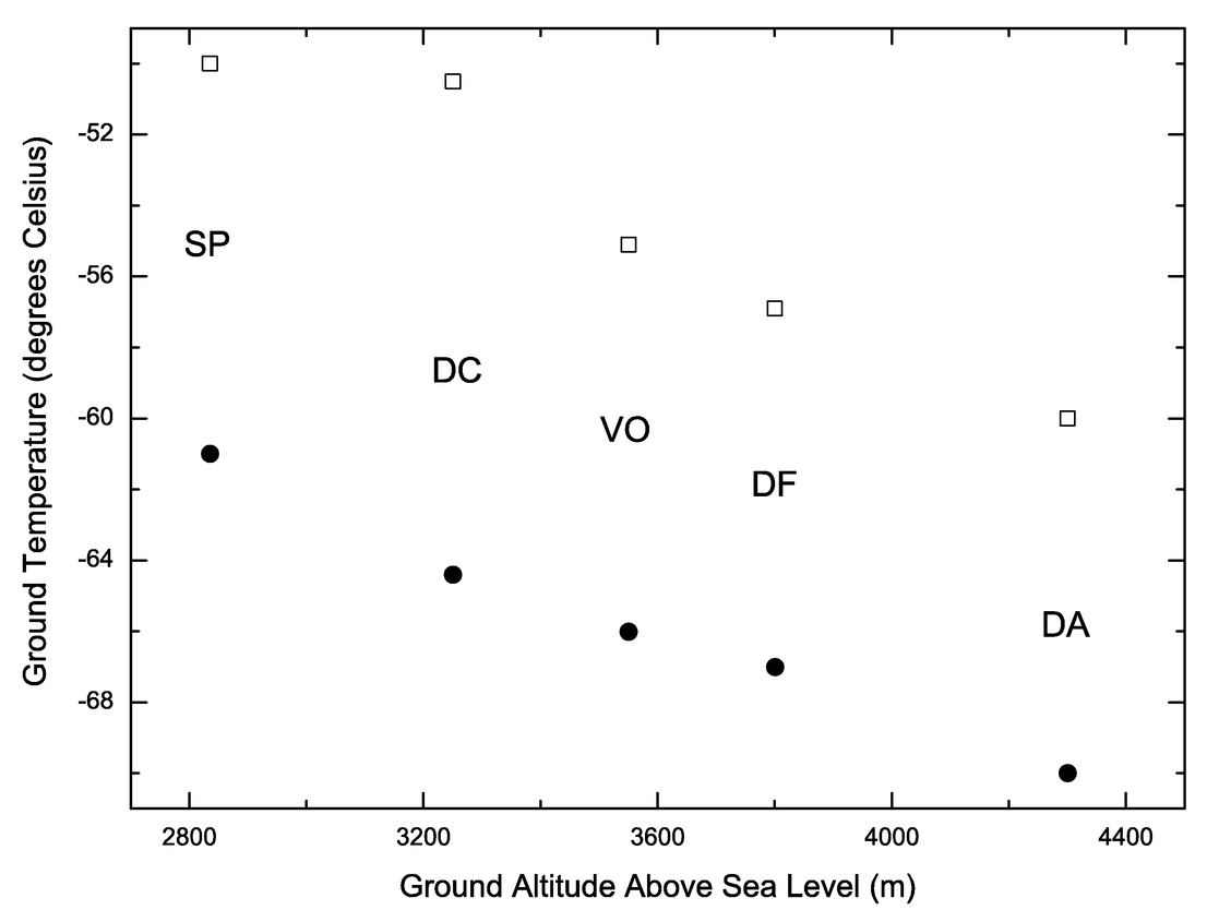
Fig. 2.— Average ground temperature for several sites on the Antarctic Plateau, recorded from Automatic Weather Stations. Yearly (open squares) and wintertime (filled circles) average values are shown for the South Pole (SP), Dome C (DC), Vostok (VO), and Dome Fuji (DF). The values for Dome A (DA) have been extrapolated from these.
It should not be expected that the Dome F and South Pole profiles represent a thorough long‐term statistical mean. In addition, there is a large uncertainty in the derived Dome C and Dome A profiles, primarily because the assumed relationships between site altitude and ground wind speed, ground‐level temperature, and boundary layer height will probably not be linear. However, these profiles should give a generally representative comparison of the four sites, which is the goal of this paper.
2.3. Water Vapor Profiles
Chamberlin (2001) has shown that the 50% quartile South Pole wintertime PWV content is 250 μm, which is typically 70%–90% of the saturated PWV content (with respect to the water vapor partial pressure over ice). The saturated PWV content for the South Pole average temperature profile shown in Figure 1 is 330 μm. The average value of the relative humidity profile (recorded for each of these balloons) gives a PWV content of 255 μm (close to the average value), representing ∼80% saturation. The water vapor density distribution calculated from this relative humidity profile is shown in Figure 1.
Also shown in Figure 1 is the water vapor density distribution calculated from the Dome Fuji data (Hirasawa et al. 1999). Although a reduced data set has yet to be made publicly available, preliminary analysis shows that on average the atmosphere is ∼60% saturated during the coldest winter months. The saturated value for the average temperature profile is 175 μm, which results in an average water vapor content of ∼105 μm.
Summertime radiosonde and photometric measurements from Dome C (Valenziano 1998; Valenziano & Dall'Oglio 1999) show a PWV value similar to that observed at the South Pole during the summer months (500–600 μm). This does not indicate that the wintertime values at the two sites should be similar, however, as evidenced by radiosonde observations from the Vostok station (Burova et al. 1986; Townes & Melnick 1990), which also shows summertime values similar to the South Pole (500 μm), but a winter average (200 μm) that is ∼80% of the South Pole winter 50% quartile value.
Although a complete temperature profile is not available from the Vostok station, the altitude of the site indicates that the reported PWV values represent an average relative humidity similar to the 70%–90% observed at the South Pole. The significant reduction in average relative humidity observed at Dome Fuji, therefore, must be attributed to topographic differences between the two sites. As the katabatic winds originate at the domes, these may act to transfer humid air from the high sites to the lower sites such as the South Pole. It is thus expected that the average relative humidity at Dome C lies somewhere between the South Pole (80%) and Dome Fuji values (60%), and that the relative humidity at Dome A will be lower still. The saturated PWV content from the derived Dome C temperature profile is 235 μm. Choosing the midpoint of the (South Pole and Dome F) relative humidity values then gives a PWV of 160 μm. For Dome A the thermal profile gives a saturated PWV content of 120 μm. Two models for the Dome A PWV are developed, with a average relative humidity of 50% (giving a PWV content of 60 μm) and 25% (giving a PWV content of 30 μm). The water vapor distributions for these models are shown in Figure 1.
As with the temperature profiles, there is significant uncertainty in the derived water vapor distributions for Dome C and Dome A. In addition, there is some uncertainty about the validity of the operation of relative humidity sensors at very low temperatures. From the data sets available from the South Pole, Dome Fuji, and Vostok, the water vapor content of the atmosphere shows a significant standard deviation. Average monthly values as low as 60 μm have been recorded at Vostok, and values as low as 40 μm at Dome Fuji. Even if the assumptions about relative humidity at Dome C and Dome A are incorrect and the atmospheres are completely saturated, this still gives a PWV value significantly lower than that observed at the South Pole, and the average values based on relative humidity estimates should be observed for some fraction of the time.
2.4. Mid‐Latitude Profiles
In order to make comparisons with mid‐latitude sites three further atmospheric models are developed. For observations in the visible and near‐ to mid‐infrared, the site at Mauna Kea (155° west, 19° north, 4200 m elevation) on the island of Hawaii is characteristic of a very good quality mid‐latitude site. For submillimeter‐to‐millimeter observations, the best mid‐latitude sites currently found lie in the Chajnantor Plateau region (68° west, 23° south, 5000 m elevation) of northern Chile, where the air is significantly drier than that found above Mauna Kea. Mid‐latitude observations of wavelengths between these two regions (in the mid‐ to far‐infrared) require an even higher telescope site to further reduce atmospheric water vapor absorption. This is the motivation for the planned airborne telescope SOFIA (Stratospheric Observatory For Infrared Astronomy).
The Mauna Kea model used here is based on a radiosonde balloon temperature profile launched from the summit (Bely 1987) and surveying the first 6 km of the atmosphere. The upper tropospheric temperature (and pressure) is obtained from radiosondes launched at the sea level site of Hilo (approximately 20 km from Mauna Kea). Analysis has shown that the free atmosphere several hundred meters above the summit is in good agreement with the free atmosphere recorded from the Hilo site. The relative humidity from the Hilo radiosonde data is scaled to give a PWV content of 1.6 mm, representing the 50% quartile value in wintertime (Lane 1998). Ozonesondes are also regularly launched from the Hilo site. An ozone profile giving a column density of 280 Dobson (the average winter value) is chosen for this model.
Chajnantor and Mauna Kea lie at similar latitudes (in opposite hemispheres). It is thus assumed that the free atmospheric temperatures are similar, in agreement with published lower troposphere profiles from the Chajnantor Plateau (Giovanelli et al. 2001). The main difference in the Chajnantor site is the lower water vapor content, which is scaled in the model to give a PWV of 1 mm, representing 50% quartile wintertime conditions (Lane 1998). Following the analysis of Hidas et al. (2000), the aerosol content for these two sites is modeled with a reduced visibility component compared to the Antarctic sites.
For both the Mauna Kea and Chajnantor sites, the LBLRTM standard geographical‐seasonal model for a mid‐latitude winter site is used for distribution of trace molecules. For the airborne observatory model, the mid‐latitude winter model is used for all atmospheric profiles, with the ground level raised to the standard flight altitude of 14 km and the water vapor content scaled to give a PWV of 10 μm (Giovanelli et al. 2001).
3. ATMOSPHERIC EMISSION
The near‐ and mid‐infrared sky emission spectra for the South Pole and Mauna Kea models are shown in Figure 3. For reference the emission from a 5% emissive telescope is shown at 0°C and −61°C. The Manua Kea sky background is shown to be a factor of 80 brighter than the South Pole background at the edge of the K‐dark band (2.4 μm), a factor of 10–20 in the L band (3.8 μm), a factor of 5–10 in the M band (5 μm), a factor of 4–8 in the M' band (8.5 μm), and a factor of 2–5 in the N band (10–14 μm). Good correlation is found between these relative values with ratios calculated from published near‐infrared Mauna Kea theoretical spectra8 and experimental data,9 experimental mid‐infrared Mauna Kea spectra (Chamberlain et al. 2000), and South Pole experimental data (Chamberlain et al. 2000; Smith & Harper 1998; Walden et al. 1998). Although the model predictions of the emission ratios between the two sites agree with experimental observations, the emission fluxes in the K‐dark window, for each atmosphere, are somewhat lower than experimentally observed. This probably occurs because residual airglow emission is neglected in the models. Figure 3 also demonstrates the importance of telescope emission, which dominates both South Pole and Mauna Kea sky emission throughout the M band and begins to dominate the Mauna Kea sky emission for shorter wavelengths (towards the K band). If the telescope emission is reduced to less than 1%, then the atmospheric signal dominates in all wavelengths for each of the atmospheres.
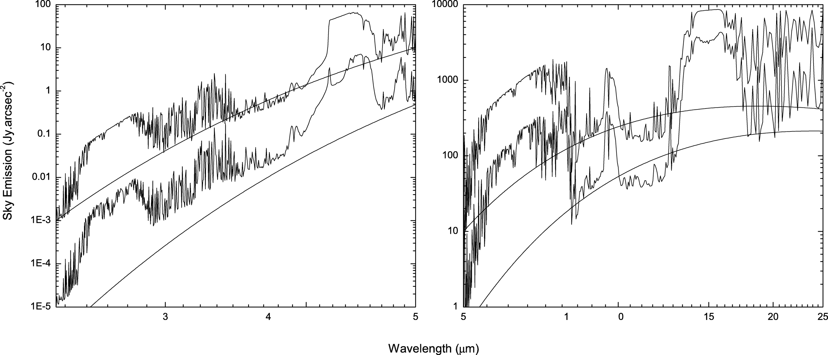
Fig. 3.— Model wintertime sky emission in the near‐ and mid‐infrared for Mauna Kea (top curve) and the South Pole (bottom curve). The emission from a 5% emissive telescope at ground temperatures of −60°C and 0°C are also shown.
The sky emission B for each of the four Antarctic sites is compared in Figure 4, which shows the emission ratios BSP/BDC, BSP/BDF, and BSP/BDA. As expected, the lower atmospheric temperatures of the high‐plateau sites generate a lower atmospheric emission. The magnitude of this reduction is highest for each site in the near‐infrared, where the Planck function is steepest at these atmospheric temperatures. The Dome A atmosphere is a factor of 4–8 darker in the K and L' bands, and a factor of 3 darker in the L band. In the mid‐infrared, the Dome A site should be twice as dark as the South Pole site in transparent regions. The model predicts only a modest reduction in sky brightness at Dome C; from 1.5 at lower wavelengths to 1.2 at longer wavelengths. Summertime data from Dome C (Walden & Storey 2004) has shown that the mid‐infrared (6–15 μm) sky emission is approximately equivalent to the South Pole sky emission in winter. The summer and winter South Pole sky emission have also been compared by Walden et al. (1998), who found a difference of ∼1.2. This would indicate that the Dome C winter emission should be at least this factor lower, which agrees with the current model.
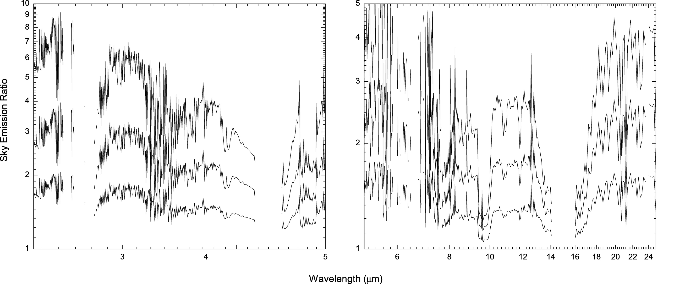
Fig. 4.— Ratio of South Pole near‐ and mid‐infrared sky emission to Dome C (bottom curve), Dome Fuji (middle curve), and Dome A (top curve) sky emission.
Figure 5 compares mid‐infrared sky emission from 27 to 50 μm. Shown are the emission ratios BCP/BSP, BCP/BDC, BCP/BDF, and BCP/BDA. The emission for each Antarctic site is similar in opaque regions of strong water vapor absorption, and this is a factor of ∼1.4 lower than the Chajnantor Plateau emission. In transparent regions the emission is strongly dependent on the atmospheric PWV content—low water vapor absorption results in emission originating from higher, hence colder, regions of the atmosphere. This same effect is observed throughout the far‐infrared and submillimeter, but the emission ratios are reduced as the blackbody function gradient decreases.
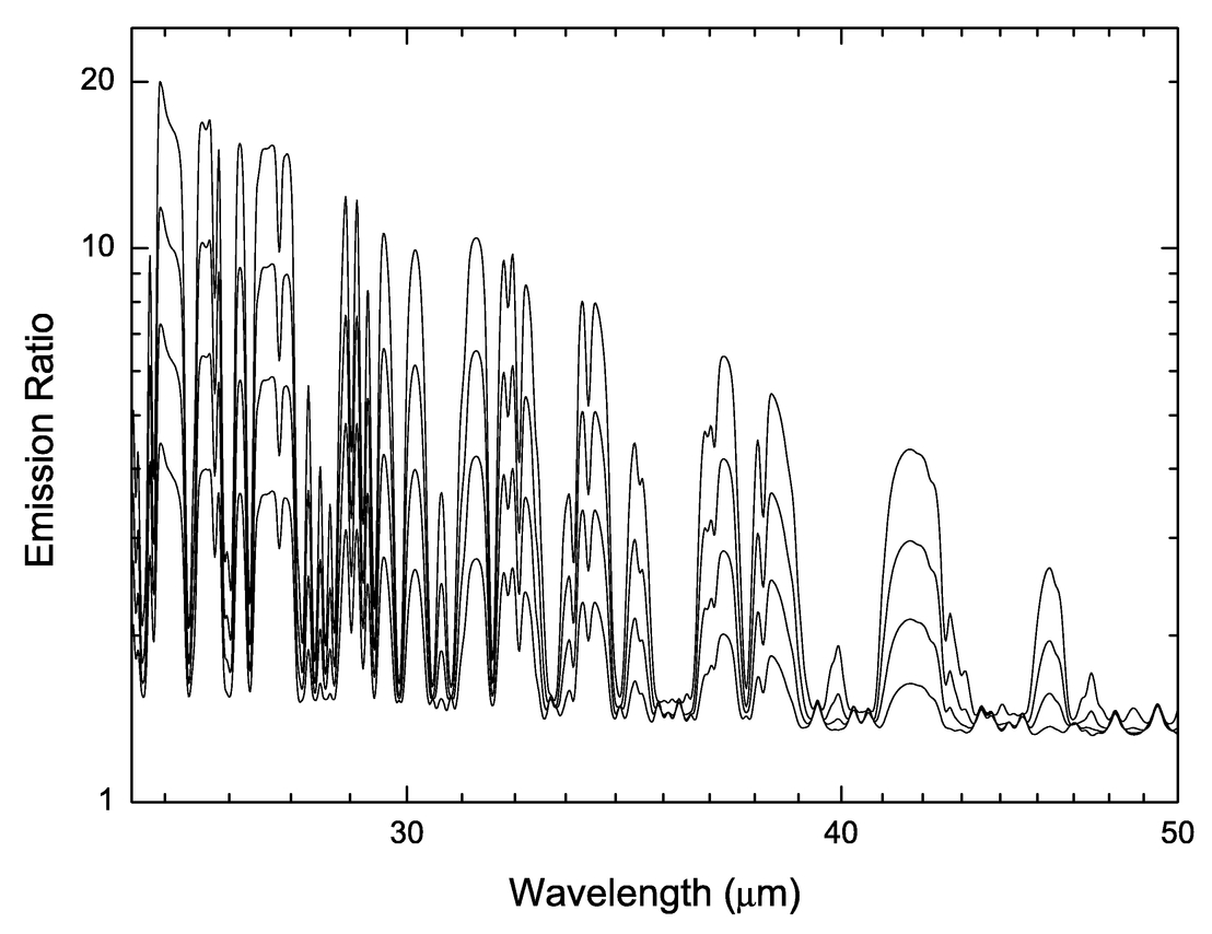
Fig. 5.— Ratio of Chajnantor Plateau mid‐infrared sky emission to South Pole (bottom curve), Dome C, Dome Fuji, and Dome A (top curve) sky emission.
4. ATMOSPHERIC TRANSMISSION
The atmospheric transmission in the near‐ and mid‐infrared is characterized by a number of molecular absorption bands, including water vapor at 2.5, 3.1, 6, and 25 μm, ozone at 9.7 μm, carbon dioxide and oxygen at 4.3 and 15 μm, respectively, and methane and nitric oxide at 7.6 μm. The primary advantage of the Antarctic sites, in terms of transmission, occurs at wavelengths of strong water vapor absorption, as the difference in abundance of other absorbing molecules is less significant. The Mauna Kea transmission spectrum is compared with the Dome A (best conditions) model over the near‐ to mid‐infrared (2.4–27 μm) region in Figure 6. The most notable increase in atmospheric transmission for the plateau sites is observed at the edges of standard infrared bands, particularly K', L, M, and Q, which become much cleaner at the high Dome A site.
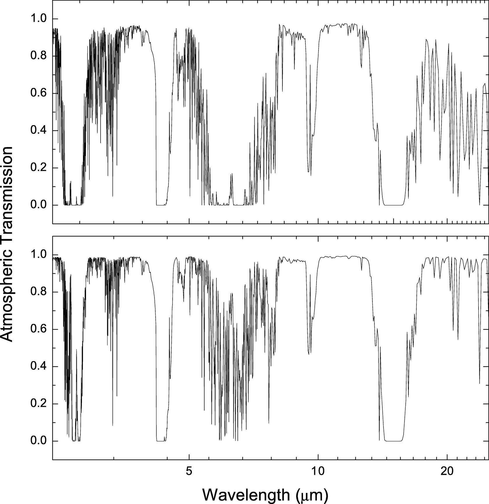
Fig. 6.— Atmospheric transmission in the near‐ and mid‐infrared for Manua Kea (top graph) and Dome A (bottom graph).
For observations longward of ∼20 μm, the transmission is almost entirely determined by water vapor absorption bands. Figure 7 compares the atmospheric transmission from the mid‐infrared to submillimeter for the Chajnantor Plateau, the South Pole, Dome C, Dome Fuji, Dome A (both models), and SOFIA. Despite the very low PWV content of the Chajnantor Plateau atmosphere compared with other mid‐latitude sites, the atmosphere is almost completely opaque throughout this wavelength region. There are only a few windows (around 28, 350, and 450 μm) for which observations can be attempted. It is well known that the South Pole experiences a considerable increase in transmission at these windows and that a number of others become accessible (most notably 200, 225, and a series below 40 μm). This figure shows the extraordinary benefits of moving from the South Pole to the higher plateau sites. At Dome A under the best conditions, ∼75% of this (25–500 μm) window is above 20% transmissive, whereas less than 15% of this window is above 20% transmissive at Chajnantor Plateau. The Dome A site is still opaque at absorption line centers; however, in clear windows the transmission is a relatively high fraction of the transmission of a high‐altitude airborne observatory.
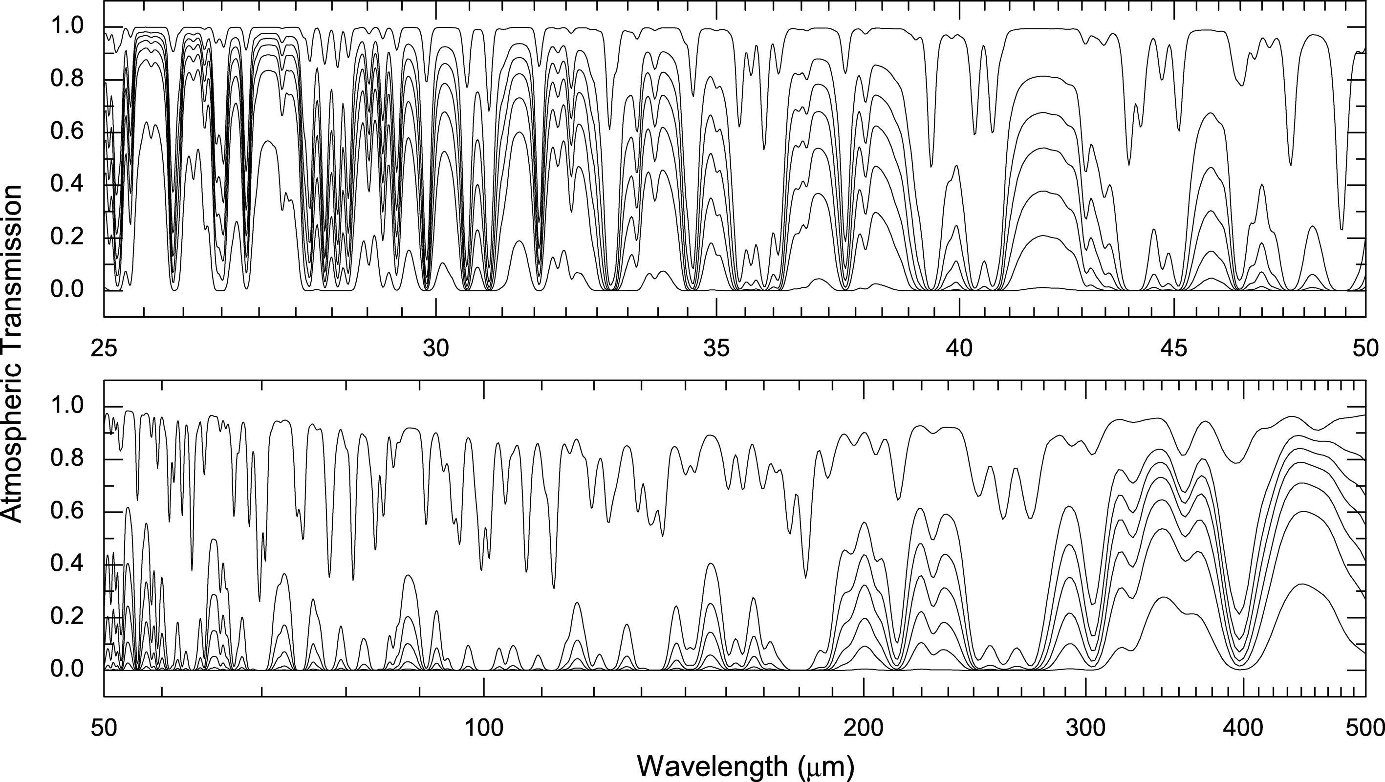
Fig. 7.— Atmospheric transmission in the far‐infrared/submillimeter. The plot shows, in order of increasing transmission at any wavelength, Chajnantor Plateau, the South Pole, Dome C, Dome Fuji, Dome A (average conditions), Dome A (good conditions), and SOFIA. The PWV content for each model atmosphere is 1000, 250, 175, 105, 60, 30, and 10 μm, respectively.
There is some disagreement between the opacities determined by numerical models and those determined by experimental observation in the submillimeter region (Pardo et al. 2001). A continuum‐like submillimeter "dry air" opacity has been attributed principally to far wings of higher frequency water lines. Although the LBLRTM code includes such a term, and a South Pole model with zero water vapor does generate a nonzero opacity at submillimeter wavelengths, there may be some error in the magnitudes of transmission at the longer wavelengths. Peterson et al. (2003) give an average opacity τ at 350 μm of 1.20 and 1.39 for the South Pole and Chajnantor, respectively. Correcting these to narrowband values (Calisse 2004) gives transmissions (and transmission ratios) that agree with the current model predictions within ∼15%.
5. TELESCOPE SENSITIVITIES
A useful metric for the comparison of infrared sensitivities at different sites is the ratio of integration times required to give a specific signal‐to‐noise ratio at a given stellar magnitude (e.g., Lloyd‐Hart 2000). For point‐source observations, this can be expressed as
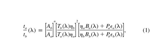
where A is the telescope area, T is the atmospheric transmission, B is the sky background,  is the telescope emissivity, P is the ground temperature blackbody emission, η is the telescope optical transmission, the power index n = 1 for seeing‐limited observations and n = 2 for diffraction‐limited observations, and the subscripts a and b refer to the two sites being compared. This equation considers that the thermal background dominates the signal and the detector noises, and ignores the confusion limit. It considers that the detector efficiency and gain and the spectral resolution for the two telescopes are the same; it also assumes that the focal plane is sampled at Nyquist frequency and that (for seeing‐limited conditions) the seeing is the same at the two sites being compared.
Figure 8 compares the sensitivities of equivalent telescopes (same collecting area, emissivity, transmission, and [diffraction‐limited] spatial resolution) located at the South Pole with each of the high‐plateau sites, from the near‐infrared to the submillimeter. In transparent regions of the near‐ and mid‐infrared (up to ∼20 μm), the gains offered by the higher plateau sites are consistent with the decrease in sky spectral brightness (an improvement of 20%–80% in sensitivity is gained at Dome C, and 200%–400% at Dome A). In less‐transparent regions at the edges of absorption bands (centered around 2.7 and 7 μm), the decrease in emission combines with the increase in transmission to generate a substantial benefit for the high‐plateau sites (a factor of 2–3 for Dome C and 10–20 for Dome A), which should allow these wavelengths to be examined considerably better than at temperate latitudes.
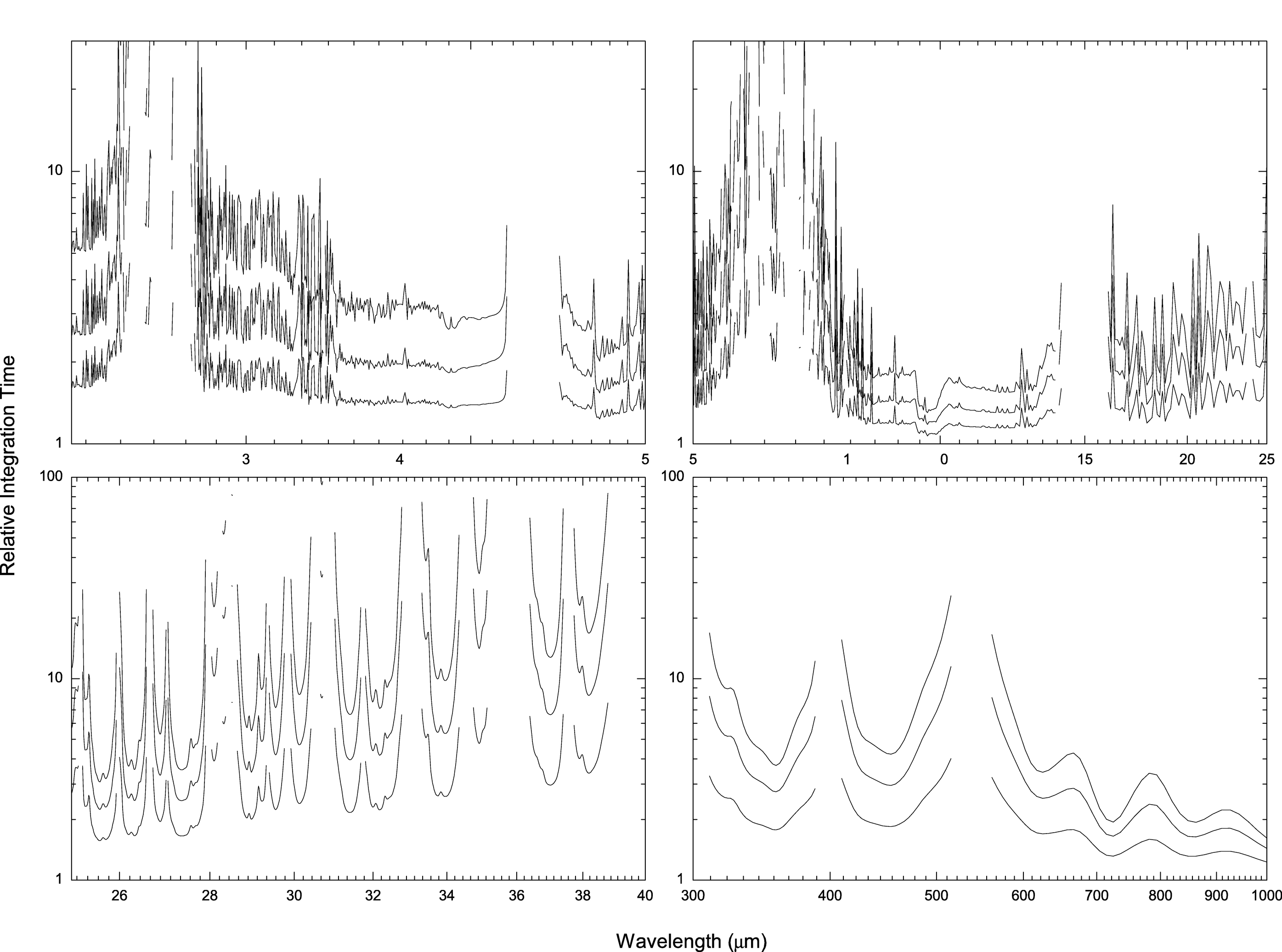
Fig. 8.— Ratio of integration times from the near‐infrared to submillimeter for a South Pole telescope compared with a Dome C (bottom curve), Dome F (middle curve), and Dome A (top curve) telescope. Each telescope is assumed to be diffraction‐limited and equivalent in all aspects. Values are only shown for wavelengths at which the South Pole transmission is greater than 10%.
At wavelengths longer than about 20 μm, the relative integration time is influenced primarily by the sky transmission rather than emission. For observations up to ∼40 μm, large gains are observed for all wavelengths (not just opaque regions). An improvement by a factor of 2–8 is expected at Dome C, and 10–100 for Dome A. In the submillimeter (longward of ∼200 μm), the advantages offered in Antarctica are well understood and have resulted in a number of telescopes being built (Stark et al. 2001) and proposed at the South Pole. However, as shown in Figure 8, the higher plateau sites could offer significant advantages at the longer wavelength end. At wavelengths between these two regions (40–200 μm), a quantitative comparison of the high‐plateau sites with the South Pole becomes meaningless, because there are no significant observable windows even at the South Pole. However, at Dome A, as shown in Figure 7, a number of windows become partially transparent.
It should be noted that the effects of including a dry air opacity term to the model make no difference to these comparative results. The constant opacity term is essentially a constant transmission multiplied to each atmosphere, and thus is canceled in equation (1).
6. LARGE ANTARCTIC TELESCOPES
A large international site‐testing campaign is currently characterizing potential sites for future optical/infrared Extremely Large Telescopes (ELTs), as it is realized that site characteristics can seriously limit telescope performance and that the importance of this increases with the size of the telescope collecting area.
The exact size, configuration, and location of such future ELTs is yet to be determined; proposals include 20, 25, 30, and 100 m main mirror diameters in a number of mid‐latitude sites. Figure 9 (top panel) compares the sensitivity of a generic 30 m telescope located at Mauna Kea with a 30 m telescope located at Dome C or Dome A, according to the metric defined by equation (1). There is a significant increase in performance for the Antarctic telescopes, from 1 to 3 orders of magnitude. Even reducing the Antarctic telescope size to 20 m, which represents a large reduction in cost and complexity, results in a significant improvement over the mid‐latitude site under both seeing‐limited (middle panel) and diffraction‐limited (bottom panel) conditions.
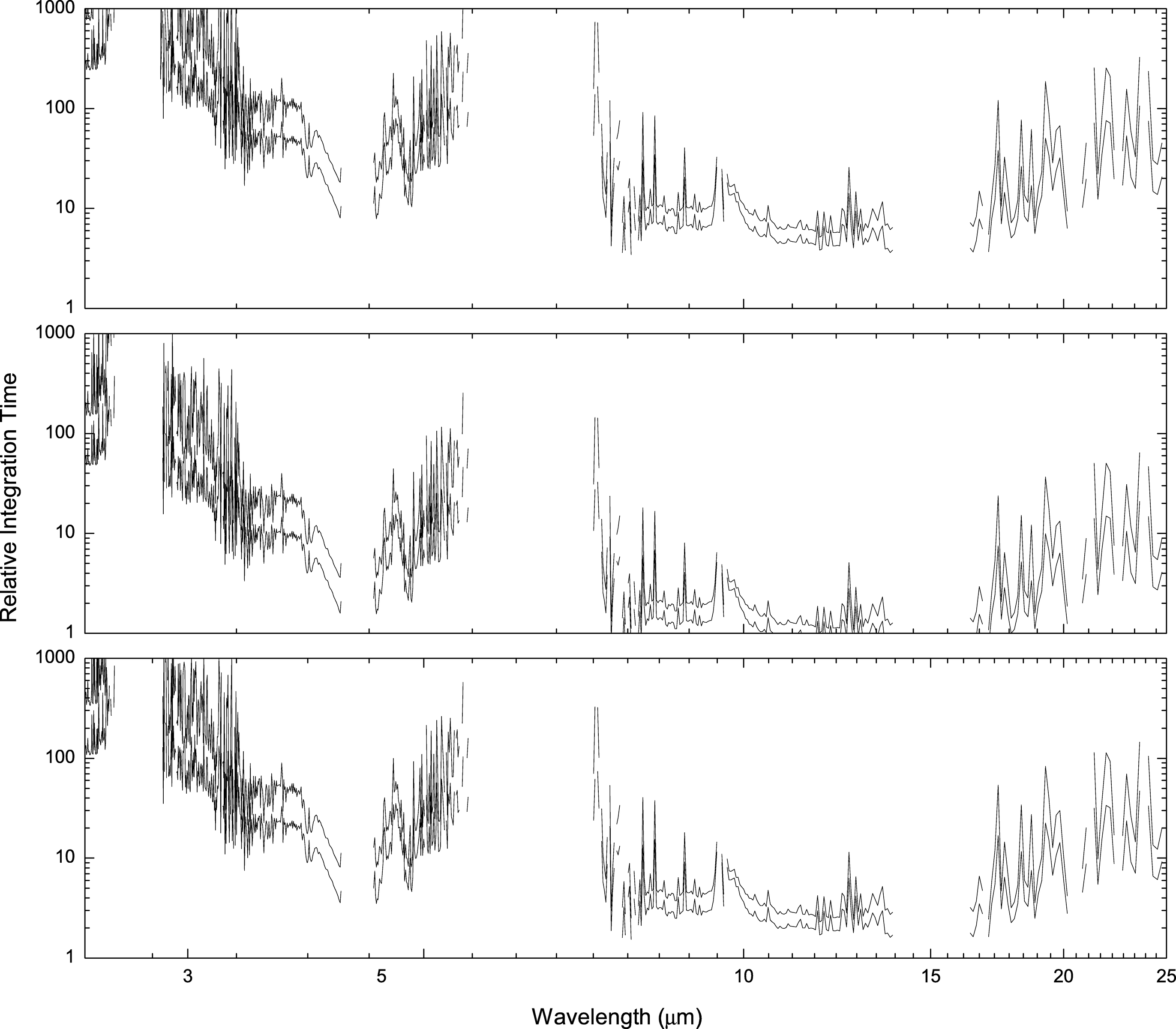
Fig. 9.— Ratio of point‐source integration times for a 30 m Mauna Kea telescope with a 30 m Antarctic telescope (top panel) and a 20 m Antarctic telescope (bottom two panels). Each telescope is seeing limited (with the same seeing size) for the middle panel. Each telescope is diffraction limited in the bottom panel. In each panel, both Dome C (lower curve) and Dome A (upper curve) sites are considered. Values are only shown for wavelengths at which the Mauna Kea transmission is greater than 10%.
The diffraction‐limited condition is not really appropriate for this full range of wavelengths, because of the difficulties in adaptive correction of such large telescopes. The seeing‐limited condition considers that the integrated seeing is the same for each site. The actual sensitivity ratios will lie somewhere between these two cases, depending on the exact site turbulence conditions and the degree of adaptive optics correction. The only available data from Dome C show an average seeing of 1 1 in summer (Aristidi et al. 2003). While it will be some time before wintertime seeing statistics are available from Dome C, there are many reasons to believe the winter seeing is significantly lower than this—primarily because of the lower wintertime temperature inversion layer (Travouillon et al. 2003). In addition, aerological data from the South Pole have shown remarkably low high‐altitude turbulence and wind speed. If the same conditions are observed at Dome C, then adaptive optics correction becomes much more efficient (Lawrence 2004). Hence, the relative sensitivities of Dome C and Dome A telescopes could actually be much better than shown here.
Throughout the wavelength range 30–300 μm, a quantitative comparison of Antarctic sites to even the best ground‐based submillimeter sites (such as Chajnantor Plateau) is meaningless, as the mid‐latitude atmospheric transmission is so low at temperate sites that observations are not possible. This is one of the motivations for developing an airborne observatory. The performance of such observatories, however, is limited by several factors: the turbulence generated by high‐velocity airflow can seriously degrade resolution at shorter wavelengths; scalability to large apertures or interferometers is restricted; and observing time is also limited. Although complete wavelength coverage is not possible from the Antarctic sites, the ability to deploy large apertures is a distinct advantage. Shown in Figure 10 is the relative sensitivity of the 2.4 m SOFIA telescope compared with a 12 m telescope at Dome A and Dome C. In transmissive regions, both Antarctic telescopes are orders of magnitude more sensitive than SOFIA. This wavelength region represents perhaps the greatest opportunity for the development of Antarctic telescopes. As the majority of resources available to space telescopes is currently directed toward coverage of the optical and near‐infrared, the domes of the high Antarctic Plateau represent the only place high spatial resolution observations in the mid‐ and far‐infrared can be performed.
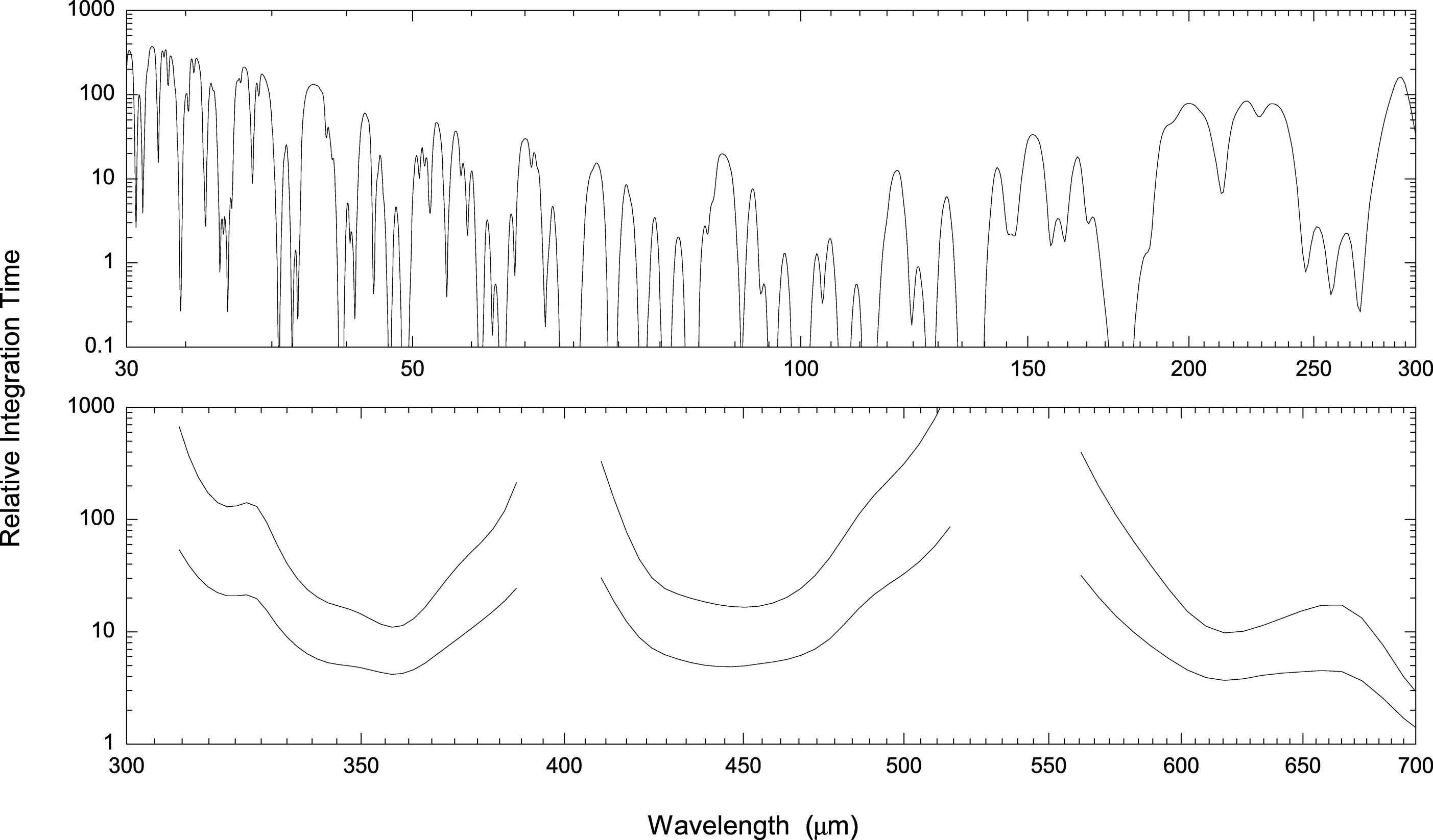
Fig. 10.— Ratio of point‐source integration times for a 2.4 m airborne telescope (top panel) and a 15 m Chajnantor Plateau telescope (bottom panel) to a 12 m Antarctic telescope. In each panel, both Dome C (lower curve) and Dome A (upper curve) sites are considered. Values are only shown for wavelengths at which the Chajnantor Plateau transmission is greater than 10%.
Submillimeter observations longward of about 300 μm become possible in only a few windows from mid‐latitude sites. There are a number of existing and planned single‐dish submillimeter telescopes, such as the 15 m JCMT (Mauna Kea) and the 12 m APEX prototype of ALMA (Chajnantor Plateau). A 12 m Dome C or Dome A single‐dish telescope represents a significant improvement in sensitivity to these telescopes, as shown in Figure 10.
7. CONCLUSION
The highest infrared and submillimeter sensitivity over the largest range of wavelengths can always be achieved through the deployment of space telescopes. The large costs associated with such space missions, however, seriously limit the available aperture, and thus high spatial resolution observations can best be achieved with very large aperture ground‐based telescopes and interferometers. While a large number of parameters are required to fully quantify a particular site, in terms of point‐source sensitivity, the Antarctic Plateau sites examined here have been shown to be unequalled. In addition, significant differences (up to 2 orders of magnitude) are found between the four Antarctic sites. These results exemplify the importance of the continuing site characterization of the high‐plateau sites. It is important to verify experimentally the theoretical predictions presented here of wintertime Dome C sky emission and transmission. In addition, it is also essential to obtain wintertime data on the turbulence profile and seeing statistics from Dome C in order to better gauge the overall site quality. Although it will be some time before the possible development of a station at Dome A, the extraordinary benefits offered by this site justify its consideration in the long term.
The author thanks Von Walden of the University of Idaho for supplying his South Pole LBLRTM models, which have proved extremely helpful. Michael Ashley, Michael Burton, Paolo Calisse, and John Storey of the University of New South Wales Antarctic research group have provided valuable comments regarding this paper, and Christian Meyer has provided a reduction of AWS data. Dome Fuji data from Ebihara Yusuke of the Japanese National Institute of Polar Research, and Vostok data from Valery Lukin of the Russian Antarctic Expedition, is appreciated. This research is funded by the Australian Research Council.
Footnotes
- 1
See the Antarctic Meteorological Research Center archive of Antarctic radiosonde data at ftp://ice.ssec.wisc.edu/pub/southpole/radiosonde.
- 2
See the NOAA Climate Monitoring and Diagnostics Laboratory data archive at http://www.cmdl.noaa.gov/info/ftpdata.html.
- 3
See footnote 1.
- 4
See the Antarctic Meteorological Research Center archive of Antarctic Automatic Weather Station data at http://uwamrc.ssec.wisc.edu/archiveaws.html.
- 5
See footnote 4.
- 6
From the 1977–1999 yearly climatological summary table available from the NOAA Climate Monitoring and Diagnostics Laboratory at http://www.cmdl.noaa.gov/met/.
- 7
See footnote 3.
- 8
See the model Mauna Kea near‐infrared atmospheric emission spectra by Phil Puxley available from the Gemini Web site at http://www.gemini.edu/sciops/ObsProcess.
- 9
See the NASA Infrared Telescope Facility documentation on Mauna Kea sky background measured with the NSFcam instrument at http://irtfweb.ifa.hawaii.edu/Facility/nsfcam/hist.