
ABSTRACT
We describe the design and construction of a formatted fiber field unit, SparsePak, and characterize its optical and astrometric performance. This array is optimized for spectroscopy of low surface brightness extended sources in the visible and near‐infrared. SparsePak contains 82, 4  7 fibers subtending an area of 72'' × 71'' in the telescope focal plane and feeds the WIYN Bench Spectrograph. Together, these instruments are capable of achieving spectral resolutions of λ/Δλ∼20,000 and an area–solid angle product of ∼140 arcsec2 m2 per fiber. Laboratory measurements of SparsePak lead to several important conclusions on the design of fiber termination and cable curvature to minimize focal ratio degradation. SparsePak itself has throughput above 80% redward of 5200 Å and 90%–92% in the red. Fed at f/6.3, the cable delivers an output of 90% encircled energy at nearly f/5.2. This has implications for performance gains if the WIYN Bench Spectrograph were to have a faster collimator. Our approach to integral‐field spectroscopy yields an instrument that is simple and inexpensive to build, yet yields the highest area–solid angle product per spectrum of any system in existence. An Appendix details the fabrication process in sufficient detail for others to repeat. SparsePak was funded by the National Science Foundation and the University of Wisconsin‐Madison Graduate School, and is now publicly available on the WIYN Telescope through the National Optical Astronomical Observatories.
Export citation and abstract BibTeX RIS
1. INTRODUCTION
Observational astronomy consists of obtaining subsets of a fundamental data hypercube of the apparent distribution of photons in angle2 on the sky × wavelength × time × polarization. Information‐gathering systems ("instruments") are designed to make science‐driven trades on the range and sampling of each of these dimensions. Here we describe an instrument optimized for the study of the stellar and ionized gas kinematics in disks of nearby and distant galaxies. Such studies require bidimensional spectroscopy at medium spectral resolution (5000<R<20,000, where R≡λ/Δλ) of extended sources over a relatively narrow range of wavelength (e.g., ∼600 spectral channels) with no consideration of time sampling or polarization.
What is paramount for our application is the ability to gather sufficient signal at low light levels and medium spectral resolution. Etendue (the product of area, solid angle, and system throughput) at constant spectral resolution and sampling is the relevant figure of merit. To characterize the light‐gathering aperture alone, here we also refer to "grasp" (the area × solid angle product).
Field of view and spatial resolution are also of merit, but of secondary importance. For our particular application, we require the number of spatial resolution elements be sufficient to resolve galaxy disks out to 3–4 scale lengths at several points per scale length—about 15 points across a diameter. The matching of overall scale is dictated, then, by the telescope and fiber size needed to reach the required spectral resolution and etendue with an affordable spectrograph. That is, the galaxies are to be chosen to fit the instrument.
Bacon et al. (1995) and Ren & Allington‐Smith (2002) discuss the trade‐offs between spatial and spectral dynamic range and sampling for a variety of spectroscopic instruments—all fundamentally limited by the two‐dimensional sampling geometry of their detector focal planes. An evaluation of this discussion shows that integral‐field spectroscopy (IFS) and Fabry‐Perot (FP) imaging are the preferred methods for bidimensional spectroscopy at low light levels. Each has its merits. Relative to FP imaging systems, IFS systems trade spatial resolution and coverage for spectral resolution and spectral coverage. For emission‐line studies in need of high spatial resolution, FP is optimal. For lower spatial resolution, particularly at high spectral resolution, where the FP "bull's eye" is small, IFS is particularly competitive. (The "bull's eye" is the angular diameter in which the central wavelength shifts by less than the spectral resolution.) For absorption line studies in which many spectral channels are needed, IFS is superior. This condition becomes even more pronounced if spectral resolution and etendue are valued more highly than spatial resolution, as we do here.
Within the realm of "integral field" spectroscopy, there is still a wide range of spatial and spectral sampling (see Ren & Allington‐Smith 2002). Our interest is in fiber‐fed or image‐slicing systems that reformat the telescope focal plane (i.e., into a slit), optimizing for spectral sampling while still retaining bidimensional spatial coverage (cf. SAURON [Bacon et al. 2001a], which is optimized for spatial sampling at the sacrifice of spectral sampling). While image slicers minimize entropy increases, fibers relax the restriction on the spatial sampling. In some situations, the entropy increase (i.e., information loss) from fibers via focal‐ratio degradation (FRD; see Angel et al. 1977; Barden et al. 1981; Clayton 1989; or Carrasco & Parry 1994) may be more than compensated by the increased flexibility in how the fibers sample the telescope focal plane and are mapped into the dispersive optical system.
For example, fibers offer the advantage of formatted sampling in that they intentionally sample not an integral area, but instead some structured, coherent yet dispersed pattern. While this "patterning" has not been used in fixed‐bundle arrays, there are clear advantages to this approach. For an extended object, all spatial elements do not carry equal scientific weight, and there is a trade between coverage and sampling. Fibers allow these trade‐offs to be fine‐tuned. In the specific example of galaxy kinematic studies, one may choose to allocate fibers to sample both major and minor axes, or perhaps uniformly cover a larger physical area with sparse sampling such that lower surface brightness outer regions are still sampled more frequently than the inner, higher surface brightness cores. The latter is the approach we have adopted here.
These considerations led us to our design of a formatted fiber array for the WIYN Bench Spectrograph—the first of its kind. It is a simple, inexpensive instrument providing dramatic gains in information‐gathering power for a broad range of scientific programs that require bidimensional, medium‐resolution spectroscopy at low surface brightness levels. The SparsePak design is in an orthogonal direction to most 8 m class IFU instruments, which strive to maximize spatial resolution at high cost and complexity and at the loss of medium spectral resolution for background‐limited observations.
Our strategy was to take advantage of an existing spectrograph with a very long slit (equivalent to about 12') and capable of echelle resolutions to optimize the study of galaxy kinematics at low surface brightness. The result of this mating of fiber cable to spectrograph yields a bidimensional spectroscopic system capable of achieving spectral resolutions and grasp comparable to the best systems on any telescope. The specific grasp of SparsePak—the grasp per spatial‐resolution element—is the highest of any spectroscopic instrument (see Fig. 1). It is this singular attribute that allows SparsePak to be used effectively at low surface brightness and medium spectral resolutions. This fiber array was completed on 2001 March 10, installed in 2001 May, and successfully commissioned over the following month.
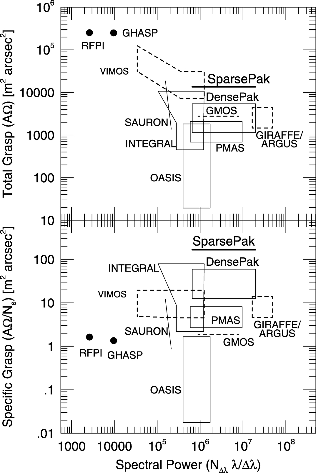
Fig. 1.— Grasp vs. spectral power for a current suite of two‐dimensional spectroscopic systems, including SparsePak (see text). The total grasp is defined as the product of area × solid angle (AΩ). The specific grasp is the grasp per spatial resolution element (in the case of SparsePak, this is per fiber); Ns is the number of spatial resolution elements. The spectral power is defined as the product of the spectral resolution R = λ/Δλ times the number of spectral resolution elements NΔλ. Spectographic instruments on 8 m class telescopes are shown as dashed lines (Gemini/GMOS, VLT/VIMOS, and VLT/ARGUS); spectographic instruments on 4 m class instruments are shown as solid lines (WHT/SAURON and INTEGRAL, CFHT/OASIS, Calar Alto/PMAS, and WIYN/DensePak and SparsePak); Fabry‐Perot instruments (GHASP and RFPI) are shown as filled circles. The variations in the shapes of covered parameter space depends on how a given instrument achieves a range of spectral resolution and spatial sampling (i.e., through changes in gratings, slit widths, or both). Note the unique location of SparsPak in these diagrams.
In a series of two papers we describe the design, construction, and performance of this array and its associated spectrograph. We start in § 2 with a basic description of SparsePak and the spectrograph it feeds, as well as a comparison of SparsePak to existing fiber arrays on WIYN and other telescopes. In § 3 of this paper we present the design goals and constraints that led to the SparsePak formatted‐array design. A synopsis of SparsePak's technical attributes are presented in § 4. The construction of single‐fiber reference cables are also documented. This cable provides a benchmark for evaluating the laboratory‐measured performance of SparsePak. Sections 5 and 6 contain the astrometric and optical properties of the array, as measured in our lab. In § 7 is a summary of our results. An Appendix contains a technical description of the fabrication process in sufficient detail for others to repeat the process.
In Paper II (Bershady et al. 2003) we establish the on‐sky performance of the array and spectrograph in terms of throughput, spectral resolution, and scattered light; we demonstrate the ability to perform precision sky‐subtraction and spectrophotometry; and we present examples of commissioning science data that highlight the capabilities for which SparsePak was designed.
2. BASIC DESCRIPTION
SparsePak is a formatted, fiber‐optic field unit that pipes light from the f/6.3 Nasmyth imaging ("WIYN") port to the WIYN Bench Spectrograph (Barden et al. 1994). The plate scale at this port is 9 374 mm−1. The highly polished SparsePak fibers have no foreoptics nor antireflection coatings. The WIYN port has no corrector nor atmospheric dispersion corrector (ADC). Hence, there are only the three reflective telescope surfaces upstream of the fibers. The cable transmittance was measured in the lab to be near 85% at 6500 Å.
At the WIYN port, each of SparsePak's 82 active fibers has an active diameter of 4 687. SparsePak's grasp is ∼11,200 m2 arcsec2, or 137 m2 arcsec2 per fiber.6 The minimum fiber spacing (center to center) is 5 63, due to buffer and cladding. Figure 2 shows the astrometric format of the array. Active fibers are sparsely placed in a nearly 2' × 2' array of 367 mechanical‐packing fibers. Seventy‐five active fibers form a 720 × 713 sparsely packed grid offset into one corner of the array. This forms the "object" area of the array. Except for a core region, one out of every three fibers in this grid is an active fiber. The core region is densely packed with 17 fibers and has a fill factor of 64.5% within areas defined by seven hexagonally packed, contiguous fibers (equivalent to a filling factor of ∼55% over an angular extent of 39'' × 24''). The overall fill factor of the object area is 25.4%. The final seven active fibers serve to sample the sky. They are well spaced along two adjacent edges of the grid in an L‐shaped pattern, between 61 9 and 85 6 from the central fiber of the grid. There is a ∼25'' gap between the edges of the grid and the sky fibers. These "sky" fibers are uniformly distributed across the fiber slit that feeds the spectrograph.

Fig. 2.— Astrometric diagram of the SparsePak array head at the WIYN Nasmyth imaging port (bare RC focus). Active (science) fibers are numbered according to their position in the slit. The relative size of the fiber core and the core plus buffer is shown to scale for the unnumbered, inactive, or buffer fibers. The active fibers have the same geometry. On‐sky orientation at the WIYN IAS port with zero rotator offset places north upward and east to the left (also as viewed in the WIFOE slit‐viewing camera). Physical measurements were made in our lab (as described in the text); angular dimensions are based on these measurements using the nominal WIYN bare‐RC imaging‐port plate scale of 9 374 mm−1.
2.1. Comparison to DensePak and Other Bidimensional Spectroscopic Instruments
SparsePak complements the existing WIYN/DensePak array (Barden et al. 1998). DensePak has 91 fibers, each 2 81 in diameter, arranged in a 7 × 13 rectangular (but hexagonally packed) array. DensePak fibers are spaced at 3 75 center to center, such that the array has the approximate dimensions of 27'' × 42'' on the sky at the f/6.3 Nasmyth port. While SparsePak has coarser and sparser sampling relative to DensePak, SparsePak has a factor of 3 larger grasp and roughly 5 times the sampled angular footprint.
SparsePak's enhanced grasp makes it well suited to studies of extended sources at low surface brightness, particularly because SparsePak is capable of spectral resolutions that are comparable to those obtained with DensePak. This is made possible by using spectrograph settings at which the anamorphic demagnification is large (see § 2.2 below, and Paper II). It is these very configurations that yield the medium spectral resolutions (5000–25,000) that we desire for galaxy kinematic studies. At these resolutions, sources with narrow emission lines can even be studied in bright time in the red, with a minimum penalty payed for higher continuum background. However, the key gain of SparsePak over DensePak is the ability to stay background‐limited at these medium spectral resolutions in reasonable exposure times.
Figure 1 illustrates the grasp versus the spectral power for a representative sample of current, bidimensional spectroscopic systems. The spectral power is the product of the spectral resolution and the number of spectral resolution elements sampled by the spectrograph. Spectrographic instruments on 8 m class telescopes include Gemini's GMOS (Allington‐Smith et al. 2002), the Very Large Telescope's VIMOS (Le Fèvre et al. 2003) and GIRAFFE/ARGUS (Pasquini et al. 2002). Spectrographic instruments on 4 m class telescopes include the William Herschel Telescope's SAURON (Bacon et al. 2001a) and INTEGRAL (Arribas et al. 1998), the Canada‐France‐Hawaii Telescope's OASIS (Bacon et al. 2001b), Calar Alto's PMAS (Kelz et al. 2003), and WIYN's DensePak and SparsePak. Interferometric instruments include the Rutgers Fabry‐Perot Interferometer (RFPI), used on the CTIO 1.5 and 4 m telescopes (Schommer et al. 1993; Weiner et al. 2001), and GHASP (Garrido et al. 2002), used on the Observatoire de Haute‐Provence 1.93 m telescope. Figure 1 shows the wide range in trade‐offs made by instruments in terms of spatial and spectral information collection, as discussed in § 1.
SparsePak falls in a unique location in the parameter space of Figure 1, having both one of the larger total grasps and spectral power and the highest specific grasp of any instrument. This superior performance comes at a cost, namely in spatial resolution. In contrast, 4 m class instruments such as SAURON and OASIS are optimized for higher angular resolution. This too comes at a cost. These instruments sacrifice being able to achieve higher spectral resolution for sky‐limited observations. Even instruments on 8 m class telescopes are unable to achieve the specific grasp of SparsePak. This places SparsePak in a position to achieve the highest possible spectral resolutions for sky‐limited observations.
2.2. The Bench Spectrograph
The Bench Spectrograph is a bench‐mounted, fiber‐fed spectrograph situated in a climate‐controlled room two stories below the telescope observing floor. The spectrograph can be optimized for a wide range of gratings, because of its adjustable camera collimator and grating angles, and adjustable grating camera distance.
The existing grating suite includes six low‐order gratings with rulings between 316 and 1200 and that are blazed between 4° and 31°, and an R2 echelle (316 lines mm−1 blazed at 63  4). These are used respectively at nominal camera collimator angles of 30° and 11°. Although this angle is adjustable, in practice this option has not been exercised. The echelle grating delivers between 2 and 5 times higher spectral resolution than the low‐order gratings, while the latter deliver greater efficiency and increased spectral range at the cost of resolution. Consequently, the delivered product of spectral resolution × slit width, Rφ, and throughput have a wide range of values. This is quantified in Paper II.
There are two features of note concerning the Bench grating suite relevant to SparsePak's intended science mission. First, there are large anamorphic factors for the echelle and low‐order gratings blazed above 25°, such as the 860 line mm−1 grating. With the echelle grating, the anamorphic demagnification is significant such that with even the 500 μm SparsePak fibers, the delivered instrumental spectral resolution R is ∼10,000, with the FWHM sampled by 3.5 pixels. This is equivalent to a velocity resolution of 12.7 km s−1 (σ).
Second, the echelle grating is used in single‐order mode (i.e., there is no cross‐dispersion). Orders are selected via rectangular narrowband interference filters placed directly in front of the fiber feed. These filters have efficiencies of 90% redward of 600 nm, 80% around 500 nm, and dropping to 60% only as blue as 375 nm. In the red these values are considerably higher than what is achieved with reflection gratings, and hence, for limited wavelength coverage in the red, the Bench has the potential to outperform grating–cross‐dispersed echelles.
Despite this potential, the Bench Spectrograph total system throughput (atmosphere, telescopes, fibers, spectrograph optics, and CCD) is estimated to peak at 5% when using the multiobject fiber feeds (Hydra Users Manual;7 S. Barden & T. Armandroff, NOAO). This value should apply to DensePak as well. Measurements show SparsePak's peak is 40% higher, or roughly 7% (see Paper II). A significant portion of this gain is from decreased vignetting in the fiber "toes" due to our redesign, as discussed in § 4.4. The mean throughput, averaged over all fibers and wavelengths within the field, is significantly lower, and closer to 4% with SparsePak and 2.5% with the Hydra and DensePak cables (see Paper II). The lower mean values are due to the strong spatial and spectral vignetting, which are severe for lack of proper pupil placement. When using the echelle grating, the large (∼1 m) distance between camera and grating required to avoid vignetting the on‐axis collimated beam incident on the grating results in off‐axis vignetting that is is particularly large. In this mode, both spatial and spectral vignetting functions contribute about a factor of 2 at the edge of the field such that the slit ends at the end of the spectral range are down by typically factors of 4 from the peak. We have taken this limitation into account when mapping fibers from the telescope focal plane onto the slit (§ 3.2.6).
It is worth noting why the spectrograph has such severe vignetting. In addition to the lack of pupil reimaging, the spectrograph was designed for a f/6.7 input beam and a 152 mm collimated beam over a modest field. As we show below, the output from the fibers fed by the telescope at f/6.3 are beams with focal ratios between 4.3 and 5.9 at 90% encircled energy (EE). This results in collimated beams of 170–234 mm at 90% EE. While the optics are nearly sufficient for the on‐axis fiber,8 the slit subtends a 4 2 field on the parabolic collimator; the fast‐output beams lead to losses in the system for the off‐axis fibers, compounded by the lack of a properly placed pupil. Because the fiber feed is in the beam, even the on‐axis fibers suffer some (∼9%) vignetting. As we show in Paper II, these geometric considerations allow us to accurately model the observed system vignetting. While the problem is currently severe, our clear understanding of the problem gives good reason to believe that significant improvements in the spectrograph optical system can be made in the near future.
2.3. Efficacy
Given the Bench Spectrograph's low throughput, would a higher throughput, long‐slit system be more competitive than SparsePak? The long slit, for example, would be stepped across a source in repeated exposures. There are three primary reasons why SparsePak will far outperform a long‐slit spectrograph:
- 1.The equivalent number of long slits is ∼15, requiring a throughput of the combined spectrograph, telescope, and atmosphere of 105%! This is a factor of 3–5 times higher than what can be accomplished with the best contemporary systems. While the improved filling factor of stepped long‐slit observations is equivalent to 3 SparsePak pointings (see § 5), truly integral‐field spectroscopy is not needed for all applications. Hence, only in the most extreme scenario (in which integral‐field spectroscopy is needed and a long‐slit system has 35% efficiency) will long‐slit observations break even in terms of efficiency.
- 2.The long‐slit observations would not be simultaneous, and hence conditions may vary, leading to uncertainties in creating spectrophotometric maps.
- 3.The astrometric registration of stepped long‐slit observations would be less certain.
Finally, as a general statement of cost‐effectiveness, it should be cheaper to build or upgrade a wide‐field, high‐resolution spectrograph that is bench‐mounted and fiber‐fed rather than a direct‐imaging system attached to a telescope port.
3. DESIGN
3.1. Science Drivers
Our aim is to provide a survey engine capable of measuring nearby spiral galaxy kinematics over most of the optical disk for the purpose of determining their dynamics and their luminous (stellar) and dark content. Since the distribution of mass can only be directly measured by dynamical means, spatially resolved galaxy kinematics provide direct constraints on the origin and evolution of disk galaxies.
In order to study the large‐scale dynamics of the optical disks of galaxies, the disks must be spatially well sampled, with spectroscopic measurements out to several scale lengths Rs. These measurements must be at sufficient spectral resolution and signal‐to‐noise (S/N) to determine both precise rotation and nonaxisymmetric bulk motions, as well as velocity dispersions in both gas and stars. In addition to spatial and spectral sampling and coverage, further technical requirements include minimizing systematic errors due to cross talk and sky subtraction. We discuss these science‐driven technical requirements in turn.
3.1.1. Spatial Resolution and Sampling
Consider first the spatial resolution and sampling requirements. Typical disks have exponential scale lengths of 2–5 kpc in size. To be well sampled, there should be 2–3 to three measurements per disk scale length. In the inner regions, where the rotation curve rises and changes shape rapidly, the sampling should be finer by additional factors of 2–3. In the outer regions, where the disk is fainter, it is important to have more solid angle sampled, such that the limitations of decreased surface brightness can be overcome by co‐adding signal (e.g., within annular bins). A generic, scale‐free requirement, therefore, is for enhanced resolution at small radii, and enhanced coverage (solid angle) at large radii. The latter is naturally achieved by a two‐dimensional sampling pattern.
The absolute spatial scale is set by disk‐galaxy structure that, if not fully understood from a theoretical perspective, is at least observationally well defined. Two to three disk scale lengths represents a threshold for the mass distribution within spiral galaxies in terms of transitions between different components of the overall mass distribution. At these distances, rotation curves are expected to be flat, or at least to have transitioned from the steep, inner rotation curve rise to a more shallow rise or fall. Hence, with rotation curves extending out to these radii, one may suitably estimate a terminal rotation velocity and total dynamical mass. Since the disk is expected to contribute maximally to the overall enclosed mass budget near 2.2 Rs (Sackett 1997), dynamical disk‐mass estimates need to probe out to at least these distances.
For a finite number of fibers of a fixed physical size on a given telescope, the above requirements imply a sampling area, resolution, and pattern that is highly specific for galaxies of a particular angular size. The only way to substantially increase the dynamic range in this case is to modulate the input plate scale via foreoptics (which may include lenslets). Such optics introduce additional light losses both from reflections and, in the case of lenslets, from misalignment or nontelecentricity (Ren & Allington‐Smith 2002). Plate‐scale modulation is limited by the numerical aperture of the fibers (roughly f/1.3–f/2 at the coarse limit) and by the need to feed the fibers at a sufficiently fast f‐ratio to avoid introducing significant FRD (roughly f/4–f/6 at the fine limit). At fine plate scales, the grasp is decreased, and consequently so too is the achievable depth. Alternatively, for a given spectrograph, one may choose the largest possible fibers that maximize the grasp in the absence of foreoptics while yielding the required spectral resolution. Targets can then be chosen to suit the above sampling criteria. Since galaxies are found in a wide range of apparent sizes, we chose this latter path.
For a fixed‐scale integral field unit (IFU), it is still possible to fine‐tune the spatial sampling geometry to allow for some dynamic range in spatial scale. Indeed, there is recourse in carefully designing a sampling pattern to be coupled with specific observational techniques (i.e., dithering patterns). Herein lies a critical advantage of fibers for formatted patterns, or what we call "formatted field units" (FFU). In other words, since fibers are convenient light pipes, it is not necessary to sample truly integral regions of the sky, but instead one can consider optimal geometries to accomplish a specific science goal.
Our original pattern consisted of four rotated long slits (at position angles of 0°, ±30°, and 90°) and an integral inner region (Bershady 1997; Bershady et al. 1998; Andersen & Bershady 1999). However, these designs required rotation to fill in interstitial regions and did not provide more sampling of a solid angle at larger radii. Ultimately, the FFU concept led us to develop a pattern with wide areal coverage with sparse sampling in a rectangular grid, combined with a densely sampled core, as per the above desiderata. The pattern described in § 2 allows for simple dithering either to fill the sparsely sampled grid or to critically subsample the core, as discussed in § 5. The rectangular grid is also convenient for tiling of very large sources. Further, a rectilinear sampling provides a variety of radial samplings when centered on an axisymmetric source. The final pattern is well suited to the study of normal, luminous spiral galaxies with recession velocities of (roughly) 2000–10,000 km s−1.
3.1.2. Spectral Resolution
The second consideration is the spectral resolution required to measure disk kinematics. While disks have typical rotation velocities of the order of 100 km s−1, the nonaxisymmetric motions are of the order of 10 km s−1, as too are the velocity dispersions in both gas and stars. In particular, the vertical component of the stellar velocity ellipsoid σz is expected to be of the order of ∼10 km s−1 for the outer parts of disks, based on what we know of disk stars in the solar neighborhood and from long‐slit measurements of a handful of nearby galaxies (Bottema 1997). In order to optimize the measurement of σz in galaxies of known rotation velocity, nearly face‐on galaxies must be targeted. This optimizes the projection of σz, but minimizes the projection of the rotation velocity. This is a reasonable trade, since the rotation velocity is typically an order of magnitude larger than the velocity dispersion.
While it is possible to centroid a high‐S/N line to better than 10 times the instrumental resolution, the same precision cannot be achieved (at a given S/N) for the higher order moments of line width (σ), skew, and kurtosis (the latter two are equivalent to the Gauss‐Hermite polynomial h3 and h4 terms). Intuitively, one can understand that higher order profile information requires better resolution or better S/N. Consequently, the desired precision of the velocity dispersion measurements provides the driver for the required spectral resolution.
To reliably measure velocity dispersions of 10 km s−1, we estimate that instrumental resolutions of ∼10,000 are necessary. This statement is qualified by the obtainable S/N. A full treatment of the trade‐offs of profile‐moment precision versus S/N is beyond the scope of this work. However, we find that S/N of 15–20 in a spectral line yields line‐width measurements at a precision of 10% for widths at the instrumental resolution. Given the trade‐offs between grasp and spectral resolution (larger fibers collect more light but yield lower spectral resolution), we estimate that absorption‐line S/N of greater than 20–30 is unlikely to be obtained in the outer parts of disks for any reasonable exposure times on 4 m class telescopes. Consequently, it is not possible to push too far below the instrumental resolution for any reasonable precision. Hence, for stellar velocity dispersions studies in dynamically cold disks, adequate spectral resolution is at a comparable premium to S/N and spatial resolution.
3.2. Practical Constraints
The design of SparsePak is constrained by mating to an existing telescope feed and spectrograph. For practical purposes, we accepted the limitations imposed by this existing hardware. Our adopted fabrication process also imposed certain practicalities. We mention here those constraints that are relevant to placing limits on our science goals.
3.2.1. Fiber Size
Based on our experience with fibers, we find that 500 μm is a maximum practical thickness for the active diameter so that the fiber stiffness does not cause frequent breakage in handing. Fortuitously, this corresponds to the maximum size we would want to consider, based on our interest in achieving spectral resolutions of an order of 10,000 using the echelle grating with the Bench Spectrograph.
3.2.2. Spectral Coverage
Because SparsePak is built for an existing spectrograph, spectral coverage is not a design issue per se. However, we did consider whether the Bench Spectrograph's spectral coverage was suitable for our science goals. Given the large suite of gratings, a wide variety of spectral coverage is available. For kinematic studies, however, we are interested in the higher dispersion gratings. What is relevant, really, is the number of independent‐resolution elements NΔλ, which, depending on the setup (i.e., the degree of demagnification) is between 600 and 800. In general for spectral resolutions R, the spectrograph will cover a spectral range of NΔλλ/R. For R = 10,000, the covered range is several hundred angstroms in the optical. This is sufficient to cover the Mg i region from [O iii] λ5007 past the Mg i b triplet and [N i] λ5200 stellar absorption lines; or the Hα region from [N ii] λ6548 to [S ii] λ6731; or all three lines of the Ca ii near‐infrared triplet at λλ8498, 8542, and 8662.
Greater spectral coverage is generally advantageous for cross‐correlation work in weak‐line regions, such as the Mg i region near λ5130, since the desired power in the cross‐correlation comes from many weak (e.g., Fe i) lines spanning a wide range of wavelengths. For a finite detector focal plane, increased spectral coverage comes at the cost of decreased spectral resolution or spatial coverage. The optimum trade is highly dependent on the scientific goals, but it is unlikely that the current system is far off for studies of stellar kinematics in galaxies.
3.2.3. Cross Talk
Integral‐field spectroscopy is likely to have cross talk between individual spatial channels in the telescope focal plane, due to the blurring effects of the atmospheric point‐spread function. While there is no indication of fiber‐to‐fiber cross talk for the types of fibers we have used (i.e., photons do not leak out of the fiber cladding and penetrate the cladding of a neighboring fiber), for fiber‐based integral‐field units, there is an added consideration.
Because of the azimuthal scrambling in fibers and the requisite remapping of the two‐dimensional telescope focal plane into the one‐dimensional spectrograph slit, nonadjacent fibers in the telescope focal plane will be adjacent in the slit. This can lead to spatially incoherent but systematic cross talk. To minimize systematic effects, it is therefore desirable to adequately separate fibers along the slit. The specific fiber separation depends on the optical quality of the spectrograph optics (both aberrations and scattering), as well as the scientific need to control the level of systematics.
For SparsePak, given the large fiber buffers (0 9 edge to edge for the most closely packed fibers) and excellent WIYN image quality (a median seeing of 0 8 FWHM), there is very little coupling between fibers in the telescope focal plane. Hence, the only significant cross talk would take place at the spectrograph slit. Because of the difficulty in assessing the effects of systematic errors due to cross talk, we have chosen conservative limits. Our adopted science requirement is to limit cross talk to under 1% for discrete spectral features from adjacent fiber channels. This limits systematic effects to 10% for adjacent fibers with factors of 10 differences in signal flux. Such variations in signal are likely worse‐case, given the fiber mapping and the astrophysical variations of, e.g., Hα emission within galaxy disks. Incoherent cross talk (i.e., scattering into and out of the source spectrum) limits are below 10%, with a goal of under 1%. This component mainly affects the delivered S/N in an rms sense. Because incoherent scattering takes place over larger physical scales, it is dominated by the spectrograph optics. Fiber separation (§ 3.2.4) is designed, then, to meet the requirement for coherent scattering even when on‐chip binning by factor of 2 in the spatial dimension. (On‐chip binning is important for low light level applications and provides significant gains, given the large projected fiber diameter onto the CCD—roughly 4 unbinned pixels in the spatial dimension.)
3.2.4. Total Fiber Number
At the spectrograph input focal plane, the maximum slit length currently used by any of the fiber feeds9 is 76.4 mm.
There is also a minimum fiber‐to‐fiber separation at the spectrograph feed to prevent significant cross talk between fibers. This is a function of the scattering properties and image quality of the spectrograph. To meet the design requirements of § 3.2.3, we estimated that ∼400 μm was the minimum acceptable edge‐to‐edge distance between the active regions of fibers at the spectrograph slit. This estimation was based on the performance of three existing fiber feeds for the WIYN Bench Spectrograph. A detailed measurement of the SparsePak cross talk is presented in § 5 of Paper II.
The above combination of maximum slit length, minimum fiber separation at the slit, and maximum fiber size constrains the total number of fibers and hence the overall maximum grasp of the system. A maximum of 82 fibers with 500 μm diameter cores was chosen. These fibers map into a 73.6 mm slit. An additional two to three fibers could be added to bring the slit length up to the nominal 76.4 mm value of the other Bench cables. However, due to the strong vignetting within the spectrograph, the addition of extra fibers offered little gain.
3.2.5. Array Size
At the telescope focal plane, we are limited by the existing telescope‐mounting hardware. The entire fiber array assembly (array plus its mount) must fit within a cylindrical mount with a 1 inch (25.4 mm) outer diameter. The array had to be rectangular in cross section, given the way in which it was glued (as described in § A.5). This yields a maximum array dimension (cross section) not to exceed ∼12 mm, which corresponds to a maximum field of view of 112'' (diameter), with diagonals up to 160''.
This limiting field of view of the FFU is comparable to the size of nearby normal luminous spiral galaxies. To maximize the distance between the object grid and the sky fibers, the object grid is placed in one corner of the fiber array, and the sky fibers are then placed in an L‐shaped pattern around the two far sides (see Fig. 2).
3.2.6. Minimizing the Effects of Vignetting
The mapping of fibers between telescope and spectrograph input focal planes is complicated, because of several redesigns of the active fiber layout during construction. However, one of the goals was to put some of the fibers in the center of the source grid near the outside of the spectrograph slit, and vice versa, the reason being that since astronomical sources are generally centrally concentrated, this would balance the strong vignetting in the spectrograph. Ideally, we would have adopted a more ordered mapping (e.g., Garcia et al. 1994), but the large fiber diameter and fiber‐to‐fiber separation makes the details of the mapping largely unimportant.
3.3. Sky Subtraction
Random and systematic errors in sky subtraction have plagued fiber‐fed spectroscopic measurements. Here we explain our fiber allocation, which is calculated to minimize random errors, and discuss how careful placement and treatment of sky fibers in the spectrograph and telescope focal planes help limit systematic errors.
3.3.1. Optimum Number of Sky Fibers
Wyse & Gilmore (1992) calculate the optimum allocation of fibers to source and sky for the particular case of random errors in which source flux and sky flux are equal. Here we consider a similar calculation, but for the two extreme cases of background‐ and detector‐limited observations. These are more relevant for observations at low surface brightness and high spectral resolution.10
The adopted merit function assumes one is trying to achieve a specified S/N for a given number of sources (Nsource) in the least amount of total observing time (ttotal). (Here S/N can be defined as any linear function of the S/N per recorded detector element.) Observation of these Nsource sources constitute a "survey." In other words, one would like to maximize the merit function fmerit = Nsource/ttotal. Further, we assume that a spectrograph is fed by a finite number of fibers (nf) that can be used for any given observation; that some number (ns) of these fibers will be used for sky; that a survey may consist of more than one observing set (e.g., Ntotal>nf - ns); and that sky can be subtracted perfectly—in a statistical sense, i.e., sky contributes to shot noise, but not to systematic error.
In the background‐ and detector‐limited regimes,
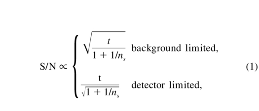
where t is the observing time for a given source, which can be expressed as

These equations can be combined to solve for the survey merit function
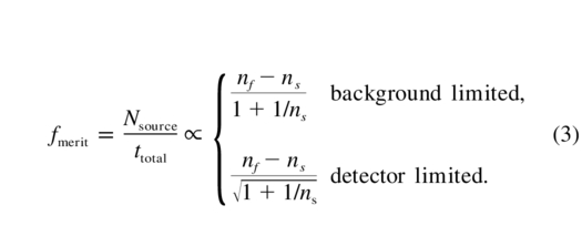
Maximizing the merit function with respect to ns (at fixed S/N and nf) yields quadratic relations with these exact solutions:
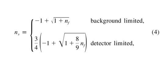
which are plotted in Figure 3.
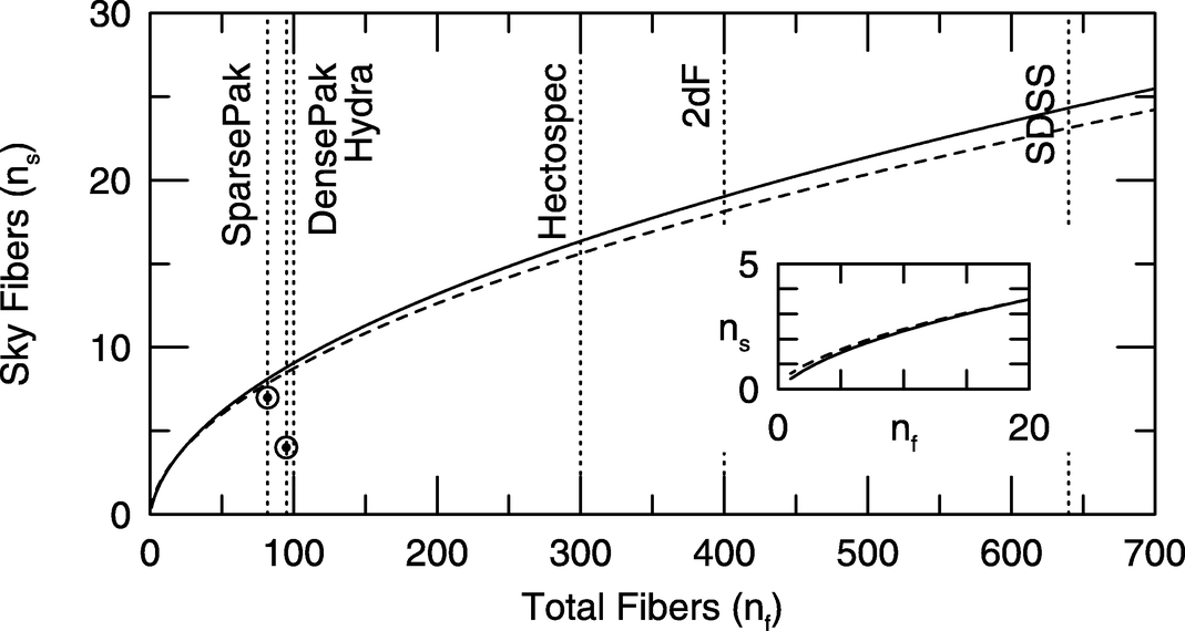
Fig. 3.— Optimum number of fibers dedicated to sky (ns) plotted as a function of the total number of spectrograph fibers (nf). This assumes that sky backgrounds and their subtraction contribute only to random (shot) noise (i.e., systematic errors are not considered in this model). Background‐limited measurements are indicated by the solid line; detector‐limited measurements by the dashed line. An insert illustrates the behavior at small nf. The two points represent the number of sky fibers allocated for SparsePak and DensePak. For SparsePak, the optimum number of sky fibers is ∼8, while for DensePak the optimum number is 9; the allocated numbers are 7 and 4, respectively. However, the survey merit function defined in the text is a weak function of ns. The relevant number of sky fibers for several other survey spectrographs are indicated.
Equation (4) is a general result for background‐ and detector‐limited surveys, which are essentially identical. This result is independent of spectral resolution and of whether source fibers target many individual targets or are bundled into a single IFU targeting one extended source. Examination of Figure 3 indicates that SparsePak, with 82 total fibers, should have on the order of 8 sky fibers. For reasons of symmetry in the object grid, we chose to allocate seven. In contrast, DensePak has four allocated sky fibers, whereas the optimum number is closer to nine. So while it may appear that DensePak is more efficient by allocating fewer fibers to sky, from a survey perspective SparsePak is closer to the ideal. However, the merit function is not strongly dependent on the number of sky fibers. The value of the merit function for DensePak, for example, is only 6% lower than its optimum value.
3.3.2. Slit Mapping
Our argument in the previous section does not take into account instrumental issues that affect the final data quality and the ability to extract signal accurately. While scattered light plays an important role in the ability to accurately subtract background continuum, the primary contribution to systematic errors in the subtraction of spectrally unresolved sky lines are the field‐dependent optical aberrations present in spectrographs (Barden et al. 1993b). The WIYN Bench Spectrograph, for instance, uses a parabolic collimator with field angles ranging from 0° to 2 1. Evidence for field‐dependent effects are shown by Barden et al. (1993a) for the Mayall 4 m Ritchey-Chrétien (RC) spectrograph, and also in the Two‐Degree Field (2dF) system as reported by Watson et al. (1998): with sky fibers concentrated in one area of of the slit, sky residuals increase for fibers farther away along the slit.
One technique for dealing with the issue of aberrations is known as "nod and shuffle" (Glazebrook & Bland‐Hawthorn 2001), whereby the telescope is nodded between source(s) and sky at the same time that the charge is shuffled accordingly on the detector. While initially presented in the context of multislit spectroscopy, nod‐and‐shuffle can be applied to multifiber spectroscopy as well. This technique has the advantage of putting both sky and source flux down the same optical path, while sampling both over the same period of time. The more traditional "beam switching" technique (e.g., Barden et al. 1993b), for example, suffers from an inability to sample source and sky at the same time. However, both techniques suffer from allocating 50% of the observing time to sky. This is equivalent to allocating half of the total fibers to sky. While nod‐and‐shuffle undoubtedly achieves the smallest level of systematic error, the penalty in terms of the above survey merit function (random error) may be too high. An alternative approach may be to try and map the optical aberrations within the spectrograph system (e.g., Viton & Milliard 2003).
For our purposes, implementing nod‐and‐shuffle is beyond the scope of the current effort. We have chosen instead to carefully place our seven sky fibers such that they sample at nearly uniform intervals along the slit. With the reasonable assumption that the optical aberrations are symmetric about the optical axis, we expect to be able to model the aberrations empirically via these small number of sky fibers. The success of this method, and its dependence on any differential FRD within the fibers, is demonstrated in Paper II. At present, what is relevant for the instrument design is the concept of mapping the sky fibers in the focal plane across the slit.
3.3.3. Sky Fiber Placement within the Fiber Array
Our experience with DensePak (Andersen 2001) indicates that the DensePak sky fibers behaved differently from those sampling the source. In this FFU, the "source" fibers are glued together coherently into a rectangular array, while the sky fibers are separately mounted in hypodermic needles and are offset from the array. The differences we found were such that the continuum levels measured in the sky fibers were systematically above or below the continuum in the "source" fibers after field flattening, even when the array was pointed at blank sky. While we never determined the exact cause of this systematic behavior, it seemed reasonable to suppose that differences in fiber termination may have played a role. For this reason, we designed SparsePak to include the sky fibers within the same coherent fiber bundle as the source fibers.
3.4. Summary of Design Considerations
The final SparsePak design was dictated by a confluence of and compromise between scientific objectives, technical performance goals, and mechanical and fabrication constraints. Within the confines of the existing spectrograph and telescope feed, the spatial and spectral sampling were the key drivers that determined the fiber size and layout of the SparsePak FFU. Cross talk was a secondary condition that provided some limits on the fiber packing and hence the total number of fibers. Sky subtraction dictated some additional fine‐tuning of the fiber allocation and placement. The above discussion provides generic requirements for yielding adequate observational data for a wide range of dynamical studies in the context of the practical constraints of the WIYN telescope feed and existing Bench Spectrograph.
4. TECHNICAL SYNOPSIS
Summarized here are the technical attributes of the SparsePak cable detailed in the Appendix and deemed directly relevant to its performance.
4.1. Head Construction: Buffering
The fiber head has short "packing" fibers surrounding the long, active fibers cut from the same Polymicro batch. These serve as mechanical elements and provide an edge buffer with a minimum thickness of one fiber. The buffer is intended to minimize stress on the active fibers and maximize their condition uniformity. The success of this buffer arrangement is evaluated in § 6.
4.2. Cable Design
The cable consists of an outer sheath of heavy‐gauge flexible stainless‐steel conduit and an inner PVC tube jointed every 6 feet to provide natural spacing within the larger steel conduit. Within the PVC cable run 82 black Teflon tubes (each containing one fiber). The stainless‐steel flex conduit serves to protect against fiber crushing and overbending. The PVC and Teflon provide safe, smooth inner surfaces for the Teflon and fiber, respectively. We believe this design is successful in minimizing stress‐induced FRD along the cable length, although the addition of thermal breaks in the Teflon would be advantageous in future designs (Fabricant et al. 1998).
4.3. Cable Termination and Interfaces
The cable is terminated with mounts whose design is dictated to a large extent by existing mounting hardware in the telescope and spectrograph focal surfaces. Three significant modifications were made within these constraints. (1) To ensure and maintain telecentricity of fibers in the telescope focal plane, the head‐mount dimensions were precisely machined, and a support brace attaching to WIFOE (a mounting box named after the WIYN Fiber‐Optic Echelle) was made. (2) An antirotation collar was placed roughly 250 mm back from the end of the fiber head to prevent the bare fibers from twisting. (3) The mount to the spectrograph has a modified slit block, and the exit aperture of the filter‐holding "toes" has been enlarged considerably. The latter allows up to an f/4 unvignetted beam to exit the fibers into the spectrograph. Measurements presented in Paper II show that this enlargement may increase the throughput by ∼20%.
One last feature of the existing mounting hardware to note here is the fiber foot (where the cable terminates for mounting on the spectrograph). As we evaluate in § 6, this curvature is too sharp and is the principal cause of FRD in the system.
4.4. Reference Cables
To determine the effects of the cable manufacturing process that are specific to the FFUs on fiber throughput and FRD, and to provide a stable reference for future testing, we produced several single‐fiber "reference" cables. Two of these cables were made from the 500 μm fiber: a "short" cable 1.5 m length, and a "long" cable 24.5 m in length. The last meter of each cable is covered with the identical black, opaque Teflon used in the FFU cables. The remainder of the fiber is uniformly coiled on the initial foam packing spools on which the fiber came. The fiber ends all terminate inside microtubes of appropriate diameter and are glued with a single drop of Norland 68 UV curing epoxy. These tubes are themselves glued into machined brass ferrules suitable for mounting on an optical bench with standard hardware or into our circular‐lap polisher. The fiber‐polishing process is identical to that used for the FFU cables on this polisher. As expected, no hand‐polishing was necessary.
These reference cables represent an idealized application of astronomical fiber light conduits in that they have excellent polish, the glue type is superior, the glued surface area is minimal, and there is otherwise little stress (or change in stress) on the optical fibers.
5. ASTROMETRIC SPECIFICATIONS
Final SparsePak head dimensions were measured in our lab independently by two skilled technicians, each using two different micrometer engines. The final SparsePak array of 23 × 20 fibers is very close to 12.05 mm2 at the front face. This maps to 113 0 at the WIYN imaging port (IAS), assuming the nominal plate scale of 9 374 mm−1. The precise dimensions are 12.09 ± 0.05 mm in width and 12.01 ± 0.03 mm in height, as detailed in Figure 2.11 The array is square to within 0.6% ± 0.3%. The array dimensions imply average fiber‐to‐fiber separation at the face, in width and height, of 525.6 and 600.5 μm, or 4 927 and 5 629, respectively. The array dimensions also imply an average glue thickness of 0.5 μm where the fiber buffers abut. Measurements of the array dimensions along the 50.8 mm length of the glued volume indicate a flaring of − 013 ± 001 in width and +010 ± 007 in height, where the sign of the flaring indicates whether the flaring is toward (+) or away (−) from the central axis of the fiber head. The amplitude of this bundle flaring is well under our tolerance limit in terms of the FRD error budget: differential effects, center to edge, are well under 0 1.
Astrometry based on direct imaging of the fiber face (e.g., Fig. 11) indicates that the fiber‐to‐fiber spacing is uniform within our measurement errors (1% of fiber width, or <0 05). A table of astrometric positions of the fibers relative to the central fiber (No. 52), which is useful for creating maps of extended sources, is available at the SparsePak Web site.12 Two common observing offset patterns are also provided there. The "array fill" pattern of three positions provides complete sampling at every fiber position (e.g., every 5 6) within the nominally sparsely sampled 72'' × 71'' grid. This pattern is useful, for example, for creating velocity fields of spiral disks (e.g., Andersen & Bershady 2003; Courteau et al. 2003; Swaters et al. 2003). The "array subsample" provides critical sampling; i.e., at every half‐fiber position in both dimensions (roughly 2 8 spacing) within the densely sampled core. This pattern is useful for obtaining the highest spatial resolutions within the inner 39'' × 25'' region of an extended object. By combining these two patterns (nine positions total), critical sampling is achieved over the full 72'' × 71'' grid.
6. OPTICAL PERFORMANCE
Prior to shipping and installing the SparsePak cable onto WIYN, we characterized the completed cable on an optical test bench in our lab. The test bench system was designed to measure absolute throughput and FRD at a number of optical wavelengths for which we had available filters.
6.1. Optical Test Bench
The test bench setup, illustrated schematically in Figure 4, consists of a double‐reimaging system using commercially available 2 element, 50 mm achromats. The concept is based on earlier systems developed by S. Barden and L. Ramsey, as reported by Ramsey (1988): a differential flux and flux‐profile comparator is made from two optical reimaging systems with an intermediate focus that can be switched between (1) a "straight through" mode in which the first reimaging system directly feeds the second, and (2) a "fiber" mode in which the first reimaging system feeds a fiber that then feeds the second reimaging system. Modes 1 and 2 differ only by the presence of the optical fiber inserted at the intermediate focus, which forms an optical diversion adding zero net length to the imaging portion of the system. The modes are selected by the simple translation of a precision stage that holds the entire first reimaging system and the output end of the fiber.
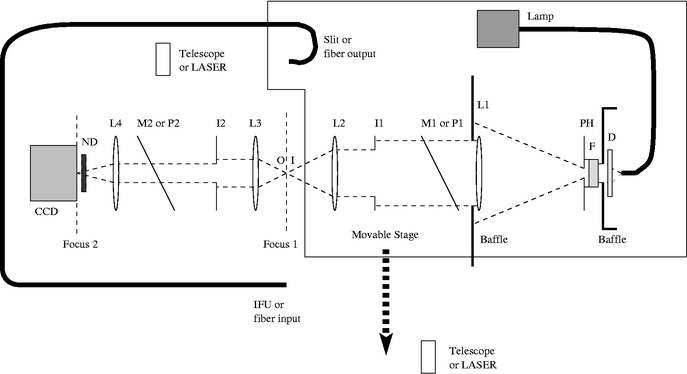
Fig. 4.— Schematic diagram of our test bench for characterizing the throughput and FRD of the optical fibers. The setup consists of a double‐reimaging system. The first system (right side, moving left from lamp through camera optic L2), is on a translation stage such that it can either feed the second system directly or via a fiber feed. The setup is illustrated for the direct feed, or "beam mode." The "fiber mode" is accomplished by moving the translation stage such that the input (I) of Focus 1 from the first system is placed on the fiber input or IFU (refer to labeled points). This translation also moves the fiber output or slit into the former position of Focus 1 to create the output (O) that feeds the second system (refer to labeled points). The second system (left side, moving left from collimator optical L3 to the CCD detector) is fixed. Mirrors and pellicles (P1/M1 and P2/M2) are placed into the collimated beams for alignment purposes. Irises (I1 and I2) are for controlling the input and output f‐ratio, respectively. Details of the light source, diffuser (D), filter (F), and pinhole (PH) setup, as well as the CCD and neutral‐density filters (ND), are given in the text.
The first reimager places an image of a uniformly illuminated pinhole at an intermediate focus with a beam of known and modulatable f‐ratio (the "input f‐ratio"). As noted above, this focus can be transferred either directly to the second reimaging system ("beam mode") or into a fiber ("fiber mode"). In fiber mode, the fiber feeds the second reimaging system. In both cases, the second reimaging system transfers the intermediate focus to the surface of a CompuScope CCD.13 This detector has a 768 × 512 format of 9 μm2 pixels. The second reimaging system has a known and modulatable "output f‐ratio."
For both reimaging systems, the f‐ratio modulation is accomplished with a graded iris placed in their respective collimated beams. Ideally, the iris would be placed at the pupil formed by the collimator lens, but space limitations on our optical bench prevented us from doing this. Given the small field used in the system (i.e., the image is a pinhole), the vignetting produced by our setup is negligible. Because the camera lenses are oversized, given the effective beam stops of the irises, it is unnecessary for the camera optics to be at the collimator pupil. Pellicles were inserted into the collimated beams of both reimagers for initial optical alignment (by visual inspection via a telescope, and by tracing via a laser feed). One pellicle was used during the measurement stage in the first reimaging system for alignment of the intermediate focus onto the fiber.
Pinholes were illuminated by a lamp via a coherent fiber bundle illuminating a baffled diffuser and then a filter, in that order. We found that this specific setup and careful baffling of the pinhole illumination was essential to minimize scattered light. Because of their small size, filters were placed between the baffled diffuser and the pinhole. Neutral density (ND) filters were also required, since high lamp intensities were needed for source stability and optical alignment, and to place the pinhole image on the fiber face. Placement of the NDs in front of the CCD considerably eased the measurement process.
The size of the pinhole is dictated by the magnification of the first reimaging system and the desire to under‐ or overfill the fiber face. For the test bench measurements reported here, we used lenses with 250, 200, 150, and 100 mm focal lengths at L1 through L4, respectively. We chose a 400 μm pinhole for SparsePak such that the reimaged size at the intermediate focus was 320 μm. As such, this permitted us to illuminate a large fraction of the fiber face while being sure that all of the incident flux went into the fiber. We also tried a smaller, 10 μm pinhole to verify that (1) all of the light was being fed into the fiber, and (2) that FRD measurements did not depend on the specific input modes filled at a constant f‐ratio. For example, with the smaller pinhole, we were able to align the spot on the middle and edge of the incident fiber face. The results of these tests with the smaller pinhole were positive, so we focus below on results using the 400 μm pinhole.
The filters available at the time of SparsePak testing consisted of a "standard" UBVRI set. Narrower bandwidths are desirable, particularly in the blue, where fiber and CCD response change rapidly with wavelength.
6.1.1. Comparison to Other FRD Measuring Engines
The difference between our experimental design and earlier ones (e.g., Ramsey 1988) is in the details of the optical arrangement, optomechanics of the alignment process, and the use here of an areal detector instead of an aperture photometer. The use of a CCD reduces sensitivity to defocus, permits a better understanding of optical alignment and focus, and yields more accurate and precise estimations of the total transmitted light (via the ability to perform multiaperture photometry and determine background levels).
However, we have not taken full advantage of the areal detector, namely to image the far‐field output pattern of the direct and fiber‐fed beams. This would directly allow us to measure the effects of FRD on the beam profile in one step; i.e., we wouldn't need measurements at multiple f‐stops, as described in the § 6.2. Carrasco & Parry (1994) have effectively implemented such a scheme by placing the CCD camera directly behind what would be our first focus. The disadvantage of their scheme is that a precisely repeatable back focal distance must be ensured, since they are imaging an expanding beam.
A viable alternative for future consideration is to place the CCD at the pupil of what is our second collimated beam. In practice this requires the necessary optics to make a small enough collimated beam to match the available CCD, and possibly the addition of a field lens near the first focus (our Focus 1) to place the pupil at a back distance convenient for CCD mounting.
A system such as we have just described can be competitive with and certainly complementary to the "collimated beam" approach described by Carrasco & Parry (1994). The latter uses a laser to directly probe the FRD at a given input incidence angle and then relies on a model to synthesize the full effects of FRD on an astronomical beam profile (i.e., a filled cone with obstructions). The approach described here is model independent, provides a means for also measuring total throughput, and may provide a simpler and more cost‐effective way to measure the wavelength dependence of throughput and FRD.
6.2. Laboratory Measurements
For each filter and fiber, the idealized measurement process consisted of (1) establishing the optical alignment of the system at a given input f‐ratio; (2) obtaining a measurement of the beam‐mode flux at an output f‐ratio of f/3 ("open"); (3) transferring the setup to fiber mode and carefully aligning the pinhole image with the fiber center; (4) obtaining a series of fiber‐mode flux measurements while varying the output f‐ratio from f/3 to f/12 (typically 5–10 exposures at a given f‐ratio); (5) reacquiring beam mode and taking an identical series of flux measurements. Postacquisition image processing was done via IRAF, the goal of which was simply to measure a total flux from the pinhole or fiber‐output image incident on the CCD.
Considerable care was taken with mounting SparsePak and the reference cable to ensure that the fibers were aligned to the optical axis within 0 2. As with telescope alignment, even small off‐axis angles induce appreciable FRD. In the case of SparsePak, the mounting hardware was considerable, given the bulk and stiffness of the cable and the need to actuate the slit between fiber and beam modes.
Due to the short time period between completing SparsePak's manufacture, the final alignment of the test bench, and the shipping date, characterization of the SparsePak fibers were done within the short period of 6 days between 2001 April 19 and 24. Some of these measurements are known to have been problematic in terms of optical alignment. We were careful to note when we thought the placement of the pinhole image on the fiber was poor or uncertain, or if other aspects of the optical setup were questionable. With the exception of lamp variability (which might produce errors of either sign), all of the other systematics in our measurement process would lead to underestimating the true throughput of the fibers. As we will show, the measurements we were able to obtain give consistent and plausible results that show that SparsePak is a high‐throughput fiber cable with explainable trends in FRD.
6.3. Fiber Transmission
We have measured the total fiber transmission for 13 SparsePak fibers in the B, V, R, and I bands for an input f‐ratio of 6.3. We have also made identical measurements for the SparsePak reference fiber, both at f/6.3 and f/13.5 input focal ratios. The SparsePak fibers were chosen to lie over a range of positions within the SparsePak head, and to span the slit. The total fiber transmission is defined to be the light transmitted within an output beam of f/3. As we show in § 6.4, the encircled energy as a function of output f‐ratio converges by this value.
Recall that fiber throughput measurements are done in a differential way by comparing the total counts measured with the test bench CCD in "imaging" and "fiber" modes. What we report, then, is a measurement of the total fiber transmission, which includes end‐losses. As noted, measurement systematics that we could identify included lamp drift or poor alignment of the illuminated, reimaged pinhole onto the fiber. For the latter we had to rely on detailed measurement log notes. For the former, we could check the stability of the observed flux over a series of measurements at a fixed iris aperture, as well as compare initial and final beam‐mode fluxes. Of the 13 fibers measured, 5 were flagged as being problematic: No. 37, 39, 72, 81, and 82.
The results of our measurements are presented in Figure 5. The eight fibers for which we have robust measurements in all bands are in agreement with expected values based on the manufacturer's attenuation specifications plus two air‐silica interfaces—at least at wavelengths corresponding to V, R, and I bands. In the B band our measurements appear too high. This is because we have not correctly assessed the color terms of the bandpass and hence the proper effective wavelength for the measurements. We estimate that the combination of the relatively cool lamp filament (due to modest lamp intensity to optimize stability), red fiber transmission, and dropping quantum efficiency of the detector in the blue yields an effective wavelength closer to 4900 Å for the B filter. From inspection of Figure 5, one can see that our measurements through the B filter are in agreement with the predicted performance, assuming such a red effective wavelength.
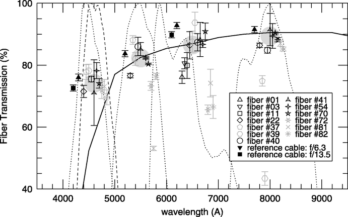
Fig. 5.— Fiber transmission (throughput) of 13 of the 82 SparsePak fibers and the SparsePak reference cable, measured using the test bench in our lab, as described in the text and illustrated in Fig. 4. Symbols denote different fibers, as identified in the key, and are offset in wavelength within groups for presentation purposes. Light symbols (gray instead of black) are fibers for which the throughput variance across bands was larger than 15%. These fibers either had measurement log notes indicating unsatisfactory setup of the pinhole image on the fiber face, or beam‐mode measurement variances indicating the lamp stability was poor. As such, these measurements should be viewed as suspect, consistent with the unusually high or low measured transmittance. The large gray circles are the median of the eight good fiber measurements. The solid curve is the expected transmittance of 25.4 m of Polymicro ultralow OH‐ fused‐silica fiber, based on Polymicro's figures, combined with two silica‐air interfaces (3.43% per interface). The dotted curves represent the normalized broadband filter transmission, convolved with the CCD response function. Left to right: B, V, R, and I. For V, R, and I, note the excellent agreement between the measured and expected values, which is the measurable difference between different fibers. The B‐band measurements appear high relative to expectations. The dashed curve takes into account the effective bandpass given the expected fiber transmittance. Not taken into account is the spectrum of the light source. The likely effective wavelength of the B‐band measurements is 4900 Å.
Finally, we found that the reference cable had systematically higher transmission than the median value for the SparsePak fibers—roughly 3%–4%. One might be tempted to conclude that this is an FRD‐related effect (see below). However, in no case does the reference cable have higher transmission than the best‐transmission measurement for the SparsePak fibers. Moreover, the transmission appears to be somewhat lower (3%) for the reference cable fed at f/13.5 instead of f/6.3. We conclude that transmission variations between reference and SparsePak fibers is not significant.
In summary, the SparsePak fibers are red‐optimized and deliver total throughput consistent with manufacturer's specifications. The total throughput rises above 80% redward of 5000 Å, reaches 90% redward of 6500 Å, and peaks near 92% at 8000 Å.
6.4. Focal Ratio Degradation
While the total transmission of SparsePak fibers is high, also relevant to spectrograph performance is the effective output focal ratio of the fibers. A telescope delivers a converging (conical) fiber‐input beam with a constant surface brightness cross section and square edges in the far field for a point source. Telescope obstructions (e.g., secondary and tertiary mirrors) make the beam profile annular, still with constant surface brightness within the far‐field annulus. The effect of fiber microfractures or microbends (see, e.g., Carrasco & Parry 1994) scatters or redirects the incident light such that the output focal ratio is faster and the beam profile softer (a beam cross section no longer has constant surface brightness, and the edges are soft even in the far field). This is FRD.
Fibers thus degrade the input beam by radial scrambling and hence increase entropy (they also provide complete azimuthal scrambling, but this is unimportant here). The information lost can only be recovered at additional cost (e.g., larger optics at the output end of the fiber). One measure of this signal degradation is to measure the output focal ratio containing some fixed fraction of the total transmitted flux (i.e., the encircled energy). A perusal of the literature (e.g., Barden et al. 1981) indicates that the specific choice of fiducial flux fraction is arbitrary. Carrasco & Parry (1994) prefer to parametrize fiber FRD by a more fundamental parameter that characterizes their adopted microbending model. To the extent that the model is correct, this has the strong advantage of being much more general by enabling measurements of a given fiber to be used to characterize the FRD performance of similar fibers of different lengths. Here we measure the full input and output beam profile, from which any index may be extracted.
In our test bench, we used f/4.5, f/6.3, and f/13.5 beams for the intermediate focus, which feeds the fibers in "fiber" mode. These focal ratios are the input beams produced respectively by the Hobby‐Eberly Telescope (HET) spherical aberration corrector (which feeds the fiber instrument feed), the WIYN Nasmyth imaging port, and the WIYN modified Cassegrain port. We did not simulate, however, any of the central obstructions in these systems. Central obstructions will steepen profiles of EE versus f‐ratio for a pure imaging system. For example, on WIYN the central obstruction is 17.1%, which is equivalent to f/15.3 relative to the f/6.3 beam at the Nasmyth focus; no light is contained in the far field within input cones slower than f/15.3. The effects of FRD will be to scatter light into this slow cone, and also into a cone faster than f/6.3. However, since we are interested primarily in the effect at a small f‐ratio, the effects of the central obstruction will only be important if the radial scrambling is gross. This is not the case. Here we report the results for the f/6.3 beam with the SparsePak and reference fibers.
Figure 6 shows that the SparsePak fibers have a wide range of output beam profiles when all are fed with the same (f/6.3) input beam. As a check on the quality of the imaging system, we also measured the beam profile of the "straight through" system. We find the latter profile is close to the ideal case of a constant surface brightness (perfect) beam, except near f/6.3, where there is a little droop indicating some softness in our profile edges. However, the SparsePak fiber output beams are so substantially aberrated in comparison with the "straight through" beam that the imperfections in the optical system are second‐order effects. What is significant to note is that the reference cable has an output beam profile very similar to the "straight through" system; i.e., the FRD in the reference cable is very low. For example, the reference cable output beam contains over 90% of its signal within f/6.3 (the input f‐ratio), whereas the mean SparsePak fiber contains only 67% of its signal within this same f‐ratio.
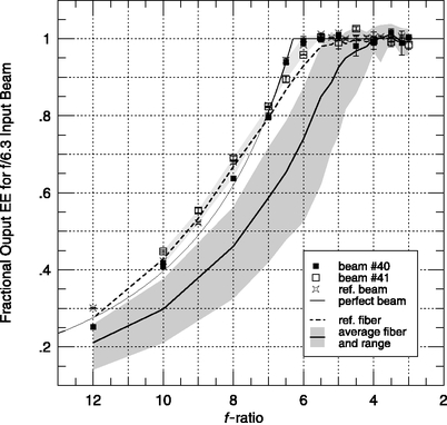
Fig. 6.— Fractional EE as a function of output f‐ratio for an f/6.3 input beam into SparsePak and reference cable fibers. A perfect beam (with constant cross‐sectional surface brightness) is represented by the thin solid line. Straight‐through beam profiles (no fiber) measured when testing three of the fibers (No. 40, 41, and the reference cable) are shown to illustrate the quality of the optical test‐bench setup. The average of the output beam profiles of the fibers is represented by the thick solid line; the gray shaded area represents the range for the 13 SparsePak fibers measured. The range of FRD is real and represents systematic fiber‐to‐fiber differences because of variations in physical conditions of the fibers (see text). The reference cable fiber output profile is the dashed curve. Reducing the curvature of the SparsePak spectrograph feed would dramatically improve the SparsePak fiber profiles.
6.4.1. Wavelength Dependence
We have checked that there is no significant wavelength dependence associated with FRD. Figure 7 shows measurements of output EE at f/6.3 as a function of wavelength between 470 and 800 nm for four representative SparsePak fibers. The variation between fibers at a given wavelength is due to other effects, which we address in § 6.5.
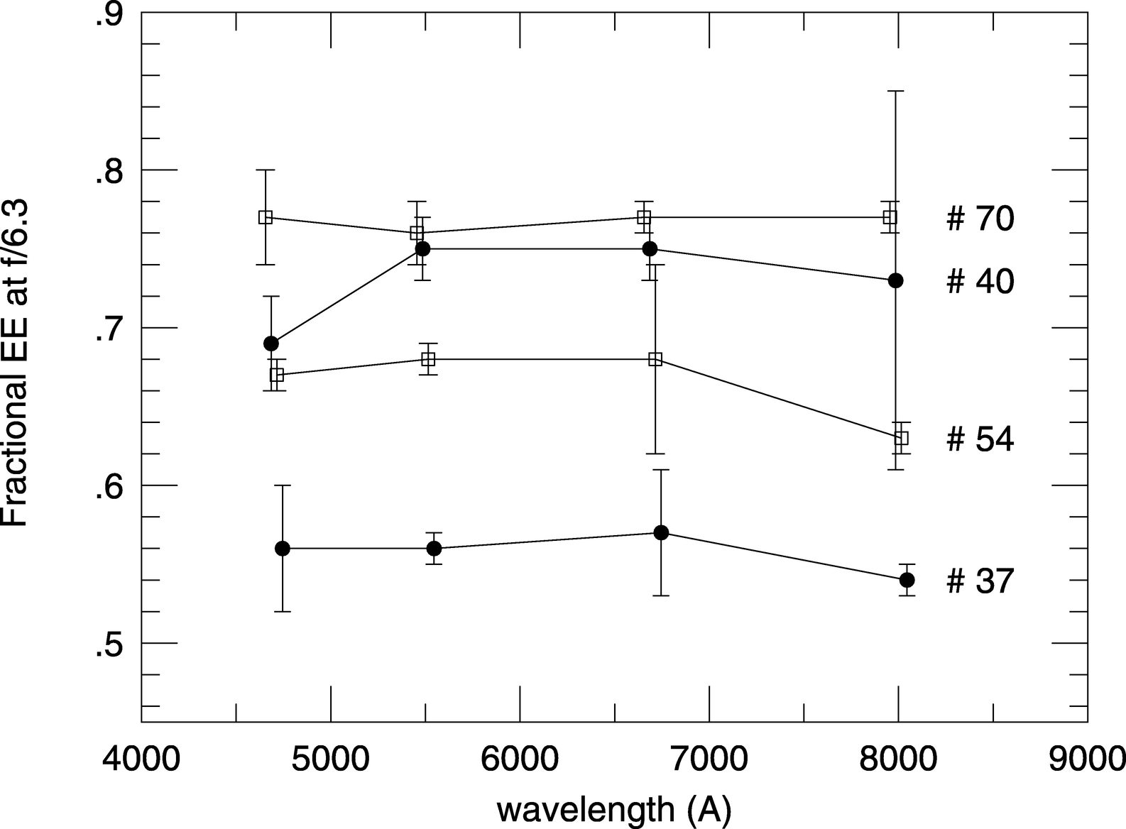
Fig. 7.— Fractional EE at an output f‐ratio of f/6.3 as a function of wavelength for four of the SparsePak fibers (labeled) fed with a f/6.3 input beam. These represent four different measures of FRD wavelength dependence for the 500 μm core Polymicro ultralow OH− fibers. Error bars represent estimated observational uncertainties. Wavelength offsets of points are for presentation purposes.
There is some evidence for a modest FRD increase in the red for the two fibers with the largest FRD, but no evidence for this effect for the fiber with the smallest FRD. This is qualitatively consistent with the microbend model adopted by Carrasco & Parry (1994), which predicts that the broadening width of a collimated beam at large incidence angles is proportional to λ (e.g., a factor of 1.7 between 470 and 800 nm). The effect should become larger when the overall amplitude of the FRD increases. A quantitative test of the wavelength dependence of their model requires more precise measurements, and is worthy of future pursuit; Carrasco & Parry's (1994) direct measurements of the broadening width was a factor of 2 short of the model predictions. Other work by Schmoll et al. (2003) indicates that there is little wavelength dependence to FRD, and cite other theoretical work that predicts that there should be no wavelength dependence. Clearly this issue is not resolved. For our purposes, FRD wavelength dependence, if real, amounts to less than or of an order of a few percent variation in the indices we discuss next.
6.5. Implications for Future Cable and Spectrograph Design
We explored possible causes of the wide range in FRD for the SparsePak fibers seen in Figures 6 and 7. The two likely causes, we believed, would be slit position (due to the systematically changing radius of curvature of the fibers along the slit) and array position, due, possibly, to edge effects. Figures 8 and 9 show, respectively, the f‐ratio at fixed EE and relative EE at a fixed f‐ratio as a function of fiber position along the slit. These figures indeed demonstrate that these two fiber attributes explain essentially all of the profile variance for the SparsePak fibers.
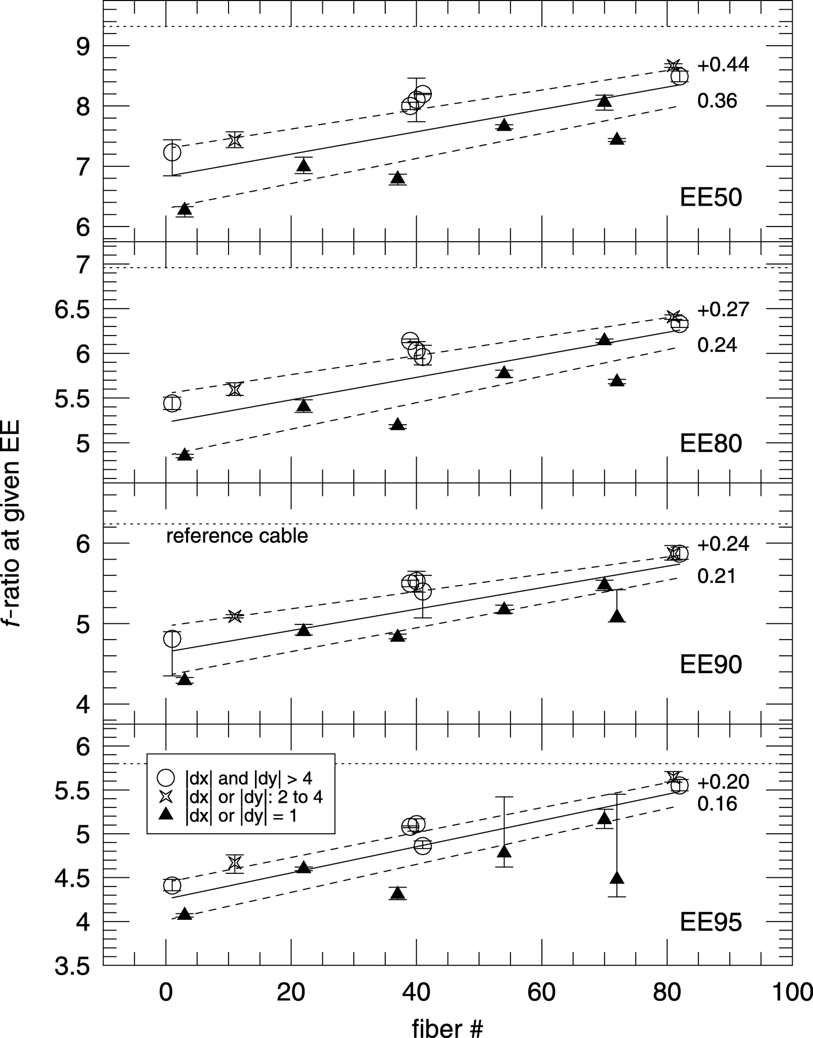
Fig. 8.— Trends of output f‐ratio for four given EE as a function of fiber number and position in the SparsePak array for 13 of SparsePak's fibers (where, e.g., EE50 is 50% encircled energy). All fibers are fed with an f/6.3 input beam. The fiber number, from 1 to 82, corresponds to a fiber's position in the slit and fiber foot. Fiber 1 is on the inside edge of the foot, where the radius of curvature is smallest. Fibers within one fiber diameter of the array edge are marked as solid triangles; fibers within 2–4 fiber diameters of the array edge are marked as four‐pointed stars; all other (interior) fibers are marked as open circles. (No fibers are on the edge, since there is a one‐fiber buffer.) Note the strong, first‐order trend in increased FRD (smaller f‐ratio at fixed EE) with decreasing fiber number (foot radius), and the second‐order trend with distance from the edge of the fiber array. Solid lines are the weighted least squares (WLS) regressions (Akritas & Bershady 1996) to all data. Lower and upper dashed lines are regressions to the outer (|dx| = 1) and inner (|dx|≥2) fibers, respectively; their offset from the solid line at fiber 42 is labeled. The f‐ratio value for the reference cable is marked as a horizontal dashed line. SparsePak fibers approach this limit when they are least bent and more than 2 fibers from the edge of the array. Substantial gains could be had by proper termination of the fiber array cable, most particularly at the spectrograph end (i.e., by straightening the foot).
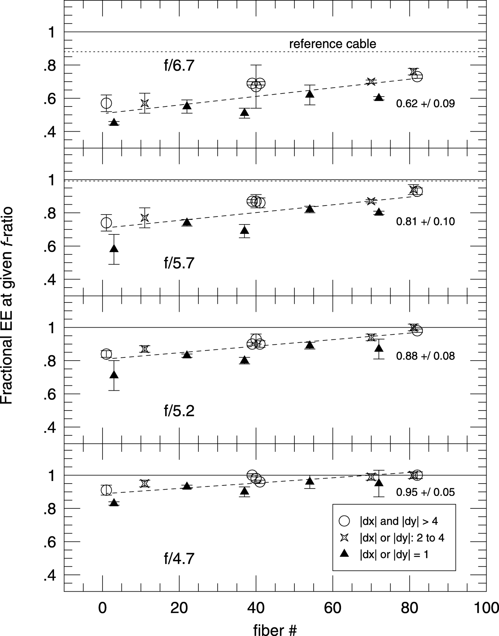
Fig. 9.— Trends of fractional EE vs. fiber number for four output f‐ratios: 6.7, 5.7, 5.2, and 4.7. Symbols are as in Fig. 8 and key. Dashed lines are WLS regressions to all data (Akritas & Bershady 1996) and are labeled for the mean fiber output EE for SparsePak. The dotted line represents the output EE for the reference cable. The solid line at unity is for reference. The Bench Spectrograph optics is designed for a 152 mm collimated beam, which is achieved with the current collimator in an f/6.7 beam. Hence, in the current configuration this beam only contains between 45% and 75% of the light (62% on average).
The first‐order effect is slit position: FRD is greatest for fibers with the lowest numbers, which are at the "top" of the slit, where the curvature in the foot is greatest. The radius of curvature of the fibers goes from 82.6 mm (for fiber No. 1 at the top of the slit) to 178 mm (for fiber No. 82 at the bottom of the slit). We conclude that there would be substantial improvement (a decrease!) in the FRD if the fiber foot were straightened somewhat. The amount of straightening needed is probably slight, given the observed fact that the bottom (least bent) fibers have FRD properties that nearly converge with the reference fiber. Based on extrapolating the trend of EE50 (50% encircled energy) with radius of curvature for the SparsePak fibers to the reference cable, we would recommend a minimum radius of curvature of 240 mm for 500 μm fibers. It is not known if these FRD effects are present for the WIYN cables; these have smaller fibers, which are more flexible. Verification will await on‐telescope measurements of these thinner fibers.
It also appears that fibers within one fiber of the edge of the array suffer a second‐order increase in FRD relative to fibers at comparable slit position but more centrally located within the fiber head. As we discuss in the Appendix, the process of releasing the head from the mold undoubtedly induces stress on the edge fibers. For this reason we introduced a single layer of short packing fibers around the entire array. Clearly, one layer was not enough. However, as seen in Figures 8 and 9, there is no evidence that fibers within two to four fibers' depth from the edge of the array behave any differently than more centrally located fibers. We surmise, therefore, that just one more layer (two layers total) of edge (buffer) fibers would have been sufficient to have prevented this second‐order enhancement of the FRD. We note that we have not proven that the added stress originates from the mold‐release phase. The increased FRD could also stem from the asymmetric distribution of pressure introduced from curing (contracting) epoxy for edge fibers, or from the head‐mount clamp. Whatever the cause, we suspect that this is a generic result, independent of fiber diameter for FFUs manufactured with a similar glue and press. To be safe, we would recommend a minimum of two fiber layers of 500 μm fibers, or the corresponding number of fibers of different diameter to make at least a 1.2 mm buffer.
These results have ramifications for the throughput of the Bench Spectrograph and its improvement, as illustrated in Figures 9 and 10. Currently, an f/6.3 beam is input to the fibers and is then matched to a spectrograph designed for a 152 mm collimated beam. The initial design for the 4 m Mayall telescope had 152 and 203 mm f/6.7 collimators (Barden et al. 1993a). The current Bench on WIYN has a 235 mm clear‐aperture diameter parabolic collimator with a focal length of 1021 mm. This collimator captures an f/4.2 for an on‐axis fiber, but produces a collimated beam substantially in excess of 152 mm. The effective f/6.7 beam is collimated into 152 mm, but contains significantly less than the full output of the fibers.
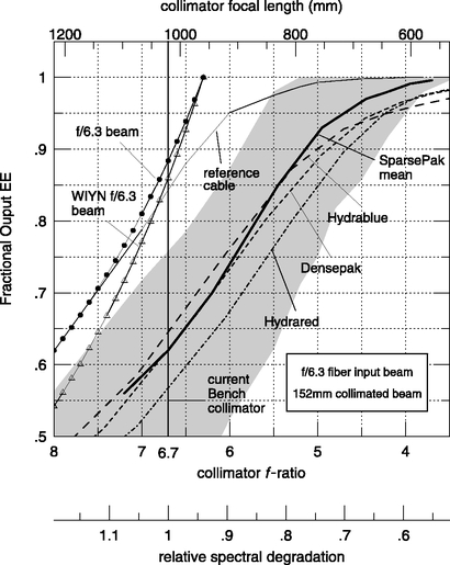
Fig. 10.— Fractional output EE from fibers as a function of WIYN Bench Spectrograph collimator focal ratio (bottom axis) or collimator focal length (top axis). This assumes a 152 mm collimated beam diameter and that all fibers are fed with a f/6.3 beam. The mean SparsePak beam profile (thick solid line), the range for the 13 measured SparsePak fibers (gray shaded area), and reference cable (thin solid curve) are based on laboratory measurements (see Fig. 6) using the f/6.3 input beam shown as a thin solid curve with solid circles. Comparable curves, as measured on the telescope for DensePak (300 μm fibers), and the two Hydra cables (with "blue" 310 μm and "red" 200 μm fibers), are shown for comparison (P. Smith & C. Conselice 1998, private communication; see text for further details). These measurements use the WIYN f/6.3 beam (accounting for the central obstruction; see text), shown as the thin solid curve with open triangles. The very bottom scale (relative spectral degradation) indicates how the spectral resolution of the Bench would alter (worst case) as a result of changes in system demagnification as a function of changes in the collimator focal length at a fixed camera focal length. The current Bench has a f/6.7 collimator for a 152 mm collimated beam. This figure illustrates the effects of FRD on light losses for the Bench Spectrograph, and how optimization trades might be made between throughput and spectral resolution for a redesign of the Bench Spectrograph collimator.
Adopting the mean curve for the laboratory FRD measurements for the SparsePak cable, an f/6.7 beam contains only roughly 62% of the fiber output. The amount of light outside of the 152 mm diameter beam in the current system is in the range of 25%–55%, and 38% on average. (Other curves for DensePak and Hydra cables, measured on the telescope, indicate similar performance [P. Smith & C. Conselice 1998, private communication].) If a faster collimator were used, the fraction of enclosed light in a 152 mm collimated beam would rise to 81%, 88%, and 95% for 870, 790, and 715 mm focal lengths, respectively. With no change in the camera, the resulting spectral resolution will decrease with the increase in the magnification with the collimator focal length. This penalty assumes that the slit is resolved. For smaller fibers and setups with large anamorphic factors, the degradation in spectral resolution will be smaller.
Hence, a trivial upgrade to the Bench Spectrograph, consisting of inserting a faster, parabolic collimator will improve the throughput by 31%, 42%, and 53%, with a loss in spectral resolution less than 18%, 29%, and 42%, respectively, for replacement collimator focal lengths of 870, 790, and 715 mm. The decrease in spectral resolution will be less severe for the smaller fiber diameters, since the current system is undersampled. Based on these results, we argue that a collimator with a focal length near 750 mm would substantially improve the throughput of the spectrograph for acceptable losses in spectral resolution. For some applications, however, the loss in resolution will be unacceptable. One of the better features of the Bench is its modular and accessible design. This means that one could switch with relative ease between one of several collimators.
7. SUMMARY AND DISCUSSION
In this paper we have presented the design, construction, and laboratory measurements of the SparsePak FFU, a formatted fiber‐optic array designed to mate the Nasmyth imaging port to the Bench Spectrograph on the WIYN 3.5 m telescope. A physical description of the SparsePak array is found in §§ 2 and 4, with a complete description of the design and assembly contained in the Appendix. The latter is included specifically to allow others to repeat this relatively simple instrument‐building process.
The primary scientific motivation for this array is to measure the kinematics of stars and gas in nearby galaxy disks. Examples of science capabilities are found in Paper II and in several recent studies using SparsePak to measure stellar velocity dispersions to estimate dynamical mass and the radial dependence of the mass‐to‐light ratio on spiral disks radius (Bershady et al. 2002; Verheijen et al. 2003), the Tully‐Fisher relation in barred spirals (Courteau et al. 2003), and rotation curves and ionized gas kinematics in low surface brightness galaxies (Swaters et al. 2003).
Here we have focused on the confluence of science objectives with the technical, observational, and physical constraints that shaped the specific SparsePak design. The salient design drivers are the balancing of trade‐offs in spatial and spectral coverage and resolution, plus an optimization for superior sky subtraction. For this latter purpose we have developed an analytic expression for the optimum number of sky fibers in the background‐ and detector‐limited regimes. Placement of sky and source fibers along the spectrograph slit are also important considerations in our design, both for sky subtraction and to offset the effects of vignetting within the spectrograph. In Paper II we explore the sky‐subtraction performance of our design. The results presented here and in Paper II are applicable to other fiber‐fed spectrographs.
The SparsePak performance can be summarized in terms of its instrumental grasp of 137 m2 arcsec2 per fiber, and 11,200 m2 arcsec2 overall. In more detail: the cable has a throughput of 89%–92% redward of 500 nm (92% is the expected best case for two fused–silica‐air interfaces). The cable throughput drops rapidly below 500 nm. The overall system throughput (telescope + cable + spectrograph) is measured and described in Paper II. The fibers produce FRD, which takes an input f/6.3 beam and degrades to f/5.7–f/4.1 at EE95. There is no wavelength dependence to the observed FRD between 500 and 800 nm. The nontelecentricity error budget is below 0 1 (differential) at the telescope focal plane and does not contribute significantly to the observed FRD. The range of FRD depends, to first order, on a fiber's slit position (due to mechanical curvature of spectrograph feed), and to second order, on its position in the head (due to edge stresses). The implications are that future fiber arrays manufactured with the process described here should have thicker buffers of inactive fibers (at least two fibers thick) on the outside walls of the array, and straighter feeds.
There are several conclusion that can be drawn from our study. First, we have shown that it is possible to build economical, high‐performance optical cables that are relatively long in length. The losses within the fibers themselves are relatively small; in a fiber cable of 25 m in length, the end‐losses dominate. This means that significantly longer cables can be constructed to yield high‐throughput performance in the red. This may be useful for connecting spectrographs to multiple telescopes at a given site.
Second, our laboratory measurements indicate the promise of significantly lower levels of FRD with modest modifications to our fiber‐head design construction and closer attention to the bending geometry near the spectrograph termination—even for very large (500 μm) fibers. This optimism should be tempered by the fact that all other existing cables on the Bench Spectrograph exhibit FDR comparable to SparsePak. However, it is unclear whether the other Bench fiber feeds have been optimized to minimize fiber stress.
Finally, within the context of the current fiber cables feeding the WIYN Bench Spectrograph, it is clear that much of the light is being lost because of the injection of a beam faster than the spectrograph was designed to handle. In Paper II we document how much of the light is lost from the SparsePak cable due to geometric vignetting factors within the Bench Spectrograph. Roughly speaking, a modest decrease in the collimator focal length would gain back factors of 2 in throughput, while at worst decreasing the spectral resolution by only 30%. For many programs, this trade of throughput for resolution is a winning proposition. Moreover, the resolution losses are not even this severe, since the current system is undersampled; higher resolution can be regained for stellar surveys by using smaller fibers with little light loss in the telescope focal plane—thanks to WIYN's excellent image quality. Given the cost of running the WIYN telescope and the number of nights the Bench Spectrograph is in use, it would seem unimaginable not to implement such an upgrade in short order.
We wish to thank S. Barden, L. Engel, and D. Sawyer for consultation on IFU and cable design; C. Corson, D. Harmer, and G. Jacoby for making this a reality at WIYN; D. Bucholtz, without whom the many critical details of SparsePak would have languished; S. Buckley and D. Hoffman for their excellence in instrument making; and many helping hands at the University of Wisconsin to pull the cable out of the stairwell (several times). We also thank R. Swaters for uncovering an error in our assumed plate scale, adopted from the DensePak Web page prior to 2001. Support for this project is from NSF AST/ATI 96‐18849. M. A. B. also acknowledges support from NSF grant AST 99‐70780 and the University of Wisconsin Graduate School.
APPENDIX A: TECHNICAL DESCRIPTION AND FABRICATION
A1. CABLING: DESIGN
Each of the 82 science fibers is 25.37 m in length and is housed in a 24.5 m cable terminated at the telescope end by a "head," and at the spectrograph end by a curved "foot." The head and foot, respectively, contain 0.32 and 0.55 m of fiber. The layout of the fibers in the head is illustrated in Figure 2, described in § 2, and explained in § 3. The optical fiber is a single draw of Polymicro14 ultralow OH−, multimode, step‐index fiber with a pure fused‐silica core, doped silica clad, and polyimide buffer with core, clad, and buffer diameters of 500, 550, and 590 μm, respectively. Our order was for 2.3 km of fiber at a cost of ∼$35,000 in 1997.
The cable consists of a "core" of 82 opaque black 18 gauge Teflon tubes15 (one per fiber) surrounded by standard PVC tubing, finally covered with stainless‐steel, interlocked, flexible conduit16 with a 5.72 cm inner diameter (ID), 6.35 cm outer diameter (OD), and a minimum bend radius larger than 19 cm. This multilayered cable design provides a well‐supported, smooth conduit and protects the stiff 500 μm fibers from breakage and overbending.
Because the bundled Teflon tubes have a much smaller diameter (roughly 1.90 cm) than the exterior conduit, we fed the Teflon into PVC tubing with 2.54 cm ID and jointed the conduit every 1.8 m with connectors just under the exterior (stainless steel) conduit ID. This minimizes sagging and hence differential path lengths between the exterior cable, the Teflon, and ultimately the fibers. The aim is to minimize a potential source of fiber stress.
The PVC is rigidly attached to the exterior steel conduit at both ends via set screws pressing on metal connectors attached to the PVC. The set screws are threaded through aluminum collars that also serve to terminate the stainless conduit and provide a mounting surface for the fiber head and foot. Two other collars join together three ∼7.6 m lengths of steel conduit and allow cable access. Because of the inherent curvature in the PVC, the segmented PVC cable is quite elastic and conveniently acts to pull the cable collars tight against the ends of the conduit, even in the absence of rigid attachment.
The Teflon terminates slightly above and below the conduit within interface modules joining the cable to the head and foot assemblies. At the head end of the cable, Teflon extends an additional 10 cm and terminates in an aluminum antirotation collar that is rigidly attached to the cable termination collar via a 5.08 cm OD cylindrical aluminum flange. This collar consists of a circular array of 82 holes through which the Teflon is pulled, with little clearance. The Teflon ends are flared with a soldering iron, and a short (1 cm) piece of shrink‐wrap is placed just behind the flare to form a collar. This prevents the Teflon from sliding back through the holes in the antirotation collar, but it does not prevent the Teflon from pushing up.
The foot end of the cable connects to a replication of a standard NOAO/WIYN Bench Spectrograph "cable interface." Teflon terminates 0.19 m below the cable at the end of the interface in a three‐element shear clamp with holes arranged in a staggered, rectangular pattern (35 holes in length and two or three holes in width). This serves to translate the round fiber bundle into a linear slit and to anchor the Teflon against movement in either direction.
A2. CABLING: ASSEMBLY
Assembly took place in public space within the Astronomy Department at the University of Wisconsin. (For obvious reasons, this effort would have benefited substantially from a dedicated space.) Precut Teflon tubes were unrolled horizontally in a clean hallway on a packing paper bed (to minimize dust), grouped in numbers of six or seven with shrink‐wrap, and labeled. At the telescope ("top") end, these groups were bundled into a single, flared unit via a larger piece of shrink‐wrap. The flare and grab of the multiple layers of shrink‐wrap was sufficient to suspend the entire Teflon core vertically under its own weight in an eight‐story stairwell. The PVC and stainless conduit were pulled up and over the Teflon core until the cable was hanging by the stainless conduit, with the flared Teflon bundle resting on the neck of the terminal PVC connector. The antirotation collar and flange (top end) and cable interface and sheer clamp (bottom end) were then installed, and the Teflon was permanently locked into place. At this stage the mapping between the fibers in the FFU head and slit were effectively set (see §§ 3.2.6 and 3.3.2).
Fibers were individually measured via a calibrated transfer spool, cut using a ruby cleaver, and fed from the top. Because the 500 μm fibers are very stiff, and the Teflon was hanging vertically and relatively unentwined, it was easy to install the fiber. We required a J‐bend at the bottom end of the cable to keep some fibers from slipping all the way through. The feeding process took 15 minutes per fiber for preparation (length measurement and cleaving), and the same for installation. The two tasks were done in parallel. Once installed, we identified and labeled the fibers at both ends of the cable, checking at the same time that there were no breakages. The cable was then hauled out of the stairwell and placed into its traveling box for movement to the polishing and optics lab.
A3. FIBER HEAD: ASSEMBLY
The fibers in the fully assembled cable were glued into an "integral" head using a pressing jig, or mold. The jig design (S. C. Barden 1996, private communication) consists of a precision‐cut, U‐shaped channel 76 mm in length and made from three walls, one of which is precision‐actuated on an undercut block with a micrometer for repeatable width adjustment (see Fig. 11). Before gluing, the jig channel is thoroughly sprayed with a dry lubricant mold‐release agent.17 The gluing process begins with presetting the channel width and machining a "tamping" tool to precisely fit this width. Short packing fibers 50.8 mm in length were precut and laid down in rows interspersed with the appropriate long fibers. Each row is wicked with glue as it is placed into the jig. As the entire array is assembled, the tamping tool is used to press the array into its tightly packed form and to squeeze out excess glue. There are a total of 367 packing fibers in the head. The face of the array, which at this stage consists of ruby‐cut fiber edges, is monitored via a mirror and microscope to ensure correct positioning of the long science fibers. Since our emphasis when gluing the head was to make sure fibers were well seated with minimal flaring, we did not force fiber ends to be even, and hence the exact termination length differs by ±1–2 mm from fiber to fiber. Given the limited depth of field of the microscope, the assessment of fiber position was aided by back‐lighting science fibers.
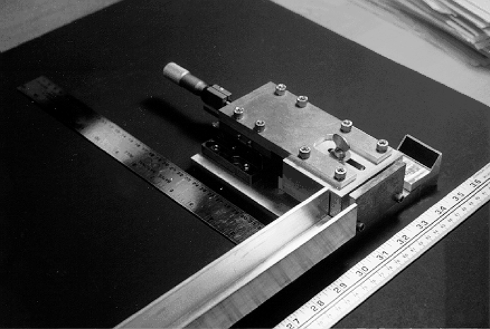
Fig. 11.— Pressing jig for gluing fiber arrays, based on a design by S. Barden. The inverted U‐shaped pressing channel (lower right) has a width controllable by a micrometer‐adjusted translation stage. A 45° mirror (middle right) is used for inspecting the fiber array during construction and curing. The lower diagonal rail is for holding the fiber cable, not used in practice. The entire jig is designed to be taken apart and cleaned between presses.
The entire process of laying down precision‐placed rows such that the bundle has little to no flare in the out‐of‐channel dimension requires skill and finesse that can only be accomplished through practice. Very small angular deviations from telecentricity can lead to substantial effective FRD, as illustrated in Fig. 12 (see also Wynne 1993). Hence, assuring that there is no flaring of the bundle is of utmost importance.
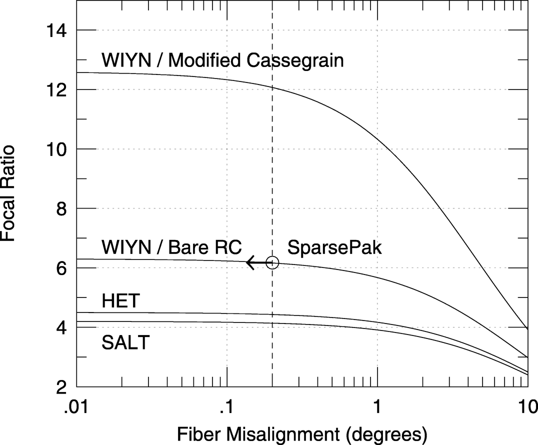
Fig. 12.— Focal‐ratio degradation due to fiber misalignment with the telecentric angle. The effective output f‐ratio of the extreme ray as a function of fiber misalignment from the optical axis (e.g., the telecentric angle) is shown for four input focal ratios: (1) the WIYN modified Cassegrain port (CassIAS) at f/13.5; (2) the WIYN Nasmyth (bare RC) port (IAS) at f/6.3; (3) the HET fiber instrument feed (FIF) at f/4.5; and the SALT fiber instrument feed at f/4.2. The effects are more pronounced for slower input beams, but in general substantial degradation occurs for misalignments above 0 1–0 3. The estimated alignment error budget for SparsePak is indicated by the vertical dashed line. In general, the effective output f‐ratio, as defined, e.g., by some EE, will also decrease with fiber misalignment, but at a slower rate, depending on the detailed shape of the input beam (see, e.g., Wynne 1993).
We use EPO‐TEK 354,18 a temperature‐curing epoxy. The heads were cured with a heat lamp in situ within the pressing jig and then released. In testing we found that despite liberal application of mold release, edge fibers were occasionally damaged or fractured. Consequently, we added a minimum of one row or column of short packing fibers to surround, or buffer, all elements of the science fiber arrays. As we show in § 6, we have found edge effects in the SparsePak array. On this basis we would now advocate a minimum of two, and ideally at least three, rows of packing fibers to act as a buffer.
A4. FIBER HEAD: POLISHING
Fiber‐head polishing was done using an Ultrapol 1200 polishing/lapping machine19 with 15.25 cm circular lapping disks.20 The polisher consists of a horizontal, rotating aluminum‐plated lubricant tub and a polishing head with a precision three‐axis positioner and oscillator. The lubricant of choice is distilled water. Many of the features on the costly positioner were unused, and in hindsight a custom‐made positioner would have been optimal for application with the heavier fiber arrays. In all cases fibers were attached via custom‐made aluminum adapters that directly attached to the polishing head. The fiber‐head adapter consisted of two 6.35 mm thick L‐shaped brackets that screwed together diagonally to place pressure on all four walls. To ensure the polished surface was orthogonal to the fiber length, support walls were connected to the L‐brackets (see Fig. 13).
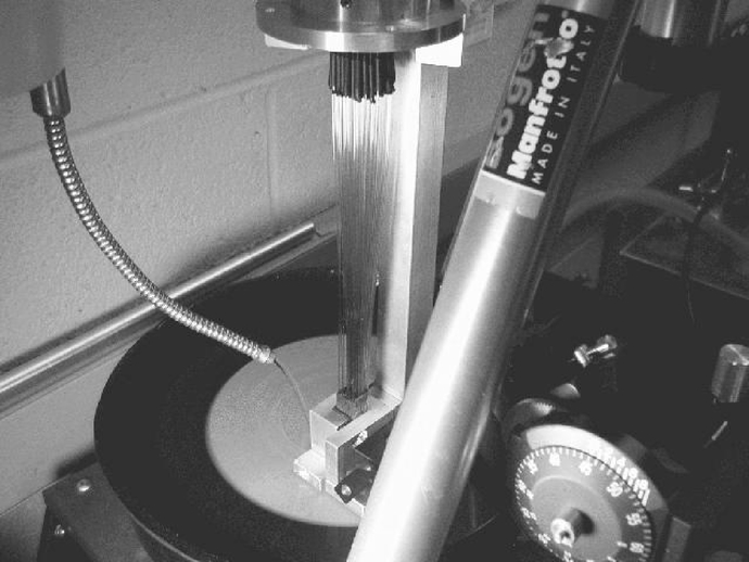
Fig. 13.— Close‐up view of the SparsePak head polishing in progress on the Ultrapol lap polisher. Note the vertical brace behind the bare fibers that extends from the double L‐bracket head attachment up to the cable termination. One of the L‐brackets has padded walls that serves to press the array against the other L‐bracket to form a precise, perpendicular alignment of the fiber array with the polishing surface. The other L‐bracket has U‐shaped slot (not seen) for attachment to the Ultrapol lapping polisher. The brace serves to prevent compression of the fibers during polishing. Lubricant is flowing through the flexible conduit onto the rotating platen containing a polishing disk. Also visible at lower right is the Ultrapol polishing arm with precision angle (roll and pitch) and height control. Given the load of the SparsePak cable, it was not feasible to use this feature during this stage of the polishing. Alignment of the fiber face perpendicular to the platen was made relative to the L‐bracket face. Note the leg of the camera tripod bearing the cable load. The cable is also supported by a sawhorse immediately to the left of the image.
Initial material was removed with coarse grit before we began true polishing. The polishing process consists of descending in grit size from 60, 40, 30, 15, 10, 5, and 1 (silicon carbide), and finally to 0.5 μm (aluminum oxide). For single fibers or small FFU heads made from thinner fibers, the oscillator could be used, greatly facilitating high‐grade polishing. A single fiber can take as little as an hour to polish, while a small FFU polishes in roughly 1–2 days. SparsePak head polishing took several weeks, because of the large area and quantity of material removed and the mechanical difficulty of manipulating the cable.
For example, because the cable was stiff and heavy, it had to be specially suspended and supported during polishing by a combination of sawhorse and camera tripod. A special brace was also made to directly connect the polishing head adapter to the cable termination to ensure fibers were not crushed (Fig. 13). Given these modifications, it was time consuming to remove and inspect the SparsePak head in midpolish, and nearly impossible to replace the head at exactly the same angle. Hence, small facets were introduced, and a "final" polish, while yielding excellent luster, still left several discrete scratches on the head surface visible at back‐lit, oblique angles at 10× magnification or higher. Horizontal polishing with the existing mount hardware was unsatisfactory for SparsePak.
We therefore developed a vertical hand‐polishing tool using two sets of precision ball slides21 to provide an X‐Y stage with 110 mm of diagonal travel (see the SparsePak Web site). A hand‐positioned, removable plunger with a 70 mm circular polishing surface allowed us to polish, remove, and inspect the SparsePak fiber head at regular and frequent intervals. (Lubricant is dropped vertically through the system while polishing.) With this polisher we were able to ensure perpendicularity of the polishing surface, remove remaining facets, and achieve a superior polish on the SparsePak surface. Despite these improvements, the final Sparsepak head face shows small microscratches on fibers 4, 16, 17, 24, 36, 40, and 72, even though the overall luster is high. Based on our lab measurements described in § 6, there is no evidence that these features diminish the throughput or degrade the output focal ratio by a measurable amount.
Our experience with EPO‐TEK 354 is that while its wicking properties are good, it does not polish as well as, e.g., Norland 68 UV curing epoxy.22 However, given the thickness of the SparsePak fiber head, a heat‐curing epoxy was essential.
A5. FIBER HEAD: MOUNT
SparsePak is designed to be swapped into and out of the WIYN Nasmyth IAS port on a regular basis. The terminal mechanical element in the SparsePak cable, the head mount, serves to grip the fiber head and provide a mounting surface. Reported here are salient details of what is required to provide a rigid and robust mounting mechanism compatible with existing interface hardware on the telescope.
A mounting box (WIFOE, named after the WIYN Fiber‐Optic Echelle), developed by K. Honneycutt and collaborators for a single fiber‐optic feed, is the mechanical assembly to which the SparsePak and DensePak attach during operation. WIFOE contains optics for feeding line lamps to the focal plane and for simultaneously viewing the back‐lit fiber face and focal‐plane image from the telescope. The WIFOE port requires a 25.4 mm OD tube of minimum length 44.4 mm, permitting a 17 mm maximum diameter for the fiber array, in order to maintain mechanical rigidity in the surrounding head mount. The SparePak fiber head diagonal dimension is at this limit.
The SparsePak fiber‐head mount (Fig. 14) was designed to ensure that the array was held at the proper telecentric angle if held rigidly by the WIFOE port. To do so we cut a 50.8 mm long channel in rectangular aluminum stock. The channel width matches the SparsePak fiber‐head width of 11.7 mm, with little (∼25 μm) clearance. The stock was then turned down to a 76.2 mm tube with a 25.4 mm diameter, and a 6.35 mm thick flange with a 50.8 mm OD for mounting to the rest of the cable. Three half‐clamshell clamps cover the channel. These units serve to give the tube a nearly complete circular cross section while at the same time providing the clamp mechanism for the array. The array was held with a uniform‐pressure rectangular clamp seated below the clamshells, actuated by three set screws in the clamshells. The fiber head is padded on both the top and bottom by a thin rubber gasket 38.1 mm in length. In this way, substantial force is exerted grabbing the fiber without substantially stressing the glass.
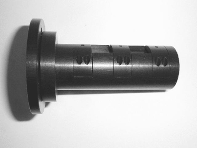
Fig. 14.— SparsePak fiber‐head mount. The fiber bundle inserts from the left and terminates 7.6 mm from the right end of the mount. Visible are the three clamshells, each with two pairs of mounting screws (near pair visible), and a set screw (top) that serves to press the clamping bar onto the array. The channel holding the array and bar is visible at the top.
To protect the fiber‐head face during installation and removal, the fiber head terminates roughly 7.6 mm back from the end of the mounting tube. This last portion of the mounting tube was beveled, ringed, sandblasted, and carefully flocked to avoid vignetting of the input beam on the edge fibers while minimizing glints and scattered light. Figure 15 is an image of the front face of the final assembled fiber head and mount.
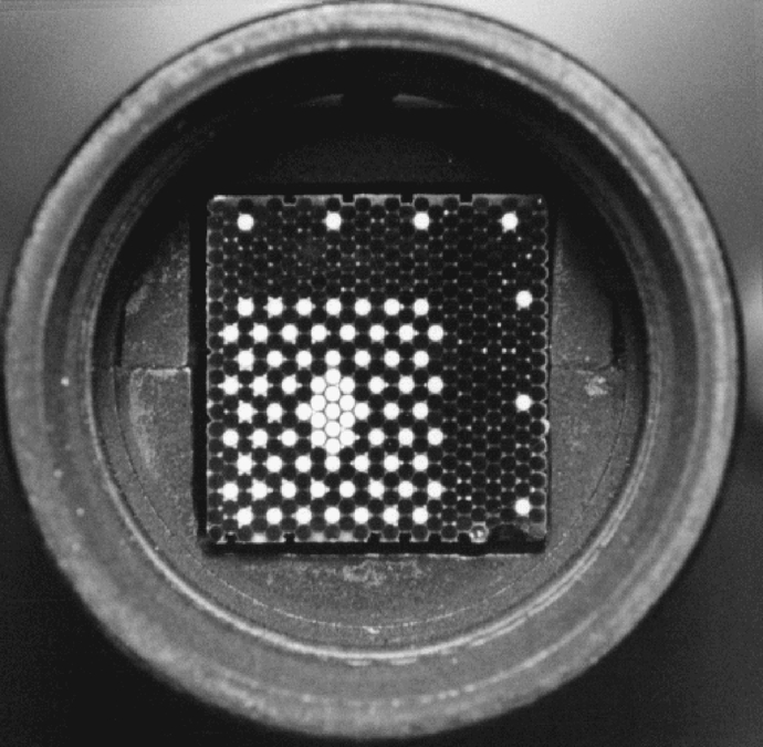
Fig. 15.— Final polished SparsePak head in its assembled head mount. The end of the head mount is beveled to avoid vignetting the outermost fibers for input f‐ratio slower than f/6; ridging and flocking is employed to help eliminate scattered light. Back‐illumination indicates the active (light) and short packing (dark) fibers. On‐sky orientation at the WIYN IAS port with zero rotator offset places north upward and east to the left (as also viewed in the WIFOE camera slit‐viewing camera).
The SparsePak fiber‐head mount is fastened in the WIFOE entrance collar with a thumb screw that sets into a detent. For a lightweight cable, such as one that contains a single fiber, this fastener is adequate both to firmly hold and retain the cable at the correct telecentric angle as the IAS rotates during observations. Because of SparsePak's considerable weight and rigidity, it was necessary to create a removable support flange. The flange attaches to the cable ∼33 cm back from the port collar and consists of a rigid, closed brace with a three‐leg attachment to the WIFOE and IAS. This modification eliminated remaining flexure to levels below detection and can also be used with DensePak.
The overall accuracy of the telecentric positioning of the fiber head is estimated to be better than 0 2, based on the quadrature sum of our estimates for (1) the accuracy of the positioning of the fiber head within the head mount (<0 15), and (2) the accuracy of the positioning of the head mount within the WIFOE collar (<0 15). Both of these estimates are based on the known mechanical tolerances of the mounting hardware. No accommodation is made in this estimate for any nonuniformities in the Nasmyth port mounts and WIFOE. The resulting increase in FRD, as illustrated in Figure 12, is under 3%.
A6. FIBER SLIT: MOUNT, ASSEMBLY, AND POLISHING
The slit assembly, containing all the elements after the shear clamp, consists of a 90° curved foot (Fig. 16) in which bare fibers make bends with radii between 82.6 and 178 mm, as well as a slit block and "toes" for filters and a slit‐narrowing mask. These are standard components required to integrate with the existing spectrograph mount. As shown in § 6, the curvature in this foot is problematic, a redesign of which, while beyond the scope and budget of this project, presents a clear upgrade path. However, we did make cost‐ and performance‐effective modifications to the toe and slit‐block design.
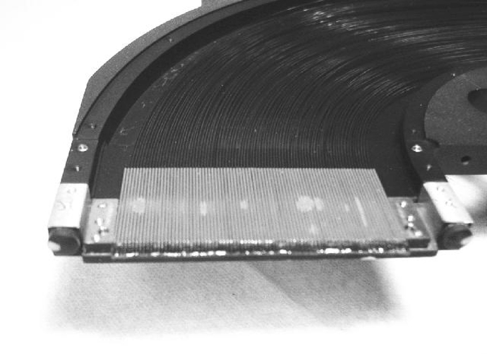
Fig. 16.— SparsePak fiber foot and slit block mounted into its polishing attachment (nonanodized end). While only the bottom portion of the fiber foot is visible in this image, the 90° bend of the fibers is clearly visible. The 32 mm long microtubes used for the slit block is at the bottom, with glued fibers protruding several millimeters from the end. During polishing and final assembly into the foot, a top clamp holds the slit block in place. The entire slit block clamping assembly is pinned into the foot to ensure precise location. The toes (not shown) extend from the end of the slit block toward the bottom and beyond the image.
We determined that the standard toe design produced substantial vignetting in the dimension transverse to the slit for on‐axis beams faster than f/5.7, and for beams faster than f/7.1 emanating from the edge of a 500 μm fiber. There is also vignetting in the dimension parallel to the slit for fibers near the ends of the slit; a slit‐edge fiber in SparsePak is vignetted for rays exiting faster than f/5.6. (For other feeds, the vignetting for edge fibers is more severe because of larger slit lengths—76.4 mm instead of 73.6 mm. This adds appreciably to their overall "slit function.") Given the f/6.3 input beam from the telescope, the output f‐ratio of the fibers is expected to be substantially faster than f/6, because of FRD. Hence, the SparsePak toes' chamber baffles were enlarged, and the last (fourth) chamber was removed. This enables an output beam at f/4 at the end of the slit for a 500 μm fiber to exit unvignetted from the feed; it provides room for simultaneous use of one interference and one glass filter; and is compatible with the existing mechanized filter‐insertion mechanism on the Bench.
The standard slit block consists of two clamp plates, one of which contains precision‐machined V‐grooves to locate microtubes, each containing a fiber. Such machining is difficult and expensive. We found that for 600 μm OD fibers, 20 gauge, thin‐wall stainless‐steel microtubes (31.8 mm in length, 647 μm ID, and 902 μm OD)23
provided an outstanding way to hold and separate the fibers if the tubes were tightly packed, like the fibers in a row of the FFU head. A packed row of 82 tubes yields a fiber‐to‐fiber edge separation of over 400 μm, and a total slit length of 73.6 mm from active fiber edge to edge. The glue thickness is inconsequential, since the microtubes were bonded in our pressing jig; the glue bonded in the interstitial regions. Our adopted slit block consisted of three rows of microtubes glued together for mechanical strength, pressed into a stainless‐steel holder, and pinned for precision alignment to the end of the fiber foot (see Fig. 16). We estimate that the overall alignment error of the fibers with respect to the optical mounting axis of the fiber foot is under 0 2.
The fibers themselves were bent, cut to final length, and then glued into the microtubes with only a bead of Norland 68 UV curing epoxy at the end of the tubes. They were then cured using a commercial black light. The entire slit block, which was attached to the fiber foot, was mounted on our Ultrapol lapping machine with a special adapter. It polished well and did not require additional hand‐polishing. This concluded the SparsePak cable manufacture.
A7. TOTAL EFFORT
For reference for future efforts: the cable construction and fiber installation took ∼320 person‐hours (two people at any given time, except for hauling the cable—a half‐hour process requiring four people), and 1 month of shop time for fittings and termination hardware. Polishing took an additional person‐month, plus one week of shop time. These totals do not include the more substantial effort to develop the assembly, gluing and polishing techniques, nor does it include time for the laboratory calibration measurements described in § 6.
Footnotes
- 6
This assumes a telescope clear aperture with an effective diameter of 3.186 m based on a 3.499 m diameter primary and a central obstruction diameter of 1.446 m, as listed on http://claret.kpno.noao.edu/wiyn/wiynfacts.html.
- 7
- 8
The effective clear apertures are 235 mm diameter for the collimator, 203 × 406 mm for the echelle, 203 × 230 mm for the low‐order gratings, and 206 mm diameter for the camera. The projected grating areas for on‐order settings with the nominal camera collimator angles are roughly 205 × 210 mm for the low‐order gratings blazed below 25°, and only 205 × 165 mm for the echelle and low‐order gratings blazed above 25°.
- 9
These include the red and blue Hydra MOS cables, DensePak, and now SparsePak.
- 10
Not considered here is an additional source of error, relevant to high‐signal regimes, from imperfect pixel‐by‐pixel correction of the CCD response (i.e., field‐flattening).
- 11
The width dimension is defined as the 23 rows in the direction orthogonal to the major axis of the central densely packed fibers. Mechanically, the width is in the direction of the cut in the head mount that forms the clamp. The height dimension is defined as the 20 rows in the direction parallel to major axis of the central densely packed fibers. Mechanically, the width is in the direction orthogonal to the cut in the head mount that forms the clamp.
- 12
- 13
Precision Instrumentation and Software, Santa Barbara, CA.
- 14
Polymicro Technologies Incorporated, 18019 North 25th Street, Phoenix, AZ 85023‐1200.
- 15
Zeus, P.O. Box 2167, 620 Magnolia Street, Orangeburg, SC 2911‐2167.
- 16
McMaster‐Carr Supply Co., P.O. Box 94930, Cleveland, OH 44101‐4930.
- 17
Miller‐Stephenson Chemical Co., Inc., 55 Backus Avenue, Danbury, CT 06810.
- 18
Epoxy Technology, Inc., 14 Fortune Drive, Billerica, MA 01821.
- 19
Ultra Tech, 1025 East Chestnut Avenue, Santa Anna, CA 92701‐6491.
- 20
Moyco Industries, Inc., Corporate Offices & Ultralap/Abrasives Division, 200 Commerce Drive, Montgomeryville, PA 18936.
- 21
Del Tron Precision, Inc., 5 Trowbridge Drive, P.O. Box 505, Bethel, CT 06801.
- 22
Norland Products, Inc., P.O. Box 637‐T, Cranbury, NJ, 08512.
- 23
Connecticut Hypodermics, 519 Main Street, Yalesville, CT 06492.