
ABSTRACT
We present the results of monitoring optical‐turbulence profiles at San Pedro Mártir, Mexico, during 11 nights in 1997 March and April, and 16 nights in 2000 May. The data were collected using the generalized scintillation detection and ranging (SCIDAR) technique from Nice University at the 1.5 and 2.1 m telescopes. A total of 6414 turbulence profiles were measured and statistically analyzed. The principal results are as follows: the seeing produced by the turbulence in the first 1.2 km at the 1.5 m and 2.1 m telescopes, not including turbulence inside the domes, have median values of 0 63 ± 001 and 044 ± 002, respectively. The dome seeing at those telescopes have median values of 064 ± 001 and 031 ± 002. The median values of the seeing produced above 1.2 km and in the whole atmosphere are 039 ± 001 and 071 ± 001. The isoplanatic angle for full‐correction adaptive optics has a median value of 187 ± 004. The decorrelation time (defined as the time lag for which the temporal correlation drops to 50%) of the turbulence strength at altitudes below and above 16 km above sea level is approximately equal to 2 and 0.5 hr, respectively. The isoplanatic‐angle decorrelation time is estimated to be equal to 2 hr. The turbulence above ∼8 km remained notably calm during nine consecutive nights, which is encouraging for adaptive optics observations at the site. The results obtained here places San Pedro Mártir among the best suited sites for installing next‐generation optical telescopes.
Export citation and abstract BibTeX RIS
1. INTRODUCTION
The development of next‐generation adaptive optics systems for existing or future telescopes requires a precise characterization of on‐site atmospheric turbulence. Not only are the seeing statistics needed, but also those of the vertical distribution of the refractive‐index structure constant C2N(h). For example, the design of multiconjugate adaptive optics (MCAOs; systems that incorporate several deformable mirrors, each conjugated at a different altitude) requires knowledge of the statistical behavior of the optical turbulence in the atmosphere, such as the altitude of the predominant turbulent layers and their temporal variability. Moreover, the selection of sites where the next‐generation ground‐based telescopes are to be installed first requires reliable studies of the C2N profiles at those sites.
These reasons have motivated two observing campaigns at the Observatorio Astronómico Nacional de San Pedro Mártir (OAN‐SPM), during which the C2N profiles were monitored. The campaigns took place in 1997 (March and April) and 2000 (May), for a total of 27 nights. The measurements were performed using the generalized SCIDAR (GS) from Nice University, which was installed on the 1.5 and 2.1 m telescopes (hereafter SPM1.5 and SPM2.1). The instrument also provided the velocity of the turbulent layers, which were measured simultaneously with the C2N profiles.
Here we present the main results obtained from the C2N(h) measurements performed during these campaigns. A forthcoming article will be devoted to the results concerning the turbulent‐layer velocities. Avila et al. (1998) reported the C2N(h) results from the 1997 observations alone. Section 2 briefly presents the measurement techniques and the observation campaigns. An overview of the monitored turbulence profiles is given in § 3, and the statistical analysis of the C2N vertical distribution is presented in § 4. The temporal behavior of C2N(h) and that of the isoplanatic angle are studied in § 5. Section 6 gives a summary of the results. Finally, in Appendix
2. MEASUREMENTS OF C2N PROFILES
2.1. GS Generalities
The method used to monitor the turbulence profiles was the generalized SCIDAR (Rocca et al. 1974; Avila et al. 1997; Fuchs et al. 1998). Details of the instrumental concept, together with a complete bibliography, can be found on the Web page entitled "Generalized Scidar at UNAM."2 Here we give a very succinct description of the instrument and data‐reduction procedure.
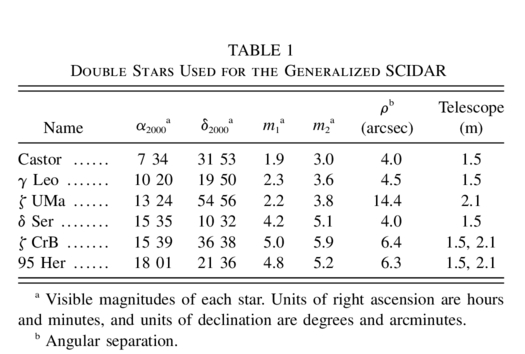
The instrumental concept consists of the measurement of the spatial autocorrelation of double‐star scintillation images detected on a virtual plane a few kilometers below the ground. The exposure time of each image is 1 or 2 ms, depending on the stars' magnitudes and the prevailing observing conditions. The wavelength is centered at 0.5 μm. A 128 × 128 autocorrelation map is saved on disk at time intervals that depend on the number of images used to compute the autocorrelation. During the 1997 campaign, 1000 images were generally used, while in the 2000 campaign that number was generally set to 2000, which gave mean time lags between registrations of 0.56 and 1.32 minutes, respectively. The double stars used as light sources in each telescope during the 1997 and 2000 campaigns are listed in Table 1. The data shown in this table were obtained from the Washington Double Star Catalog (Mason et al. 2002). Many of the sources are multiple systems, but in each case our instrument is only sensitive to the primary and secondary components. In some cases, the autocorrelation maps show diagonal bands that are parallel to each other, which are produced by video noise on the scintillation images. In such cases, the maps have been passed through a filter that eliminates or attenuates the bands. If the noise is still significant after filtering, the maps are rejected. From each retained map, one C2N profile is retrieved using a maximum‐entropy algorithm to invert an integral ill‐posed equation. The vertical resolution of each C2N profile depends on the star separation ρ and the zenith angle z through
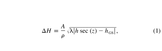
where λ is the wavelength, h is the altitude above the ground, and hGS is the virtual distance from the pupil to the detector conjugated plane. The factor A varies from 0.5 to 0.78, depending on the criterion used to define the width of the theoretical spatial autocorrelation function of the scintillation produced by a layer at altitude h (Vernin & Azouit 1983; Avila et al. 1998; Prieur et al. 2001). Following Avila et al. (1998), we adopted A = 0.5. In order to have a C2N(h) data set with a regular altitude sampling, all the profiles were resampled to an altitude resolution of 500 m.
 |
2.2. Observing Campaigns
The OAN‐SPM, operated by the Instituto de Astronomía of the Universidad Nacional Autónoma de México, is situated on the Baja California peninsula at 31°02' north, 115°29' west, and at an altitude of 2800 m above sea level. It lies within the northeastern part of the San Pedro Mártir (SPM) National Park, at the summit of the SPM sierra. Cruz‐González et al. (2003) has collected in one volume all the site characteristics studied so far.
In the 1997 observing campaign, the GS was installed on SPM1.5 and SPM2.1 for eight and three nights, respectively (1997 March 23–30 and April 20–22 UT). SPM2.1 is installed on top of a 20 m tall building at the summit of the mountain (2850 m above sea level) in such a way that no obstacles generate ground turbulence. On the other hand, SPM1.5 is constructed closer to ground level, on a site situated below the summit. The results of this campaign were presented by Avila et al. (1998).
The 2000 campaign took place May 7 through 22 UT. A number of instruments were deployed, but for the purpose of the present article, it suffices to say that the GS was installed during 9 and 7 nights (May 7–15 and 16–22 UT) on SPM1.5 and SPM2.1, respectively. Masciadri et al. (2004) and Avila et al. (2002) describe the complete set of instruments used in that campaign, which provided the data for the calibration and validation of the Meso‐NH atmospheric model for the three‐dimensional simulation of C2N (Masciadri et al. 2004). Some of these measurements also led to a study of the contribution of the surface layer to the seeing (Sánchez et al. 2004).
3. C2N(h) DATA OVERVIEW
The number of turbulence profiles measured in the 1997 and 2000 campaigns are 3398 and 3016, respectively, making a total of 6414 estimations of C2N(h). All the profiles refer to altitudes above sea level (2800 m at OAN‐SPM). Figure 1 shows the C2N profiles obtained during the 2000 campaign. The mean temporal sampling is 1.32 minutes (see § 2.1). The aim of that figure is only to give the reader a sense of the evolution of the turbulence profiles during each night and from night to night, so only the 2000 profiles are shown. The three upper rows correspond to the data obtained with SPM1.5. The two last rows show data obtained with SPM2.1. The first SPM2.1 night was cloudy. The blank zones correspond to either technical problems, clouds, or source changes. The C2N values for altitudes within the observatory and 1 km lower are to be taken as part of the response of the instrument to turbulence at the observatory level. For altitudes lower than that, the C2N values are artifacts of the inversion procedure and should be ignored (Avila et al. 1997).
Generally, the most intense turbulence is located at the level of the observatory, where contributions from inside and outside of the telescope dome are added. In the statistical analysis presented in § 4, dome turbulence is subtracted. The profiles obtained with the SPM2.1 in 2000 show a fairly stable and strong layer between 10 and 15 km, corresponding to the tropopause (as deduced from the balloon data). This layer is rarely present in the data obtained with the SPM1.5 in the same year. Sporadic bursts of turbulence are noticed at altitudes higher than 15 km.
4. STATISTICS ON THE C2N VERTICAL DISTRIBUTION
4.1. Dome Seeing
All the raw C2N profiles, as those shown in Figure 1, include in the ground‐level values both the atmospheric ground layer and the turbulence inside the telescope dome. For the characterization of the site, we needed to remove the dome seeing contribution from the profiles. The method used to estimate the dome C2N is explained in detail by Avila et al. (2001), and some improvements (not implemented here) are suggested by Masciadri et al. (2004). Here we briefly summarize the method used.
The estimation of the dome seeing is obtained from the analysis of the GS measurements of the cross‐correlation of double‐star scintillation maps taken at temporal intervals Δt. The cross‐correlation is calculated using the same frames as those used for the computation of the autocorrelation. The cross‐correlation produced by each turbulent layer consists of three peaks (the so‐called "triplets"). The position of the central peak with respect to the origin (center of the cross‐correlation plane) and the knowledge of Δt give us the velocity vector (intensity and direction) of the detected turbulent layer. The separation of the lateral peaks (d = ρ|h - hGS|) with respect to the central one gives us the altitude h of the layer with respect to the ground. We define H = |h - hGS| (in our case, hGS = -3000 or −4000 m). The seeing inside the dome is characterized by turbulence with a mean velocity V = 0, so the triplet is placed at the origin ± ΔV (where ΔV is the velocity resolution of the instrument). The position of the central peak at the origin is a necessary but not sufficient condition to determine the dome contribution. Because of the relatively low vertical resolution of the GS, some turbulence in the boundary layer, external to the dome and characterized by a mean velocity smaller than ΔV, could be associated with a triplet such as the one just described. The only case in which we can be reasonably sure that the detected triplet is associated with turbulence inside the dome is when at least two triplets are detected at the same altitude h = 0 ± ΔH/2 (where ΔH is defined by eq. [1]): one is characterized by V<ΔV (which is associated with dome turbulence), and another one by V>ΔV (corresponding to turbulence outside of the dome). In the case in which only one triplet at altitude h = 0 ± ΔH/2 is encountered, the dome seeing detection is labeled "ambiguous" and is not taken into account. The value of C2NΔH inside the dome is set equal to αaC2N(h = 0)ΔH/(a + b), where a is the amplitude of the central peak with h = 0 ± ΔH/2 and V = 0 ± ΔV, b is the sum of the amplitudes of the central peaks with h = 0 ± ΔH/2 and V>0 ± ΔV (note that sometimes there is only one such triplet), and α is the factor that accounts for the slower temporal decorrelation of the turbulence inside the dome than that from outside. We have estimated experimentally that α = 0.87.
The dome seeing was determined for 84% of the profiles measured during the 2000 campaign. In the remaining 16% of the profiles, the determination of the dome seeing was "ambiguous," so we did not include these data in the dome seeing database. For the 1997 data, only a few values of the dome seeing were obtained each night.
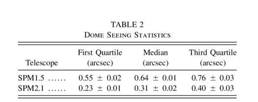
Figure 2 represents the cumulative distribution functions of the dome seeing values that were obtained. Table 2 gives the median values and first and third quartiles. The calculation of the uncertainties of these statistical values is explained in
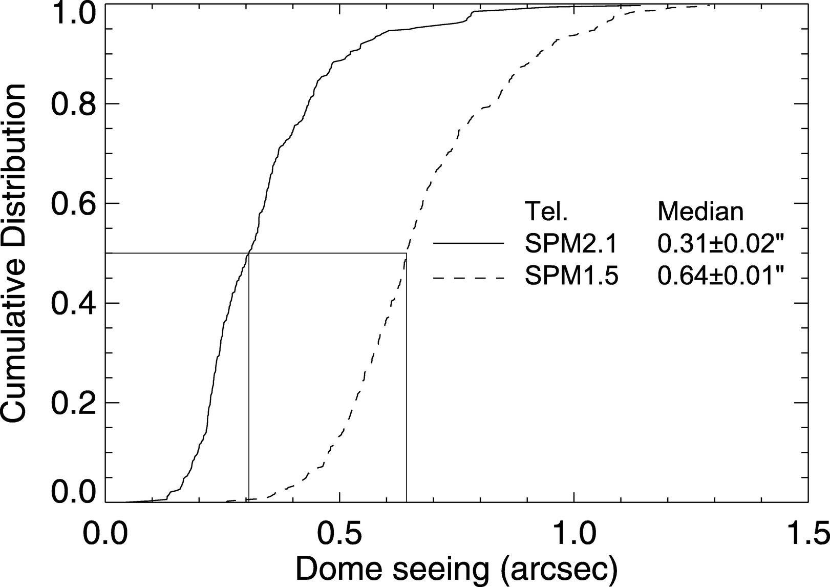
Fig. 2.— Cumulative distribution of the seeing generated inside the dome of SPM2.1 (solid line) and SPM1.5 (dashed line). Data used are from 1997 and 2000 campaigns. The vertical and horizontal lines indicate the median values. These values, together with the first and third quartiles, are reported in Table 2.
 |
In the remainder of this paper, all the statistical results concerning the turbulence near the ground are free of dome turbulence. In the case of the profiles for which the dome C2N was not determined, the median value of the dome C2N for the corresponding telescope was subtracted.
4.2. Median Profiles
The median and first and third quartile values of C2N(h) obtained with SPM1.5 and SPM2.1 are shown in Figures 3a and 3b, respectively. These profiles were computed using the data from both campaigns (i.e., the complete GS data set), with the dome seeing removed. An interesting resulting characteristic is that the turbulence measured at the telescope level is notably more intense at SPM1.5 than at SPM2.1. We believe that this is principally due to the fact that SPM1.5 is located at ground level, while SPM2.1 is installed on top of a 20 m building. Moreover, the SPM2.1 building is situated at the observatory summit, whereas SPM1.5 is located at a lower altitude. Figure 3c shows the median profile calculated from all the C2N profiles measured with the GS at the OAN‐SPM (i.e., both campaigns and both telescopes).
Another difference seen in the median profiles obtained with SPM1.5 and SPM2.1 (Figs. 3a and 3b) is that the tropopause layer, which is centered at approximately 12 km, is much stronger in Figure 3b than in Figure 3a. This is not a consequence of the individual telescope used. By chance, it happened that while observing with SPM1.5 during the 2000 campaign, the turbulence at that altitude—and everywhere higher than 8 km—was very weak, as seen in Figure 4. During that campaign, between the SPM1.5 and SPM2.1 observations, there was one cloudy night. In contrast to the first nine nights of the campaign (when the GS was installed on SPM1.5), during the first observable night on SPM2.1, the turbulence in the tropopause was extremely intense. This can be seen in the first cell of the fourth row of Figure 1. It is often believed that turbulence intensity in the tropopause at medium‐latitude sites is systematically strong. The median profile in Figure 4 demonstrates that this is not always true. The turbulence above ∼8 km during the first nine nights of the 2000 campaign remained notably calm. Tokovinin et al. (2003) also noted a 4 day period of calm free‐atmosphere turbulence above Cerro Tololo, Chile, which is consistent with our results.
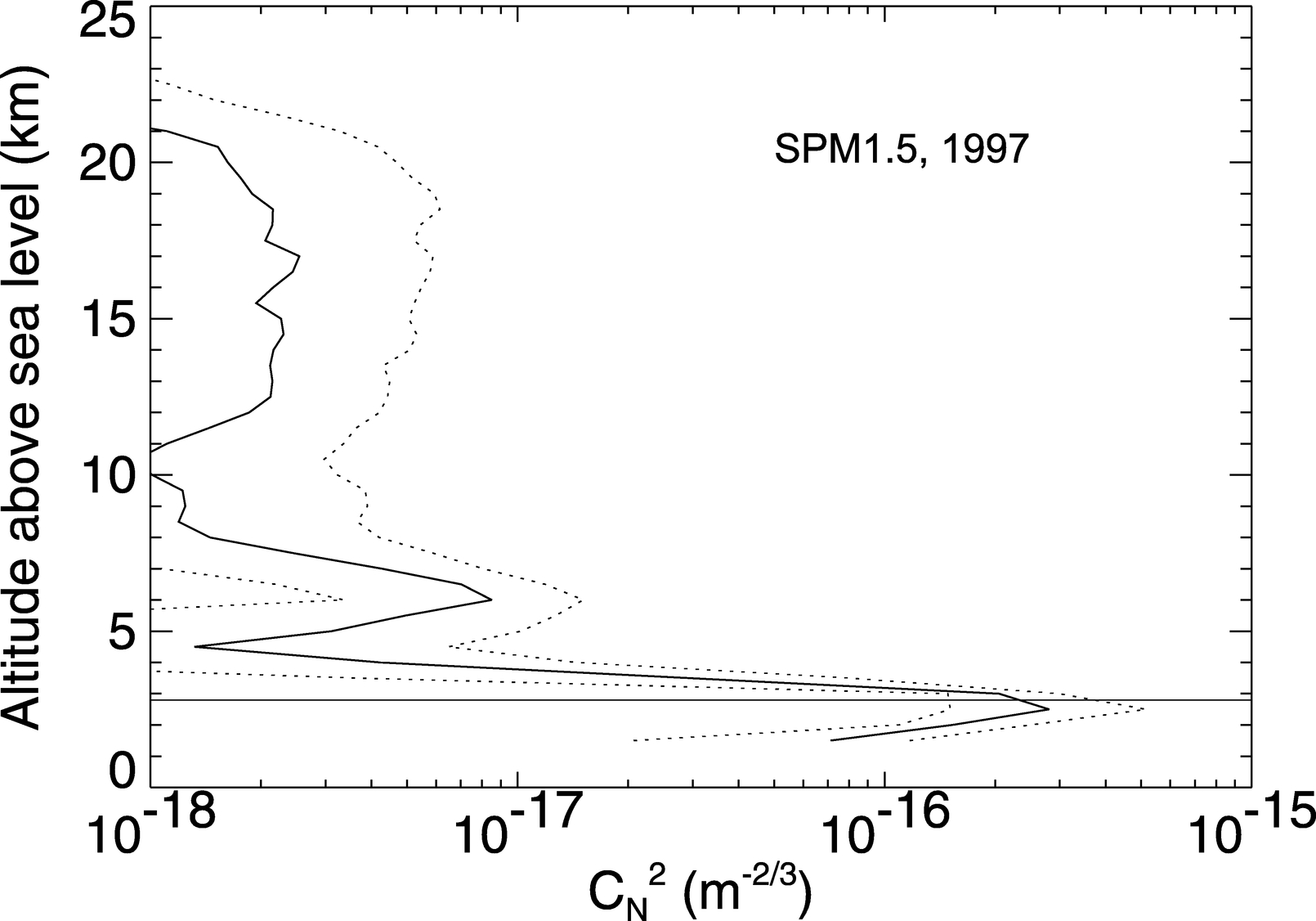
Fig. 4.— Similar to Fig. 3, but for the GS profiles obtained at SPM1.5 during the 2000 campaign.
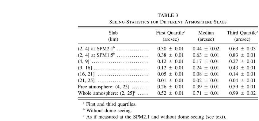
4.3. Seeing for Different Atmospheric Slabs
From a visual examination of Figure 1, we can determine five altitude slabs that contain the predominant turbulent layers. These are (2, 4], (4, 9], (9, 16], (16, 21], and (21, 25] km above sea level. In each altitude interval of the form (hl, hu] (where the subscripts l and u stand for lower and upper limits, respectively) and for each profile, we calculate the turbulence factor
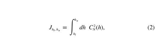
and the corresponding seeing in arcseconds,
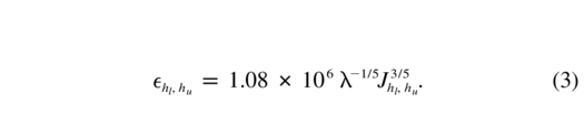
For the turbulence factor corresponding to the ground layer J2,4, the integral begins at 2 km in order to include the complete C2N peak that is due to turbulence ground level (2.8 km). Moreover, J2,4 does not include dome turbulence. The seeing values have been calculated for λ = 0.5 μm. Figure 5a shows the cumulative distribution functions of  2,4, which were obtained at SPM1.5 and SPM2.1 and calculated using the complete data set. As discussed in § 4.2, the turbulence at ground level at SPM1.5 is stronger than that at SPM2.1. The cumulative distributions of the seeing originating in the four slabs of the free atmosphere (from 4 to 25 km) are represented in Figure 5b. Table 3 gives the first, second, and third quartile values of the distributions shown in Figure 5. The largest median seeing in the free atmosphere is encountered from 9 to 16 km, where the tropopause layer is located. In addition, the dynamical range of seeing values in that slab is the largest, as can be noted from the first and third quartiles (012 ± 001 and 043 ± 001). Particularly noticeable is the fact that the seeing in the tropopause can be very small (see § 4.2), as indicated by the left tail of the cumulative distribution function of 9,16. The turbulence at altitudes higher than 16 km is fairly weak. Finally, Figures 6a and 6b show the cumulative distribution of the seeing produced in the free atmosphere, 4,25, and in the whole atmosphere, 2,25, respectively. The computation of 2,25 is performed as follows: for each profile of the complete data set (both campaigns and both telescopes), we calculate J4,25 and add a random number that follows the same lognormal distribution as that of the J2,4 values measured at SPM2.1 in 1997 and 2000. Then the corresponding seeing value is calculated using equation (3). This way, we obtain a distribution of 2,25 values as if they were measured using SPM2.1. The reason for doing so is that the values of 2,25 that we obtain are more representative of the potentialities of the site than if we had used the distribution of J2,4 obtained for SPM1.5. The median values of all the cumulative distributions presented in this section are reported in Table 3.
 |
4.4. Isoplanatic Angle
From each C2N profile of both campaigns, one value of the isoplanatic angle θ 0 (Fried 1982) has been computed using the expression

where r0 is the Fried parameter (Fried 1966), defined as
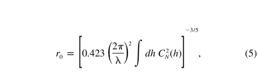
and
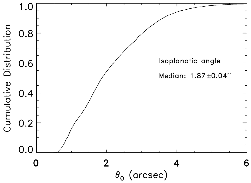
The cumulative distribution function of θ 0 is shown in Figure 7. The first, second, and third quartile values are equal to 125 ± 004, 187 ± 004, and 281 ± 004, respectively.
5. TEMPORAL AUTOCORRELATION
What are the characteristic temporal scales of the fluctuations of optical turbulence at different altitudes in the atmosphere? This question has been of interest for a long time, particularly in recent years, since the development of MCAOs require knowledge of the properties of the optical turbulence in a number of slabs in the atmosphere. Racine (1996) studied the temporal relative fluctuations of free‐atmosphere seeing above Mauna Kea. He computed the seeing values by integrating turbulence profiles measured in 1987 by Vernin's group from Nice University using the SCIDAR technique. The C2N profiles did not include the turbulence from the first kilometer, because the classical mode of the SCIDAR was employed (as the generalized mode did not exist at the time). Muñoz‐Tuñón et al. (1997) used differential image motion monitor (DIMM) data to study the temporal behavior of the open‐air seeing at Roque de Los Muchachos observatory. Finally, Tokovinin et al. (2003) presented the temporal autocorrelation of the turbulence factor in three representative slabs of the atmosphere above Cerro Tololo Interamerican Observatory using data obtained with the recently developed multiaperture scintillation sensor (MASS), which provides C2N measurements at six altitudes in the atmosphere. Details of the methods followed in these investigations are given in § 5.1.
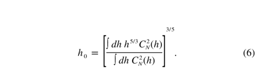
Also of great importance is the characteristic temporal scale of the isoplanatic‐angle fluctuations. One would expect this parameter to be governed by the temporal evolution of the C2N in the strongest turbulence layers above the site (apart from the ground layer), regardless of its altitude, because the influence of the C2N(h) term on h0 (see eq. [6]) is more important than that of h. Indeed, C2N(h) may vary over at least 2 orders of magnitude as a function of h, whereas h5/3 only varies over a factor of about 38 (∼[25/2.8]5/3). Nevertheless, it is interesting to directly calculate the temporal autocorrelation function of θ 0 in order to verify the reasoning above and obtain a quantitative result. It is worth mentioning that such a study has never before been published.
In this section we investigate the temporal autocorrelation of the turbulence factors Jhl,hu for the five slabs introduced in § 4.3, and also present the temporal autocorrelation of the isoplanatic angle θ 0.
5.1. Methodology
The process of building the appropriate sequences of Jhl,hu(ti) values is explained below.
Typically, three stars are used as light sources each night in a sequence such that the zenith angle never exceeds ∼40°. When changing from one star to another, the region of the atmosphere that is sensed by the instrument changes significantly, and so C2N(h) can also change, as shown by Masciadri et al. (2002). To avoid confusion between a temporal and spatial variation of Jhl,hu, the sequences Jhl,hu(ti) never include data obtained with two different stars. Moreover, we chose to build sequences made of at least 3 hr data sets that contained interruptions not longer than 30 minutes, in order to obtain temporal autocorrelation values with acceptable signal‐to‐noise ratios. These conditions were not met by the C2N profiles measured in 1997, so in this study only data from the 2000 campaign were used.
We built 35 sequences Jhl,hu(ti) for each of the five altitude intervals. The temporal sampling of the turbulence profiles depends on the number of scintillation images recorded for the computation of each profile, which in turn depends on the source magnitude. Consequently, each sequence Jhl,hu(ti) is resampled with a regular time interval of δt = 1.32 minutes, which is the mean temporal sampling of the C2N profiles used in this study. Moreover, while observing a given source, the data acquisition might be interrupted. If the interruption is longer than 2δt, the temporal gap is then filled with zero values for Jhl,hu(ti), and the data are not considered, as explained below.
For each altitude interval, the calculation of the temporal autocorrelation, as a function of the temporal lag Δt, is performed as follows. For each Jhl,hu sequence labeled s, we first compute
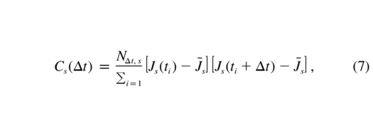
where the product is set equal to zero if either Js(ti) = 0 or Js(ti + Δt) = 0. Here J s is the mean of the nonzero values of Js(ti), and NΔt,s is the number of computed nonzero products, which depends on Δt and the number of nonzero values of Js(ti) in the sequence s and is calculated numerically. The autocorrelation for each altitude slab is then given by
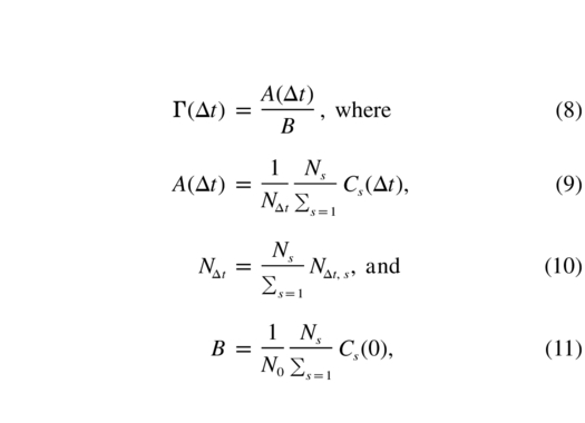
where Ns is the number of sequences for each altitude interval, and N0 is equal to NΔt for Δt = 0. From the definitions of Cs(Δt) and NΔt (eqs. [7] and [10]), it can be seen that the normalization factor B only takes into account nonzero values of Js(ti).
This method is similar to that used by Tokovinin et al. (2003), except for the fact that these authors calculate
instead of Cs(Δt) of equation (7). Both equations are mathematically equivalent as long as J s is computed with an infinite number of samples. We found that in our case, equations (7) and (12) give nonnegligible differences, so we chose to use equation (7), on which the definition of the autocorrelation function is based (Natrella 2004). An analogous remark applies for the method used by Muñoz‐Tuñón et al. (1997). In the case of Racine (1996), the author calculates the function
where the notation 〈...〉 represents an average over t. This function represents the characteristic fractional change of Js as a function of the time lag Δt, which has a different meaning from that of the temporal autocorrelation function. As mentioned above, Racine (1996) performed his study only on the free‐atmosphere seeing. Avila et al. (2003) studied fs(Δt) for the five altitude slabs considered here, using part of the C2N profiles of the 2000 campaign.
The calculation of the autocorrelation of θ 0, which we call Γθ 0(Δt), is performed in the same manner as that of Γ(Δt). One just has to replace Js by θ 0 in equation (7) to obtain Γθ 0(Δt) in equation (8).
5.2. Results
The temporal autocorrelations for the five atmosphere slabs were computed using the 2000 campaign data set, as explained in § 5.1. The turbulence inside the dome was removed. The number NΔt of products summed to calculate Γ(Δt) ranges from ∼2902 for Δt = 0 to ∼870 for Δt = 3 hr. The results are shown in Figure 8. For every slab, the autocorrelation shows a steep descent for short temporal lags (Δt≲0.2 hr), followed by a less rapid decrease for longer lags. It can be seen that in the first three altitude slabs, the turbulence decorrelates more slowly than in the two higher slabs. The time lags for a 50% decorrelation are approximately 2, 2.5, 1.7, 0.7, and 0.2 hr in the altitude ranges (2, 4], (4, 9], (9, 16], (16, 21], and (21, 25] km, respectively. The turbulence in the highest slab is so weak (as seen in Fig. 5) that Γ(Δt) for that slab might be strongly affected by the temporally decorrelated noise variations. Turbulence in the highest layers evolves more rapidly than in the lower layers, but introduces fewer distortions in the wave front because they are weaker. In the altitude ranges (2, 4] and (9, 16] km, the turbulence is the most intense, but fortunately the variations are slow. The counterbalance of these effects is evident in the temporal autocorrelation of the isoplanatic angle shown in Figure 9. Although the highest layers contribute the most to the decrease in the isoplanatic angle, the time lag for a 50% decorrelation of θ (∼2 hr) is similar to that of the turbulence located below 16 km, where the most intense turbulence is found. This is the expected behavior, as mentioned in § 5.
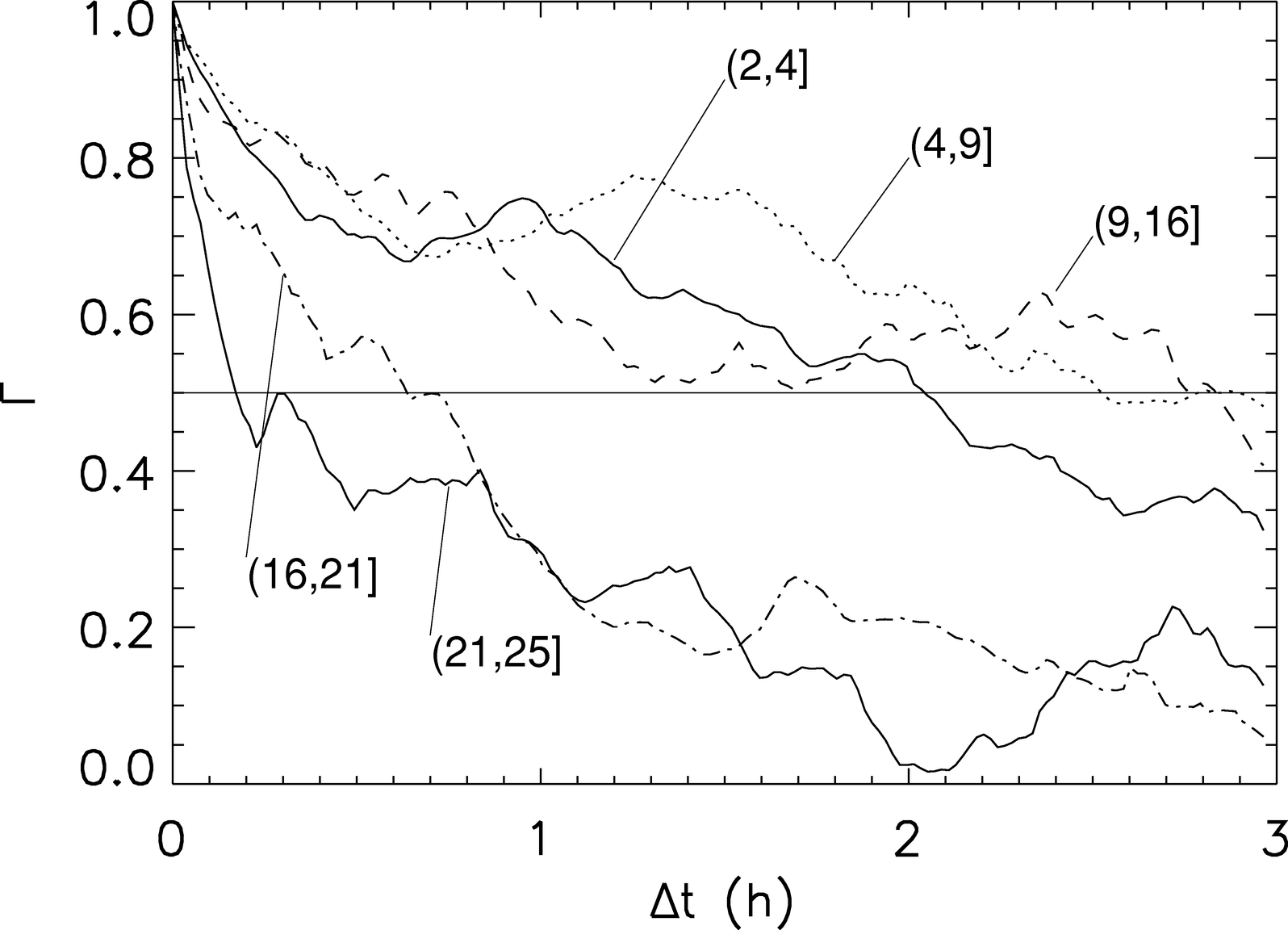
Fig. 8.— Temporal autocorrelation of the turbulence factor Jhl,hu(ti) for the intervals (hl,hu] km indicated in the figure. Data used are from the 2000 campaign.
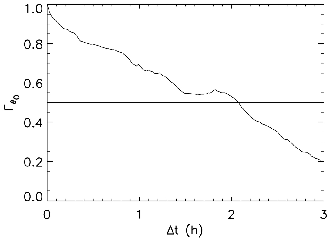
Fig. 9.— Temporal autocorrelation of the isoplanatic angle θ 0. Data used are from the 2000 campaign. The 50% decorrelation time is about 2 hr.
Intriguingly, our results show that in the free atmosphere, the C2N decorrelates more rapidly as the altitude increases, which seems to contradict the results of Tokovinin et al. (2003). These authors found that the 50% decorrelation time of the C2N in the layers situated at 1, 4, and 16 km above Cerro Tololo is equal to 0.3, 1.6, and 1.9 hr, respectively. It would be interesting to determine if such a difference is a consequence of the fact that the measurements were taken at different sites, at different epochs, or if it depends on the instrument used to measure C2N(h) (Tokovinin et al. 2003 used a MASS).
Muñoz‐Tuñón et al. (1997) found a characteristic decorrelation time of 1.2 hr for the open‐air seeing above Observatorio Roque de los Muchachos, Canary Island, Spain. The value they report is in agreement with the values obtained here for the altitude slabs for which the turbulence is most intense (below 16 km).
6. SUMMARY AND CONCLUSIONS
Turbulence profiles have been monitored at the OAN‐SPM during 11 nights in 1997 April–May and 16 nights in 2000 May. The GS was installed at the foci of SPM1.5 and SPM2.1. Turbulence inside the dome was detected by the instrument, but for each profile, this contribution has been estimated and separated from the turbulence near the ground outside the dome. The result is a data set consisting of two subsets: turbulence profiles free of dome seeing, and dome seeing values. From the statistical analysis of this data set, we draw the following conclusions:
- 1.The turbulence inside SPM1.5 is much stronger than that at SPM2.1, with median values of 064 ± 001 and 031 ± 002.
- 2.The precise location of each telescope influences the turbulence measured near the ground. SPM1.5 is installed basically at ground level and is lower than the site summit, while SPM2.1 is on top of a 20 m building at the site summit. A consequence of this is that the median values of the seeing produced in the first 1.2 km are 063 ± 001 and 044 ± 002 for SPM1.5 and SPM2.1, respectively.
- 3.The seeing generated in the free atmosphere (above 1.2 km from the site) has a median value of 039 ± 001. This very low value encourages adaptive optics observations, since the lower the turbulence in the higher layers, the broader is the corrected field of view.
- 4.The seeing in the whole atmosphere without the dome contribution as measured from SPM2.1 has a median value of 071 ± 001.
- 5.The temporal autocorrelation of the turbulence factors Jhl,hu (see § 4.3) shows that C2N evolves sensibly more slowly in the layers below 16 km (above sea level) than in the layers above that altitude. The time lag corresponding to a 50% decorrelation is approximately equal to 2 and 0.5 hr for turbulence below and above 16 km, respectively. The longer the 50% decorrelation time, the higher the potential performances of adaptive‐optics observations are, and the easier would be the development of multiconjugate adaptive optics systems. The rapid evolution of the C2N in the highest layers is, in principle, a negative behavior. However, this is counterbalanced by the very low C2N values in those layers.
- The isoplanatic angle has a characteristic 50% decorrelation time of approximately 2 hr, which is similar to that of the turbulence below 16 km. This is the first time that the isoplanatic‐angle decorrelation function has been estimated experimentally.
The C2N profiles are extremely important for choosing a site for an extremely large telescope (ELT) or any optical telescope equipped with adaptive optics. The studies performed at the OAN‐SPM have revealed that the site has truly excellent turbulence conditions. However, longer term monitoring is desirable, in order to confirm our results and identify seasonal behaviors, which is the motivation for developing a GS at UNAM.
We are grateful to the OAN‐SPM staff for their valuable support. We acknowledge the referee, R. Racine, for his constructive and valuable comments. This work was done in the framework of a collaboration between the Instituto de Astronomía of the Universidad Nacional Autónoma de México and the UMR 6525 Astrophysique, Université de Nice‐Sophia Antipolis (France), supported by ECOS‐ANUIES grant M97U01. Funding was also provided by grants J32412E from CONACyT, IN118199 from DGAPA‐UNAM, and the TIM project (IA‐UNAM).
APPENDIX A: ON THE DETERMINATION OF UNCERTAINTIES OF STATISTICAL VALUES
The bootstrap method (Efron 1982) was used to estimate the median and first and third quartile values and their respective uncertainties. The method consists of the following: consider a sample A of N values, of which the median (first or third quartile) is to be evaluated. We build 1000 resamples Bi of length N, randomly choosing values from the original sample A and allowing for repeated values. Thus, some items in the data set are selected two or more times, and others are not selected at all. We then calculate the median (first or third quartile) value of each of the N‐length resamples Bi, obtaining a sequence C of 1000 median (first or third quartile) values. The median of this sequence gives a good estimate of the median (first or third quartile) value of the original data set. Note that for the first or third quartile determination, the median of C is calculated, and not the first nor third quartiles.
The confidence interval of the median (first or third quartile) values thus obtained is equal to the difference between the 97.5 and 2.5 percentiles of C. We set the uncertainty equal to half of the uncertainty interval, unless the resulting number is smaller than the typical uncertainty of a single GS seeing measurement (0 01), in which case the uncertainty of the median (first or third quartile) is set to 0 01.