
ABSTRACT
Ground‐layer adaptive optics (GLAO) promises a significant improvement in image width and energy concentration over atmospheric seeing in a relatively wide field by compensating for low‐altitude turbulence only. This approach, which is intermediate between full AO and seeing‐limited observations, can benefit many astronomical programs in the visible and near‐infrared. We have developed a simple analytical method to compute the compensated image quality over the field and apply it to evaluate future GLAO systems that use either Rayleigh or sodium laser guide stars. It is shown that even with a single Rayleigh laser, a useful correction over a wide field is obtained. We also investigate the dependence of GLAO performance on turbulence profile. Most residual anisoplanatism and ellipticity is caused by the partially corrected turbulence located in the "gray zone" from few hundred meters to 1–2 km above ground.
Export citation and abstract BibTeX RIS
1. INTRODUCTION
Adaptive optics (AO) is a powerful technique for overcoming atmospheric "seeing" and reaching diffraction‐limited resolution on ground‐based telescopes (Roddier 1999). However, despite considerable investment and technological maturity of AO, the majority of observations at large telescopes are still being done in the seeing‐limited regime. This paradox is explained by the intrinsic limitations of AO—narrow compensated field and low sky coverage, even with laser guide stars (LGSs). Both field and sky coverage can be improved, albeit by increased cost and complexity, by adding multiple deformable mirrors and multiple LGSs. This gain, which is yet to be demonstrated in practice, is not sufficient for many applications and will still be available only at near‐infrared wavelengths.
The situation changes if only low‐altitude turbulence is compensated for. This idea, called ground‐layer AO (GLAO), was proposed by Rigaut (2002) and others. In GLAO, we renounce the diffraction limit, but rather try to improve the atmospheric seeing at all wavelengths. At most astronomical sites, the bulk of turbulence is concentrated in the first few hundred meters above the ground (e.g., Tokovinin et al. 2003b). Low‐altitude distortions are isoplanatic: their correction is valid over a wide field. Moreover, they can be measured with a LGS (which performs poorly for high layers). The sky coverage of GLAO systems can be nearly complete, because of the modest requirements on tip‐tilt guiding. The advantages of increased angular resolution (or energy concentration in an instrument aperture) in a wide field in the visible surpass those of classical AO for many astronomical applications.
GLAO can improve telescope performance in all "classical" observations in which a moderate field is required. Rutten et al. (2003) are developing a GLAO system with Rayleigh LGS for the William Hershel Telescope to work on dynamics of galaxies with an integral‐field spectrograph. At the 4.1 m SOAR Telescope, a similar system is being built for imaging and spectroscopy in a field of 3' diameter (Tokovinin et al. 2003a). GLAO is being studied for other large telescopes, like the VLT, Gemini, and Magellan.
The performance of GLAO critically depends on the vertical distribution of turbulence—the turbulence profile (TP). If high‐altitude turbulence is weak, the gain from GLAO is increased. The thickness of the compensated atmospheric volume near the ground is traded off against field: when a large corrected field is needed, only a thin layer can be compensated for, with correspondingly less gain in resolution. For a given resolution, field, wavelength, and TP, the optimum strategy is to restrict the spatial scale of compensated distortions to be larger than θ0h, where θ0 is the angular radius of corrected field, and h is the distance from the turbulent volume to the telescope. Thus, low‐altitude turbulence is corrected down to fine scales, while the highest turbulent layers are corrected only marginally, if at all. Practically, such selective correction is achieved by suitable wave‐front sensing, for example, with low‐altitude (Rayleigh) LGSs or by averaging signals from many guide stars distributed over the field. Both options are considered and compared in this paper.
A standard technique for predicting AO and GLAO performance is a Monte Carlo computer simulation of the whole system (Chun 2003). This method is precise and foolproof, but is computationally intensive. It is thus difficult to explore a large number of system parameters and to disentangle the influence of different factors on the final result. Of these factors, the TP is most important: it is highly variable and poorly known.
In § 2, I present a simple analytical method for calculating the corrected point‐spread function (PSF) in large telescopes using the Fourier transform (FT). This technique has been applied with success to the analysis of both classical AO (Rigaut et al. 1998) and GLAO (Jolissaint et al. 2004). Here it is extended to include single and multiple LGS and to take into account the fact that the tip‐tilt signal is derived from one or several natural guide stars (NGSs). The analytical method, details of which are provided in the
The AO correction of low‐altitude turbulence is valid over a large field. Very high layers remain uncorrected and degrade the resolution isoplanatically. A "gray zone" at intermediate altitudes is corrected only partially and may cause residual anisoplanatism in GLAO. These considerations are detailed in § 3, where the extent of the "gray zone" is estimated. Then in § 4, I illustrate the properties of GLAO with several examples that do not of course cover the representative range of parameters, but rather highlight the method. The conclusions are given in § 5.
2. ANALYTICAL ESTIMATION OF GLAO PSF
The long‐exposure PSF obtained after turbulence compensation depends on the statistics of the residual phase disturbances within the telescope pupil  (x), described by the structure function (SF) D(r,x) = 〈[(x + r) - (x)]2〉, where x and r are the coordinate vectors in the pupil plane. If phase residuals could be represented by a stationary random process, the SF would depend only on the shift r. Unfortunately, this is not the case in AO. The exact expression for the PSF contains exp [- D(r,x)] averaged over the spatial coordinate x within the telescope pupil (Véran et al. 1997). However, the AO‐corrected PSF can be approximately estimated from the aperture‐averaged SF D(r) (Véran et al. 1997):
where T(k) is the optical transfer function (OTF) – FT of the PSF, T0(k) is the OTF of an ideal diffraction‐limited telescope, λ is the imaging wavelength, and k is the frequency in image space (in inverse radians).
My approach consists in representing the residual (x) as a spatially filtered atmospheric phase. The specific form of this filter depends on the type of AO system and its geometry. Thus, the Fourier transforms of residual and atmospheric phase are related by some multiplicative factor G(f)—where f is the spatial frequency in the pupil plane—in m−1. The power spectrum of the phase residuals W(f) is scaled by |G(f)|2 with respect to the atmospheric phase power spectrum Wϕ(f),
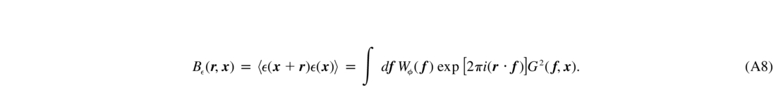
and the SF is readily obtained from the power spectrum using the Wiener‐Khinchin theorem
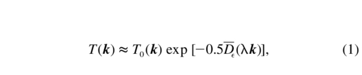
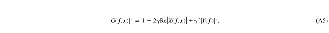
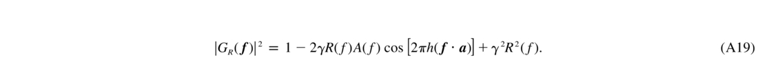
I call |G(f)|2 the "error transfer function" (ETF), because it describes the part of the atmospheric spectrum left uncorrected by the AO system. Low spatial frequencies (large‐scale perturbations) are usually well compensated for (G = 0), while high frequencies are not (Fig. 1). The general expression for the ETF is derived in the
Fig. 1.— ETFs at the center of the field for optimum GLAO with θ0 = 1 5 at several layer altitudes. For reference, θ0h = 0.44 m at h = 1 km.
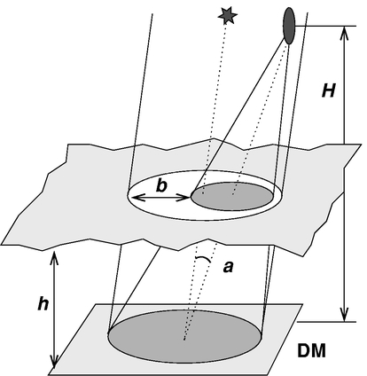
Fig. 2.— Geometry of ground‐layer sensing with LGS (see
In GLAO, the spatial scale of the compensation depends on the altitude; so does the ETF. The atmospheric turbulent volume can be represented by a combination of an arbitrary number of thin turbulent layers. The ETF is computed layer by layer. As the layers are statistically uncorrelated with each other, the resulting power spectrum W(f) is a sum of the power spectra of all layers. The von Kàrmàn phase power spectrum of ith turbulent layer is (Tatarskii 1971; Roddier 1981)
where r0,i is the Fried radius for layer i, r-5/30,i = 0.423(2π/λ)2Ji, and Ji = C2ndh is the turbulence integral for that layer, measured in m 1/3. The effect of outer scale turbulence L0 is included. The SF for the uncorrected turbulence with infinite outer scale is given by the familiar formula
where λ is the imaging wavelength, and J = ∑iJi is the total strength of the turbulence.
I take advantage of the fact that the turbulence strength Ji and the wavelength enter in equation (4) as multiplicative factors, and compute the "normalized" residual SFs Di(r) for each layer with r0,i = 1. Then the contribution of each layer is scaled by Ji and summed to get the final multilayer residual SF D as
where the normalized SFs (in m 5/3) are
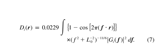
An additional term Dtilti(r) should be added to equation (7) to correct for the fact that with LGSs the tip‐tilt component of the wave front is measured on one or several NGSs, as detailed in the
The set of SFs Di depends on the geometry (layer altitudes, viewing directions, actuator pitch), but not on the TP. Thus, it makes sense to precompute Di and then to make their linear combinations, depending on TP and wavelength. This scheme is illustrated in Figure 3.
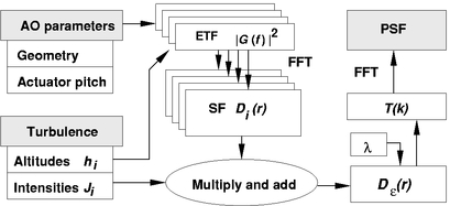
Fig. 3.— Block diagram of PSF calculation.
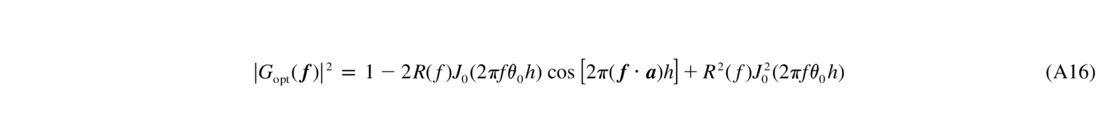
As an example, the ETF for the so‐called optimum filter (eq. [A16]) is
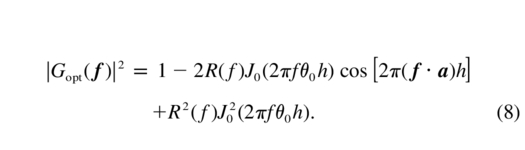
Here R(f) describes the smoothing due to deformable mirror (DM), which I model as a simple cutoff beyond the Nyquist frequency 1/(2d) for the projected actuator pitch d (e.g., Rigaut et al. 1998). For each layer at altitude h, the phase is smoothed over the length θ0h, where the parameter θ0 defines the size of the corrected field (Fig. 1). The angle a between the object and the center of the field enters through the cosine term and leads eventually to the angular asymmetry of the SF, OTF, and PSF, because all other terms in equation (A16) are rotationally symmetric. Near the center of the field, θ≪θ0 and the Bessel function J0(2πf θ0h) goes to zero well before the cosine term can produce any asymmetry. For θ>θ0, the situation is reversed and the PSF becomes asymmetric.
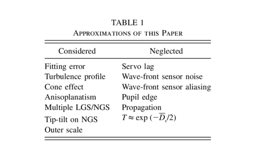
The analytical method outlined above is only approximate. So far, I ignore the temporal behavior of the AO system, assuming the correction to be instantaneous. The noise in the wave‐front sensor is also neglected. These additional factors increase the phase residuals. Thus, the analytical method gives an optimistic prediction of the PSF. The approximations made in this paper are listed in Table 1. Several comparisons of the analytically computed PSFs with direct Monte Carlo simulations have shown good agreement.
 |
It is implicitly assumed throughout this paper that the observations are done at zenith. For some zenith distance z, the altitudes should be replaced by hsec z, and the turbulence intensities Ji in equation (6) should be multiplied by sec z as well.
3. RESIDUAL STRUCTURE FUNCTION AND TURBULENCE PROFILE
The degree of turbulence compensation—GLAO gain—is the ratio of the uncompensated atmospheric SF Dϕ(r) to the residual SF D(r), where r = |r|. The gain depends on the altitude h: the low layers h<Hmin are compensated well, to a level set by the DM actuator spacing, and the high layers at h>Hmax are left uncorrected. The turbulence in the "gray zone" Hmin<h<Hmax is partially corrected. The parameters Hmin and Hmax loosely define the limits of this zone and are discussed below.
To get some insight into the GLAO gain, I consider the simple case of the optimal filter (eq. [A16]); i.e., averaging each layer over a cone with half‐angle θ0. A family of SFs normalized to r0 = 1 m is plotted in Figure 4 for θ0 = 15, a perfect DM (R[f] = 1), and infinite outer scale. For high layers, these SFs approach the uncorrected SF Dϕ(r) = 6.88(r/r0)5/3, so the GLAO gain is close to 1. For low layers, the residual SFs saturate, and the gain at large baselines is significant.
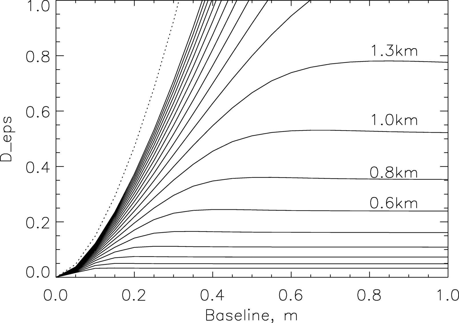
Fig. 4.— Normalized residual structure functions (eq. [7]) in m 5/3 for optimum GLAO (θ0 = 15) for layer altitudes hi = 200 m × 100.1i (0.2, 0.25, 0.3, ..., 15.9 km). Labels indicate some altitudes; the dotted line is 6.88r5/3.
There is a very simple analytical approximation of this family of residual SFs:
This formula has correct asymptotes in the limits r→∞ and r→0. It differs from the exact SFs by less than ±20% over the whole range of parameters and is useful for qualitative analysis.
The GLAO gain (denominator of eq. [9]) depends on the altitude and baseline r. Which baseline is the most representative one? Recall that the OTF is proportional to exp [-D(r)/2] (eq. [1]). At short baselines the OTF is very close to 1, at large baselines it is practically zero, so only a small range of baselines in which D(r)∼2 influences the PSF. For uncompensated turbulence, the full width at half‐maximum (FWHM) resolution is β = 0.98λ/r0 (Roddier 1981), and the SF is close to 2 at a baseline r∼r0/2 ≈ λ/(2β). Hence, if a GLAO system reaches some angular resolution β, the critical baseline will be of the order r∼λ/(2β).
According to equation (9), a GLAO gain of 2 at a critical baseline is reached at a layer of altitude Hmax∼λ/(β θ0). For higher layers, the GLAO gain is less than 2 (almost no compensation), whereas lower layers will be well compensated. The above estimate of Hmax is, of course, quite crude; it depends (through β) on the atmospheric conditions.
Eventually, the GLAO smoothing length 2 θ0h for low layers becomes smaller than the projected actuator spacing d. In this case, the compensation quality is limited by the DM resolution, as in classical AO. The calculations of Di with finite DM resolution confirm this statement: in a plot similar to Figure 4 but with d>0, there is no improvement in GLAO gain below Hmin = d/(2 θ0). Thus, Hmin is a reasonable estimate for the lower boundary of the "gray zone."
The analysis of the residual SF shows that for predicting GLAO PSF, it is necessary to know the integrated intensity of turbulence in the low layers h<Hmin, the integrated intensity of the high layers h>Hmax, and the detailed TP in the "gray zone" Hmin<h<Hmax. For example, for λ = 0.7 μm, θ0 = 15, and β = 0 2, the "gray zone" extends from 570 to 1600 m with respect to the conjugation altitude of the DM. If the DM is conjugated to ∼150 m below ground, as in a large Cassegrain telescope with a deformable secondary mirror, the effect of this mismatch will be small. However, when a higher compensation order (smaller d) or a wider field are wanted, the same mismatch may be intolerable, because it will seriously affect the GLAO gain.
For GLAO, we need to know the detailed TP in the first kilometer above the observatory. This is a new requirement since, for example, a classical AO is most affected by the highest and fastest layers. For accurate GLAO modeling, the vertical resolution of the TP should be of the order of Hmin or better. However, this resolution is relevant only below Hmax, because higher layers remain essentially uncorrected, and all we need to know is their integrated intensity.
4. PERFORMANCE OF GLAO
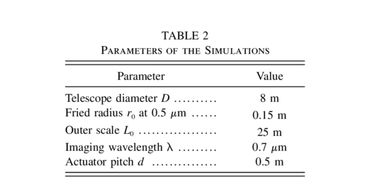
The method outlined above is illustrated with several examples. The parameters that are common to all examples are listed in Table 2. The atmospheric conditions correspond to a median seeing at good sites with a 0495 FWHM of the uncorrected atmospheric PSF at 0.7 μm (see Tokovinin [2002] for the FWHM computation with outer scale). The vertical distribution of turbulence (TP) is varied to evaluate its effect on the GLAO performance.
 |
Different wave‐front sensing schemes are compared. An S‐GLAO system averages signals from five sodium LGSs at 90 km altitude, arranged in a regular pentagon with a 2' radius. This configuration approximates the ring‐shaped beacon required for optimum GLAO. A single Rayleigh LGS at 10 km (R‐GLAO) is studied for comparison. While the first system approximates the optimum filter, the R‐GLAO is a more economical and robust option. The contributions from tip‐tilt sensing on natural guide stars Dtilt are neglected in both cases.
- The "Gray Zone."—For a GLAO system with the optimum filter (eq. [A16]), I show in Figure 5 the dependence of the width of the corrected PSF on the altitude of the low layer. In this example, 20% of turbulence is placed at a fixed altitude of 10 km; the remaining 80% is in a thin layer with variable altitude. Other conditions are described in Table 2. This figure illustrates the transition from a well‐corrected ground layer at h<0.5 km to almost uncorrected turbulence at h>1.5 km, in agreement with the crude estimates of § 3. When the bulk of the turbulence is concentrated in the "gray zone," even the optimum GLAO gives a PSF that is nonuniform over the field and is elongated. In such conditions, GLAO should work with a reduced field size. The Cerro Pachón seven‐layer TP model used extensively in modern AO studies (Chun 2003) does not contain any layers in the gray zone, so it should not be used for predicting GLAO performance.
- The Field‐Resolution Trade‐off.—This is illustrated in Figure 6, where the energy concentration and FWHM are presented for two choices of the field radius θ0. The TP selected for this example consists of four layers at 0, 0.2, 0.5, and 8 km, with fractional strengths of 0.4, 0.3, 0.1, and 0.2, respectively, and models an extended turbulence distribution near the ground. The difference in the optimum GLAO performance resulting from opening the cone angle from θ0 = 2' to θ0 = 4' is clearly seen: the uniformly corrected field is wider, but the resolution is worse. In both cases, the PSF is quite isoplanatic inside the θ0 cone.The optimum GLAO filter (eq. [A16]) corresponds to wave‐front averaging on a ring of radius θ0h. It is shown by Tokovinin et al. (2000) that this choice leads to the best possible correction at the edge of the field (indeed, note in Fig. 5 that the PSF at the edge can be narrower than at the center). It turns out that this prescription also leads to a very uniform correction over the whole field. On the other hand, if the wave fronts are averaged over the circular region of radius θ0h as proposed in Jolissaint et al. (2004), the uniformity is worse (dotted lines in Fig. 6). Averaging over a circle (as opposed to a ring) gives more weight to the center of the field, so the correction at the center improves at the expense of the correction at the edge.
- The Dependence on TP.—Three representative TPs are modeled. All have 17% of the turbulent energy in a layer at 8 km, essentially uncorrected, while 83% is concentrated in a layer either on the ground (good TP), at 0.5 km (medium TP), or at 1 km (bad TP). If the ground layer were corrected perfectly, the residual seeing would be 0.173/5 × 05 = 017. The influence of the TP on the S‐GLAO performance is shown in Figure 7. The correction is excellent and uniform for a good TP, as expected. The PSF asymmetry is greatest for the medium TP and improves again for the bad TP, because the correction is uniformly poor.Figure 8 compares the S‐GLAO with the R‐GLAO. The first system gives a more uniform correction over a range of conditions. At the edge of the field (2'), the correction for a good TP is better than at the center, because the object coincides with one of the LGSs. The R‐GLAO has worse PSF uniformity, but better on‐axis resolution.
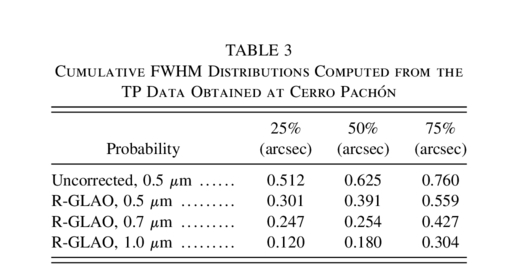
- Statistics of the Performance.—The ability of the analytical method to process a large number of TPs is essential for the statistical prediction of the GLAO performance. For example, Figure 9 plots the distributions of the FWHM resolution that are expected from an R‐GLAO system working at Cerro Pachón in Chile. A total of 4233 low‐resolution TPs were measured in 2003 January over 21 nights. A similar plot was given in Tokovinin (2004). However, the data are reprocessed here with some important changes. The intensity of the lowest (ground) layer is reduced by a factor of 2 compared to the actual data to compensate for the site‐testing instrument being located too close to the ground (1.5 m, as opposed to ∼20 m for a typical telescope dome height). The turbulence outer scale is also taken into consideration. Thus, the median size of the uncorrected PSF at 0.5 μm is 063, which is typical for good sites. Compared to the earlier estimate, the resolution gain of GLAO is somewhat reduced, but it is still highly significant. The levels of the cumulative distribution are listed in Table 3. The GLAO improves the resolution more than 75% of the time. The best image quality in the red part of the spectrum approaches 01, opening a new perspective for ground‐based astronomy in its competition with space.
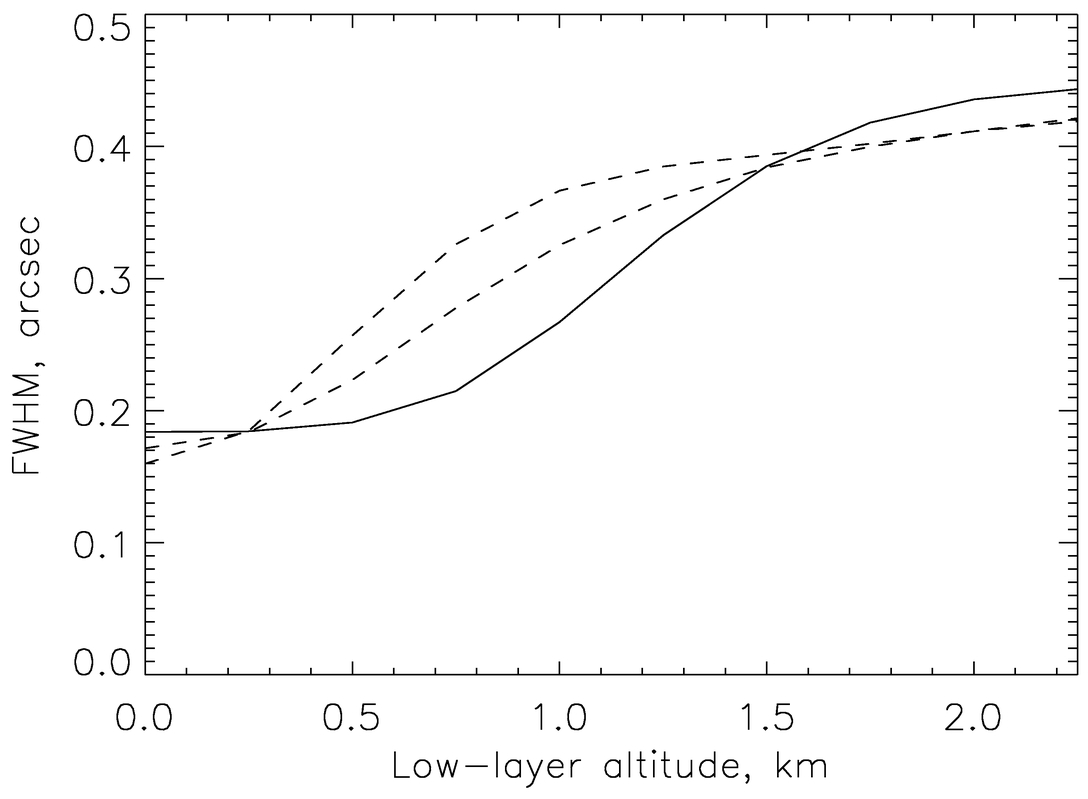
Fig. 5.— FWHM of the GLAO‐compensated PSF in two orthogonal directions at the center of the field (solid line) and at 15 offset (dashed lines) for the optimum GLAO system (θ0 = 15) as a function of the low‐layer altitude. Imaging wavelength is 0.7 μm, uncorrected FWHM is 0495.
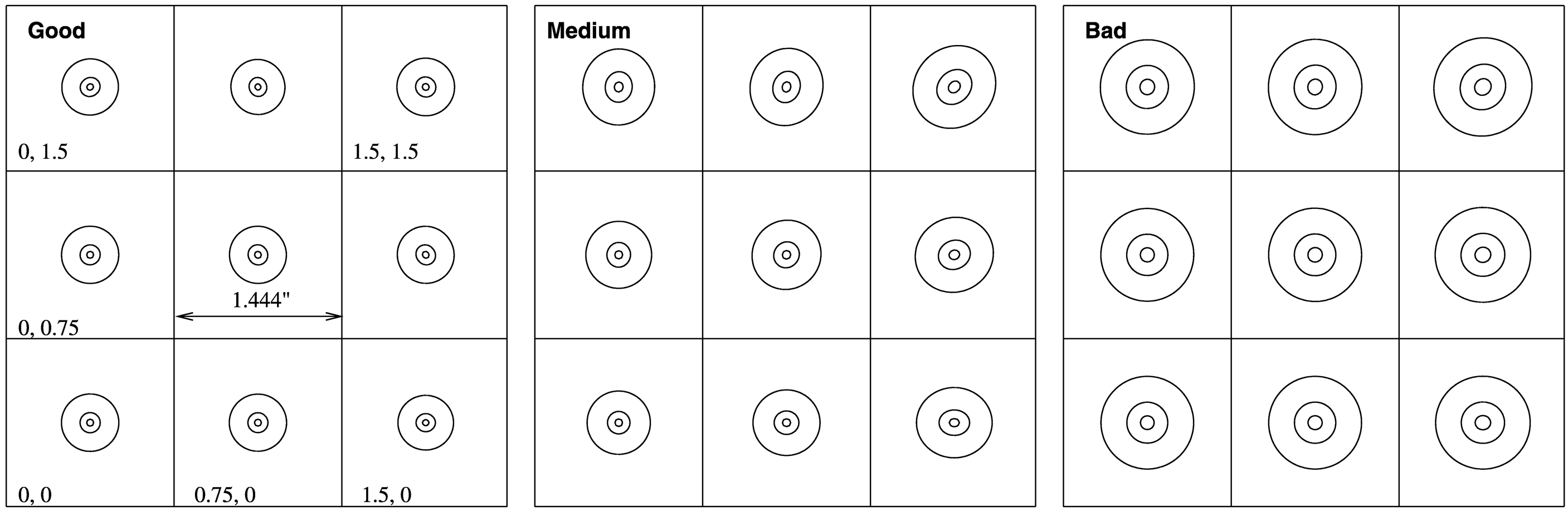
Fig. 7.— Mosaic of PSF contours (at 0.1, 0.5, 0.9 levels) in the field of view for the S‐GLAO system. Each box is 1444 on a side, the center is in the lower left corner, and other boxes are placed at 075 step. Left to right: good, medium, and bad turbulence profiles.
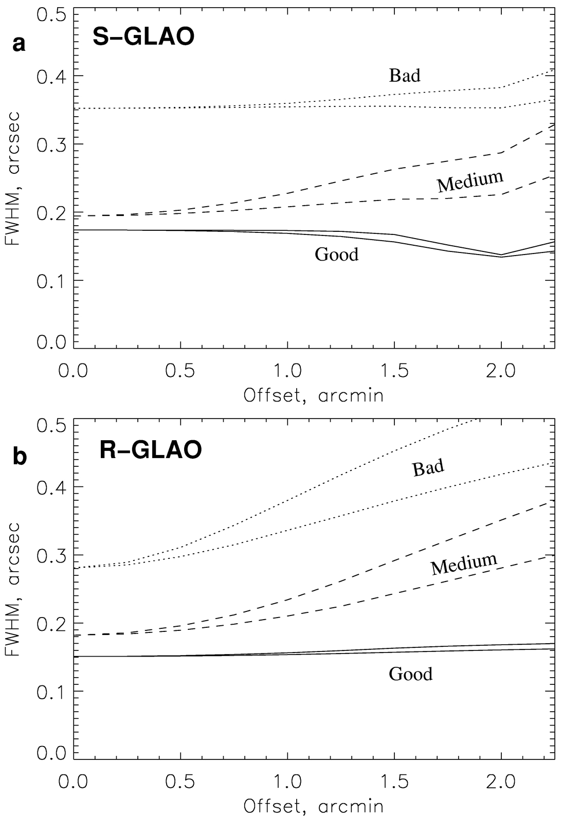
Fig. 8.— FWHM of compensated PSF across the field for S‐GLAO (a) and R‐GLAO (b). The FWHM in two directions are plotted to evaluate the ellipticity of the PSF. Solid, dashed, and dotted lines indicate good, medium, and bad TPs, respectively.
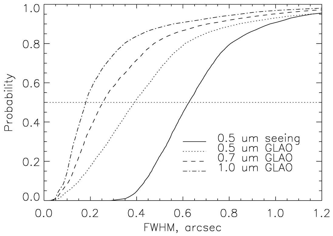
Fig. 9.— Cumulative distributions of the uncorrected seeing‐limited FWHM and the on‐axis FWHM at three imaging wavelengths corrected by R‐GLAO, based on Cerro Pachón turbulence data.
 |
5. CONCLUSIONS
The analytical method of evaluating the PSF developed here for GLAO allows us to understand the influence of various parameters on the final performance metrics—resolution, energy concentration, and PSF uniformity. The major conclusions are as follows:
- 1.Depending on the desired size of the corrected field θ0 and the achieved resolution β, the upper boundary of the corrected "ground layer" is of the order of Hmax∼λ/(β θ0).
- 2.All turbulent layers below Hmin = d/(2 θ0) are corrected equally well and are limited by the projected actuator spacing d.
- 3.The turbulence in the "gray zone" between Hmin and Hmax is partially corrected; it causes most of the residual anisoplanatism and PSF asymmetry. When the gray zone is turbulent, GLAO corrects a reduced field of view.
- 4.In order to predict GLAO performance and to operate efficiently, a knowledge of the turbulence profile with a resolution of Hmin or better is needed. Layers above Hmax do not have to be measured at a high resolution, because only their integrated strength matters.
- 5.For an 8 m telescope with good seeing, a single Rayleigh LGS is sufficient for ground‐layer sensing. Compared to the optimum array of sodium LGSs, it gives better on‐axis correction but worse PSF uniformity over the field when the turbulence profile is "uncooperative."
Comments by B. Gregory are very much appreciated; they helped to improve the presentation. The author is indebted to the anonymous referee for the detailed analysis of the formulas, and other valuable comments.
APPENDIX: DERIVATION OF THE SPATIAL FILTER
I derive here a general expression for the GLAO error transfer function and give its specific forms for some cases of interest. I neglect wave propagation effects and use geometric optics.
A1. HEURISTIC FILTER
A GLAO system with a LGS is illustrated in Figure 2. I consider only one thin turbulent layer at altitude h above the DM conjugation level, called "ground" for simplicity. The beacon's altitude is H. The angular distance between the beacon and the object changes across the telescope pupil. Let a be the beacon‐object angle as viewed from the center of the aperture, and x the coordinate vector in the aperture plane. The beacon (or the center of multi‐LGS array) is assumed to be located on the optical axis of the telescope. From simple geometry, the relative shift b between object and beacon wave fronts viewed from the point x in the aperture (Fig. 2) is
The beam from the object at infinity is cylindrical, whereas the LGS beam is conical. Because of this, the diameter of the turbulent layer sampled by the beacon is γ = 1 - h/H times smaller than that sampled by the object. The factor γ between the spatial scales of LGS‐sensed and object wave fronts precludes straightforward use of Fourier techniques. This barrier can be circumvented by a heuristic argument that the aberrations as sensed by LGS are reduced γ times with respect to the aberrations from the object (wave‐front slopes measured by a Shack‐Hartmann sensor are indeed reduced by a factor γ). I follow this heuristic reasoning, which replaces spatial "stretching" by the reduced amplitude of the compensating phase, and come back to a more accurate derivation below.
The compensating phase is derived by shifting the atmospheric phase by b and smoothing by convolution with the spatial response of the DM. Additional smoothing will occur if the signals from multiple laser beacons are averaged. To cover this case, I introduce the "beacon shape" factor, which describes the angular distribution of the beacons on the sky. The corresponding spatial filter is
where the low‐pass spatial filter R(f) describes the finite resolution of the DM, while the FT of the angular intensity distribution of multiple beacons S(k) is normalized to S(0) = 1. A single LGS is represented by a point source (S = 1). The filter X depends on the position in the pupil x through the displacement b :
In the heuristic approach, the residual phase (x) is the difference of the original phase and the γ‐scaled correction. The FT of the residual phase is the product of the atmospheric phase and the spatial filter G:
The filter that relates the residual power spectrum to the atmospheric power spectrum (ETF) is
where Re stands for the real part of the complex number. I take equation (A3), which shows the dependence on x , and average over x within the telescope aperture—a circle of diameter D. The averaging leads to the Airy function
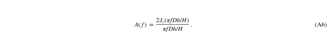
The aperture‐averaged heuristic filter is, finally,
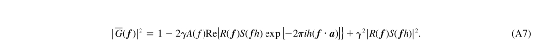
For turbulent layers lying above the laser beacon (h>H), we have to set γ = 0, which means no turbulence compensation.
A2. EXACT FILTER
A slightly more complex formula for the filter results if the stretching is explicitly taken into account. I want to compute the ETF by evaluating the covariance function of the residual phase and representing it as a spectral integral of the Wiener‐Khinchin theorem (the angular brackets denote ensemble average):
The phase residual is written formally as a Fourier integral
where ϕ˜(f) is the FT of the atmospheric phase. I formally compute the covariance as a product of two Fourier integrals (eq. [A9]) over spatial frequencies f and f', reduce it to the double integral, and take advantage of the fact that 〈ϕ˜(f)ϕ˜*(f')〉 = Wϕ(f)δ(f - f'):
Given the dependence of X on the coordinate x in equation (A3), I obtain

The following transformation will be correct for the Kolmogorov power‐law phase spectrum, and approximately correct for the von Kàrmàn spectrum at high spatial frequencies:
Using this result, I take the expression in equation (A8) for B(r,x), consider each term of equation (A12) separately, and, where necessary, rescale the e2πiγ(r·f) terms to convert them into e2πi(r·f). The resulting G2 is complex, but the correlation function B in equation (A8) is real, because the phase power spectrum is symmetric over f
, and X(f) is a Hermitian, X(- f) = X*(f). Hence, G2 is also Hermitian. I can neglect the imaginary part of G2 and write the ETF as
to replace the heuristic formula in equation (A5). The averaging of |G|2 over the pupil leads finally to

where Y(f) is given in equation (A3).
I compared the heuristic filter given in equation (A7) with the more accurate expression in equation (A15). Most of the difference occurs at low spatial frequencies, where a heuristic filter has nonzero values, whereas the exact filter is always zero. However, for a Rayleigh LGS at 10 km, the residual SFs D match within 12%, and the use of a simpler heuristic filter is well justified. Needless to say, in the case of γ = 1 (low layers or NGS), both filters are equal.
A3. SPECIFIC CASES
Optimum Filter.—It has been shown analytically that the best correction of objects lying over a circle of radius θ0 is achieved by averaging the compensating phase over the circle of radius θ0h (Tokovinin et al. 2000). Such averaging corresponds to a cone with opening angle θ0 and can be done with a very large number of NGSs located on a ring. The corresponding FT of the beacon is S(k) = J0(2π θ0k), where J0 is the zero‐order Bessel function. Hence, the ETF is
When the wave fronts are averaged over the whole circular field, the beacon shape is S(k) = J1(2π θ0k)/(π θ0k) (Jolissaint et al. 2004). With such an ETF, the correction is less uniform over the field (Fig. 6).
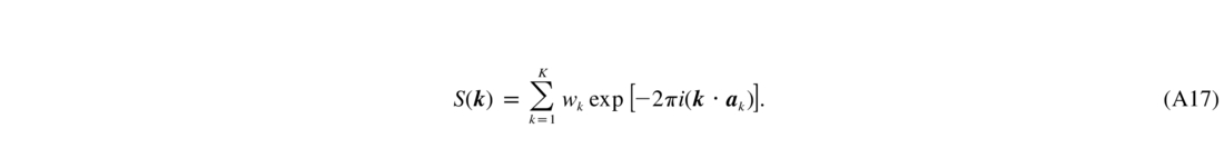
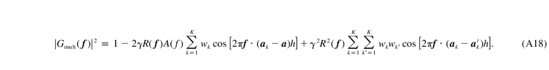
Multiple Beacons.—Suppose that we have K guide stars located at ak on the sky. Suppose that their signals are combined with weights wk, normalized so that ∑wk = 1. Then
Putting this in the heuristic filter (eq. [A7]) leads to
A large number of beacons uniformly distributed on a circle of radius θ0 approximates the cone required for optimum filtering. Regular rings of bright stars are not found on the sky, but rings of sodium LGSs (like S‐GLAO in § 4) are an excellent substitute, even for large telescopes.
Single Rayleigh Beacon.—The specific case of a heuristic filter for a single low‐altitude beacon is
Here, the selective compensation of low layers is possible, because of the factor γ and because of the aperture averaging A(f).
A4. TIP‐TILT COMPENSATION WITH NGS
Compensation of tip and tilt (t/t) is automatically included in the filter functions. However, with LGS the t/t signal is derived not from the beacon itself, but from additional natural guide stars. This substitution of the t/t signal leads to some modification of the residual SF.
The residual phase can be expanded on the Zernike basis with coefficients ei. As shown by Véran et al. (1997), the aperture‐averaged SF is then
with Uj,k being the cross‐correlations of Zernike modes averaged over aperture, and Ej,k the covariance matrix of the Zernike coefficients, Ej,k = 〈ejek〉. Of interest here are only Zernike modes 2 and 3. The corresponding correlation functions are U2,2 = 16(x/D)2, U3,3 = 16(y/D)2, and U2,3 = U3,2 = 16xy/D2, where r = (x,y).
Both the t/t coefficients e2 and e3 and their covariances Ej,k are modified by the substitution of the LGS tilt with the NGS tilt. For one turbulent layer i, the correction to the SF is thus
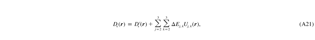
where ΔEj,k are the changes of the t/t covariances, and D'(r) is the SF calculated from the ETF given above.
Let tj be the tip or tilt coefficient for the observed object (target), bj the coefficient for the laser beacon, and gj the weighted coefficient for several NGSs. The coefficient of phase residual ej changes from tj - bj to tj - gj. The corresponding change of the covariance is

To compute ΔE, one needs to know the second moments (covariances) of Zernike coefficients for the target, LGS, and NGSs. The formula is provided by Whiteley et al. (1998) in their equation (27) as a one‐dimensional integral over spatial frequency (I do not reproduce this long formula here). I compute the covariances for one layer and for D/r0 = 1 normalization (they are equal to the Noll coefficients for two sources at infinity and for pure Kolmogorov turbulence). The layers above the LGS produce zero covariance. With normalized covariances E = (D/r0)5/3E', the correction for t/t to be used in equation (7) is

If t/t compensation is successful, the coefficients ΔE' are negative, because tilt residuals for NGS combination are less than for the LGS beacon. Thus, Dtilt is negative—its contribution diminishes the D—increasing the OTF and leading to a sharper PSF.
An ad hoc coefficient of 0.87 was introduced in equation (A23) to diminish the Dtilt. Without this coefficient, the residual SF becomes negative at baselines approaching the telescope diameter. The reason is for the large‐telescope approximation and other approximations made in the analytic PSF calculation. I checked that the coefficient 0.87 solves the problem and reproduces the classical results on resolution gain with t/t compensation: for infinite outer scale, a maximum Strehl gain of 3.7 at D/r0 ≈ 3 is obtained.
The method of accounting for t/t outlined here is only approximate. It works well for a single LGS, but in the case of multiple LGSs and NGSs, we need to compute all cross‐covariances, their numbers increasing as the square of the total number of sources. There is probably a better technique based on a direct filtering in Fourier space. For this reason, the t/t compensation was ignored in the examples presented above.