

ABSTRACT
The Planet Search Survey Telescope is an automated small‐aperture CCD imaging photometer designed to search for transits by extrasolar planets across the disks of their parent stars. It simultaneously observes thousands of stars with apparent R magnitudes between 10 and 13 in a field approximately 6° × 6°. Stars in this brightness range are well within the capability of the high‐precision radial velocity systems that have successfully detected over 100 extrasolar planets to date. The combination of the photometric transit depth and radial velocity amplitude can provide both the radius of the planet and a good estimate of its mass, since the orbit is nearly edge‐on. As a result, estimates of the planet's density and other parameters can be obtained.
Export citation and abstract BibTeX RIS
1. INTRODUCTION
Radial velocity observations have shown that extrasolar planetary systems with giant planets orbiting their parent stars are quite common (Mayor & Queloz 1995; Marcy & Butler 1996; Butler & Marcy 1996; Butler et al. 1997; Cochran et al. 1997; Marcy et al. 1997; Noyes et al. 1997; and in retrospect, Latham et al. 1989). Subsequently, the pace and breadth of work has increased (e.g., Butler et al. 2000, 2004; Gilliland et al. 2000; Tinney et al. 2001), and the first transiting giant inner planet was discovered orbiting HD 209458 (Charbonneau et al. 2000; Henry et al. 2000). Radial velocity observations can only provide a lower limit on the planetary mass, because of the unknown orbital inclination. If a planet's orbital plane is aligned nearly along our line of sight, the planet will pass between an Earth‐based observer and its parent star, an event known as a transit. The uncertainty in the planetary mass derived from radial velocity observations is greatly reduced when the orbit is nearly edge‐on. The transit also provides an estimate of the projected area of the planet, thus allowing its radius, and therefore also its density, to be estimated. The case of HD 209458 has shown that this is possible in practice. The brightness of this star also allowed detailed work to be done to further elucidate the nature of the planet (Brown et al. 2001, 2002; Charbonneau et al. 2002). Work of this nature is less rewarding for transiting systems involving fainter stars, such as OGLE‐TR 56 (Konacki et al. 2003) and OGLE‐TR 113 (Bouchy et al. 2004).
Calculations of the expected detection rates for short‐period transiting planets (Brown 2003) suggest that ∼104 stars monitored with a 2% or better precision over 2 months will yield one to two transiting planets. The number of stars of sufficient brightness available to a given system depends primarily on the product of the telescope's collecting area and the solid angle on the sky of its associated focal plane detector system. For a given detector size and system f‐ratio, a larger telescope will cover a smaller field over a fainter useful magnitude interval (with correspondingly more stars) than a smaller telescope. There is a weak improvement in the trade‐off between field of view and star counts (Cox 2000) as the telescope aperture increases. We have opted in favor of the small telescope and wide‐field approach primarily because the bright stars in our useful magnitude range are within the observing capability of the high‐resolution radial velocity instruments. Additional follow‐up observations, such as those already done in the case of HD 209458, are also more rewarding for brighter stars than for fainter ones. Finally, small systems are relatively inexpensive, so it is possible to build several of them operating at different longitudes. This increases the light curve coverage in a given observing season by effectively increasing the length of the night, and also by improving the weather statistics. Those lines of reasoning have led to the development of a number of wide‐field, small‐aperture transit search programs, including those of our collaborators (STARE1 and Sleuth2) and others (Borucki et al. 2001; Horne 2003; Bakos et al. 2004).
The number of stars in a given field also depends on the Galactic latitude, but there is a trade‐off to be made between the number of target stars in the field and the number of false alarms produced by astrophysical effects other than planetary transits (Brown 2003). A magnitude‐limited image of a richer field near the Galactic plane tends to include more distant giants than a similar field at a higher latitude. This results in more false alarms due to eclipsing binaries with shallow eclipses. In addition, a crowded, low‐latitude field, combined with a small system's coarse pixel scale on the sky, will result in numerous blends of bright target stars with faint background eclipsing binaries. Obviously, a low‐latitude field will have more extrasolar planetary systems in it than a high‐latitude field, but the amount of follow‐up work required to weed out the false alarms is higher for the low‐latitude fields. Follow‐up observations are a critical component of a complete transit search program, but a discussion of them is outside of the scope of this paper.
The giant inner planet models of Guillot et al. (1996) and Burrows et al. (2000) indicate that the radii of these objects depend only weakly on their mass in the range of 0.5MJup–3MJup. Radii range from approximately 0.5RJup to about 1.2RJup, depending on composition. Thus, we expect a transit depth on the order of 0.25% to 2.0%, depending on planetary composition and stellar size. This expectation was borne out by the observed transits of HD 209458, which are 1.6% deep, and OGLE‐TR 56, with a transit depth of 1.2%. The duration of a transit is approximately 2.5–3 hr for objects with periods of ∼4 days and orbital radii of ∼0.05 AU. Thus, to detect a transit reliably (i.e., with 7 σ confidence), we need to achieve a differential signal‐to‐noise ratio (S/N) of 0.5% or better in an integration time of ∼30 minutes. It is important to realize that only differential precision of one star's light curve compared to other stars in the field over the duration of a transit is required. There is no requirement for correction to a standard photometric system, all‐sky photometry, use of standard stars in other fields, etc. One weakness of the wide‐field, small‐aperture approach to transit searches, however, is that the photometry is more affected by differential extinction across the field, making it more difficult to achieve the requisite differential photometric precision. Scintillation is also a significant noise source for a small system (Dravins et al. 1998) and can be the dominant contributor for the brightest stars.
It is obviously important to operate the system as much as the weather and diurnal cycle will permit. The cost to support an observer for such a massive and tedious observing program could be prohibitive, but the simplicity of the observing procedure lends itself to an automated observing approach. We have therefore developed the Planet Search Survey Telescope (PSST) as an automated observing system.
2. SYSTEM DESCRIPTION
The considerations of § 1 provide the basic requirements for the PSST system. It is a wide‐field, small‐aperture CCD imaging photometer capable of obtaining precise differential photometry on thousands of stars simultaneously, and it is operated in an automated manner. The details of the system implementation are described in this section.
2.1. Hardware
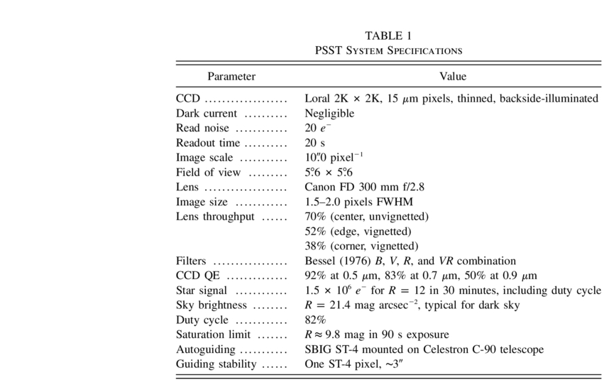
The PSST detector is a 2K × 2K thinned, back‐illuminated Loral CCD with 15 μm pixels processed at the University of Arizona CCD lab. It has excellent quantum efficiency and good cosmetics. It is operated by a Gen II Leach controller from Astronomical Research Cameras, Inc. (Leach et al. 1998). The CCD is read out at about 200 KHz, and its read noise of about 20 e− is less than the shot noise of the sky on a moonless night. Cooling is provided by a CryoTiger cryocooler system. This is a compressor‐based cooling system similar to a kitchen freezer, using the expansion of the proprietary refrigerant in the cold head to achieve low temperatures. There is essentially no vibration at the cold head, since the system lacks the expansion piston found in helium‐based cryocoolers. The cold head runs between −170°C and −190°C, depending on the outside temperature, cooling the CCD to its regulated operating temperature of about −110°C. We initially operated the CryoTiger compressor in the same enclosure as the computers (see below) but then moved it out on the observing floor. The compressor works well in cold winter temperatures in Flagstaff, but it tended to overheat in the summer when it was located in the computer enclosure.
The optical system consists of a Canon FD 300 mm, f/2.8 sports photography lens and Johnson B, V, and Kron‐Cousins R filters, in addition to a combined VR filter (Bessel 1976). The Canon lens forms images with a FWHM of ∼1.6 pixels at a plate scale of 10 0 pixel−1, but it vignettes by up to 60% in the corners of the field. The throughput of the lens in the field center is about 70%. There is a small residual tilt between the focal plane of the lens and the CCD surface, which causes the PSF to vary slightly across the field. This has been annoying, but not yet sufficiently troublesome to warrant being fixed. We normally observe with the R filter. Initially, we used the VR filter, but the benefit of the additional flux obtained was outweighed by the difficulty in obtaining a good color correction with such a broad passband. On several nights throughout the season, we also obtain B and V exposures that are used to estimate stellar colors.
Flat fields are obtained by pointing the telescope to a north‐facing white screen that is illuminated by the twilight sky. This setup was found by Chromey & Hasselbacher (1996) to be well suited for very wide fields of view.
The guider consists of an SBIG ST‐4 autoguider mounted on a C‐90 telescope that is firmly attached to the structure of the instrument mount. The residual differential flexure between the guider and the main camera is corrected after each frame using the science data. A key improvement in the guiding occurred when we incorporated code (Timothy Brown, 2001, private communication) to update the ST‐4's target tracking location after each image. The guider can operate with stars as faint as about 6th magnitude, and it provides guiding stability of about one‐third of a pixel on the science CCD.
The lens and its focus stage, filter wheel, shutter, CCD Dewar and CryoTiger cold end, CCD controller, and the C‐90 with the ST‐4 are all mounted on a common structure supported between the fork arms of a mount taken from a Celestron Compustar C‐14 telescope (see Fig. 1). The telescope control electronics were built at Lowell Observatory using a PC‐based commercial stepping motor controller board and motor drive units. Limit and home switches were added to the mount for right ascension and declination, and to the support plate for focus. The mechanical alignment of the declination bearings in the fork arms was inadequate for proper operation over the full range of declination, causing the telescope to bind at certain positions. The mount was modified and pinned in place in the Lowell Observatory shop and now operates smoothly everywhere in the sky.
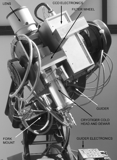
Fig. 1.— Photograph of the Planet Search Survey Telescope at Lowell Observatory. The principal components of the telescope are labeled.
The Sun SPARC Ultra 5 camera control computer and the industrial PC telescope control computer are mounted in an insulated, temperature‐controlled enclosure. The enclosure keeps them at a reasonable operating temperature and protects them against possible water damage in case of a serious system failure. Power and network connectivity are derived from the control building in the 31 inch (78 cm) telescope enclosure at Anderson Mesa.
A simple but very helpful addition was a four‐channel computer‐controlled AC power distribution unit (it should be noted that commercial products with more capability than this homemade device are now available). This device was made from four solid‐state relays and is controlled by the parallel port of a Sun SPARC Ultra 5 computer. Each solid‐state relay is connected to adjacent bits in the parallel port, so that the relays are all off when the computer is rebooted. This causes all the power to be off if the computer reboots, a safe state for the system. The four channels are individually addressable, allowing the power of various components to be cycled by the observing script. This capability is used to recover from several types of hardware and software failures. In hot summer weather, the script powers off everything except the Sun computer, but in cold weather, power remains on during the day.
2.2. Control Software
The PSST control software is the Lowell Observatory Instrument System (LOIS; Taylor et al. 2000, 2004). It is a modular instrument control software system based in part on Tcl/Tk. The LOIS package now controls most of the instrumentation at Lowell Observatory, in addition to the test‐bed system for the Kepler mission (Koch et al. 2000), the MagIC camera for the Magellan telescopes, and HIPO, an instrument for SOFIA (Dunham et al. 2004). Because it uses Tcl/Tk, the scripting features of that language are immediately available for use in LOIS. The telescope control system is the MOVE software package developed over the years at Lowell Observatory by Larry Wasserman. In the process of modifying the MOVE code to deal with the PSST‐specific hardware, its start‐up activities were made noninteractive. LOIS controls MOVE through a serial interface connection, thus being able to control the entire system in a coordinated manner.
The PSST control scripts are quite complex and can handle normal observing procedures and a number of abnormal situations. Normal observing commences when the PSST receives an e‐mail asking it to observe. We have two scripts: one for normal observing in the R band only, and another for obtaining multicolor observations. The system is then powered up, the telescope initializes its coordinates, and when the Sun elevation reaches a set angle below the horizon, the roll‐off roof is opened and the telescope slews to point at the flat screen. Test exposures are taken until the illumination level reaches a predefined value, and then flat fields are taken (either in three filters or only in the R band, depending on the script). The system waits until the field is high enough to start observing, then takes bias frames and automatically acquires the field and focuses the lens. An offset is made to compensate for the normal focus drift during the night as the temperature drops. Finally, the autoguider is enabled and observing commences. All R‐band exposures are 90 s long and are taken as rapidly as possible, achieving a cadence of less than 2 minutes. The design of LOIS allows a given exposure to be overlapped with storage and real‐time analysis of the previous image so that the dead time between frames is largely the CCD readout time. Images are obtained until either the field is too low in the west or the Sun is getting too high in the east. The dome is closed when one of these conditions is met, the telescope is sent home, and data compression and FTP transmission to the computers at Mars Hill begins. Generally, when we arrive at work in the morning, the night's data set (200–300 exposures) is ready for analysis.
The control scripts can handle some off‐nominal conditions autonomously. For example, the system can manage to work around partly cloudy conditions, crashes of the telescope control computer, and loss of track. Other conditions are less common and also more difficult to handle. The scripts handle these by putting the telescope in a safe condition and sending a text message to our cell phones, with a description of the problem in the subject line. Manual interaction with the system over the network can almost always correct the problem. We have not made any attempt to make the system aware of the weather, choosing instead to rely on the judgment of a person in Flagstaff to determine whether the e‐mail for starting the system should be sent or not.
Several files are generated during the night for the purpose of tracking the instrument's performance in real time, if needed, and assessing the quality of the night's data the next morning. These include guiding errors (both in the science CCD and the guider), guide star brightness, focus position, CryoTiger cold tip and CCD temperatures, image FWHM, sky brightness, and brightness and position of 10 photometric check stars. A single graphic summarizing the diagnostic information from these files is generated in the morning so that it is easy to catch any problems early and determine the quality of the night's data at a glance. In addition, LOIS produces an observing log file with general information about each image obtained that night.
3. DATA PROCESSING AND ANALYSIS
3.1. STARE Photometry
For the first several years of the PSST operation, analysis was performed with the STARE data analysis package provided by Tim Brown. This analysis package is a processing pipeline implementation of the weighted aperture photometry approach. A master star list for each field is constructed by co‐adding a number of frames taken on one or more photometric nights and performing aperture photometry using DAOPHOT II (Stetson 1987). The coordinates and magnitudes in the master star list are then tied to the Tycho‐2 catalog (Høg et al. 2000), and these data are used as a positional and photometric reference for the subsequent steps. The pipeline begins with the usual calibration steps: bias and overscan subtraction, and flat fielding. After that, a weighted‐aperture photometry is carried out, followed by extinction correction, including a linear color‐dependent term and a low‐order polynomial term to allow for positional dependence of the extinction across the field. This allows good measurements to be obtained in the presence of light cirrus, and it significantly increases the amount of useful data. The pipeline ends with the construction of the nightly time series and the removal of correlated frame‐to‐frame offsets.
Within the STARE package, we used two different schemes for weighting the pixels in the photometric apertures. The initial approach, which we ultimately returned to, is the traditional S/N‐weighting based on the calculable random noise from the star, sky, and detector. We also tried the optimal pixel weighting scheme described by Jenkins et al. (2000). This produced slightly better results than the S/N‐weighted approach, but the weights had unintuitive behavior, and the parameters needed to be determined with considerable care. Removal of the frame‐to‐frame variations was done using a single‐value decomposition (SVD) scheme. With proper selection of parameters, the variations between frames could be removed without also removing transit signals in the light curve.
3.2. Difference Image Analysis (DIA)
Our current data analysis pipeline is based on the optimal image subtraction approach described in Alard & Lupton (1998) and Alard (2000). We use the image interpolation and subtraction routines from the ISIS 2.1 package kindly made available by Christophe Alard,3 while the code for the remaining steps (star finding, geometric transformations, photometry of the difference images and transit search) was developed by us. This analysis pipeline was made practical by the availability of inexpensive but fast PC computers running the Linux operating system. We purchased three of these systems, and they have made a fundamental improvement in our data analysis capability.
3.2.1. Image Preparation
All images are trimmed, overscan and bias‐subtracted, and flat‐fielded using the appropriate tasks in the IRAF4 package (Tody 1993). After subtraction of the bias measured from the overscan region, the images are further corrected by subtracting a two‐dimensional bias pattern obtained from the average of 20 zero exposure time (bias) frames taken before and after the program exposures on every night. The flats are prepared from the nightly averages of 10 high‐S/N exposures of the flat‐field screen.
The next step in the pipeline is the rejection of low‐quality exposures (taken through cirrus or contaminated by bright airplane trails, meteors, etc.) and masking of the saturated pixels. Because of the strong vignetting in the optical system (more than 50% at the edges of the image; see Table 1) adopting a constant saturation level for the entire flat‐fielded image will reject many bright stars near the edges that are not in fact saturated. Instead, we prepare a saturation cutoff image IC, which is used to mask the saturated pixels as follows. A quadratic surface is fitted to one of the nightly R flats, and every pixel of IC is set to the value of the fitting function at the coordinates of the pixel. The reciprocal of IC is then normalized so that its central value is equal to saturation level at the center of our images. The result is an image in which each pixel has a value approximately equal to the value of the saturation cutoff at that pixel. It is then very easy to mask the saturated pixels in any program frame by marking all pixels whose value exceeds the value of the corresponding pixels in the cutoff image IC.
 |
3.2.2. Image Resampling and Subtraction
Before the kernel fitting and image subtraction can proceed, all images must be resampled to a common pixel grid. One of the exposures taken at a low air mass on a moonless photometric night is chosen as the reference frame for the field, and profile‐fitting (PSF) photometry is carried out in that image using Peter Stetson's DAOPHOT II/ALLSTAR suite (Stetson 1987, 1992). The PSF photometry has the advantage of producing accurate centroids and reference magnitudes, which are necessary for the subsequent aperture photometry on the difference images. The list of stars found and measured on the reference image is the master star list for the field.
The equatorial coordinates (α, δ) of the stars are computed in a two‐step process. First, we manually match a set of ∼30 stars in our list with their counterparts in the Tycho‐2 catalog (Høg et al. 2000) and use them to obtain approximate coordinate transformations. An iterative matching procedure is then used to match the stars and fit cubic polynomials of X and Y to the data for the current star list. The final equatorial coordinates have an accuracy of around 1''.
The next step is to find stars in all images and derive the geometric transformations between those and the reference image. We use a simple and fast star finder that takes about 1–3 s per image on our computers. Once the star lists for all images have been obtained, approximate (X, Y) offsets are computed by cross‐correlating the reference image with every other image. These crude offsets are used as a starting point in an iterative algorithm that fits first linear and then quadratic polynomials of both X and Y while continuously updating the list of matching stars, depending on their residuals from the fit. This procedure works well, as there is very little rotation and scale variation from image to image. The typical rms of the coordinate fits is less than 0.08 pixels. The coefficients of the polynomial fits are written to a binary file that is compatible with the input expected by Christophe Alard's image resampling routine.
Once all images have been interpolated to the pixel grid of the reference image, we prepare the composite reference (or master) frame. It is constructed by co‐adding 10–20 resampled images taken on the same night and at approximately the same air mass as the reference image. We carefully select the images that will be co‐added to ensure that they are free of airplane and satellite trails, bright cosmic rays, and similar defects.
The final step is the image subtraction. All resampled program images are subtracted in turn from the master frame (created earlier) to produce the difference images. We found that best results are obtained when the sky background is fitted by a second‐degree polynomial and the convolution kernel varies quadratically with position in the frame, without image subdivision. The image interpolation and subtraction pipeline is designed in such a way that it can be run independently and simultaneously on several subsets of the full image set for the season(s). This is very convenient for a setup (like ours) with several computers or with multiprocessor machines.
3.2.3. Photometry and Transit Search
After the image subtraction is finished, we have a set of several thousand difference images (or tens of thousands for multiseason observations) that are on the same pixel grid as the reference frame. It is therefore a straightforward task to carry out aperture photometry on each difference image using the accurate centroids of the stars in the reference frame. The result is a time series of the flux differences between the master frame and all other images for every star in the master list. The equivalent magnitude differences can be computed as follows.
The quantity that is directly measured for every star is the aperture difference flux ΔFi with its standard error σΔFi for the ith image. This set of flux measurements includes the value ΔFR, measured in the subtracted reference frame (i.e., the difference image obtained as master frame minus reference frame). For every star, we also have its flux FR from the reference frame, which can be calculated easily from the PSF photometry. Then the equivalent magnitude differences can be obtained from Δmi = -2.5log ([F0 - ΔFi]/F0), where F0 = FR + ΔFR is the derived flux of the star in the master frame.
The formal error of Δmi can be estimated from the stellar flux in the reference image: σΔmi = 1.0857(σΔFi/F0), where σ2ΔFi = σ2F0 + σ2ΔFi.
The output of the photometric pipeline for each star thus consists of a series of magnitude differences and their errors, in addition to the heliocentric Julian date at the time of midexposure. Depending on how long the field is observed, the time series contains from ∼4000 to more than 20,000 individual measurements. In Figure 2 we show the light curves of several stars in a field centered on χ Cancri.
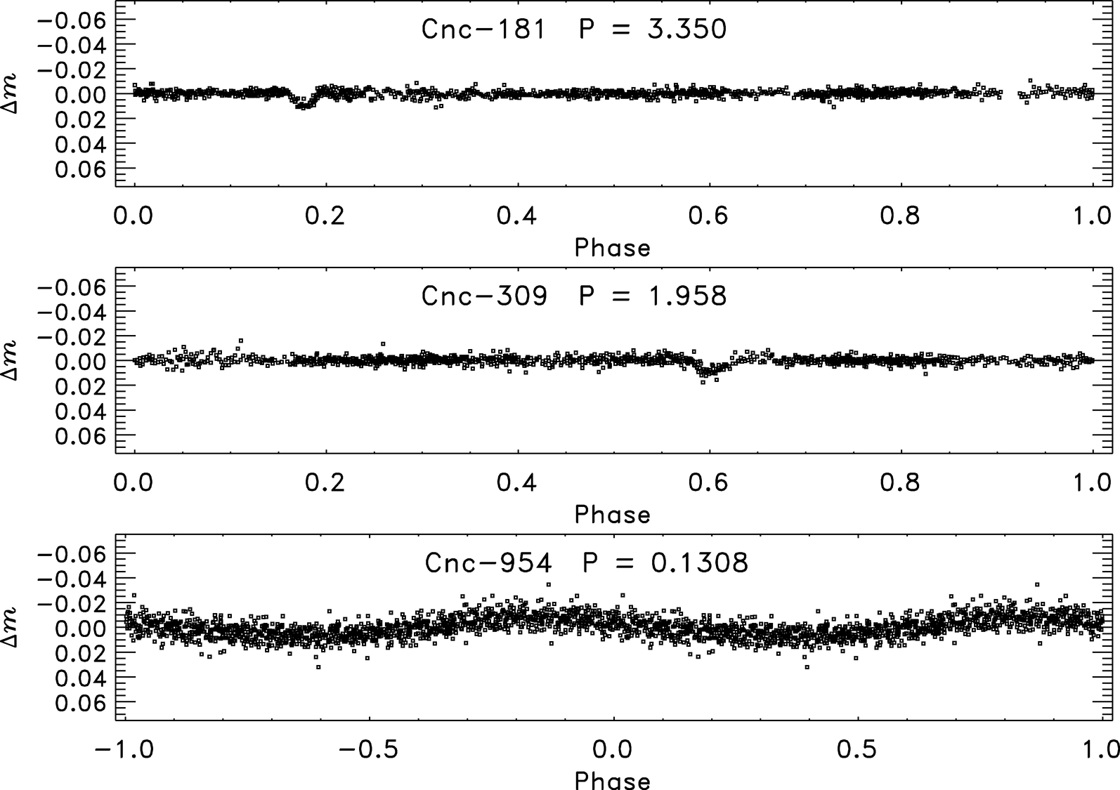
Fig. 2.— Light curves of three stars in a field centered on χ Cancri. The top two are transit candidates; the bottom one is most likely a δ Sct variable with an amplitude of 0.015 mag. Periods are in days.
Visual examination of the initial photometric results revealed several regions on the CCD where variations in the stars' light curves were highly correlated (or anticorrelated). We remove those correlated changes by regressing each star's light curve against the light curves of other stars, a technique very similar to that described in Jenkins et al. (2000). Since this method requires many more time points than stars, no more than 500 stars are decorrelated at once. This approach works very well for our data, removing correlated variations without significantly affecting the unique signals in the light curves, such as transits, eclipses, and pulsation signatures. We found, however, that the amplitude of the events decreased by about 10%–20%, which may affect the detectability of marginal transit events.
The final reduction step before the transit search is to construct average light curves by binning the decorrelated data in 0.0062 day (∼9 minute) wide bins. The typical rms for the bright stars is ∼0.005 mag before and ∼0.002 mag after the binning. For uninterrupted observations, there are on average five data points per bin.
All stars with low enough scatter (rms≤0.03 mag after binning) are searched for transit events using the box‐fitting least squares (BLS) algorithm (Kovács et al. 2002). Typically, we search for periods between 1.05 and 15 days, with 200 phase bins and a fractional transit length of 0.01–0.1. The light curves of the transit candidates are then examined visually to eliminate possible false detections, such as stars with deep eclipses or with signs of a secondary eclipse.
4. SYSTEM PERFORMANCE AND SAMPLE RESULTS
4.1. Noise Characteristics
The system specifications are summarized in Table 1 as a listing of various performance characteristics. In Figure 3, the scatter in the DIA photometry as a function of apparent magnitude is compared to theoretical noise estimates, which include contributions from the object (Poisson noise), sky, readout noise, and scintillation. For the bright, high‐S/N stars, which are of primary interest to us, the dominant noise sources are scintillation and shot (Poisson) noise from the target star itself. The contribution of scintillation was estimated using the equations in Dravins et al. (1998) for an average air mass of 1.5. For fainter stars, sky photon noise is the dominant source of scatter, which is not surprising given the large area of the PSST pixels (10'' × 10''). For brighter stars, there appears to be an additional noise source contributing ∼0.003 mag to the error balance. The most likely source of that additional scatter are small motions of the stellar images caused by guiding errors, in addition to a possible contribution from centering errors during aperture photometry and small flux errors introduced by the image interpolation. It should be noted that using an average air mass of 2.0 in the scintillation equation will bring the observed and predicted scatter into perfect agreement, so it is also possible that we have underestimated the contribution from scintillation.
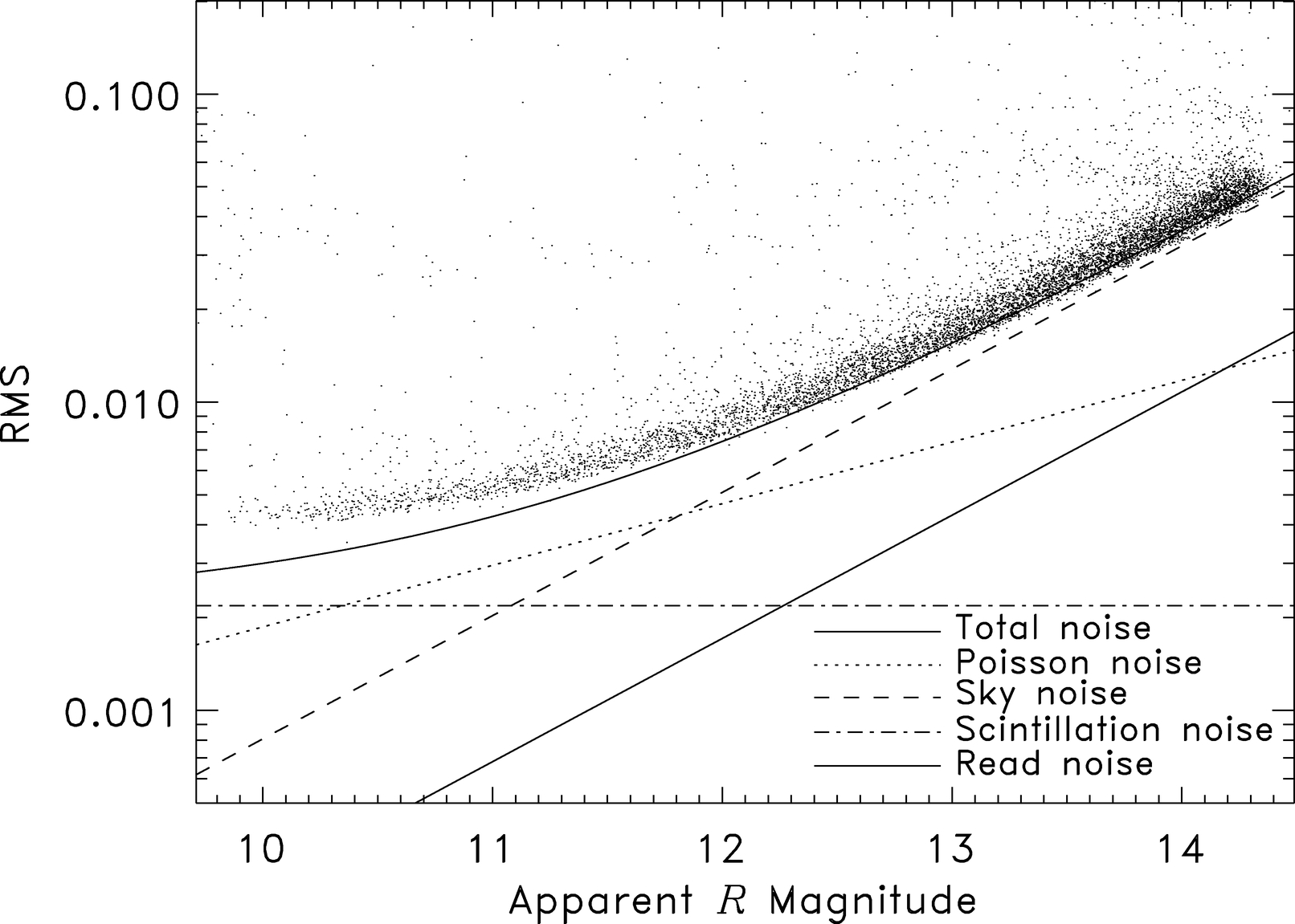
Fig. 3.— Plot of rms for the unbinned decorrelated light curves as a function of apparent R magnitude. The theoretical curves for important contributions to the total noise are also shown.
4.2. Transit Candidates
We have observed a number of fields at different Galactic latitudes and have generally found interesting candidate objects in each field. Several examples are shown in Figures 4 and 5. In Table 2 we summarize information on the fields that have been observed by PSST. Two fields at low Galactic latitudes (in Cygnus and Auriga) are not included, as the data have not yet been reduced with the DIA pipeline. The table's columns list for each field: the field and year of observation, the Galactic latitude b, the number of clear nights Nnight, the number of stars brighter than R ≈ 13, NR<13, that have been searched for transits, the number of transit candidates Ncand, the number of predicted transiting planets Npred estimated using the detection rates from Brown (2003), the number of confirmed transiting planets Ntrans, and the longest orbital period (in days) for which the probability to detect two transits exceeds 0.75. We require at least two transit‐like events in order to classify an object as a transit candidate.
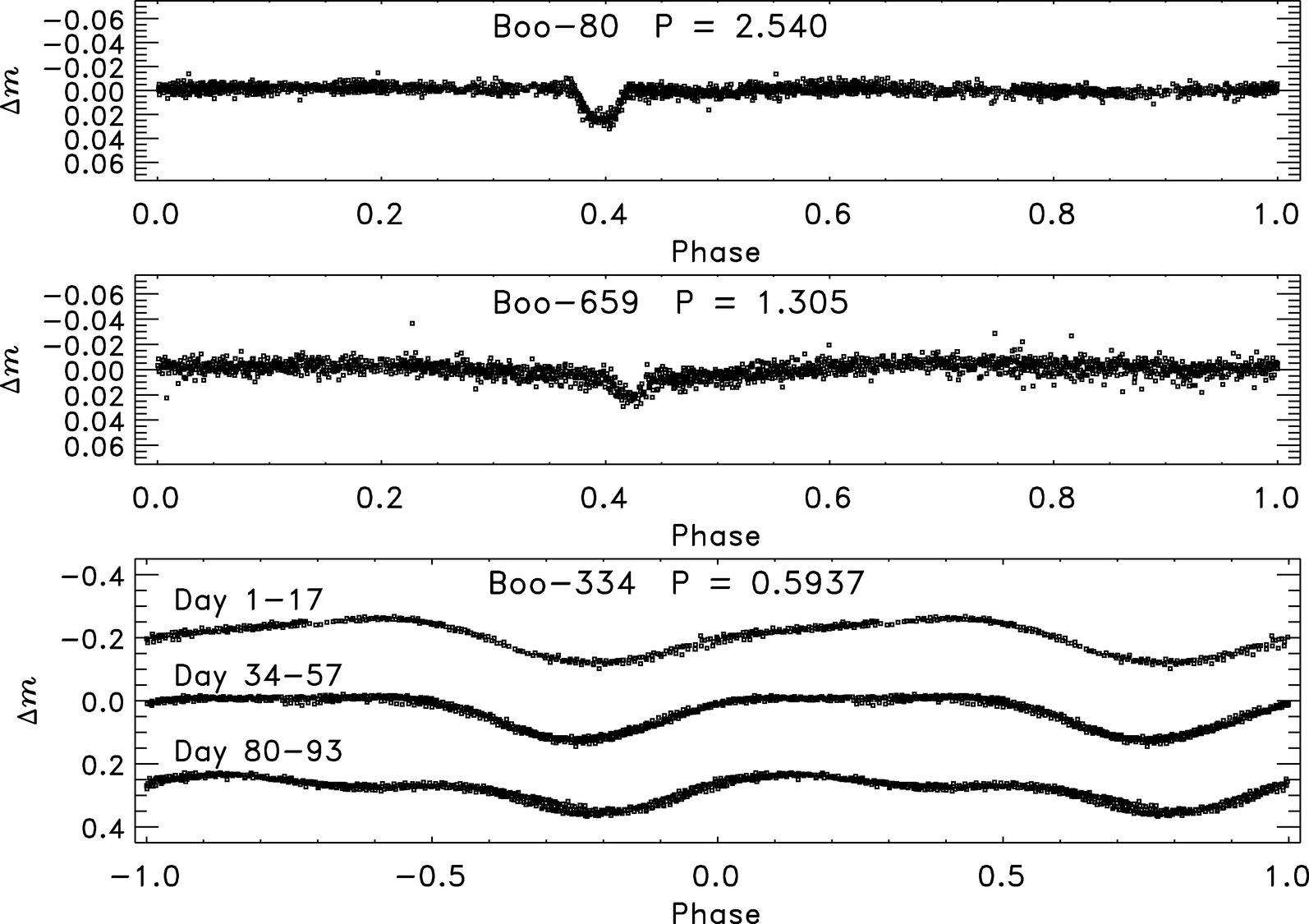
Fig. 4.— Light curves of stars in a field in Boötes observed in 2002. Top: Transit candidate later found to be an ordinary eclipsing binary. Middle: Eclipsing binary. Bottom: Star with a changing light curve shape, probably a spotted fast rotator. Periods are in days.
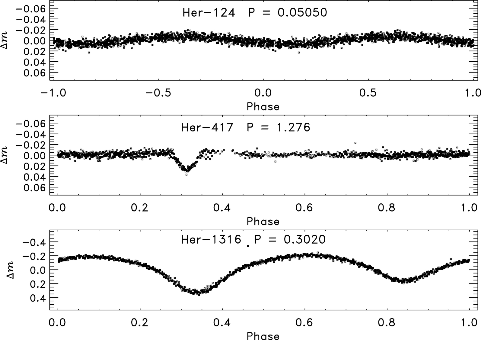
Fig. 5.— Light curves of stars in a field in Hercules observed in 2003. Top: δ Sct star with a period of 1.2 hr and amplitude of 0.012 mag. Middle: Eclipsing binary. Bottom: W UMa star. Periods are in days.
 |
While the statistics compiled in Table 2 are based only on a handful of fields, it appears that we see fewer transiting planets than predicted by the rates in Brown (2003). One reason could be that the detection rates in Brown (2003) include orbital periods of up to 30 days, whereas our observations strongly favor the discovery of short‐period transits (last column of Table 2). One solution to this problem is to monitor the same field from two or more sites distributed in longitude. That is the approach that we have adopted with our collaborators Sleuth and STARE, who are 1 hr west and 7 hr east of PSST, respectively. Together, the three telescopes form the Transatlantic Exoplanet Survey (TrES) network, which observes the same field in the sky for several weeks. As shown in Charbonneau (2004), the transit recovery rate of such a network is much higher, especially at longer periods. Indeed, the TrES network recently announced the first extrasolar planet to be discovered by a wide‐field transit search program5 (Alonso et al. 2004).
We have found that the transit candidates have a high probability of being blends involving eclipsing binary stars, low‐amplitude eclipsing binaries with an undetectable secondary minimum, grazing eclipsing binaries, or hierarchical multiple star systems (Charbonneau et al. 2004). This is consistent with the experience of Konacki et al. (2003). We have developed a follow‐up procedure to winnow out the astrophysical false positive cases. First, we use the online Digitized Sky Survey6 to check for blends inside the ∼20'' PSST stellar profile. The Two Micron All Sky Survey (2MASS) catalog (Skrutskie et al. 1997) is also often helpful for identifying whether the candidate system's primary is a giant or dwarf star (Brown 2003). Photometry with a larger telescope can be carried out if necessary to confirm whether an eclipsing binary that is blended in the PSST image profile is involved. For the more promising candidates, radial velocity observations at a sensitivity of ∼1 km s−1 are carried out by our collaborators to identify binaries with stellar secondaries. Finally, any candidate that shows no variation at this level of sensitivity is added to the target list for a high‐precision radial velocity program carried out by our collaborators.
4.3. Variable Stars
A side effect of obtaining high‐precision, high‐cadence photometry for many thousands of stars per field is the discovery of numerous variable sources. The nearly continuous coverage for a period of 7–14 weeks per field means that a catalog of short‐period variable stars for that field will be nearly complete, especially for pulsating variables and contact eclipsing binaries whose brightness varies continuously. Catalogs like these will yield a treasure trove of information on relatively bright, easy to follow up variable stars such as SX Phoenicis, β Cephei, δ Scuti, W Ursae Majoris, short‐period Cepheids and RR Lyrae variables, and other stars.
5. CONCLUSIONS
PSST is in routine, automated operation at Anderson Mesa on almost every clear night. Its shot‐noise–limited sensitivity is sufficient to detect ∼2% or less deep transits for target stars from the saturation level of R ≈ 9.8 to the limiting magnitude of R ≈ 13.0 for 0.005 mag rms. The additional longitude coverage and weather mitigation that comes from collaboration with the STARE and Sleuth projects will improve the phase coverage on each field, allowing us to collectively observe fields at a more rapid cadence than we could individually.
This work was carried out in part with support from grants NAG 5‐8271 and NAG 5‐12088 under the auspices of the NASA Origins of Solar Systems Program, and in part with support from Lowell Observatory. We thank Tim Brown for his invaluable help with the STARE software package and for many helpful discussions. We also thank David Charbonneau for providing the routine to calculate transit recovery rates, and Larry Wasserman for the essential support with the telescope control software. John Noble and Katie Morzinski provided invaluable help during operations, and Kameron Rausch helped out in the early phases of the hardware development phase. We thank the Lowell Observatory technical staff for their support throughout the program.
Footnotes
- 1
See the Stellar Astrophysics and Research on Exoplanets (STARE) Web page at http://www.hao.ucar.edu/public/research/stare/stare.html.
- 2
- 3
- 4
IRAF is distributed by the National Optical Astronomy Observatories, which is operated by the Association of Universities for Research in Astronomy, Inc., under cooperative agreement with the National Science Foundation.
- 5
The field in Lyra where the planet was discovered was observed in 2003 by both PSST and STARE. The planet's period is very close to an integral number of days (3.03), so that none of the transits in the summer of 2003 were visible on the clear nights at Lowell Observatory but were seen in the data from STARE. The circumstances of this discovery again show the advantage of longitude‐distributed transit surveys.
- 6
The Digitized Sky Survey was produced at the Space Telescope Science Institute under US government grant NAG W‐2166. The images of these surveys are based on photographic data obtained using the Oschin Schmidt Telescope on Palomar Mountain, and the UK Schmidt Telescope. The plates were processed into the present compressed digital form with the permission of these institutions.