


ABSTRACT
We report proper-motion measurements for 427 late-type M, L, and T dwarfs, 332 of which have been measured for the first time. Combining these new proper motions with previously published measurements yields a sample of 841 M7-T8 dwarfs. We combined parallax measurements or calculated spectrophotometric distances, and computed tangential velocities for the entire sample. We find that kinematics for the full and volume-limited 20 pc samples are consistent with those expected for the Galactic thin disk, with no significant differences between late-type M, L, and T dwarfs. Applying an age–velocity relation we conclude that the average kinematic age of the 20 pc sample of ultracool dwarfs is older than recent kinematic estimates and more consistent with age results calculated with population synthesis models. There is a statistically distinct population of high tangential velocity sources (Vtan > 100 km s−1) whose kinematics suggest an even older population of ultracool dwarfs belonging to either the Galactic thick disk or halo. We isolate subsets of the entire sample, including low surface gravity dwarfs, unusually blue L dwarfs, and photometric outliers in J − Ks color and investigate their kinematics. We find that the spectroscopically distinct class of unusually blue L dwarfs has kinematics clearly consistent with old age, implying that high surface gravity and/or low metallicity may be relevant to their spectral properties. The low surface gravity dwarfs are kinematically younger than the overall population, and the kinematics of the red and blue ultracool dwarfs suggest ages that are younger and older than the full sample, respectively. We also present a reduced proper-motion diagram at 2MASS (Two Micron All Sky Survey) Ks for the entire population and find that a limit of  > 18 excludes M dwarfs from the L and T dwarf population regardless of near-infrared color, potentially enabling the identification of the coldest brown dwarfs in the absence of color information.
Export citation and abstract BibTeX RIS
1. INTRODUCTION
Kinematic analyses of stars have played a fundamental role in shaping our picture of the Galaxy and its evolution. From early investigations (e.g., Schwarzschild 1908; Lindblad 1925; Oort 1927) where the large-scale structure of the Galactic disk was first explored, through more recent investigations (e.g., Gilmore & Reid 1983; Gilmore et al. 1989; Dehnen & Binney 1998; Famaey et al. 2005) where the structure of the Galaxy was refined to include a thick disk and prominent features such as streams, moving groups, and superclusters, kinematics have played a vital role in understanding the Galactic origin, evolution, and structure. Combining kinematics with spectral features, several groups have mapped out ages and metallicities for nearby F, G, K, and M stars (e.g., Nordström et al. 2004). The ages of these stars have become an important constraint on the Galactic star-formation history and their kinematics have become a vital probe for investigating membership in the young thin disk, intermediate aged thick disk, or older halo portion of the Galaxy.
One population that has yet to have its kinematics exploited is the recently discovered population of very low mass ultracool dwarfs (UCDs). These objects, which include those that do not support stable hydrogen fusion (Kumar 1962; Hayashi & Nakano 1963), occupy the late-type M through T dwarf spectral classifications (e.g., Kirkpatrick 2005, and references therein). UCDs emit the majority of their light in the infrared and thus were only discovered in large numbers with the advent of wide-field near-infrared imaging surveys such as the Two Micron All Sky Survey (2MASS; Skrutskie et al. 2006), the Deep Infrared Survey of the Southern Sky (DENIS; Epchtein et al. 1997), and the Sloan Digital Sky Survey (SDSS; York et al. 2000). Their very recent discovery has largely precluded astrometric measurements that require several-year baselines to produce useful measurements. Therefore, while UCDs appear to be comparable in number to stars (e.g., Reid et al. 1999), their role in the structure of the Galaxy is yet to be explored.
In addition, the thermal evolution of brown dwarfs (the lowest-temperature ultracool dwarfs) implies that there is no direct correlation between spectral type (SpT) and mass, leading to a mass/age degeneracy, which makes it difficult to study the mass function and formation history of these objects. While some benchmark sources (e.g., cluster members, physical companions to bright stars) have independent age determinations, and spectroscopic analyses are beginning to enable individual mass and age constraints (e.g., Burgasser et al. 2006a; Saumon et al. 2007; Mohanty et al. 2004), the majority of brown dwarfs are not sufficiently characterized to break this degeneracy. Kinematics can be used as an alternate estimator for the age of the brown dwarf population.
Moreover, kinematics can also be used to characterize subsets of UCDs. With hundreds of UCDs now known7, groupings of peculiar objects—sources whose photometric or spectroscopic properties differ consistently from the majority of the population—are becoming distinguishable. Currently defined subgroups of late-type M, L, and T dwarfs include (1) low surface gravity, very low mass objects (e.g., McGovern et al. 2004; Kirkpatrick et al. 2006; Allers et al. 2007; Cruz et al. 2007), (2) old, metal-poor ultracool subdwarfs (e.g., Burgasser et al. 2003c; Lépine et al. 2003; Gizis & Harvin 2006; Burgasser et al. 2007b), (3) unusually blue L dwarfs (UBLs; e.g., Cruz et al. 2003; Cruz et al. 2007; Knapp et al. 2004; Chiu et al. 2006), and (4) unusually red and possibly dusty L dwarfs (e.g., Looper et al. 2008; McLean et al. 2003). While observational peculiarities can overlap between these groups (e.g., both young and dusty L dwarfs can be unusually red), they appear to encompass objects with distinct physical traits (e.g., mass, age, composition, and cloud properties) so they are important for drawing a connection between observational characteristics and intrinsic physical properties. Kinematics can be used to investigate the underlying physical causes for the peculiarities of these groups.
In the past decade, a number of groups have conducted astrometric surveys of UCDs, including subsets of low-mass objects (e.g., Vrba et al. 2004; Dahn et al. 2002; Gizis et al. 2000; Tinney et al. 2003; Schmidt et al. 2007; Jameson et al. 2007; Osorio et al. 2007; West et al. 2008, 2006). We have initiated the Brown Dwarf Kinematics Project (BDKP), which aims to measure the positions and three-dimensional velocities of all known L and T dwarfs within 20 pc of the Sun and selected sources of scientific interest at larger distances (e.g., low surface gravity dwarfs, subdwarfs). In this article we add 332 new proper-motion measurements and combine all published proper-motion measurements and distance estimates into a uniform sample to examine the ultracool dwarf population as a whole. Section 2 of this paper outlines the observed sample and describes how proper-motion measurements were made. Section 3 discusses the expanded sample and how distances and Vtan measurements were calculated. Section 4 examines the full astrometric sample and subsets. Section 5 reviews the high tangential velocity objects in detail. Finally, Section 6 applies an age–velocity relation (AVR) and examines resultant ages of the full sample and red/blue outliers.
2. OBSERVATIONS AND PROPER MOTION MEASUREMENTS
2.1. Sample Selection
Our goal is to reimage all known late-type M, L, and T dwarfs to obtain accurate uniformly measured proper motions for the entire ultracool dwarf population. In our sample, we focused on the lowest-temperature L and T dwarfs that were lacking proper-motion measurements or whose proper-motion uncertainty was larger than 40 mas yr−1. We gave high priority to any dwarf that was identified as a low surface gravity object in the literature. Our sample was created from 634 L and T dwarfs listed on the Dwarf Archives Website as well as 456 M7-M9.5 dwarfs gathered from the literature (primarily from Cruz et al. 2003, 2007). The sample stayed current with the Dwarf Archives Website through April 2008. Figure 1 shows the histogram of SpT distributions for the entire sample. The late-type M dwarfs and early-type L dwarfs clearly dominate the ultracool dwarf population. Plotted in this figure is the current distribution of objects with proper-motion values and the distribution of objects for which we report new proper motions. To date we have reimaged 427 objects. As of 2008 June and including all of the measurements reported in this article, 570 of the 634 known L and T dwarfs and 277 of the 456 late-type M dwarfs in our sample have measured proper motions.

Figure 1. Spectral-type distribution of all late-type M, L, and T dwarfs. The overall histogram is the distribution of all ultracool dwarfs in our sample. The blue shaded histogram shows ultracool dwarfs with proper-motion measurements. The diagonally shaded histogram shows the distribution of ultracool dwarfs with new proper motions reported in this paper.
Download figure:
Standard image High-resolution image2.2. Data Acquisition and Reduction
Images for our program were obtained using three different instruments and telescopes in the northern and southern hemispheres. Table 1 lists the instrument properties. For the northern targets the 1.3 m telescope at the MDM observatory with the TIFKAM IR imager in the J band was used. For the southern targets the 0.9 m and 1.5 m telescopes at the Cerro Tololo Inter-American Observatory (CTIO) with the CFIM optical imager in the I band and the CPAPIR wide-field IR imager in J band (respectively) were used. The CTIO data were acquired through queue observing on 11 nights in 2007 March, September, and December, and standard user observing on nine nights in 2008 January. The MDM targets were imaged on five nights in 2007 November and seven nights in 2008 April. Objects were observed as close to the meridian as possible up to an air mass of 1.80, and with seeing no greater than 2 5 FWHM. Exposure times varied depending on the target and the instrument. For CPAPIR the exposure times ranged over 15–40 s with four coadds per image and a five-point dither pattern. At MDM the exposure times ranged over 30–120 s with up to six coadds per image and a three to five-point dither pattern. For the 0.9 m observations the exposure times ranged over 180–1800 s per image with no coadds and a three-point dither pattern. The dither offset between positions with each instrument was 10''.
Table 1. Properties of Instruments Used for Astrometric Measurements
| Telescope | Instrument | Band | FOV (arcmin) | Plate Scale (arcsec pixel−1) | Dates | Seeing (arcsec) | Sources Observed |
|---|---|---|---|---|---|---|---|
| CTIO 0.9m | CFIM | I | 4.5 | 0.40 | 2007 Sep 23–26 | 0.8–2.0 | 42 |
| MDM 1.3m | TIFKAM | J | 5.6 | 0.55 | 2007 Nov 20–24 | 1.0–2.5 | 66 |
| 2008 Apr 22–28 | 0.8–2.5 | 80 | |||||
| CTIO 1.5m | CPAPIR | J | 35.0 | 1.02 | 2005 Oct 19 | 1.0–1.5 | 4 |
| 2006 Aug 21 | 1.0–2.0 | 7 | |||||
| 2007 Mar 04 | 0.9–1.8 | 28 | |||||
| 2007 Mar 23 | 0.9–1.3 | 39 | |||||
| 2007 Dec 03–06 | 1.0–2.0 | 35 | |||||
| 2008 Jan 15–23 | 0.7–2.5 | 248 |
Download table as: ASCIITypeset image
All data were processed in a similar manner using standard IRAF and IDL routines. Dome flats were constructed in the J or I band. CPAPIR and CFIM dome flats were created from 10 images illuminated by dome lamps, and TIFKAM dome flats were created by subtracting the median of 10 images taken with all dome lights off from the median of 10 images taken with the dome lights on. A dark image constructed from 25 images taken with the shutter closed was used to map the bad pixels on the detector. Dome flats were then dark-subtracted and normalized. Sky frames were created for each instrument by median combining all of the science data that were taken on a given night. Science frames were first flat-fielded, then sky-subtracted. Individual frames were shifted and stacked to form the final combined images.
2.3. Calculating Proper Motions
The reduced science frames were astrometrically calibrated using the 2MASS Point Source catalogue. 2MASS astrometry is tied to the Tycho-2 positions and the reported astrometric accuracy varies from source to source. In general, the positions of 2MASS sources in the magnitude range 9 < Ks < 14 are repeatable to 40–50 mas in both right ascension (R.A.) and declination (decl.).
Initial astrometry was fitted by inputting a 2 × 2 transformation matrix containing astrometry parameters that were first calculated from an image in which there were two stars whose 2MASS R.A. and decl. values, and second-epoch (X, Y) pixel positions were known. The reference R.A., decl., and pixel values were first set to the pointing R.A. and decl. values and the center of the chip, respectively.
R.A. and decl. values for all the stars in the field were then imported from the 2MASS point source catalogue and converted to (X, Y) pixel positions using the initial astrometric parameters. We worked with the (X, Y) positions of the second-epoch image so that we could overplot point source positions on an image and visually check that we converged upon a best-fit solution. We detected point sources on the second-epoch image with a centroiding routine that used a detection threshold of 5σ above the background. We matched the 2MASS (X, Y) positions to the second-epoch positions by cross correlating the two lists. We refined the astrometric solution by a basic six parameter, least-squares, linear transformation where we took the positions from the 2MASS image (X1, Y1) and the positions from the second-epoch image (X0, Y0) and solved for the new (X, Y) pixel positions of the second-epoch image in the 2MASS frame. Due to the large field of view, we checked for higher-order terms in the CPAPIR images and found no significant terms. The following equations were used:


where x2o and y2o were set to the center of the field; A, B, C, and D solve for the rotation and plate scale in the two coordinates.
The sample of stars used to compute the astrometric solution for each image were selected according to the following criteria.
- 1.Only stars in the 2MASS J-magnitude range 12 < J < 15 were used, as objects in this intermediate magnitude range transformed with the smallest residuals from epoch to epoch.
- 2.The solution reference stars were required to transform with total absolute residuals of less than 0.2 pixels against 2MASS. From testing with images taken consecutively using each instrument, the best astrometric solution was always generated between 0.1 and 0.2 pixel average residuals. Therefore the stars used to calculate the solution were required to fall in or below that range.
As the solution was iterated, the residuals were examined at each step, and stars that did not fit the above criteria were removed. For CPAPIR, the process converged on a solution that had between 100 and 200 reference stars with average residuals below 0.15 pixels. TIFKAM and CFIM have smaller fields of view (∼ 6 arcmin and ∼ 5 arcmin respectively as opposed to 35 arcmin for CPAPIR) so there were far fewer stars to work with. For these imagers the process converged on a solution that had between 15 and 60 reference stars. The astrometric solution was required to converge with no less than 15 reference stars and when this criterion could not be met, the other two criteria listed above were relaxed. As a result, TIFKAM and CFIM had slightly larger residuals on the astrometric solution (average residuals less than 0.25 pixels).
Once an astrometric solution was calculated, final second-epoch positions were computed using a Gaussian fit for each 2MASS (X, Y) position on an image. For the science target, a visual check was employed to ensure that it had been detected and (X, Y) positions were manually input for the Gaussian fit. Final (X, Y) positions were then converted back into R.A. and decl. values using the best astrometric solution, and the proper motion was calculated using the positional offset and time difference between the second-epoch image and 2MASS.
The residuals of the astrometric solution were converted into proper-motion uncertainties by first multiplying by the plate scale of the instrument and then dividing by the epoch difference. The baselines ranged from 6–10 years and our astrometric uncertainties range from 5 to 50 mas yr−1. Positional uncertainties for each source were also calculated by comparing the residuals of transforming the (X, Y) positions for our target over consecutive dithered images. These uncertainties are dominated by counting statistics, with the high S/N (signal-to-noise ratio) sources having negligible positional uncertainties compared to the uncertainties in the astrometric solution. We added the positional and astrometric solution uncertainties in quadrature to determine the total proper-motion uncertainty. Figure 2 shows the distribution of proper-motion uncertainties and baselines for all new proper-motion measurements reported in this paper. The median uncertainty was 18 mas yr−1.

Figure 2. (Top): the distribution of proper-motion uncertainties for the sample of 427 measurements reported in this paper. The median value is 18 mas yr−1. (Bottom): the distribution of proper-motion baselines (time between first- and second-epoch measurements) used in this survey.
Download figure:
Standard image High-resolution imageOf the 427 proper-motion measurements we report in this paper, 332 are presented here for the first time. Twelve objects were purposely remeasured with multiple instruments as a double check on the accuracy of the astrometric solution, and 42 objects were remeasured to refine the proper-motion uncertainties. Thirty-two measurements were published in Jameson et al. (2007; hereafter J07) and 11 in Caballero (2007) while our observations were underway. The proper-motion measurements presented in this paper agree to better than 2σ in 84 of the 97 cases of objects with prior measurements. Table 2 lists those cases where the proper motions are discrepant by more than 2σ with a published value. For nine of the objects, there is a third (fourth or fifth) measurement by an independent group with which we are in good agreement. We are discrepant with six objects reported in Deacon et al. (2005) but we note that there are no position angle uncertainties reported for these objects in that catalog; therefore we cannot fully assess the accuracy of the proper-motion components. The difference in proper motion for 2MASSW J1555157−095605 is quite large (>1'' yr−1) but there are two other measurements for this object with which we are in close agreement. We have examined all of the discrepant proper-motion images carefully and see no artifacts that could have skewed our measurements. Figure 3 compares the proper-motion component measurements from this paper with those from the literature for objects with μ < 05 yr−1 and μerr < 01 yr−1. With ∼90% agreement with published results, this indicates that the 332 new measurements are robust. Table 3 contains all new measurements reported in this article, and Table 4 contains the astrometric measurements for the full sample.

Figure 3. The comparison of right ascension (top) and declination (bottom) proper motion measured in this paper and those measured in the literature. The straight line represents a perfect agreement between measurements. The red highlighted objects are the discrepant proper-motion measurements (see Table 2).
Download figure:
Standard image High-resolution imageTable 2. Discrepant Proper Motion Values
| Name | μαcos(δ) ('' yr−1) This Paper | μdecl. ('' yr−1) This Paper | μαcos(δ) ('' yr−1) Literature | μdecl. ('' yr−1) Literature | Reference |
|---|---|---|---|---|---|
| SIPS J0050−1538 | −0.229 ± 0.018 | −0.494 ± 0.019 | −0.495 ± 0.039 | −0.457 ± 0.038 | 16 |
| 2MASSJ02271036−1624479 | 0.426 ± 0.016 | −0.297 ± 0.017 | 0.509 ± 0.016 | −0.303 ± 0.010 | 16 |
| 2MASSJ09393548−2448279 | 0.592 ± 0.019 | −1.064 ± 0.021 | 0.486 ± 0.031 | −1.042 ± 0.055 | 41 |
| 2MASSWJ1155395−372735 | 0.050 ± 0.012 | −0.767 ± 0.015 | 0.113 ± 0.005 | −0.861 ± 0.039 | 16 |
| 0.013 ± 0.015 | −0.778 ± 0.013 | 9 | |||
| 0.06 ± 0.04 | −0.82 ± 0.07 | 36 | |||
| 2MASSJ13411160−3052505 | 0.030 ± 0.013 | −0.134 ± 0.015 | 0.109 ± 0.014 | −0.163 ± 0.022 | 17 |
| 2MASSJ13475911−7610054 | 0.203 ± 0.005 | 0.038 ± 0.020 | 0.257 ± 0.063 | 0.287 ± 0.063 | 22 |
| 0.193 ± 0.011 | 0.049 ± 0.019 | 35 | |||
| 2MASSWJ1448256+103159 | 0.262 ± 0.022 | −0.120 ± 0.022 | 0.70 ± 0.15 | −0.10 ± 0.16 | 36 |
| 0.249 ± 0.015 | −0.099 ± 0.016 | 10 | |||
| 2MASSWJ1507476−162738 | −0.128 ± 0.014 | −0.906 ± 0.015 | −0.043 ± 0.011 | −1.037 ± 0.255 | 16 |
| −0.1615 ± 0.0016 | −0.8885 ± 0.0006 | 15 | |||
| −0.147 ± 0.003 | −0.890 ± 0.002 | 12 | |||
| −0.09 ± 0.11 | −0.88 ± 0.06 | 36 | |||
| 2MASSJ15485834−1636018 | −0.210 ± 0.016 | −0.107 ± 0.017 | −0.189 ± 0.016 | −0.176 ± 0.015 | 17 |
| −0.098 ± 0.043 | −0.161 ± 0.042 | 22 | |||
| 2MASSWJ1555157−095605 | 0.950 ± 0.015 | −0.767 ± 0.015 | 0.929 ± 0.014 | −2.376 ± 0.017 | 10 |
| 0.961 ± 0.017 | −0.835 ± 0.014 | 16 | |||
| −0.400 ± 1.200 | −1.900 ± 1.100 | 9 | |||
| 2MASSJ19360187−5502322 | 0.169 ± 0.009 | −0.298 ± 0.016 | 0.603 ± 0.037 | −0.579 ± 0.035 | 16 |
| 0.22 ± 0.29 | −0.19 ± 0.28 | 36 | |||
| 2MASSJ22551861−5713056 | −0.216 ± 0.011 | −0.260 ± 0.020 | 0.394 ± 0.321 | −1.525 ± 0.319 | 22 |
| −0.16 ± 0.11 | −0.32 ± 0.13 | 36 | |||
| 2MASSJ23302258−0347189 | 0.223 ± 0.022 | 0.014 ± 0.022 | 0.349 ± 0.051 | −0.107 ± 0.016 | 16 |
| 0.232 ± 0.017 | 0.032 ± 0.013 | 10 |
Notes. Details on the discrepant proper-motion objects. We note only objects whose proper-motion values were discrepant by more than 2σ. Proper motion references are listed in Table 4.
Download table as: ASCIITypeset image
Table 3. New Proper Motion Measurements
| Source Name (1) | R.A. (J2000) (2) | Decl. (J2000) (3) | SpTa (optical) (4) | SpT (near-IR) (5) | μαcos(δ) ('' yr−1) (6) | μδ ('' yr−1) (7) | Baseline (yrs) (8) | Instrument (9) |
|---|---|---|---|---|---|---|---|---|
| 2MASS J00034227−2822410 | 00 03 42.27 | −28 22 41.0 | M7.5 | ... | 0.257 ± 0.016 | −0.145 ± 0.018 | 9.2 | CPAPIR |
| 2MASSI J0006205−172051 | 00 06 20.50 | −17 20 50.6 | L2.5 | ... | −0.032 ± 0.017 | 0.017 ± 0.018 | 9.5 | CPAPIR |
| 2MASS J00100009−2031122 | 00 10 00.09 | −20 31 12.2 | L0 | ... | 0.100 ± 0.022 | 0.007 ± 0.023 | 9.1 | CFIM |
| 2MASSI J0013578−223520 | 00 13 57.79 | −22 35 20.0 | L4 | ... | 0.055 ± 0.017 | −0.051 ± 0.019 | 9.4 | CPAPIR |
| 2MASS J00145575−4844171 | 00 14 55.75 | −48 44 17.1 | L2.5 | ... | 0.851 ± 0.012 | 0.289 ± 0.018 | 8.1 | CPAPIR |
| 2MASS J00165953−4056541 | 00 16 59.53 | −40 56 54.1 | L3.5 | ... | 0.201 ± 0.014 | 0.032 ± 0.018 | 8.3 | CPAPIR |
| EROS-MP J0032−4405 | 00 32 55.84 | −44 05 05.8 | L0 | ... | 0.126 ± 0.015 | −0.099 ± 0.021 | 8.4 | CPAPIR |
| 2MASS J00332386−1521309 | 00 33 23.86 | −15 21 30.9 | L4 | ... | 0.291 ± 0.016 | 0.043 ± 0.017 | 8.3 | CPAPIR |
| 2MASS J00374306−5846229 | 00 37 43.06 | −58 46 22.9 | L0 | ... | 0.049 ± 0.010 | −0.051 ± 0.020 | 8.2 | CPAPIR |
| SIPS J0050−1538 | 00 50 24.44 | −15 38 18.4 | L1 | ... | −0.229 ± 0.018 | −0.494 ± 0.019 | 9.6 | CPAPIR |
Notes. Details on the new proper-motion measurements reported in this article. See Table 4 for discovery references. aSpT refers to the spectral type of the object.
Machine-readable and Virtual Observatory (VO) versions of the table are available.
Download table as: Machine-readable (MRT)Virtual Observatory (VOT)Typeset image
Table 4. Full Astrometric Database
| Source Name (1) | Reference (2) | R.A. (J2000) (3) | Decl. (J2000) (4) | 2MASS J (mag) (5) | 2MASS Ks (mag) (6) | μαcos(δ) ('' yr−1) (7) | μδ ('' yr−1) (8) | μ Reference (9) | SpT (opt) (10) | SpT (IR) (11) | Distance (pc) (12) | Vtan (km s−1) | Noter (14) | Epoch (15) |
|---|---|---|---|---|---|---|---|---|---|---|---|---|---|---|
| SDSS J000013.54+255418.6 | 54 | 00 00 13.54 | +25 54 18.0 | 14.99 ± 0.10c | 14.73 ± 0.06c | 0.006 ± 0.019 | 0.130 ± 0.022 | 10 | ... | T4.5 | 11 ± 1 | 7 ± 1 | ... | 1998.8 |
| SDSS J000112.18+153535.5 | 54 | 00 01 12.17 | +15 35 35.5 | 15.42 ± 0.06c | 13.56 ± 0.10c | 0.150 ± 0.023 | −0.169 ± 0.015 | 10 | ... | L4 | 29 ± 6 | 31 ± 7 | ... | 2000.7 |
| 2MASS J00034227−2822410 | 20 | 00 03 42.27 | −28 22 41.0 | 13.07 ± 0.02 | 11.97 ± 0.03 | 0.257 ± 0.016 | −0.145 ± 0.018 | 19 | M7.5 | ... | 26 ± 3 | 37 ± 4 | 1998.9 | |
| GJ 1001B, LHS 102B | 37 | 00 04 34.84 | −40 44 05.8 | 13.11 ± 0.02 | 11.40 ± 0.03 | 0.644 ± 0.003 | −1.494 ± 0.002 | 23 | L5 | L4.5 | 13.0 ± 0.7j | 100.4 ± 5.2 | CB | 1999.6 |
| 2MASS J00044144−2058298 | 45 | 00 04 41.44 | −20 58 29.8 | 12.40 ± 0.02 | 11.40 ± 0.02 | 0.826 ± 0.076 | −0.009 ± 0.075 | 27 | M8 | ... | 18 ± 3 | 70 ± 14 | ... | 1999.5 |
| 2MASS J00054844−2157196 | 86 | 00 05 48.44 | −21 57 19.6 | 13.27 ± 0.03 | 12.20 ± 0.03 | 0.703 ± 0.024 | −0.119 ± 0.004 | 28 | M9 | ... | 23 ± 3 | 78 ± 11 | ... | 1999.5 |
| 2MASSI J0006205−172051 | 43 | 00 06 20.50 | −17 20 50.6 | 15.66 ± 0.07 | 14.01 ± 0.05 | −0.032 ± 0.017 | 0.017 ± 0.018 | 19 | L2.5 | ... | 43 ± 4 | 7 ± 4 | ... | 1998.5 |
| 2MASS J00070787−2458042 | 86 | 00 07 07.87 | −24 58 04.2 | 13.12 ± 0.02 | 12.06 ± 0.02 | 0.189 ± 0.022 | −0.051 ± 0.006 | 28 | M7 | ... | 30 ± 4 | 28 ± 5 | ... | 1998.9 |
| 2MASS J00100009−2031122 | 20 | 00 10 00.09 | −20 31 12.2 | 14.13 ± 0.02 | 12.88 ± 0.03 | 0.117 ± 0.020 | 0.031 ± 0.017 | 10 | L0 | ... | 30 ± 2 | 17 ± 3 | ... | 1998.6 |
| 2MASSI J0013578−223520 | 43 | 00 13 57.79 | −22 35 20.0 | 15.78 ± 0.07 | 14.04 ± 0.05 | 0.055 ± 0.017 | −0.051 ± 0.019 | 19 | L4 | ... | 35 ± 4 | 12 ± 3 | ... | 1998.6 |
Notes. Key for distance and photometry footnotes: aChiu et al. 2006 MKO photometry converted to 2MASS; bKendall et al. 2007 MKO photometry converted to 2MASS; cKnapp et al. 2004 MKO photometry converted to 2MASS; dLodieu et al. 2007 MKO photometry converted to 2MASS; eParallax from Bartlett (2007) fParallax from Costa et al. (2006); gParallax from Costa et al. (2005); hParallax from Dahn et al. (2002); iParallax from Gizis et al. (2007); jParallax from Henry et al. (2006); kParallax from Monet et al. (1992); lParallax from Perryman et al. (1997); mParallax from Thorstensen & Kirkpatrick (2003); nParallax from Tinney (1996); oParallax from Tinney et al. (2003); pParallax from van Altena et al. (1995); qParallax from Vrba et al. (2004); sBinary Distance from Bouy et al. (2003); tBinary Distance from Burgasser & McElwain (2006); uBinary Distance from Burgasser et al. (2006b); vBinary Distance from Burgasser et al. (2007b); wBinary Distance from Close et al. (2003); xBinary Distance from Forveille et al. (2005); yBinary Distance from Kirkpatrick et al. (2000); zBinary Distance from Law et al. (2006); aaBinary Distance from Liu et al. (2006); bbBinary Distance from Martín et al. (2005); ccBinary Distance from Martín et al. (2006); ddBinary Distance from McElwain & Burgasser (2006); eeBinary Distance from Reid et al. (2006); ffBinary Distance from Siegler et al. (2003); ggBinary Distance from Siegler et al. (2007); hhBinary Distance from vlmbinaries.org; iiBinary Distance from Burgasser (2007). rVLMC is a wide, very low mass companion, UBL is an Unusually Blue L dwarf, LG is a low surface gravity dwarf, YC is a dwarf linked to a young cluster, and CB is a close binary unresolved in 2MASS. References. Discovery Reference Key: (1) Artigau et al. 2006; (2) Becklin & Zuckerman 1988; (3) Berriman et al. 2003; (4) Biller et al. 2006; (5) Bouy et al. 2003; (6) Burgasser et al. 2004; (6B) Burgasser 2004a; (7) Burgasser et al. 1999; (8) Burgasser et al. 2000a; (9) Burgasser et al. 2000b; (10) Burgasser et al. 2002; (11) Burgasser et al. 2003a; (12) Burgasser et al. 2003c; (13) Burgasser et al. 2004; (14) Burgasser et al. 2003b; (15) Ruiz et al. 2001; (16) Chauvin et al. 2004; (17)Chauvin et al. 2005; (18) Chiu et al. 2006; (19) Cruz et al. 2003; (20) Cruz et al. 2007; (21) K. L. Cruz et al. (2009, in preparation); (22) Cruz & Reid 2002; (23) Dahn et al. 2002; (24) Deacon & Hambly 2007; (25) Deacon et al. 2005; (26) Delfosse et al. 1997; (27) Delfosse et al. 1999; (28)Delfosse et al. 2001; (29) Ellis et al. 2005; (30) Fan et al. 2000; (31) Folkes et al. 2007; (32) Geballe et al. 2002; (33) Gizis et al. 2000; (34) Gizis et al. 2001; (35) Gizis et al. 2003; (36) Gizis 2002; (37) EROS Collaboration et al. 1999; (38) Golimowski et al. 2004; (39) Hall 2002; (40) Hawley et al. 2002; (41) Henry et al. 2004; (42) Irwin et al. 1991; (43) Kendall et al. 2003; (44) Kendall et al. 2004; (45) Kendall et al. 2007; (46) Kirkpatrick et al. 1999; (47) Kirkpatrick et al. 2000; (48) Kirkpatrick et al. 2006; (49) J. D. Kirkpatrick et al. (2009, in preparation); (50) Kirkpatrick et al. 1997; (51) Kirkpatrick et al. 1991; (52) Kirkpatrick et al. 1993; (53) Kirkpatrick et al. 2001; (54) Knapp et al. 2004; (55) Leggett et al. 2000; (56) Lépine et al. 2002; (57) Luyten 1995; (58) Liebert & Gizis 2006; (59) Liebert et al. 2003; (60) Liu et al. 2002; (61) Lodieu et al. 2005; (62) Lodieu et al. 2002; (63) Looper et al. 2007; (64) Luhman et al. 2007; (65) Martín et al. 1999; (66) Martin et al. 1994; (67) McElwain & Burgasser 2006; (68) Ménard et al. 2002; (69) Metchev & Hillenbrand 2004; (70) Metchev & Hillenbrand 2006; (71) Mugrauer et al. 2006; (72) Nakajima et al. 1995; (73) Neuhäuser et al. 2005; (74) I. N. Reid et al. (2009, in preparation) (75) Phan-Bao et al. 2008; (76) Phan-Bao et al. 2006; (77) Phan-Bao et al. 2001; (78) Phan-Bao et al. 2003; (79) Potter et al. 2002; (80) Probst & Liebert 1983; (81) Rebolo et al. 1998; (82) Reid et al. 2000; (83) I. N. Reid et al. (2009, in preparation); (84) Reid & Cruz 2002; (85) Reid & Gilmore 1981; (86) Reylé & Robin 2004; (87) Ruiz et al. 1997; (88) Salim et al. 2003; (89) Schneider et al. 1991; (90) Schneider et al. 2002; (91) Scholz & Meusinger 2002; (92) Scholz et al. 2003; (93) Scholz et al. 2000; (94) Scholz et al. 2005; (95) Stern et al. 2007; (96) Strauss et al. 1999; (97) Teegarden et al. 2003; (98) Thorstensen & Kirkpatrick 2003; (99) Tinney et al. 2005; (100) Tinney et al. 1993; (101) Tinney et al. 1998; (102) Tinney et al. 1993; (103) Tsvetanov et al. 2000; (104) Wilson et al. 2001; (105) Wilson et al. 2003; (106) Wilson 2002; (107) Zapatero Osorio et al. 2002; (108) Looper et al. 2008; (109) Hambly et al. 2004; (110) Burgasser et al. (2007a, and references therein). References. PM reference (1) Artigau et al. 2006; (2) Bartlett 2007; (3) Burgasser 2004a; (4) Burgasser et al. 2003a; (5) Burgasser et al. 2004; (6) Burgasser et al. 2007b; (7) Burgasser et al. 2008b; (8) Burgasser et al. 2003b; (9) Caballero 2007; (10) Jameson et al. 2007; (11) Ruiz et al. 2001; (12) Costa et al. 2006; (13) Costa et al. 2005; (14) Cruz et al. 2007; (15) Dahn et al. 2002; (16) Deacon et al. 2005; (17) Deacon & Hambly 2007; (18) Ellis et al. 2005; (19) This paper; (20) Folkes et al. 2007; (21) Gizis et al. 2007; (22) Hambly et al. 2001; (23) Henry et al. 2006; (24) Kendall et al. 2003; (25) Kendall et al. 2004; (27) Kendall et al. 2007; (28) Lépine et al. 2002; (29) Luyten 1995; (30) Lodieu et al. 2005; (31) Lodieu et al. 2002; (32) Looper et al. 2007; (33) Monet et al. 1992; (34) Perryman et al. 1997; (35) Phan-Bao et al. 2008; (36) Schmidt et al. 2007; (37) Siegler et al. 2007; (38) Stern et al. 2007; (39) Teixeira et al. 2000; (40) Thorstensen & Kirkpatrick 2003; (41) Tinney et al. 2005; (42) Tinney 1996; (43) Tinney et al. 2003; (44) Vrba et al. 2004; (45) Osorio et al. 2007; (46) van Altena et al. 1995; (47) McCaughrean et al. (2004).
Machine-readable and Virtual Observatory (VO) versions of the table are available.
Download table as: Machine-readable (MRT)Virtual Observatory (VOT)Typeset image
3. DISTANCES, TANGENTIAL VELOCITIES, AND REDUCED PROPER MOTION
3.1. Expanded Sample
We extended our observational sample to include published late-type M, L, and T dwarfs with proper-motion measurements yielding a full combined sample containing 841 objects. Thirty-three percent of ultracool dwarfs in the full sample have multiple proper-motion measurements. In these cases, we chose the measurement with the smallest uncertainty for our kinematic analysis, typically objects from high-precision astrometric surveys such as Vrba et al. 2004 or Dahn et al. 2002. If there was a value discrepant by more than 2σ amongst multiple measurements (> 2) for an object then regardless of uncertainty we defaulted to the numbers that were in agreement and chose the one with the smaller uncertainty. Otherwise, if there was a discrepancy and only two measurements, we quoted the one that had the smaller uncertainty and made note of it during the analysis.
3.2. Distances and Tangential Velocities
True space velocities are a more fundamental measure of an object's kinematics than apparent angular motions, so proper motions for the complete sample were converted to tangential velocities using astrometric or spectrophotometric distances. As of 2008 January, only 79 of the 634 L and T dwarfs and 64 of the 456 late-type M dwarfs in our sample had published parallax measurements. Therefore to include the other 83% of L and T dwarfs and 87% of late-type M dwarfs in a population analysis, published absolute magnitude/SpT relations were used for calibrating distances. Dahn et al. (2002) and Vrba et al. (2004) both showed that MJ is well correlated with SpT for late-type M, L, and T dwarfs (see also West et al. 2005; Covey et al. 2007). Since the initial relations were published several investigators have revised the absolute magnitude/SpT relation after including new measurements and removing resolved binaries. In this paper, the distances for the M7-L4.5 dwarfs were calculated using the absolute 2MASS J magnitude/SpT relation in Cruz et al. (2003) and the distances for the L5–T8 dwarfs were calculated using the absolute MKO (Mauna Kea Observatory) K magnitude/SpT relation in Burgasser (2007)8. Both optical and near-IR SpTs are reported for ultracool dwarfs. For late-type M through the L dwarfs, we use the optical SpT in the distance relation when available but use near-IR SpTs when no optical SpTs are reported. We use the near-IR SpT in the distance relation for all the T dwarfs. The Cruz et al. (2003) relation was derived for the 2MASS magnitude system, while the Burgasser (2007) relation was derived using the MKO system. In reporting distances we maintain the magnitude system for which the relation was calculated, converting a 2MASS magnitude to an MKO magnitude or vice versa using the relation in Stephens & Leggett (2004) when necessary. The most recent precision photometry for many L and T dwarfs (e.g., Knapp et al 2004; Chiu et al. 2006, 2008) are reported on the MKO system; yet the majority of objects explored in this paper have measured 2MASS magnitudes. We convert MKO filter measurements to the 2MASS system when available using the conversion relations of Stephens & Leggett (2004) so that all of the ultracool dwarf photometry in Table 4 is reported on the 2MASS system.
The uncertainty in the derived distance is dominated by the uncertainty in the SpT (the photometric uncertainties are typically between 0.02–0.1 mag whereas the SpT uncertainties are typically 0.5–1.0). This leads to a systematic over or underestimation of distance by up to 30%. Therefore the kinematic results presented in this paper are largely sensitive to the reliability of the spectrophotometric distances used to calculate Vtan. Furthermore, unresolved multiplicity leads to an underestimation of distance. Recent work has shown that roughly 20% of ultracool dwarfs are likely to be binary (Allen 2007; Reid et al. 2008), and this fraction may be even higher across the L dwarf/T dwarf transition (Burgasser et al. 2006b). Seven percent (56) of the dwarfs analyzed in this paper are known to be close binaries and of these, most appear to be near equal-mass/equal-brightness (e.g., Bouy et al. 2003; Burgasser et al. 2006b). For these objects we use the distances quoted in the binary discovery papers where the contribution of flux from the secondary was included in the distance estimate. Any remaining tight binaries probably constitute no more than 10%–20% of the sample and the contamination due to their inclusion in the kinematic analysis is relatively small.
3.3. Reduced Proper-Motion Diagram
A reduced proper-motion diagram is a useful tool for distinguishing between kinematically distinct stellar and substellar populations. This parameter was used extensively in early, high proper-motion catalogs to explore Galactic structure (Luyten 1973). Proper motion is used as a proxy for distance measurements following the expectation that objects with large proper motions will be nearest to the Sun. The definition is analogous to that of absolute magnitude:

or

where m and M are the apparent and absolute magnitudes (respectively), Vtan is measured in km s−1, and μ is measured in arcsec yr−1.
We can use reduced proper motion to search for the lowest-temperature objects. In Figure 4, we show the reduced proper motion at Ks for our astrometric sample. We find that below an  of 18 there are only L and T dwarfs regardless of near-IR color. Since the discovery of the first brown dwarfs, near-IR color selection has been the primary technique for identifying strong candidates. But because M dwarfs dominate photometric surveys (they are bright, nearby, and found in large numbers), near-IR color cut-offs were administered to maximize the L and T dwarfs found in searches. These cut-offs have caused a gap in the near-IR color distribution of the brown dwarf population, particularly around J − Ks equal to 1 where early-type T dwarfs and metal-weak L dwarfs are eliminated along with M dwarfs. A reduced proper-motion diagram with the cut-off limit cited above allows a search that eliminates the abundant M dwarfs and probes the entire range of J − Ks colors for the ultracool dwarf population.
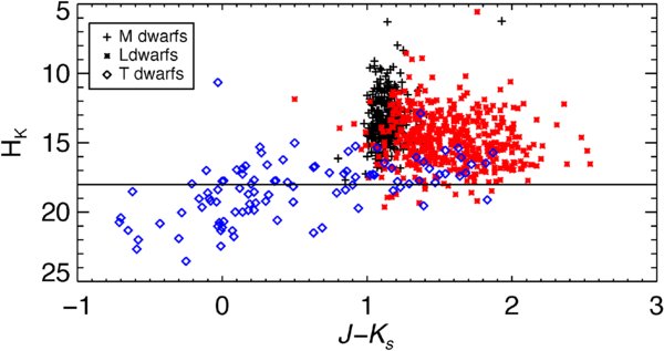
Figure 4. The reduced proper-motion diagram using the 2MASS J and Ks magnitudes. Late-type M dwarfs are marked with a black plus sign, L dwarfs are marked as a red five point star, and T dwarfs are marked as blue diamonds. The line at HK of 18 marks where M dwarfs are segregated from the L and T dwarfs regardless of near-IR color. This cut-off will also include subdwarfs and cool white dwarfs but these objects will be rare.
Download figure:
Standard image High-resolution imageNote that, while our cut-off limits are good guidelines for segregating the coolest temperature dwarfs within the ultracool dwarf population, there is likely to be contamination in selected regions of the sky from relatively rare ultracool subdwarfs and cool white dwarfs, which are nonetheless of scientific interest.
4. ANALYSIS
4.1. Kinematic Characteristics of the Ultracool Dwarf Population
The ultracool dwarfs analyzed in this paper have a range of proper-motion values from 001 yr−1–47 yr−1 and a range of proper-motion uncertainties from 00002 yr−1–03 yr−1. While one of our goals is to refine proper-motion measurements of ultracool dwarfs to have uncertainties less than 40 mas yr−1, there are still 86, or 10% that have larger errors. Since the uncertainty in Vtan is generally dominated by the uncertainty in distance (see Section 3.2) we make no restrictions on the accuracy of the proper-motion measurements used in the kinematic analysis. The median 1σ detection limit for proper-motion measurements in this paper was 18 mas yr−1 (see Figure 2). We use this value as a proxy for the L and T dwarfs (where we are looking at most of the known field objects as opposed to the late-type M dwarfs where we are looking at only a subset) to determine the percentage of objects with appreciable motion. We find that 32 move slower than our 2σ detection limit and 10 of those are at or below our 1σ limit. This indicates that according to our astrometric standard, less than 6% of L and T dwarfs have no appreciable motion. Conversely, 32 objects (or 6% of the population) move faster than 10 yr−1 making them some of the fastest known proper-motion objects. As late-type dwarfs are intrinsically quite faint and have only been detected at nearby distances (generally ⩽ 60 pc), the high proper-motion values measured are not surprising. Using the median proper-motion values listed in Table 5 as a proxy, we can also conclude that at least half or more of the brown dwarf population would be easily detectable on a near-IR equivalent of Luyten's 2-tenth catalog (Luyten 1979) where the limiting proper motion was ∼ 015 yr−1.
Table 5. Median Photometric and Kinematic Properties of Ultracool Dwarfs
| SpT (1) | Nμ (2) | μmedian ('' yr−1) (3) | σμ ('' yr−1) (4) | Median Distance (pc) (5) | σdist (pc) (6) |  (7) (7) |
(J − Ks)avg (8) | 2* (9) (9) |
NRed (10) | NBlue (11) |
|---|---|---|---|---|---|---|---|---|---|---|
| M7 | 88 | 0.261 | 0.553 | 25 | 10 | 160 | 1.08 | 0.19 | 0 | 1 |
| M8 | 114 | 0.210 | 0.403 | 23 | 8 | 147 | 1.14 | 0.18 | 1 | 1 |
| M9 | 71 | 0.204 | 0.357 | 22 | 10 | 107 | 1.20 | 0.22 | 1 | 0 |
| L0 | 93 | 0.111 | 0.211 | 32 | 19 | 92 | 1.31 | 0.37 | 4 | 1 |
| L1 | 83 | 0.208 | 0.301 | 31 | 21 | 82 | 1.39 | 0.37 | 4 | 1 |
| L2 | 58 | 0.185 | 0.209 | 32 | 17 | 63 | 1.52 | 0.40 | 5 | 1 |
| L3 | 64 | 0.189 | 0.398 | 33 | 17 | 67 | 1.65 | 0.39 | 1 | 1 |
| L4 | 50 | 0.183 | 0.284 | 27 | 12 | 44 | 1.73 | 0.40 | 2 | 2 |
| L5 | 43 | 0.323 | 0.281 | 24 | 12 | 43 | 1.74 | 0.40 | 0 | 1 |
| L6 | 36 | 0.215 | 0.339 | 26 | 12 | 31 | 1.75 | 0.40 | 4 | 2 |
| L7 | 21 | 0.247 | 0.186 | 23 | 9 | 15 | 1.81 | 0.40 | 0 | 2 |
| L8 | 16 | 0.280 | 0.368 | 19 | 8 | 16 | 1.77 | 0.33 | 2 | 0 |
| L9 | 3 | 0.424 | 0.200 | 20 | 6 | 7 | 1.69 | 0.19 | 0 | 0 |
| T0 | 9 | 0.333 | 0.165 | 18 | 4 | 8 | 1.63 | 0.40 | 0 | 0 |
| T1 | 11 | 0.289 | 1.336 | 23 | 9 | 10 | 1.31 | 0.40 | 1 | 1 |
| T2 | 13 | 0.350 | 0.285 | 15 | 7 | 15 | 1.02 | 0.40 | 1 | 0 |
| T3 | 7 | 0.183 | 0.135 | 26 | 6 | 5 | 0.63 | 0.40 | 1 | 0 |
| T4 | 13 | 0.323 | 0.219 | 23 | 9 | 6 | 0.26 | 0.40 | 0 | 0 |
| T5 | 20 | 0.340 | 0.351 | 15 | 3 | 12 | 0.07 | 0.39 | 0 | 0 |
| T6 | 15 | 0.594 | 1.217 | 11 | 18 | 5 | −0.30 | 0.40 | 2 | 1 |
| T7-T8 | 13 | 1.218 | 0.764 | 9 | 3 | 6 | −0.08 | 0.40 | 0 | 1 |
| M7-M9 | 273 | 0.222 | 0.445 | 23 | 9 | 414 | 1.12 | 0.22 | 2 | 2 |
| L0-L9 | 467 | 0.189 | 0.292 | 29 | 17 | 460 | 1.53 | 0.40 | 22 | 11 |
| T0-T9 | 101 | 0.373 | 0.801 | 15 | 10 | 67 | 0.74 | 0.40 | 5 | 3 |
Notes. To calculate the (J − Ks)avg for each SpT, we chose only objects that were not identified as binaries, young cluster members, subdwarfs and/or had σJ and  less than 0.20.
Download table as: ASCIITypeset image
Table 5 lists the average proper-motion values and photometric data for the entire population binned by SpT. There is a trend within these data for larger proper-motion values with increasing SpT. This is clearest within the L0–L9 population where the sample is the largest. We further bin this group into thirds to compare a statistically significant sample. We examine the L0–L2, L3–L5, and L6–L9 populations and find the median proper-motion values to increase as 0174 yr−1, 0223 yr−1, and 0289 yr−1, respectively. This trend most likely reflects the fact that earlier-type sources are detected to further distances. Indeed when we examine the median distance values for these same groupings we find values of 31, 27, and 20 pc, respectively.
4.2. Kinematics of Full and 20 pc Samples
We have conducted our kinematic analysis on two samples: the full astrometric sample and the 20 pc sample. Figure 5 shows the distance distribution for all ultracool dwarfs regardless of proper-motion measurements to demonstrate the pertinence of the 20 pc sample. In this figure, both the late-type M and L dwarfs diverge from an N ∝ d3 density distribution around 20 pc. The T dwarfs diverge closer to 15 pc. Within the literature (e.g., Cruz et al. 2003) complete samples up to 20 pc have been reported through mid-type L dwarfs so we use this distance in order to establish a volume-limited kinematic sample. We also examine the two samples with and without objects with Vtan >100 km s−1 in order to remove extreme outliers that may comprise a different population.

Figure 5. Cumulative distance distribution of all late-type M, L, and T dwarfs in our database. The triangles refer to the M7–M9 dwarfs, the "X" symbols refer to all L0–L9 dwarfs, and the plus symbols refer to all T0–T8 dwarfs. The solid line corresponds to a constant density distribution (N ∝ d3). The L and M dwarfs deviate from this distribution around 20 pc but the T dwarfs fall off closer to 15 pc.
Download figure:
Standard image High-resolution imageTables 6 and 7 contain the mean kinematic properties for the 20 pc sample and the full astrometric sample, respectively. Figure 6 shows Vtan versus SpT for both samples. As demonstrated in Figure 6, we find no difference between the two samples, with median Vtan values of 26 km s−1 and 29 km s−1 and σtan values of 23 km s−1 and 25 km s−1 for M7-T9 within the full sample and the 20 pc sample, respectively. Within spectral class bins, namely the M7–M9, L0–L9, or T0–T9 groupings, we find no significant kinematic differences. This indicates that we are sampling a single kinematic population regardless of the distance and SpT.

Figure 6. The distribution of Vtan values binned by SpT. The top panel is the full astrometric sample and the bottom panel is the 20 pc sample. The asterisks refer to the median Vtan values and the vertical bars refer to the standard deviation or dispersion of velocities.
Download figure:
Standard image High-resolution image
Figure 7. The overall histogram is the tangential velocity distribution for the entire sample and the diagonally shaded histogram is the 20 pc sample. Both Vtan distributions peak in the 10–30 km s−1 bins.
Download figure:
Standard image High-resolution imageTable 6. 20 pc Sample
| SpT (1) | N (2) | N High Vtan (3) | Median Vtan (km s−1) (4) | Median Vtan with High Vtan (5) | σtan (km s−1) (6) | σtan with High Vtan (km s−1) (7) | Age (Gyr) (8) | Age with High Vtan (Gyr) (9) |
|---|---|---|---|---|---|---|---|---|
| M7 | 29 | 0 | 25 | 25 | 20 | 20 | ... | ... |
| M8 | 37 | 1 | 33 | 33 | 20 | 25 | ... | ... |
| M9 | 27 | 1 | 26 | 26 | 22 | 26 | ... | ... |
| L0 | 9 | 0 | 19 | 19 | 21 | 21 | ... | ... |
| L1 | 19 | 0 | 30 | 30 | 29 | 29 | ... | ... |
| L2 | 10 | 0 | 27 | 27 | 16 | 16 | ... | ... |
| L3 | 12 | 3 | 32 | 38 | 20 | 46 | ... | ... |
| L4 | 15 | 1 | 27 | 27 | 20 | 28 | ... | ... |
| L5 | 16 | 0 | 27 | 27 | 21 | 21 | ... | ... |
| L6 | 10 | 0 | 28 | 28 | 24 | 24 | ... | ... |
| L7 | 9 | 0 | 30 | 30 | 9 | 9 | ... | ... |
| L8 | 12 | 0 | 25 | 25 | 20 | 20 | ... | ... |
| L9 | 2 | 0 | 41 | 41 | 0 | 0 | ... | ... |
| T0 | 6 | 0 | 32 | 32 | 15 | 15 | ... | ... |
| T1 | 3 | 0 | 66 | 66 | 28 | 28 | ... | ... |
| T2 | 8 | 0 | 26 | 26 | 5 | 5 | ... | ... |
| T3 | 1 | 0 | 39 | 39 | 0 | 0 | ... | ... |
| T4 | 5 | 0 | 21 | 21 | 16 | 16 | ... | ... |
| T5 | 20 | 0 | 21 | 21 | 23 | 23 | ... | ... |
| T6 | 14 | 0 | 44 | 44 | 22 | 22 | ... | ... |
| T7 | 10 | 1 | 45 | 54 | 15 | 34 | ... | ... |
| T8 | 3 | 0 | 57 | 57 | 8 | 8 | ... | ... |
| M7-M9 | 93 | 2 | 29 | 29 | 21 | 24 | 3.0+1.0−0.8 | 5.0+1.7−1.4 |
| L0-L9 | 114 | 5 | 27 | 27 | 21 | 26 | 3.2+1.1−0.9 | 6.6+2.2−1.8 |
| T0-T9 | 70 | 1 | 30 | 31 | 20 | 24 | 2.8+1.0−0.8 | 4.6+1.6−1.3 |
Notes. The age range is calculated from the Wielen (1977) AVR for the disk which uses a value of (1/3) for α.
Download table as: ASCIITypeset image
Table 7. Full Astrometric Sample
| SpT (1) | N (2) | N High Vtan (3) | Median Vtan (km s−1) (4) | Median Vtan with High Vtan (km s−1) (5) | σtan (km s−1) (6) | σtan with High Vtan (km s−1) (7) | Age (Gyr) (8) | Age with High Vtan (Gyr) (9) |
|---|---|---|---|---|---|---|---|---|
| M7 | 88 | 0 | 27 | 27 | 19 | 19 | ... | ... |
| M8 | 114 | 1 | 27 | 27 | 21 | 23 | ... | ... |
| M9 | 71 | 1 | 23 | 23 | 19 | 21 | ... | ... |
| L0 | 93 | 1 | 19 | 19 | 16 | 21 | ... | ... |
| L1 | 83 | 2 | 32 | 33 | 23 | 27 | ... | ... |
| L2 | 58 | 0 | 26 | 26 | 18 | 18 | ... | ... |
| L3 | 64 | 3 | 30 | 32 | 18 | 27 | ... | ... |
| L4 | 50 | 1 | 25 | 27 | 20 | 23 | ... | ... |
| L5 | 43 | 0 | 25 | 25 | 20 | 20 | ... | ... |
| L6 | 36 | 1 | 26 | 27 | 18 | 24 | ... | ... |
| L7 | 21 | 1 | 28 | 28 | 13 | 22 | ... | ... |
| L8 | 16 | 0 | 25 | 25 | 19 | 19 | ... | ... |
| L9 | 3 | 0 | 38 | 38 | 17 | 17 | ... | ... |
| T0 | 9 | 0 | 26 | 26 | 13 | 13 | ... | ... |
| T1 | 11 | 0 | 31 | 31 | 25 | 25 | ... | ... |
| T2 | 13 | 0 | 26 | 26 | 11 | 11 | ... | ... |
| T3 | 7 | 0 | 25 | 25 | 10 | 10 | ... | ... |
| T4 | 13 | 0 | 32 | 32 | 22 | 22 | ... | ... |
| T5 | 20 | 0 | 21 | 21 | 23 | 23 | ... | ... |
| T6 | 15 | 0 | 36 | 36 | 23 | 23 | ... | ... |
| T7 | 10 | 1 | 45 | 54 | 15 | 34 | ... | ... |
| T8 | 3 | 0 | 57 | 57 | 8 | 8 | ... | ... |
| M7-M9 | 273 | 3 | 26 | 26 | 19 | 21 | 2.5+0.9−0.7 | 3.2+1.1−0.9 |
| L0-L9 | 467 | 10 | 26 | 26 | 19 | 23 | 2.5+0.9−0.7 | 4.5+1.6−1.3 |
| T0-T9 | 101 | 1 | 29 | 29 | 20 | 23 | 2.7+1.0−0.8 | 4.0+1.4−1.1 |
Notes. The age range is calculated from the Wielen (1977) AVR for the disk which uses a value of (1/3) for α.
Download table as: ASCIITypeset image
Figure 7 shows the distribution of tangential velocities. There are 14 objects with Vtan >100 km s−1 that fall at the far end of the distribution. Exclusion of these high-velocity dwarfs naturally reduces the median Vtan and σtan values. The most significant difference in their exclusion occurs within the L0–L9 group as 10 of the 14 objects belong to that spectral class. We explore the importance of this subset of the ultracool dwarf population in Section 5.
In order to put our kinematic measurements in the context of the Galaxy, we compare with Galactic U, V, and W dispersions. Proper motion, distance, and radial velocity are all required to compute these space velocities. Therefore, a direct Galactic U, V, and W comparison with the ultracool dwarf population is not possible because radial velocity measurements for ultracool dwarfs are sparse, with only 48 of the L and T dwarfs to date having been reported in the literature (e.g., Mohanty & Basri 2003; Osorio et al. 2007; Bailer-Jones 2004). This is a similar problem to that for precise brown dwarf parallax measurements, but there is no relationship for estimating radial velocities as there is for estimating distances. However, we can divide our sample into three groups along Galactiocentric coordinate axes (toward poles, in the direction of Galactic rotation and radially to/from the Galactic center) in order to minimize the importance of radial velocity in two out of the three space velocity components. We create cones of 0 (all inclusive), 30, and 60 degrees around the galactic X, Y, and Z axes. Inside of each cone we set either the U, V, or W velocity to zero if the cone surrounds the galactic X, Y, or Z axes, respectively. In this way, we can set the radial velocity of each source to zero with minimum impact on the component velocities of the entire sample and gather U, V, and W information for the known ultracool dwarf population. We emphasize that this analysis is crude as the distribution of ultracool dwarfs is not isotropic (the Galactic plane has largely not been explored), and while the cones help to minimize the importance of radial velocity unless an object is directly on the X, Y, or Z axes, the radial velocity component will contribute to the overall velocities. Therefore, the spread of U, V, and W velocities will be biased toward a tighter dispersion than the true values. In order to calculate total velocities (Vtot) for objects, which requires U, V, and W velocities we choose a cone of 30 degrees which provides a statistically significant sample. We create the cone around the X, Y, or Z axes and assume that within that cone either the (V, W), (U, Z), or (U, V) components, respectively, are correct. To obtain the third component we assume it to be the average of the two calculated ones. In this way we can gather Vtot information which will be used for age calculation purposes in Section 6.
Figure 8 shows our resultant U, V, and W distributions where we measure (σU, σV, σW) = (28, 22, 17) km s−1. We compare these dispersions with the kinematic signatures of the three Galactic populations, namely the thin disk, the thick disk, and the halo. The overwhelming majority of stars in the solar neighborhood are members of the Galactic disk and these are primarily young thin-disk objects as opposed to older thick-disk objects. The halo population of the Galaxy encompasses the oldest population of stars in the Galaxy but these objects are relatively sparse in the vicinity of the Sun. Membership in any Galactic population has implications on the age and metallicity of the object and kinematics play a large part in defining the various populations. Soubiran et al. (2003) find (σU, σV, σW) = (39 ± 2, 20 ± 2, 20 ± 1) km s−1 for the thin disk and (σU, σV, σW) = (63 ± 6, 39 ± 4, 39 ± 4) km s−1 for the thick disk, and Chiba & Beers (2000) find (σU, σV, σW) = (141 ± 11, 106 ± 9, 94 ± 8) km s−1 for the halo portion of the Galaxy. Our U, V, and W dispersions are consistent (albeit narrower in U) with that of the Galactic thin disk.

Figure 8. A histogram of U, V, and W velocities. Plotted for each velocity is (1) each object in the astrometric sample (large histogram) (2) a 30 deg restriction on objects and (3) a 60 deg restriction (smallest histogram). The 30 and 60 deg restrictions are placed on the X, Y, or Z axes and correspond to removing the U, V, or W velocity respectively for objects in cones of noted radius around the respective axis.
Download figure:
Standard image High-resolution imageOsorio et al. (2007; hereafter Os07) examined 21 L and T dwarfs and found (σU, σV, σW) = (30.2, 16.5, 15.8) km s−1. Their velocity dispersions are tighter than what is expected for the Galactic thin-disk population. Our calculated dispersions are tighter at U than the Os07 result (which is expected due to the stated bias) but broader in V and W. In Section 6, we discuss the implications on age of the differences calculated from our astrometric sample.
4.3. Red and Blue Photometric Outliers
As discussed in Kirkpatrick (2005) the large number of late-type M, L, and T dwarfs discovered to date has revealed a broad diversity of colors and spectral characteristics, including specific subgroups of peculiar sources that are likely related by their common physical properties. As a very basic metric, near-IR colors provide one means of distinguishing between "normal" and "unusual" objects. To investigate our sample for kinematically distinct photometric outliers, we first defined the average color ((J − Ks)avg) as well as standard deviation ( ) as a function of SpT using all known ultracool dwarfs (i.e., both with and without proper-motion measurements). Defining the (J − Ks)avg for spectral bins has been done in previous ultracool dwarf studies such as Kirkpatrick et al. (2000), Vrba et al. (2004), and West et al. (2008), but we have included all ultracool dwarfs in the dwarf archives compilation and the updated photometry reported in Chiu et al. (2006, 2008) and Knapp et al. (2004), which we have converted from the MKO system to the 2MASS system. Objects were eliminated from the photometric sample if they fit any of the following criteria.
- 1.uncertainty in J or Ks greater than 0.2 magnitude;
- 2.known subdwarf;
- 3.
- 4.
We then designated objects as photometric outliers if they satisfied the following criterion:

In other words, if an object's J − Ks color was more than twice the standard deviation of the color range for that spectral bin than we flagged it as a red or blue photometric outlier. If twice the standard deviation was larger than 0.4 mag then it was automatically reset to 0.4. We chose 0.4 as the maximum upper limit for  as this is the
  for the entire ultracool dwarf population.
There are relatively few objects in each spectral bin beyond L9. For SpT < L9 there is a mean of 45 objects used per bin whereas for SpT > L9 there is a mean of only seven objects. So photometric outliers are difficult to define for the lower temperature classes and may contaminate the analysis. We grouped T7–T8 dwarfs to improve the statistics used to calculate average values. The kinematic results for this subset of the ultracool dwarf population are reported with and without the T dwarfs in Table 8. Figure 9 shows the resulting J − Ks color distribution and highlights the photometric outliers. Tables 9 and 10 list the details of the red and blue photometric outliers, respectively. Table 5 lists the resultant mean photometric values for each SpT.
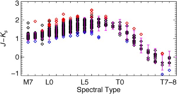
Figure 9. J − Ks colors of late-type dwarfs. We compute the average values for each SpT (binned by 1 subtype) from the 2MASS photometry of a select sample of dwarfs and then flag objects as photometric outliers when they are either twice the standard deviation of J − Ks or 0.4 mag redder or bluer than the average value. The red symbols above the plotted range of J − Ks colors are the red outliers and blue symbols below the plotted range of J − Ks colors are the blue outliers.
Download figure:
Standard image High-resolution imageTable 8. Average Kinematics and Ages for the Subgroups
| SpT (2) | N (2) | Median Vtan (km s−1) (3) | σtan (km s−1) (4) | Age Range (Gyr) (5) |
|---|---|---|---|---|
| M7-T9/BLUE | 16 | 53 | 47 | 37.9+12.6−10.3 |
| M7-T9/RED | 29 | 26 | 16 | 1.2+0.5−0.4 |
| M7-L9/BLUE | 13 | 56 | 50 | 46.0+15.2−12.4 |
| M7-L9/RED | 24 | 26 | 15 | 1.0+0.4−0.3 |
| UBLs | 10 | 99 | 47 | 37.9+12.6−10.3 |
| Low Gravity | 26 | 18 | 15 | 1.0+0.4−0.3 |
Notes. The age range is calculated from the Wielen (1977) AVR for the disk which uses a value of (1/3) for α.
Download table as: ASCIITypeset image
Table 9. Details on Red Photometric Outliers
| Source Name (1) | 2MASS J (mag) (2) | 2MASS Ks (mag) (3) | μαcos(δ) ('' yr−1) (4) | μδ (''yr−1) (5) | μ Reference (6) | SpT (opt) (7) | SpT (IR) (8) | Vtan (km s−1) (10) | Noter (11) |
|---|---|---|---|---|---|---|---|---|---|
| 2MASS J00374306−5846229 | 15.37 ± 0.05 | 13.59 ± 0.05 | 0.049 ± 0.010 | −0.051 ± 0.020 | 19 | L0 | ... | 18 ± 5 | LG |
| SDSSp J010752.33+004156.1 | 15.82 ± 0.06 | 13.71 ± 0.04 | 0.628 ± 0.007 | 0.091 ± 0.004 | 44 | L8 | L5.5 | 46.9 ± 3.3 | ... |
| 2MASS J01244599−5745379 | 16.31 ± 0.11 | 14.32 ± 0.09 | −0.003 ± 0.010 | 0.018 ± 0.019 | 19 | L0 | ... | 7 ± 7 | LG |
| 2MASS J01415823−4633574 | 14.83 ± 0.04 | 13.10 ± 0.03 | 0.104 ± 0.017 | −0.026 ± 0.024 | 19 | L0 | L0 | 21 ± 4 | LG |
| 2MASS J01490895+2956131 | 13.45 ± 0.02 | 11.98 ± 0.02 | 0.1757 ± 0.0008 | −0.4021 ± 0.0007 | 15 | M9.5 | ... | 46.8 ± 0.7 | ... |
| 2MASSI J0243137−245329 | 15.42 ± 0.06c | 15.22 ± 0.06c | −0.288 ± 0.004 | −0.208 ± 0.003 | 44 | ... | T6 | 18.0 ± 0.7 | ... |
| 2MASS J03231002−4631237 | 15.39 ± 0.07 | 13.70 ± 0.05 | 0.060 ± 0.013 | −0.010 ± 0.019 | 19 | L0 | ... | 16 ± 4 | LG |
| 2MASS J03264225−2102057 | 16.13 ± 0.09 | 13.92 ± 0.07 | 0.108 ± 0.014 | −0.146 ± 0.015 | 19 | L4 | ... | 35 ± 5 | ... |
| 2MASS J03421621−6817321 | 16.85 ± 0.14 | 14.54 ± 0.09 | 0.064 ± 0.007 | 0.021 ± 0.018 | 19 | L2 | ... | 26 ± 5 | ... |
| 2MASS J03552337+1133437 | 14.05 ± 0.02 | 11.53 ± 0.02 | 0.192 ± 0.017 | −0.613 ± 0.017 | 19 | L5 | ... | 25 ± 5 | LG |
| 2MASS J04351455−1414468 | 11.88 ± 0.03 | 9.95 ± 0.02 | 0.009 ± 0.014 | 0.016 ± 0.014 | 19 | M8 | ... | 1 ± 1 | LG |
| 2MASS J05012406−0010452 | 14.98 ± 0.04 | 12.96 ± 0.04 | 0.158 ± 0.014 | −0.139 ± 0.014 | 19 | L4 | ... | 24 ± 5 | LG |
| 2MASSI J0512063−294954 | 15.46 ± 0.06 | 13.29 ± 0.04 | −0.028 ± 0.016 | 0.099 ± 0.018 | 19 | L4.5 | ... | 13 ± 3 | ... |
| 2MASS J05361998−1920396 | 15.77 ± 0.08 | 13.85 ± 0.06 | 0.017 ± 0.017 | −0.024 ± 0.018 | 19 | L1 | ... | 8 ± 5 | ... |
| AB Pic b | 16.18 ± 0.10 | 14.14 ± 0.08 | 0.0141 ± 0.0008 | 0.0452 ± 0.0010 | 34 | ... | L1 | 10.2 ± 0.4 | VLMC |
| SDSS J080959.01+443422.2 | 16.51 ± 0.06c | 14.34 ± 0.06c | −0.198 ± 0.014 | −0.214 ± 0.019 | 19 | ... | L6 | 35 ± 7 | ... |
| SDSS J085834.42+325627.7 | 16.52 ± 0.06a | 14.69 ± 0.06a | −0.760 ± 0.023 | 0.075 ± 0.023 | 19 | ... | T1 | 66 ± 3 | ... |
| G 196-3B | 14.83 ± 0.05 | 12.78 ± 0.03 | −0.133 ± 0.040 | −0.185 ± 0.015 | 10 | L2 | ... | 35 ± 5 | VLMC |
| 2MASS J12123389+0206280 | 16.13 ± 0.13 | 14.19 ± 0.09 | 0.065 ± 0.021 | −0.141 ± 0.021 | 19 | ... | L1 | 49 ± 9 | ... |
| 2MASS J13243559+6358284 | 15.60 ± 0.07 | 14.06 ± 0.06 | −0.343 ± 0.064 | −0.260 ± 0.048 | 32 | ... | T2 | 26 ± 6 | ... |
| SDSSp J132629.82−003831.5 | 16.37 ± 0.06c | 14.17 ± 0.06c | −0.226 ± 0.008 | −0.107 ± 0.006 | 44 | L8 | L5.5 | 23.8 ± 3.2 | ... |
| SDSS J141530.05+572428.7 | 16.72 ± 0.06a | 15.49 ± 0.06a | 0.043 ± 0.013 | −0.345 ± 0.025 | 19 | ... | T3 | 36 ± 12 | ... |
| 2MASS J15311344+1641282 | 15.58 ± 0.06 | 13.80 ± 0.05 | −0.076 ± 0.025 | 0.040 ± 0.026 | 19 | ... | L1 | 21 ± 8 | ... |
| 2MASSI J1726000+153819 | 15.67 ± 0.07 | 13.66 ± 0.05 | −0.031 ± 0.013 | −0.048 ± 0.014 | 10 | L2 | ... | 13 ± 3 | ... |
| SDSS J175805.46+463311.9 | 16.17 ± 0.06c | 15.99 ± 0.06c | 0.026 ± 0.015 | 0.594 ± 0.016 | 10 | ... | T6.5 | 34 ± 4 | ... |
| 2MASS J21481633+4003594 | 14.15 ± 0.03 | 11.77 ± 0.02 | 0.770 ± 0.018 | 0.456 ± 0.024 | 19 | L6.5 | ... | 30 ± 5 | ... |
| 2MASS J21512543−2441000 | 15.75 ± 0.08 | 13.65 ± 0.05 | 0.278 ± 0.014 | −0.021 ± 0.015 | 19 | L3 | ... | 55 ± 6 | ... |
| 2MASSW J2206450−421721 | 15.56 ± 0.07 | 13.61 ± 0.06 | 0.111 ± 0.013 | −0.182 ± 0.018 | 19 | L2 | ... | 45 ± 5 | ... |
| 2MASSW J2244316+204343 | 16.47 ± 0.06c | 13.93 ± 0.06c | 0.252 ± 0.014 | −0.214 ± 0.011 | 10 | L6.5 | L7.5 | 30 ± 3 | ... |
Note. See Table 4 for references and notes referred to in this table.
Download table as: ASCIITypeset image
Table 10. Details on Blue Photometric Outliers
| Source Name (1) | 2MASS J (mag) (2) | 2MASS Ks (mag) (3) | μαcos(δ) ('' yr−1) (4) | μδ ('' yr−1) (5) | μ Reference (6) | SpT (opt) (7) | SpT (IR) (8) | Vtan (km s−1) (9) | Noter (11) |
|---|---|---|---|---|---|---|---|---|---|
| HD 3651B | 16.16 ± 0.03 | 16.87 ± 0.05 | −0.4611 ± 0.0007 | −0.3709 ± 0.0007 | 34 | ... | T7.5 | 31.2 ± 0.3 | VLMC |
| SSSPM J0134−6315 | 14.51 ± 0.04 | 13.70 ± 0.04 | 0.077 ± 0.008 | −0.081 ± 0.009 | 30 | ... | L0 | 19 ± 2 | ... |
| 2MASS J02530084+1652532 | 8.39 ± 0.03 | 7.59 ± 0.05 | 3.404 ± 0.005 | −3.807 ± 0.005 | 23 | M7 | ... | 92.9 ± 1.0 | ... |
| SDSS J090900.73+652527.2 | 16.00 ± 0.06a | 15.16 ± 0.06a | −0.217 ± 0.003 | −0.138 ± 0.008 | 19 | ... | T1 | 28 ± 1 | ... |
| 2MASS J09211410−2104446 | 12.78 ± 0.02 | 11.69 ± 0.02 | 0.244 ± 0.016 | −0.908 ± 0.017 | 19 | L2 | ... | 56 ± 4 | UBL |
| SDSS J093109.56+032732.5 | 16.75 ± 0.10c | 15.65 ± 0.10c | −0.612 ± 0.018 | −0.131 ± 0.018 | 19 | ... | L7.5 | 108 ± 23 | UBL |
| 2MASSI J0937347+293142 | 14.58 ± 0.06c | 15.51 ± 0.12c | 0.973 ± 0.005 | −1.298 ± 0.006 | 44 | d/sdT6 | T6 | 47.2 ± 1.1 | ... |
| SDSS J103321.92+400549.5 | 16.88 ± 0.06a | 15.63 ± 0.10a | 0.154 ± 0.013 | −0.188 ± 0.018 | 19 | ... | L6 | 53 ± 10 | UBL |
| SDSS J112118.57+433246.5 | 17.19 ± 0.10a | 16.15 ± 0.08a | −0.057 ± 0.024 | 0.026 ± 0.033 | 19 | ... | L7.5 | 14 ± 6 | UBL |
| 2MASS J11263991−5003550 | 14.00 ± 0.03 | 12.83 ± 0.03 | −1.570 ± 0.004 | 0.438 ± 0.011 | 20 | L4.5 | L9 | 106 ± 11 | UBL |
| SDSS J114805.02+020350.9 | 15.52 ± 0.07 | 14.51 ± 0.12 | 0.237 ± 0.026 | −0.322 ± 0.013 | 10 | L1 | ... | 96 ± 8 | ... |
| 2MASS J12162161+4456340 | 16.35 ± 0.10 | 15.02 ± 0.12 | −0.035 ± 0.014 | −0.004 ± 0.019 | 19 | L5 | ... | 7 ± 3 | ... |
| SDSS J142227.25+221557.1 | 17.01 ± 0.06a | 15.67 ± 0.06a | 0.047 ± 0.019 | −0.054 ± 0.020 | 19 | ... | L6.5 | 14 ± 6 | UBL |
| DENIS-P J170548.38−051645.7 | 13.31 ± 0.03 | 12.03 ± 0.02 | 0.129 ± 0.014 | −0.103 ± 0.015 | 10 | ... | L4 | 9 ± 1 | ... |
| 2MASSI J1721039+334415 | 13.63 ± 0.02 | 12.49 ± 0.02 | −1.854 ± 0.017 | 0.602 ± 0.017 | 10 | L3 | ... | 144 ± 13 | UBL |
| 2MASS J18261131+3014201 | 11.66 ± 0.02 | 10.81 ± 0.02 | −2.280 ± 0.010 | −0.684 ± 0.010 | 28 | M8.5 | ... | 132 ± 9 | ... |
Note. See Table 4 for references and notes referred to in this table.
Download table as: ASCIITypeset image
Table 11. High Vtan Objects
| Discovery Name (1) | J − Ks (2) | 2MASS J (mag) (3) | 2MASS Ks (mag) (4) | μαcos(δ) ('' yr−1) (5) | μδ ('' yr−1) (6) | SpT (opt) (7) | SpT (IR) (8) | Distance (pc) (9) | Vtan (km s−1) (10) | Noter (11) |
|---|---|---|---|---|---|---|---|---|---|---|
| DENIS-P J1253108−570924 | 1.40 | 13.45 ± 0.02 | 12.05 ± 0.02 | −1.575 ± 0.005 | −0.434 ± 0.014 | L0.5 | ... | 21 ± 3 | 162 ± 20 | ... |
| 2MASSIJ1721039+334415 | 1.14 | 13.63 ± 0.02 | 12.49 ± 0.02 | −1.854 ± 0.017 | 0.602 ± 0.017 | L3 | ... | 16 ± 1 | 144 ± 13 | UBL |
| 2MASSJ11145133−2618235 | −0.25 | 15.86 ± 0.08 | < 16.11 | −3.03 ± 0.04 | −0.36 ± 0.04 | ... | T7.5 | 10 ± 2 | 140 ± 22 | ... |
| 2MASSWJ1411175+393636 | 1.40 | 14.64 ± 0.03 | 13.24 ± 0.04 | −0.911 ± 0.015 | 0.137 ± 0.016 | L1.5 | ... | 32 ± 2 | 138 ± 10 | ... |
| 2MASS J182611.31+301420.1 | 0.85 | 11.66 ± 0.02 | 10.81 ± 0.02 | −2.280 ± 0.010 | −0.684 ± 0.010 | M8.5 | ... | 12 ± 1 | 132 ± 9 | ... |
| 2MASSJ21501592−7520367 | 1.38 | 14.06 ± 0.03 | 12.67 ± 0.03 | 0.980 ± 0.048 | −0.281 ± 0.014 | L1 | ... | 26 ± 3 | 125 ± 18 | ... |
| 2MASSIJ0251148−035245 | 1.40 | 13.06 ± 0.03 | 11.66 ± 0.02 | 1.128 ± 0.013 | −1.826 ± 0.020 | L3 | L1 | 12 ± 1 | 122 ± 11 | ... |
| SDSS J133148.92−011651.4 | 1.35 | 15.48 ± 0.06c | 14.12 ± 0.06c | −0.407 ± 0.019 | −1.030 ± 0.014 | L6 | L8 | 23 ± 2 | 119 ± 11 | UBL |
| SDSSp J120358.19+001550.3 | 1.53 | 14.01 ± 0.03 | 12.48 ± 0.02 | −1.209 ± 0.018 | −0.261 ± 0.015 | L3 | ... | 19 ± 2 | 109 ± 10 | ... |
| SDSS J093109.56+032732.5 | 1.10 | 16.75 ± 0.10c | 15.65 ± 0.10c | −0.612 ± 0.018 | −0.131 ± 0.018 | ... | L7.5 | 36 ± 8 | 108 ± 23 | UBL |
| 2MASS J033412.18−495332.2 | 0.98 | 11.38 ± 0.02 | 10.39 ± 0.02 | 2.308 ± 0.012 | 0.480 ± 0.019 | M9 | ... | 10 ± 1 | 107 ± 7 | ... |
| 2MASSJ11263991−5003550 | 1.17 | 14.00 ± 0.03 | 12.83 ± 0.03 | −1.570 ± 0.004 | 0.438 ± 0.011 | L4.5 | L9 | 14 ± 1 | 106 ± 11 | UBL |
| GJ 1001B, LHS 102B | 1.71 | 13.11 ± 0.02 | 11.40 ± 0.03 | 0.6436 ± 0.0032 | −1.4943 ± 0.0021 | L5 | L4.5 | 13.0 ± 0.7j | 100.4 ± 5.2 | CB |
| 2MASS J132352.1+301433 | 1.10 | 13.68 ± 0.02 | 12.58 ± 0.02 | −0.695 ± 0.023 | 0.156 ± 0.027 | M8.5 | ... | 30 ± 4 | 100 ± 15 | ... |
Note. See Table 4 for references and notes referred to in this table.
Download table as: ASCIITypeset image
Amongst the full sample, we find 16 blue photometric outliers and 29 red photometric outliers. Many of the objects have already been noted in the literature as having unusual colors, and several of these have anomalous spectra and have been analyzed in detail (e.g., Burgasser et al. 2008a; Knapp et al. 2004; Folkes et al. 2007; Chiu et al. 2006). Table 8 lists the mean kinematic properties for the blue and red subgroups of the ultracool dwarf population, and Figure 10 isolates the outliers and plots their tangential velocity versus SpT. The blue outliers have a median Vtan value of 53 km s−1 and a σtan of 47 km s−1, while the red outliers have a median Vtan value of 26 km s−1 and a σtan of 16 km s−1. Figure 11 shows the tangential velocity versus J − Ks deviation for all objects in the sample with the dispersions of the red and blue outliers highlighted. There is a clear trend for Vtan values to decrease from objects that are blue for their SpT to those that are red. This is particularly significant at the extreme edges of this diagram. The dashed line in Figure 11 marks the spread of Vtan values for the full sample and demonstrates the significant deviations for the color outliers. We explore the age differences from these measurements in Section 6. There are 14 objects with Vtan > 100 km s−1 (an additional three have Vtan > 95 km s−1) and 75% of those objects are on the blue end of the J–Ks scatter diagram (See section 5 below and Table 8 for details on the 14 objects).

Figure 10. The spread of tangential velocities for objects marked as red outliers (top panel) and blue outliers (bottom panel). The red population has a fairly tight dispersion and the blue population has a fairly wide dispersion compared to the full sample suggesting a link between near-IR color and age. The dashed line in each plot represents the median Vtan value for the outlier group and the solid black lines represent the dispersion.
Download figure:
Standard image High-resolution image
Figure 11. A scatter plot showing Vtan as a function of the deviation in J − Ks color from the average at a given SpT. The blue outliers appear to move faster on average than the red outliers. To demonstrate this we have overplotted the average Vtan with dispersion for the blue and red photometric outliers as well as for the full astrometric sample (dashed lines).
Download figure:
Standard image High-resolution image4.4. Low Gravity Objects
A number of ultracool dwarfs that exhibit low surface gravity features have been reported in the literature within the past few years (e.g., Cruz et al. 2007; Luhman & Rieke 1999; McGovern et al. 2004; Kirkpatrick et al. 2006; Allers et al. 2007). Low surface gravity dwarfs are distinguished as such by the presence of weak alkali spectral features, enhanced metal oxide absorption, and reduced H2 absorption. They are most likely to be young with lower masses than older objects of the same SpT. For ages ≲ 100 Myr these objects may also have larger radii than older brown dwarfs and low-mass stars with similar SpTs, as they are still contracting to their final radii (e.g., Burrows et al. 1997).
We examine the kinematics of 37 low surface gravity dwarfs in this paper. Seven of these objects are flagged as red photometric outliers and were examined in the previous subsection. The overlap between these two subgroups is not surprising as the reduced H2 absorption in low surface gravity dwarfs leads to a redder near-IR color. The median Vtan value for this subgroup is 18 km s−1 and the σtan value is 15 km s−1, which is smaller than that of the red photometric outliers as a whole and therefore points to the same conclusion. The smaller median Vtan and tighter dispersion of the low surface gravity dwarfs as compared to either the full or 20 pc sample indicates that they are kinematically distinct.
4.5. Unusually Blue L Dwarfs
A subgroup of UBLs has been distinguished based on strong near-IR H2O, FeH, and K I spectral features but otherwise normal optical spectra. Burgasser et al. (2008a; hereafter B08) identify 10 objects that comprise this subgroup (see Table 6 in B08). With the kinematics reported in this article we are able to analyze all 10. There are several physical mechanisms that can contribute to the spectral properties of UBLs. High surface gravity, low metallicity, thin clouds, or unaccounted multiplicity are amongst the physical mechanisms most often cited. B08 have demonstrated that while subsolar metallicity and high surface gravity could be contributing factors in explaining the spectral deviations, thin, patchy, or large-grained condensate clouds at the photosphere appear to be the primary cause for the anomalous near-IR spectra (e.g., Ackerman & Marley 2001; Burrows et al. 2006).
The median Vtan value for this subgroup is 99 km s−1 with σtan of 47 km s−1, and this subgroup consists of dwarfs with the largest Vtan values measured in this kinematic study. These kinematic results strengthen the case that the UBLs represent an older population and that the blue near-IR colors and spectroscopic properties of these objects are influenced by large surface gravity and/or slightly subsolar metallicities. Both of these effects may be underlying explanations for the thin clouds seen in blue L dwarf photospheres. Subsolar metallicity reduces the elemental reservoir for condensate grains while high surface gravity may enhance gravitational settling of clouds. In effect, the clouds of L dwarfs may be tracers of their age and/or metallicity.
Eight of the 10 UBLs examined in this subsection are also flagged as blue photometric outliers and examined in detail above. The overlap between these two subgroups is not surprising as many of the UBLs were initially identified by their blue near-IR color (e.g., Cruz et al. 2007, Knapp et al. 2004). There are eight other blue photometric outliers, one of which has a Vtan value exceeding 100 km s−1. We plan on obtaining near-IR spectra for these outliers to investigate the possibility that they exhibit similar near-IR spectral features to the UBLs.
While the UBLs are the most kinematically distinct subgroup analyzed in this paper, their kinematics do not match those of the ultracool subdwarfs. The subdwarfs were excluded from the kinematic analysis in this paper because they are confirmed members of a separate population. The median Vtan value for this subgroup is 196 km s−1 with σtan of 91 km s−1. The UBLs move at half of this speed indicating there is a further distinction between UBLs and the metal-poor halo population of ultracool dwarfs.
5. High-Velocity Dwarfs
Table 11 summarizes the properties of the 14 high-velocity dwarfs whose Vtan measurements exceed 100 km s−1. A number of these have been discussed in the literature, having been singled out in their corresponding discovery papers as potential members of the thick disk or halo population. One high-velocity dwarf is being presented here for the first time—SDSS J093109.56+032732.5 is an L7.5 dwarf and is classified as both a UBL and a blue photometric outlier. We calculate Vtan for this object to be 108 ± 23 km s−1.
Among the high-velocity dwarfs, 11 have colors that are blue and three have colors that are normal for their SpT. Three objects belong to the UBL subgroup. Three of the objects are late-type M dwarfs (2MASS J18261131+3014201, 2MASS J03341218−4953322, and 2MASS J132352+301433), one is a late T7.5 dwarf (2MASSJ 11145133−2618235), and the rest are early- to mid-type L dwarfs. Four of the objects are flagged as blue photometric outliers. We explore the possibility that these objects are thick disk or halo objects in detail in a forthcoming paper.
6. ON THE AGES OF THE ULTRACOOL DWARF POPULATIONS
6.1. Kinematics and Ages
A comparison of the velocity dispersion for nearby stellar populations can be an indicator of age. While individual Vtan measurements cannot provide individual age determinations due to scatter and projection effects, the random motions of a population of disk stars are known to increase with age. This effect is known as the disk AVR and is simulated by fitting well-constrained data against the following analytical form:
where σ(t) is the total velocity dispersion as a function of time, σ0 is the initial velocity dispersion at t = 0, τ is a constant with units of time, and α is the heating index (Wielen 1977). For U, V, and W space velocities, σ(t) is defined, but we can estimate the total velocity dispersion using our measured tangential velocities assuming the dispersions are spread equally between all three velocity components, such that

Hänninen & Flynn (2002) calculated α from seven distinct data sets (both pre- and post-Hipparcos) and found that α ranges from 0.3 to 0.6. This is a large range of values and the authors were reluctant to assign a higher likelihood to any given value as each had nearly equal uncertainties. One possible explanation for the spread of values is that σ should be mass dependent9. If so, this would make a large difference in the age calculations for the low-mass ultracool dwarf population. While the AVR in the nearby disk remains only roughly determined, there is strong observational evidence for a relation so we proceed with caution in examining the broad age possibilities implied by the AVR for the ultracool dwarf population.
Recent findings have suggested that late-type M stars in the solar neighborhood are younger on average than earlier-type stars (Hawkins & Bessell 1988; Kirkpatrick et al. 1994; Reid et al. 1994). Several investigators have combined kinematics with the Wielen (1977) relationship (which uses a value of 1/3 for α) to estimate age ranges for the ultracool dwarf population and concluded that it is kinematically younger than nearby stellar populations (e.g., Dahn et al. 2002; Schmidt et al. 2007; Gizis et al. 2000; Osorio et al. 2007). We conducted a direct Vtan comparison with nearby stellar populations to draw conclusions about the kinematic distinguishability of our ultracool dwarf sample. We compared the kinematics of a 20 pc sample of F, G, K, and early M stars from Soubiran et al. (2003), Kharchenko et al. (2004), and Nordström et al. (2004) using a limiting proper motion of 25 mas yr−1 with our 20 pc sample and examined the resultant median Vtan, σtan, and Vtot, σtot values (where Vtot comes from the U, V, and W velocities). Figure 12 shows our resultant velocity dispersions for nearby stellar populations along with the dispersions of our 20 pc sample. We show both the dispersions calculated using tangential velocities and using U, V, and W velocities. As expected, the dispersions are tighter for the UCDs when U, V, and W values are used since we have attempted to minimize the importance of radial velocity. This effect is also reflected in the younger ages estimated from these dispersions. The tangential velocity dispersions are in good agreement between the UCDs and nearby stellar populations (see also West et al. 2008; Bochanski et al. 2007; Covey et al. 2008). Table 12 contains the calculated kinematic measurements and Wielen ages using both σtan and σtot. With Wielen ages of 3–8 Gyr calculated from σtan, we conclude that our 20 pc sample is kinematically indistinct from other nearby stellar populations and hence is not kinematically younger. The ages calculated by the AVR for the 20 pc sample are in good agreement with those predicted in population synthesis models where the mean ages for the ultracool dwarf population range from 3–6 Gyr (Burgasser 2004b; Allen et al. 2005).

Figure 12. Top: a plot of median Vtot and σtot values calculated from the U, V, and W velocities for the 20 pc sample of F through T objects. Bottom: a plot of median Vtan and σtan values calculated from the proper motions and distances for the 20 pc sample of F through T objects.
Download figure:
Standard image High-resolution image
Table 12. Median Kinematics and Ages for the 20 pc Sample of Nearby Stars
| SpT (1) | Na (2) | U (km s−1) (3) | σU (4) | V (km s−1) (5) | σV (km s−1) (6) | W (km s−1) (7) | σW (km s−1) (8) | Vtan (km s−1) (9) | σtan (km s−1) (10) | Age from Vtan (Gyr) (11) | Nb (12) | Vtot (km s−1) (13) | σtot (km s−1) (14) | Age from Vtot (Gyr) (15) |
|---|---|---|---|---|---|---|---|---|---|---|---|---|---|---|
| F | 139 | −6 | 28 | −8 | 18 | −6 | 16 | 25 | 17 | 1.7+0.6−0.5 | 139 | 34 | 19 | 1.2+0.5−0.4 |
| G | 221 | −16 | 38 | −15 | 29 | −5 | 21 | 32 | 27 | 7.3+2.5−2.0 | 221 | 40 | 30 | 5.4+1.9−1.5 |
| K | 308 | −13 | 42 | −20 | 30 | −8 | 18 | 35 | 28 | 7.8+2.6−2.2 | 308 | 46 | 30 | 5.2+1.8−1.5 |
| M0-M6 | 60 | −8 | 45 | −14 | 22 | −7 | 21 | 32 | 30 | 9.5+3.2−2.6 | 60 | 38 | 31 | 6.0+2.0−1.7 |
| M7-M9 | 93 | −6 | 26 | −14 | 20 | −7 | 20 | 29 | 24 | 5.0+1.7−1.4 | 81 | 28 | 21 | 1.7+0.6−0.5 |
| L0-L9 | 114 | −8 | 28 | −15 | 23 | −5 | 15 | 27 | 26 | 6.6+2.2−1.8 | 168 | 25 | 24 | 2.6+0.9−0.7 |
| T0-T8 | 70 | −8 | 33 | −12 | 21 | −8 | 16 | 31 | 24 | 4.6+1.6−1.3 | 35 | 23 | 23 | 2.2+0.8−0.7 |
Notes. Kinematic data for F, G, K, and early M stars gathered from the Soubiran et al. (2003), Kharchenko et al. (2004), and Nordström et al. (2004) catalogs. We restricted to distances less than 20 pc and proper motions greater than 20 mas yr−1 for comparison with our 20 pc ultracool dwarf sample. aThe number of objects used to calculate median Vtan values. bThe number of objects used to calculate median Vtot values and thus used in the U, V, and W analysis.
Download table as: ASCIITypeset image
We do find younger ages for the ultracool dwarf population when the high-velocity dwarfs are excluded. As stated in Section 4, the median Vtan and σtan values are naturally reduced when the high-velocity dwarfs are excluded and consequently the ages are also reduced. Kinematic analyses of the past have regarded these objects as a separate older population and omitted them from the age calculation (e.g., Schmidt et al. 2007). Table 6 presents the ages with and without the high-velocity dwarfs for the 20 pc sample. When the high-velocity dwarfs are excluded, the age ranges are reduced from 3–8 Gyr to 2–4 Gyr, which is still consistent with population synthesis models.
The Os07 study estimated mean ages of ∼1 Gyr for the L and T dwarf population. Even with the exclusion of the kinematic outliers, the ages calculated in our full and 20 pc samples do not match this very young age. Os07 combined proper motions, precise parallaxes, and radial velocities to study the three-dimensional kinematics of a limited sample of 21 objects. When we apply an age–velocity relation to the red photometric outliers and the low-gravity dwarfs we do find ages that are on the order of ∼1 Gyr. We discuss the red outliers below but conclude that the low surface gravity dwarfs are kinematically younger than the full or the 20 pc sample. This result is consistent with what has already been reported through spectroscopic studies. There do not appear to be any low surface gravity dwarfs flagged in the Os07 sample, however, further examination of their L and T dwarf spectra might be warranted by the discrepancy in ages between our samples. We suggest that kinematic studies of UCDs to date, including Os07, may have been plagued by small-number statistics or a bias in the analyzed sample.
6.2. Ages of the Red and Blue Outliers
We have defined two subgroups of the ultracool dwarf population in this article that are both photometrically and kinematically distinct from the full or 20 pc samples. Objects whose J − Ks colors are sufficiently deviant are also kinematically different from the overall population. While we again advise caution in using the AVR, we can use it to compare the predicted ages of the photometric outliers to the predicted ages for the full or 20 pc samples. We find that the kinematics of the red outliers are consistent with a younger population of ultracool dwarfs whereas the kinematics of the blue outliers are consistent with an older population. The ∼1 Gyr mean age for the red outliers coincides with the prediction of Os07 for the entire L and T populations. We have examined the photometry of their sample and concluded that the J − Ks colors of their objects are normal, so the age calculation of their sample is not influenced by a bias from inclusion of photometric outliers. The ∼ 38 Gyr mean age for the blue outliers is misleading. It indicates not only a large divergence from the full and 20 pc samples but also indicates that the AVR must be incorrect for these objects. The more informative number in this case is the median Vtan, which at 56 km s−1 is nearly twice the expected value for the thin disk (see Reid & Hawley 2005). The blue photometric outliers most likely belong to an older population of the Galaxy such as the thick disk or the halo. The Wielen AVR is only valid for thin-disk objects and we are unaware of an equivalent age relation for the halo or thick disk population.
From our kinematic analysis we conclude that there is an age–color relation that can be derived for the UCD field population. A change in broad-band collision-induced H2 absorption that suppresses flux at the K band is partially responsible for the near-IR color and consequently the age of the photometric outliers (Linsky 1969; Saumon et al. 1994; Borysow et al. 1997). H2 absorption is pressure and hence gravity sensitive. Changes in H2 absorption affect gravity-sensitive features, which are used as an indicator of age. The overlap of red photometric outliers with low surface gravity dwarfs and the concensus within the literature that low-g dwarfs are young demonstrates the age sensitivity of H2 absorption.
Cloud properties have also been linked to a change in the near-IR color. The analyses of B08 and Cushing et al. (2008) have shown that the thickness of patchy or large-grained condensate clouds at the photospheres of dwarfs will lead to redder (thick clouds) or bluer (thin clouds) near-IR colors. The old age implied by the kinematics of the blue outliers and the overlap with the UBLs suggests that there is a correlation between cloud properties and age or metallicity; but further investigation is warranted in this area.
Jameson et al. (2008) have proposed a relation for inferring the ages of young L dwarfs using only near-infrared photometry and estimated distances. Their work supports the argument for an age–color relation for the ultracool dwarf population. The ages that they work with are no larger than ∼ 0.7 Gyr. At these young ages, the surface gravities of UCDs change more rapidly than for ages greater than a few Gyr, so the age–color relation may be much stronger in the Jameson et al. (2008) sample than that seen for field dwarfs.
7. CONCLUSIONS
We present new proper motions for 427 late-type M, L, and T dwarfs and combine all previous proper-motion measurements with either parallax measurements or spectrophotometric distances to compute tangential velocities for 841 M7–T9 dwarfs. We derive average kinematic and photometric values for individual SpTs as well as for the late-type M, L, and T populations as a whole. We conduct a crude U, V, W analysis and find that the full and 20 pc samples examined in this article have space velocities consistent with the Galactic thin-disk population. However, there are 14 objects in the ultracool dwarf population that lie at the tail end of the velocity distribution and are likely to be part of an older Galactic population. Ages for the 20 pc sample of this kinematic study are consistent with the 3–6 Gyr values derived in population synthesis models; we propose that one reason for prior kinematic reports of ∼1 Gyr mean ages for the L and T dwarf populations is due to small-number statistics or a bias in the analyzed sample.
We find a large difference in the kinematics between the red and blue photometric outliers and conclude that their velocity dispersions are kinematically distinct from the full or 20 pc samples. Analysis of the low surface gravity and UBL subgroups also shows a distinction from the full and 20 pc samples. Applying an AVR we conclude that the red outliers and low surface gravity subgroups are younger than the full and 20 pc samples, while the blue outliers and UBLs are older.
We acknowledge receipt of observation time through the SMARTS (Small and Moderate Aperture Research Telescope System) consortium and MDM consortium. We especially thank the observing staff at CTIO, including J. Velazquez the night assistant for a week of CPAPIR observing time in 2008 January. Stony Brook's participation in the SMARTS consortium is made possible by generous support by the Dean of Arts and Sciences, the Provost, and the Vice-President for Research of Stony Brook University. J.F. would like to thank S. Lepine for his useful conversations about kinematic studies. We also thank R. Doyon, E. Artigau, and L. Malo for help with CPAPIR usage and data reduction and K. Schlesinger, R. Assef, and D. Atlee for help with using TIFKAM and the 1.3 m telescope at MDM. This research has benefited from the M, L, and T dwarf compendium housed at DwarfArchives.org and maintained by Chris Gelino, Davy Kirkpatrick, and Adam Burgasser. This publication has made use of the Very Low Mass (VLM) Binaries Archive maintained by Nick Siegler at http://www.vlmbinaries.org. We have also made use of data products from the 2MASS, which is a joint project of the University of Massachusetts and the IPAC/Caltech, funded by NASA and the National Science Foundation. This research has made use of the NASA/IPAC Infrared Science Archive, which is operated by the Jet Propulsion Laboratory, Caltech, under contract with NASA.
Footnotes
- 7
An up-to-date list of known L and T dwarfs is maintained by C. Gelino, D. Kirkpatrick, and A. Burgasser at http://www.dwarfarchives.org.
- 8
The coefficients of this polynomial relation reported in Burgasser (2007) did not list sufficient significant digits, yielding a slightly different numerical relation than that used in the paper's analysis. The coefficients as defined should be {ci} = [10.4458, 0.232154, 0.0512942, −0.0402365, 0.0141398, −0.00227108, 0.000180674, −6.98501e-06, 1.05119e-07], where MK = ∑6i = 0ciSpTi, and SpT(T0) = 10, SpT(T5) = 15, etc.
- 9
Indeed Iwanowska (1980) proposes the introduction of a mass term to account for the importance of the exchange of energy between stars in the Galactic disk.