


ABSTRACT
French et al. determined the orbits of the Uranian rings, the orientation of the pole of Uranus, and the gravity harmonics of Uranus from Earth-based and Voyager ring occultations. Jacobson et al. determined the orbits of the Uranian satellites and the masses of Uranus and its satellites from Earth-based astrometry and observations acquired with the Voyager 2 spacecraft; they used the gravity harmonics and pole from French et al. Jacobson & Rush reconstructed the Voyager 2 trajectory and redetermined the Uranian system gravity parameters, satellite orbits, and ring orbits in a combined analysis of the data used previously augmented with additional Earth-based astrometry. Here we report on an extension of that work that incorporates additional astrometry and ring occultations together with improved data processing techniques.
Export citation and abstract BibTeX RIS
1. INTRODUCTION
Sir William Herschel discovered the first two Uranian satellites, Titania and Oberon, in 1787 (Herschel 1787). More than 60 yr later, in 1851, the next two, Ariel and Umbriel, were found by William Lassell (Lassell 1851). In 1948, after nearly a hundred years, photographs taken by Gerard Kuiper revealed the fifth satellite, Miranda (Kuiper 1949). The U. S. Naval Observatory (USNO) based their ephemerides (Wilkins & Springett 1961) for Ariel, Umbriel, Titania, and Oberon on elements developed by Newcomb (1875) with improvements from Struve (1913); no ephemeris was provided for Miranda.
Shortly after Miranda's discovery, Harris (1949) determined its orbital elements from a series of 17 photographic observations. He also updated the elements of the other four satellites from a combination of the early visual and the later photographic observations through 1948. Following Harris's work, photographic observations of the Uranian system continued to be collected. Dunham (1971) used all of the photographic measurements over the period 1914–1966 to determine new elements for all five satellites. C. Veillet carried out a 5 yr observing campaign of the satellites from 1977 to 1982. He combined his new data with an extensive set of the previously published visual and photographic data to revise the elements (Veillet 1983b).
Jacobson et al. (1986) reported on the ephemerides that were employed for the navigation of the Voyager 2 spacecraft through its encounter with Uranus in 1986 January. They based those ephemerides on a numerical integration initially fit to Earth-based photographic astrometry spanning 1973–1985. The data set included Veillet's measurements and those acquired at the Lick, McDonald, McCormick, USNO Washington, and USNO Flagstaff observatories. During the encounter the ephemerides were periodically updated using spacecraft imaging data. In the dynamical model for the satellite orbits as well as the spacecraft trajectory, the orientation of the Uranian pole and the zonal harmonics in the Uranus gravity field were taken from the analysis of the occultations of the inclined elliptical Uranian rings (Elliot & Nicholson 1984). For the post-encounter trajectory reconstruction and final satellite ephemerides, the pole and gravity harmonics were replaced by those found in the ring occultation analysis of French et al. (1986). Jacobson et al. (1992) gives the GMs (GM is the product of the Newtonian constant of gravitation G and the body's mass M) of Uranus and the satellites determined as part of the post-encounter Voyager 2 data analysis.
Shortly after the Voyager 2 flyby, Laskar (1986) published a general theory describing the motion of the satellites. This theory was subsequently fit to the Voyager 2 imaging data and an extensive Earth-based observation set covering 1911–1986 (Laskar & Jacobson 1987). The theory fit adopted the Uranus pole and gravity harmonics from the ring occultation analysis, but redetermined the planet and satellite GMs, finding little difference from those previously published. Ephemerides derived from the theory were adopted by the USNO (Seidelmann 1992).
Lazzaro (1991) also developed an analytical theory for the satellite orbits which he compared to the existing published results but did not fit to actual observations. He concluded that his theory would not lead to an improvement over Laskar's ephemeris.
Taylor (1998) complied an extensive catalog of Uranian satellite observations and fit a numerical integration to photographic, CCD, meridian circle, and Voyager 2 astrographic data (derived from the spacecraft imaging; Jacobson 1992). His data set covered 1977–1995. He used the pole orientation and Uranus J4 from French et al. (1988) and the GMs of Ariel and Umbriel from Jacobson et al. (1992), but determined the Uranus J2, the Uranus GM, and the other satellite GMs as part of the data fit. His estimated values for the Uranus J2 and the Uranus and Miranda GMs closely agreed with the previously published results, but for Titania and Oberon he found significantly smaller GMs.
Most of the previous analyses of the satellite and ring orbits as well as the Voyager 2 mission operations were carried out in the FK4/B1950 reference system. Jacobson & Rush (2008) produced a new trajectory reconstruction for the Voyager 2 Uranus encounter analysis in the modern International Celestial Reference Frame (ICRF). This work required numerically integrated satellite ephemerides in that same frame. To develop those ephemerides, they extended the satellite astrometry to 2006 and re-determined the planet and the satellite GMs. Moreover, they included the ring occultations in their data fit and re-estimated the Uranus pole and gravity harmonics. The new pole and harmonics differed little from French et al. (1988), and the GMs matched Jacobson et al. (1992), with the exception of the Titania and Oberon GMs which were a closer match to Taylor (1998).
Lainey (2008) fit astrometric observations for the period 1948–2006 to a numerical integration. He took the planet and satellite GMs from Jacobson et al. (1992) and the Uranus gravity harmonics from French et al. (1988), but he used the pole that had been updated with additional ring occultations (Mason et al. 1992). Emelyanov & Nikonchuk (2013) carried an analysis similar to that of Lainey but extended the observation period back to the satellite discovery observations in 1787 and forward to 2008.
In this article we report on a revision of the work of Jacobson & Rush (2008), but we focus on the orbits of the satellites and rings rather than the spacecraft trajectory. We extend the span of the astronomical observations through 2013 and add the ring stellar occultations from 1992. We also expand our satellite system to include Puck, the largest of the 10 small satellites discovered by Voyager 2 (Smith et al. 1986); Puck's orbit is interior to that of Miranda. We include Puck because it is the only one of the 10 that has been observed from the Earth and because we have a number of Puck positions measured relative to Miranda with the Hubble Space Telescope (HST). These relative observations help to constrain Miranda's orbit.
2. ORBIT, RING, AND POLE MODELS
Our dynamical model contains both gravitational and non-gravitational forces; the former affect the motion of the satellites, rings, and spacecraft, whereas the latter affect only the spacecraft. Sources of the gravitational forces are the Sun, the solar system planets, and the Uranian satellites; Puck is assumed to be massless due to its small size and unknown mass. The gravitational effects of the rings are ignored because the ring mass is unknown but presumed small. The gravity field of the planet is represented by the standard spherical harmonic expansion of its gravitational potential; we retain the second, fourth, and sixth zonal harmonics. JPL planetary ephemeris DE430 (Folkner et al. 2014) provides the positions and GMs of the Sun and planets. The non-gravitational forces acting on the spacecraft are caused by solar radiation pressure, non-isotropic thermal radiation from the RTGs (Pu238 radioactive thermal generators which provide electrical power), trajectory correction maneuvers, and accelerations induced by the operation of the attitude control thrusters. Details on these forces may be found in Jacobson et al. (1992) and Jacobson & Rush (2008).
Peters (1981) provides the equations of motion for the orbits of the satellites, and Moyer (2000) gives them for the spacecraft. Both sets of equations are formulated in Cartesian coordinates centered at the Uranian system barycenter and referenced to the ICRF. The satellite orbits were integrated with a variable order, variable step size, Gauss-Jackson method (Jackson 1924), and the spacecraft trajectory was integrated with JPL's Orbit Determination Program (Moyer 1971; Ekelund 1980) which is a spacecraft navigation software set in use at JPL.
We represented the rings by precessing ellipses inclined to the Uranus equator; Appendix A describes the ring model in detail. The orientation of Uranus's pole is defined by its ICRF Right Ascension and declination which are specified in terms of trignometric series. The series were developed by fitting the angles to the numerically integrated polar motion of a rigid body Uranus with torques from the Sun and the satellites (see Appendix B).
3. OBSERVATIONS
The primary data used to determine the satellite orbits are the satellite astrometry derived from telescopic observations made at astronomical observatories and HST over the time period 1911–2013 and the imaging from the Voyager 2 spacecraft. Taylor (1998) gives a comprehensive overview of the Earth-based astrometry from 1815 to 1997. He used part of the extensive set of data spanning 1982–1998 acquired at the Laboratório Nacional de Astrofísica (LNA/MCT) in Brazil, but he overlooked some of the 1983–1988 observations and could not include the post-1994 observations which had not yet been published. Lainey (2008) and Emelyanov & Nikonchuk (2013) fit the later re-reduction of the entire set of LNA/MCT astrometry (Veiga et al. 2003), as did we. Beginning in 1995 and continuing through the present, the USNO has been observing the outer planets and their satellites with the Flagstaff astrometric scanning transit telescope (FASTT; Stone et al. 1996). The FASTT Uranian satellite astrometry began in 1998 and constitutes a large percentage of the Earth-based astrometry acquired since that time. Both Lainey and Emelyanov & Nikonchuk fit the FASTT data for 1998–2005; we fit the data through 2013. Another ongoing observing program is the meridian transit circle observations at the Bordeaux observatory. Arlot et al. (2008) provides the Uranian satellite positions for 1997–2005; Lainey fit the pre-publication data for 1997–2003, but Emelyanov & Nikonchuk ignored these data. For the period of 1998–2007, an observational program was carried out at observatories near Beijing and Shanghai (Qiao et al. 2013) yielding astrometric positions of the five main satellites; these data were published after Lainey's work; Emelyanov & Nikonchuk included them.
The equator of Uranus and the orbital planes of its satellites and rings are strongly tilted relative to Uranus's orbital plane. Every 42 yr the Uranian pole appears normal to the Earth line of sight and the satellite and ring system can be viewed edge on. This unique geometry occurred in 2007 and provided astronomers the opportunity to observe mutual occultations and eclipses of the satellites. Christou et al. (2009), Mallama et al. (2009), and Arlot et al. (2013) derived high precision astrometric measurements from these mutual events. Emelyanov & Nikonchuk were the first to fit these data.
On 2001 September 8 Titania occulted the Hipparcos star 106829 and on 2003 August 1 occulted star TYC 5806-696-1 (Widemann et al. 2009). Nearly 70 observing stations attempted to record the first event, and the second event was recorded at two sites. We used the ingress and egress times from the best 27 records of the first event and from the two records of the second.
In 1994 Pascu et al. (1998) used HST to observe Puck together with seven of the other small satellites discovered by Voyager 2. They produced positions of Puck relative to Miranda. Descamps et al. (2002) made the first Earth-based observations of Puck in early 1999 with the adaptive optics system of the European Southern Observatory (ESO) at La Silla, Chile. They followed with additional observations in late 1999 and again in late 2000. In conjunction with the Puck measurements, they also obtained simultaneous positions of Miranda and Ariel. We used the data in the form of Puck and Ariel positions relative to Miranda. Showalter & Lissauer (2006) investigated the Uranian ring-moon system with HST during 2003–2005, observing Puck, Ariel, Miranda, and several of the other small satellites. They followed up with more observations in 2006 (M. R. Showalter 2007, private communication). Again we constructed Puck and Ariel positions relative to Miranda. In 2004 Veiga & Bourget (2006) employed a specially designed Coronagraph at LNA/MCT to image Puck together with the five main Uranian satellites. These constitute the second set of Puck observations that have been obtained from the Earth.
The original spacecraft imaging data are pictures of the satellites against a stellar background. The stars in the images provide the inertial reference for the observed direction from the spacecraft to the satellite. Jacobson (1992) converted the imaging data to an equivalent astrometric form that depended upon a particular Voyager 2 trajectory; Taylor, Lainey, and Emelyanov & Nikonchuk all used that data. However, since we redetermined the spacecraft trajectory as well as the satellite orbits, we returned to the data in their original form. They cover the 1985 August 22–1986 January 31 timeframe.
The ring orbits were found using occultation measurements in the form of the occultation ingress and egress times and the radii of the occulting rings. These are stellar occultations seen from Earth-based observatories during the period 1980–1992, stellar occultations seen by the Voyager 2 spacecraft during the Uranus encounter, and radio occultations of the Voyager 2 spacecraft also observed during the Uranus encounter. We took the observations from French et al. (1986, 1987, 1988, 1996), Elliot et al. (1987), and Millis et al. (1987). We also included the measurements made in 1982 at Palomar observatory reported by P. D. Nicholson (1986, private communication). When processing the stellar occultation data we took the star positions from the UCAC2 star catalog (Zacharias et al. 2004) and the Hipparcos catalog (Perryman et al. 1997). The occultations observed by the spacecraft or of the spacecraft also help to determine the spacecraft trajectory.
The Voyager 2 trajectory determination relied on coherent two-way and three-way spacecraft Doppler and ranging data. These were the same as was used by Jacobson & Rush (2008), covering the period from 1985 August 22 to 1986 February 13. The carrier for the radio data was transmitted to the spacecraft at S band (2200 MHz) and transponded back to the tracking stations at both S band and X band (8400 MHz). However, X band was the primary downlink frequency. We calibrated the Doppler and range for the effects of the seasonal changes in Earth's troposphere. We also applied calibrations for Earth's ionosphere beginning in 1985 November; prior to that time no calibrations were available. When Doppler tracking was available at both S and X band after 1985 December 25, differences between measurements at those bands provided calibrations for the interplanetary plasma (note: these calibrations were recently discovered and had not been used previously). For range data prior to 1985 December 25 we relied on a solar corona model to account for plasma delays, but for the Doppler we applied no plasma calibrations. We also included spacecraft delta differential one-way range (ΔDOR) data (Thornton & Border 2000). These provide a measure of the angular separations between Voyager 2 and nearby quasars; we used the latest IERS quasar locations in our analysis.
4. DATA PROCESSING AND RESULTS
4.1. Method of Solution
We determined the orbits of the satellites, rings, and spacecraft by adjusting parameters in the dynamical model to obtain a weighted least-squares fit to the observational data. The parameters for the satellites and rings were
- 1.the epoch position and velocity of each satellite and
- 2.the elements of each ring.
The spacecraft parameters were
- 1.the epoch position and velocity,
- 2.the thrust magnitude and direction for the large trajectory correction maneuver (TCM13),
- 3.impulsive velocity changes for the small maneuvers, and
- 4.general non-gravitational accelerations.
The common gravitational parameters were
- 1.the GMs of the Uranian system and the satellites;
- 2.the J2, J4, and J6 gravitational harmonics of Uranus; and
- 3.the Right Ascension and declination of Uranus's pole at epoch J2000.
To obtain an adequate fit to the observations we also had to adjust a number of parameters affecting the observation models:
- 1.Observer dependent position angle and separation biases in the early visual observations which account for the systematic errors known as the observer's "personal equation"; separate biases were determined for each observation year to allow for variations in observing conditions.
- 2.A position angle bias in the photographic data of Sytinskaja (1930) which we presume to be related to the origin of his angle measurement.
- 3.Yearly observer dependent biases in the absolute astrometric positions to account for small errors remaining in the DE430 Uranus planetary ephemeris; the FASTT data were actually used in the preparation of DE430, but were processed with an earlier version of the Uranian satellite ephemeris.
- 4.Corrections to the orientation and scale factor in the HST data from M. R. Showalter (2007, private communication); separate corrections were determined for each observation frame.
- 5.
- 6.The positions of the stars being occulted by Titania and the rings; these cover both the actual errors in the star catalog and the DE430 ephemeris errors.
- 7.Observer dependent ring occultation timing offsets.
- 8.Tracking station dependent range biases to account for calibration errors and small errors in DE430; DE430 was actually fit to the ranges but a different Voyager 2 trajectory was used in the data processing.
- 9.The position of the quasar in the ΔDOR data; as with the ranges these data were used to determine DE430 but with a different spacecraft trajectory; small corrections to the quasar position cover actual errors in that position as well as the DE430 error.
- 10.Monthly corrections to the day and night ionosphere Doppler and range delays; these corrections were applied because the calibrations from the Voyager 2 era were not as accurate as modern calibrations, moreover, for some of the early data no calibrations were available.
- 11.Spacecraft camera pointing angles for each picture.
- 12.Satellite dependent phase corrections for the spacecraft imaging data.
We grouped the astrometric data, mutual events, transits, and occultations according to type, observatory, and observing period and then assigned data weights through an iterative process to be consistent with the root-mean-square (rms) of the residuals of each group.
Similarly, we set separate Doppler data weights for each tracking pass to correspond to an accuracy consistent with the rms of the residuals for that pass; we next applied a scale factor to the rms to account for the fact that the Doppler noise is not a white-noise process (Folkner 1994). The scale factor, which is 0.468(86400/τ)1/3 with τ being the Doppler sample interval in seconds, preferentially weights the Doppler at the diurnal frequency (86400 s). However, it yields a weight that is too conservative for the close encounter data. For the Uranus and Miranda close flyby passes, we adopted the Doppler whitening algorithm (Mackenzie & Folkner 2006) that was developed for Cassini gravity analysis. We selected the range data weights to be consistent with an accuracy of 10 m; the estimated range biases, with an a priori uncertainty of 1 km, accounted for systematic errors. The DDOR data weights were chosen to represent a timing delay accuracy of 2 ns which translates into a position error of roughly 180 km at Uranus.
We computed the spacecraft imaging data weights from the algorithm:

where W is the weight applied, Wmin is minimum weight, C is an apparent diameter scale factor, and d is the apparent diameter as seen from the spacecraft (it depends upon the range to the satellite). We used 0.25 pixels for the minimum weight and 0.05 for scale factor for all satellites.
To carry out the fit we first formed separate square root information (SRI) arrays (Bierman 1977) for each observation set. All of the spacecraft data were packed into a single array which was obtained by processing them with a batch-sequential, square-root information filter that treated the non-gravitational accelerations and camera pointing angles as white noise. The accelerations were batched at 1 day intervals with additional batches at the times of the spacecraft attitude changes. The pointing angles were batched by picture. We combined all of the separate SRI arrays and applied a singular value decomposition algorithm to the composite SRI array to obtain the parameter values.
During our estimation process we constrained the corrections to the occultation star positions by the quoted uncertainties in their catalog positions; an analogous constraint was placed on the quasar position based on the uncertainty of its ICRF location. A priori uncertainties were also included for the spacecraft maneuvers and non-gravitational accelerations: 5% on the thrust magnitude and 0 095 on the direction of TCM13, 1–5 mm s−1 on the impulsive velocity changes, and 5× 10⁻⁷–5× 10⁻⁶ mm s−2 on the accelerations.
4.2. Satellite Orbits
Table 1 contains the satellite state vectors determined from the orbit fit; 16 digits are quoted to facilitate future orbit integrations. The mean orbital elements in Table 2, obtained by fitting precessing ellipses to the integrated orbits over 1900–2100, give a geometric description of orbits. The semimajor axis is a, the eccentricity is e, the inclination is i, the mean longitude is λ, the longitude of periapsis is ϖ, and the longitude of the ascending node is Ω. All of the orbits have non-zero eccentricities and inclinations with Miranda having a significant inclination. Whitaker & Greenberg (1973) first uncovered the unexpectedly "large" inclination for Miranda together with a somewhat large eccentricity. Subsequent analysis by Veillet (1983a) confirmed the inclination but concluded that the eccentricity was too large, most likely due to systematic errors in some of the early observations. Our semimajor axes, eccentricities, and inclinations are comparable those in the GUST86 theory (Laskar & Jacobson 1987).
Table 1. State Vectors at 1985 August 1 (TDT)
| Satellite | Position | Velocity |
|---|---|---|
| (km) | (km s−1) | |
| Ariel | −185785.2177189803 | −0.384730129923274 |
| 42477.81018746200 | −1.393752472818678 | |
| −2109.273462727150 | 5.325004225204424 | |
| Umbriel | −176566.9475784755 | −3.350588413391897 |
| 89016.12833946147 | −0.153568184837806 | |
| −176154.9418970623 | 3.273855499527411 | |
| Titania | −221240.1941919138 | −3.049048602775958 |
| 145452.9878060127 | 0.138409610142017 | |
| −346697.1461249496 | 1.991437563896877 | |
| Oberon | −155108.4287158760 | −2.962407899779837 |
| 181606.6634411168 | 0.385864135361727 | |
| −532879.3651011410 | 0.993694238058708 | |
| Miranda | −127430.9607930668 | −0.422514450329333 |
| 23792.64617013941 | −1.271890082631948 | |
| −3464.554580724168 | 6.552338419694388 | |
| Puck | −24369.49145882789 | −7.667367460395494 |
| 27011.79870872380 | 1.014093590954378 | |
| −77882.20359704649 | 2.753303665833902 |
Download table as: ASCIITypeset image
Table 2. Mean Equatorial Orbital Elements at 2000 January 1.5 (TDT)
| Element | Ariel | Umbriel | Titania | Oberon | Miranda | Puck |
|---|---|---|---|---|---|---|
| a (km) | 190930. | 265982. | 436282. | 583449. | 129858. | 86005. |
| e | 0.00122 | 0.00394 | 0.00123 | 0.00140 | 0.00135 | 0.00019 |
| i (deg) | 0.0167 | 0.0796 | 0.1129 | 0.1478 | 4.4072 | 0.3562 |
| λ (deg) | 203.0922 | 251.2562 | 281.5845 | 352.5701 | 328.6961 | 266.0933 |
| ϖ (deg) | 83.3294 | 352.9610 | 228.3816 | 212.8435 | 256.3256 | 98.9184 |
| Ω (deg) | 289.7415 | 195.4845 | 26.4013 | 30.4840 | 100.7027 | 216.0360 |
 (deg day−1) (deg day−1) |
142.8356506 | 86.8688753 | 41.3514187 | 26.7394835 | 254.6906573 | 472.5445452 |
 (deg yr−1) (deg yr−1) |
6.2308 | 2.8428 | 0.9993 | 0.2680 | 20.0409 | 80.8938 |
 (deg yr−1) (deg yr−1) |
−6.0839 | −2.6316 | 0.0208 | −0.4210 | −20.2470 | −80.8624 |
Notes. The longitudes are measured from the intersection of the Uranus equator and the ICRF reference plane.
Download table as: ASCIITypeset image
The mean element rates confirm that our integrated orbits for Miranda (V), Ariel (I), and Umbriel (II) are nearly commensurate

Greenberg (1976) investigated the consequences of this near commensurability and showed that its dominant effect was a periodic perturbation in Miranda's longitude proportional to the product of the masses of Ariel and Umbriel. We find that in our integrated Miranda orbit the pertubation has an amplitude of roughly 3500 km and a period of about 12.55 yr.
Table 3 contains the rms of the residuals of the astrometric observations of the five main satellites grouped by source. The table entries give a summary of the number and type of the observations and the time span of the observation set. The observation type indicators are:
- Δρ, ρΔθplanet relative separation and position angle (position angle residuals are scaled by the associated separation);
- Δαcos δ, Δδthe differential Right Ascension scaled by the cosine of the declination of the reference body (another satellite or the planet) and the differential declination;
- α, δthe Right Ascension and declination of the satellite.
Table 3. Statistics of the Residuals for the Astrometric Observations
| Source | Dates | Type | No. | rms | Type | No. | rms |
|---|---|---|---|---|---|---|---|
| Filar micrometer | |||||||
| Aitken (1912) | 1911 | ρΔθ | 23 | 0 279 279 |
Δρ | 23 | 0314 |
| Barnard (1912) | 1911 | ρΔθ | 23 | 0440 |
Δρ | 46 | 0328 |
| Barnard (1915) | 1913 | ρΔθ | 12 | 0309 |
Δρ | 12 | 0239 |
| Harris (1949) | 1913–1948 | Δαcos δ | 62 | 0173 |
Δδ | 61 | 0182 |
| Aitken (1914) | 1914 | ρΔθ | 24 | 0252 |
Δρ | 24 | 0327 |
| Barnard (1916) | 1915 | ρΔθ | 18 | 0298 |
Δρ | 18 | 0292 |
| Barnard (1919) | 1916–1918 | ρΔθ | 45 | 0342 |
Δρ | 42 | 0324 |
| Barnard (1927) | 1919–1922 | ρΔθ | 53 | 0353 |
Δρ | 54 | 0287 |
| Hall (1921) | 1920 | ρΔθ | 21 | 0321 |
Δρ | 21 | 0347 |
| Hall & Bower (1923) | 1922 | ρΔθ | 11 | 0126 |
Δρ | 11 | 0231 |
| Struve (1928) | 1927–1928 | ρΔθ | 41 | 0333 |
Δρ | 41 | 0237 |
| Steavenson (1948) | 1947–1948 | ρΔθ | 23 | 0441 |
|||
| Steavenson (1964) | 1949 | ρΔθ | 7 | 0202 |
|||
| Photographic | |||||||
| Nicholson (1915) | 1914 | Δαcos δ | 19 | 0301 |
Δδ | 19 | 0433 |
| Sytinskaja (1930) | 1926 | ρΔθ | 62 | 0530 |
Δρ | 62 | 0438 |
| van Biesbroeck (1970) | 1948–1964 | Δαcos δ | 757 | 0158 |
Δδ | 757 | 0149 |
| Whitaker & Greenberg (1973) | 1960–1973 | ρΔθ | 16 | 0179 |
|||
| Tomita & Soma (1979) | 1964–1977 | ρΔθ | 95 | 0363 |
Δρ | 123 | 0443 |
| van Biesbroeck (1970) | 1966 | Δαcos δ | 43 | 0202 |
Δδ | 43 | 0172 |
| van Biesbroeck et al. (1976) | 1966 | Δαcos δ | 55 | 0148 |
Δδ | 55 | 0123 |
| Soulie (1968) | 1966–1967 | Δαcos δ | 4 | 0398 |
Δδ | 4 | 0377 |
| Soulie (1972) | 1968–1969 | Δαcos δ | 57 | 0412 |
Δδ | 57 | 0388 |
| Soulie (1975) | 1970–1971 | Δαcos δ | 30 | 0497 |
Δδ | 30 | 0334 |
| Soulie (1978) | 1973–1974 | Δαcos δ | 67 | 0423 |
Δδ | 67 | 0444 |
| Mulholland (1985) | 1974–1982 | Δαcos δ | 215 | 0085 |
Δδ | 215 | 0083 |
| Walker et al. (1978) | 1975–1977 | Δαcos δ | 51 | 0050 |
Δδ | 51 | 0042 |
| Veillet (1983b) (Pic du Midi) | 1977–1982 | Δαcos δ | 427 | 0090 |
Δδ | 427 | 0103 |
| Veillet (1983b) (OHP) | 1977–1982 | Δαcos δ | 58 | 0157 |
Δδ | 58 | 0171 |
| Veillet (1983b) (ESO) | 1977–1982 | Δαcos δ | 448 | 0057 |
Δδ | 448 | 0049 |
| Veillet (1983b) (CFH) | 1977–1983 | Δαcos δ | 146 | 0053 |
Δδ | 146 | 0097 |
| Harrington & Walker (1984) | 1979–1983 | Δαcos δ | 283 | 0056 |
Δδ | 283 | 0055 |
| C. Veillet (1985, private communication) | 1982–1984 | Δαcos δ | 568 | 0068 |
Δδ | 568 | 0063 |
| Debehogne et al. (1981) | 1980 | Δαcos δ | 22 | 0583 |
Δδ | 23 | 0452 |
| Veiga et al. (2003) | 1982–1988 | Δαcos δ | 1395 | 0095 |
Δδ | 1397 | 0077 |
| Standish (1996) | 1983–1986 | Δαcos δ | 481 | 0210 |
Δδ | 481 | 0190 |
| R. S. Harrington (1985, private communication) | 1985 | Δαcos δ | 41 | 0025 |
Δδ | 41 | 0036 |
| Walker & Harrington (1988) | 1985–1986 | Δαcos δ | 104 | 0038 |
Δδ | 104 | 0041 |
| Chanturiya et al. (2002) | 1987–1994 | Δαcos δ | 91 | 0557 |
Δδ | 91 | 0576 |
| Kulyk et al. (1990) | 1990 | Δαcos δ | 40 | 0291 |
Δδ | 40 | 0239 |
| CCD | |||||||
| Pascu et al. (1987) | 1981–1985 | Δαcos δ | 76 | 0137 |
Δδ | 76 | 0108 |
| Veiga et al. (2003) | 1989–1998 | Δαcos δ | 5221 | 0080 |
Δδ | 5221 | 0089 |
| Jones et al. (1998) | 1990–1991 | Δαcos δ | 494 | 0038 |
Δδ | 489 | 0031 |
| Shen et al. (2002) | 1995–1997 | Δαcos δ | 442 | 0054 |
Δδ | 442 | 0056 |
| Stone & Harris (2000) | 1998 | α | 100 | 0155 |
δ | 102 | 0137 |
| Qiao et al. (2013) | 1998–2007 | α | 2358 | 0081 |
δ | 2358 | 0097 |
| Stone (2000) | 1999 | α | 117 | 0134 |
δ | 118 | 0131 |
| Descamps et al. (2002) | 1999–2000 | α | 60 | 0003 |
δ | 60 | 0013 |
| W. M. Owen (2009, private communication) | 1999–2009 | α | 186 | 0062 |
δ | 184 | 0110 |
| Stone (2001) | 2000–2001 | α | 245 | 0143 |
δ | 248 | 0133 |
| B. Gladman (2001, private communication) | 2001 | Δαcos δ | 6 | 0341 |
Δδ | 6 | 0271 |
| Stone (2005) | 2002–2005 | α | 230 | 0118 |
δ | 232 | 0132 |
| Garradd & McNaught (2003) | 2003 | α | 6 | 0079 |
δ | 6 | 0116 |
| M. R. Showalter (2007, private communication) | 2003–2006 | Δαcos δ | 180 | 0006 |
Δδ | 179 | 0017 |
| Veiga & Bourget (2006) | 2004 | α | 287 | 0072 |
δ | 287 | 0078 |
| Izmailov et al. (2007) | 2005 | α | 20 | 0068 |
δ | 20 | 0145 |
| Monet (2007) | 2005–2006 | α | 71 | 0146 |
δ | 71 | 0152 |
| Khovritchev (2009) | 2007 | Δαcos δ | 22 | 0073 |
Δδ | 22 | 0091 |
| Harris (2013) | 2007–2013 | α | 337 | 0139 |
δ | 337 | 0167 |
| Transit | |||||||
| Arlot et al. (2008) | 1997–2005 | α | 227 | 0153 |
δ | 227 | 0185 |
| Mutual Events | |||||||
| Christou et al. (2009) | 2007 | Δαcos δ | 1 | 0001 |
Δδ | 2 | 0008 |
| Mallama et al. (2009) | 2007 | Δαcos δ | 2 | 0038 |
Δδ | 2 | 0009 |
| Arlot et al. (2013) | 2007–2008 | Δαcos δ | 34 | 0010 |
Δδ | 34 | 0017 |
| Titania stellar occultation timing | |||||||
| Widemann et al. (2009) | 2001, 2003 | 58 | 0 150 150 |
||||
Since the cross-line-of-sight Titania velocity in 2001 and 2003 varied between 12 km s−1 and 15 km s−1, the stellar occultation timing residual rms corresponds to about a 2 km position error. When fitting the occultations we also corrected the star positions rather than the position of Uranus. Table 4 lists the star positions from Widemann et al. (2009) together with our estimated corrections; the corrections are consistent with the a priori uncertainties in the star locations and that of Uranus.
Table 4. Titania Occultation Star Catalog Positions and Corrections
| No. | Cat. R.A. | Cat. Decl. | Δαcos δ | Δδ |
|---|---|---|---|---|
| (deg) | (deg) | (mas) | (mas) | |
| Hipp. 106829 | 324.55809702 | −14.91006013 | 14.3 ± 3.0 | 8.0 ± 3.7 |
| TYC 5806-696-1 | 333.97730960 | −11.61565510 | 38.5 ± 3.2 | 18.4 ± 4.1 |
Download table as: ASCIITypeset image
Table 5 gives the astrometric residual statistics for Puck, and Table 6 gives the residual rms for the Voyager 2 imaging.
Table 5. Statistics of the Residuals for the Puck Astrometric Observations
| Source | Dates | Type | No. | rms | Type | No. | rms |
|---|---|---|---|---|---|---|---|
| Pascu et al. (1998) | 1994 | ρΔθ | 31 | 0012 |
Δρ | 32 | 0012 |
| Descamps et al. (2002) | 1999–2000 | α | 30 | 0032 |
δ | 30 | 0143 |
| M. R. Showalter (2007, private communication) | 2003–2006 | Δαcos δ | 152 | 0004 |
Δδ | 152 | 0013 |
| Veiga & Bourget (2006) | 2004 | α | 135 | 0102 |
δ | 135 | 0091 |
Download table as: ASCIITypeset image
Table 6. Voyager Imaging Residuals rms
| Object | No. | Sample | Line | Object | No. | Sample | Line |
|---|---|---|---|---|---|---|---|
| Ariel | 109 | 0.263 | 0.178 | Oberon | 64 | 0.167 | 0.336 |
| Umbriel | 103 | 0.215 | 0.278 | Miranda | 116 | 0.241 | 0.221 |
| Titania | 65 | 0.192 | 0.267 | Puck | 49 | 0.177 | 0.145 |
| Stars | 879 | 0.253 | 0.250 | ||||
Download table as: ASCIITypeset image
The dominant source of error in determining the satellite orbits is the random and systematic errors in the observations. We can mitigate observational error to some degree by including a variety of observations from many observers and by weighting observation sets differently. The presumption is that observers' errors are independent and that different data types are subject to different errors. Consequently, the systematic errors cancel to some extent or can be identified, e.g., the "personal equation" in the visual observations, and removed. Differential weighting gives more strength to data having lower random errors thereby reducing the random error contribution to the orbit error. Given that the data are properly weighted and systematic errors minimized, the formal errors from the data fit provide a reasonable measure of the uncertainties in the orbits. In practice, we have found that actual orbit errors are rarely twice our formal errors; we gauge actual errors by the size of the orbit change required to fit newly acquired data. Table 7 contains the maximum formal uncertainties in the 2000–2050 timeframe displayed in the orbit radial (R), tangential (T), and normal to the orbit plane (N) directions. Orbital period errors cause the tangential error to grow at the rate ( ). The errors in the other two directions remain nearly constant, except for Miranda. Because of Miranda's inclination, the error in the orbit precession rate causes about a 2 km yr−1 increase in the N direction error.
Table 7. Satellite Orbit Uncertainties for the Period 2000–2050
| Satellite | R | T | N |  |
|---|---|---|---|---|
| (km) | (km) | (km) | (km yr−1) | |
| Ariel | 15 | 150 | 30 | 3 |
| Umbriel | 20 | 150 | 50 | 3 |
| Titania | 35 | 160 | 50 | 3 |
| Oberon | 30 | 160 | 60 | 3 |
| Miranda | 6 | 250 | 25–125 | 5 |
| Puck | 6 | 150 | 30 | 3 |
Download table as: ASCIITypeset image
4.3. Ring Orbits
Table 8 gives the elements, precession rates, and formal 1σ errors that we found for the Uranian rings. Also included are the number of observations of each ring and the rms of the residuals. The elements and rms are in good agreement with those in French et al. (1988). The addition of the 1992 occultation appears to have little effect on the elements. To properly fit the occultations, it was necessary to account for systematic offsets between the time bases used at several observatories, the Deep Space Station at Tidbinbilla (DSS43), and for the Voyager photopolarimeter (French et al. 1988). Table 9 contains our estimated offsets.
Table 8. Ring Elements Referred to the Uranus Equator, Number of Observations (N), and rms of the Residuals
| Element | 6 | 5 | 4 | α |
|---|---|---|---|---|
| a (km) | 41837.27 ± 0.30 | 42234.85 ± 0.20 | 42570.99 ± 0.21 | 44718.43 ± 0.22 |
| e (× 103) | 1.012 ± 0.008 | 1.898 ± 0.005 | 1.060 ± 0.007 | 0.761 ± 0.006 |
| i (deg) | 0.062 ± 0.003 | 0.055 ± 0.002 | 0.032 ± 0.001 | 0.015 ± 0.001 |
| ϖ (deg) | 242.50 ± 0.72 | 170.04 ± 0.38 | 126.98 ± 0.39 | 333.33 ± 0.44 |
| Ω (deg) | 11.49 ± 1.41 | 286.40 ± 0.87 | 89.81 ± 2.45 | 61.06 ± 5.14 |
 (deg yr−1) (deg yr−1) |
1008.767 ± 0.052 | 975.767 ± 0.046 | 948.935 ± 0.044 | 798.166 ± 0.029 |
 (deg yr−1) (deg yr−1) |
−1006.775 ± 0.052 | −973.875 ± 0.046 | −947.124 ± 0.044 | −796.786 ± 0.029 |
| N | 30 | 39 | 39 | 44 |
| rms (km) | 0.33 | 0.24 | 0.33 | 0.36 |
| Element | β | η |  |
λ |
| a (km) | 45661.05 ± 0.18 | 47176.02 ± 0.27 | 51149.21 ± 0.30 | 50024.16 ± 0.96 |
| e (× 103) | 0.441 ± 0.004 | 0.003 ± 0.009 | 7.930 ± 0.007 | 0.0 |
| i (deg) | 0.005 ± 0.001 | 0.001 ± 0.001 | 0.001 ± 0.001 | 0.0 |
| ϖ (deg) | 224.83 ± 0.65 | 321.24 ± 103.53 | 214.591 ± 0.154 | |
| Ω (deg) | 311.60 ± 12.54 | 186.11 ± 54.12 | 171.69 ± 104.374 | |
 (deg yr−1) (deg yr−1) |
741.742 ± 0.024 | 661.372 ± 0.023 | 497.941 ± 0.018 | |
 (deg yr−1) (deg yr−1) |
−740.513 ± 0.024 | −660.345 ± 0.023 | −497.284 ± 0.018 | |
| N | 41 | 35 | 44 | 4 |
| rms (km) | 0.21 | 0.50 | 0.60 | 0.80 |
Notes. The epoch for the longitudes is 1977 March 10 20:00:00 (UTC).
Download table as: ASCIITypeset image
Table 9. Observatory Time Offsets
| Station | Offset (s) | Station | Offset (s) |
|---|---|---|---|
| European Southern Obs.a | −0.072 ± 0.063 | European Southern Obs.b | −0.127 ± 0.024 |
| European Southern Obs.c | 0.062 ± 0.029 | Las Campanas Obs. | −0.030 ± 0.022 |
| Pic du Midi | 3.685 ± 0.033 | Tenerife Ingress | −0.070 ± 0.035 |
| Tenerife Egress | 0.368 ± 0.035 | DSS43 | −0.011 ± 0.023 |
| PPSBPer | −0.054 ± 0.053 | PPSSSgr | 0.450 ± 0.526 |
Notes. a1980 August 15, b1982 April 22, c1992 July 11.
Download table as: ASCIITypeset image
The work of French et al. (1986) and French et al. (1988) was done in the FK4/1950.0 system using star locations in that system. We replaced those locations with ICRF compatible locations from the Hipparcos and UCAC2 star catalogs. In our processing we applied parallax and proper motion corrections and estimated corrections to the star positions. Since we did not correct the Uranus ephemeris, the changes in the star positions also accounted for Uranus ephemeris errors. Table 10 gives star positions from the appropriate catalog and our corrections.
Table 10. Star Catalog Positions and Corrections
| Star | Cat. | Cat. R.A. | Cat. Decl. | Δαcos δ | Δδ |
|---|---|---|---|---|---|
| (deg) | (deg) | (mas) | (mas) | ||
| S77 | Hipp. | 219.54921290 | −14.95473933 | 7.308 ± 0.054 | −5.913 ± 0.131 |
| KM11 | UCAC2 | 233.40997800 | −18.90128950 | −294.172 ± 0.151 | 27.147 ± 0.091 |
| KM12 | UCAC2 | 229.54172530 | −17.99479950 | −196.954 ± 0.065 | 125.594 ± 0.211 |
| KME13 | Hipp. | 237.10643560 | −19.77402446 | −3.149 ± 0.042 | 22.473 ± 0.119 |
| KME14 | Hipp. | 242.14934740 | −20.80743248 | 8.837 ± 0.053 | −21.867 ± 0.086 |
| KME15 | UCAC2 | 241.79331860 | −20.74504340 | 120.387 ± 0.039 | 23.800 ± 0.095 |
| KME16 | UCAC2 | 240.36678420 | −20.48854530 | 1.543 ± 0.052 | 97.397 ± 0.078 |
| KME17B | Hipp. | 247.63035990 | −21.74199001 | −35.879 ± 0.047 | 4.279 ± 0.054 |
| U23 | UCAC2 | 256.37848620 | −22.87389030 | 97.926 ± 0.038 | 33.601 ± 0.058 |
| U25 | UCAC2 | 255.59000530 | −22.80714590 | 64.089 ± 0.041 | − 291.815 ± 0.047 |
| U28 | UCAC2 | 261.49121500 | −23.29306250 | 105.295 ± 0.031 | 3.573 ± 0.057 |
| U103 | UCAC2 | 287.39833590 | −22.91141370 | −6.625 ± 0.075 | 13.173 ± 0.044 |
| σ Sgr | Hipp. | 283.81633188 | −26.29651960 | 0.0 | 0.0 |
| β Per | Hipp. | 47.04231934 | +40.95561187 | 0.0 | 0.0 |
Download table as: ASCIITypeset image
4.4. Spacecraft Trajectory
The Voyager 2 Uranus flyby was designed to place the spacecraft on a post-Uranus trajectory to Neptune; the time of closest approach was selected to satisfy Uranus science requirements. Navigation targeting for the flyby was specified in terms of coordinates in the B-plane, a plane perpendicular to the incoming trajectory asymptote and passing through the center of the planet. The coordinate axes, denoted the T and R axes, are perpendicular and parallel to the ecliptic, respectively. Table 11 contrasts the Voyager 2 navigation results reported shortly after the Uranus encounter by the navigation team (Taylor et al. 1986) with those found in the ICRF reconstruction (Jacobson & Rush 2008) and with those from our current analysis. The table contains B-plane coordinates of the encounter position, B·T and B·R, the position error ellipse semi-major (SMAA) and semi-minor (SMIA) axes and orientation angle (θ) measured from the T axis, and the time of closest approach (TCA) and its error; the errors are all formal 1σ errors. The agreement among the results is good. Our formal errors are reduced somewhat due to revisions in the data weighting and processing procedures and improved ephemerides.
Table 11. Voyager 2 Navigation Performance—Uranus B-plane
| Source | B·R | B·T | SMAA | SMIA | θ | TCA | σTCA |
|---|---|---|---|---|---|---|---|
| (km) | (km) | (km) | (km) | (deg) | (H:M:S) | (s) | |
| Taylor et al. (1986) | 25384 | 128680 | 1 | 1 | 70 | 17:59:46.5 | 0.07 |
| Jacobson & Rush (2008) | 25384.9 | 128678.8 | 0.9 | 0.1 | 101 | 17:59:46.544 | 0.004 |
| This work | 25385.5 | 128678.5 | 0.6 | 0.05 | 101 | 17:59:46.531 | 0.002 |
Download table as: ASCIITypeset image
Figure 1 displays the post-fit Doppler residuals giving an idea as to the data quantity, noise level, and fit quality. The gap in the early December data corresponds to the solar conjunction period. The Doppler noise during the encounter period on January 24 is higher because the data there were compressed to a 5 s sample interval rather than the longer 5 minute interval used outside the encounter period. We found that our fit to the Doppler as well as to the range and ΔDOR data (not shown) was slightly better than that in Jacobson & Rush (2008) (see Figure 2 of the reference). As a consequence, we believe that this analysis has yielded a small improvement in Voyager 2 trajectory.

Figure 1. Voyager 2 Doppler residuals.
Download figure:
Standard image High-resolution image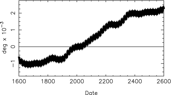
Figure 2. Pole Right Ascension change.
Download figure:
Standard image High-resolution image4.5. Gravity and Pole
Table 12 contains the Uranian system gravity parameters and their formal 1σ errors found by Jacobson et al. (1992) and those obtained from the current analysis. We were unable to estimate J6; consequently, we set its value to 0 in our dynamical model but took into account its a priori uncertainty when computing the statistics for the other parameters (i.e., it was treated as a consider parameter in the estimation process, see Bierman 1977). We use the system GM rather than the Uranus GM as our gravity parameter; given the magnitude of the satellite GMs the system is predominately the planet. The GMs of the Uranian system, Ariel, Umbriel, and Titania differ by several times the formal error, however, the differences are near the "adopted" errors quoted in Jacobson et al. (1992). We find smaller formal errors for Ariel and Umbriel, but larger errors for the system, Titania, and Oberon. Much of the difference is likely due to our revised data weighting, data processing procedures, and improved ephemerides. Moreover, we discovered that the Jacobson et al. (1992) analysis erroneously included a considerable amount of simultaneous two-way and three-way Voyager 2 Doppler. These effectively redundant data overweight the Doppler and produce lower formal errors. We removed the extraneous three-way from our fit. The remaining columns in Table 12 show the gravity results obtained from fits to various subsets of our data (J6 was a consider parameter in those fits). Table 13 summarizes the sets of parameters and the number in the set that we estimated when fitting each data subset; we estimated all of the parameters in the fit to all of data. Note that the large number of parameters in some sets, e.g., camera pointing angles, is a consequence of having separate parameters for differing time intervals (see sub Section 4.1).
Table 12. Uranus Gravity Parameters and Pole
| Parameter | Jacobson | Current | Astrometry | Voyager |
|---|---|---|---|---|
| et al. (1992) | Results | Only | Only | |
| GM (km3 s−2) | ||||
| System | 5794548.6 ± 1.5 | 5794556.4 ± 4.3 | 5795232.8 ± 625.1 | 5794566.1 ± 9.3 |
| Ariel | 90.3 ± 2.3 | 83.5 ± 1.4 | 68.2 ± 10.9 | 132.8 ± 10.4 |
| Umbriel | 78.2 ± 2.3 | 85.1 ± 1.9 | 99.4 ± 11.2 | 49.4 ± 17.8 |
| Titania | 235.3 ± 1.9 | 226.9 ± 4.1 | 224.4 ± 7.0 | 214.2 ± 9.2 |
| Oberon | 201.1 ± 1.8 | 205.3 ± 5.8 | 193.1 ± 10.1 | 201.1 ± 9.6 |
| Miranda | 4.4 ± 0.2 | 4.3 ± 0.2 | 4.0 ± 0.7 | 5.0 ± 0.3 |
| J2 (× 106) | 3513.2 ± 0.3a | 3510.7 ± 0.7 | 3606.2 ± 83.1 | 3595.0 ± 41.0 |
| J4 (× 106) | −31.8 ± 0.4a | −34.2 ± 1.3 | 716.0 ± 797.3 | −239.1 ± 177.1 |
| J6 (× 106) | 0.0 ± 1.0b | 0.0 ± 1.0b | 0.0 ± 1.0b | |
| α (deg) | 77.311 ± 0.010a | 77.310 ± 0.002 | 77.326 ± 0.018 | 77.691 ± 0.246 |
| δ (deg) | 15.174 ± 0.010a | 15.172 ± 0.002 | 15.157 ± 0.017 | 15.002 ± 0.718 |
| Parameter | Astrometry | Rings | Astrometry | Voyager |
| & Voyager | Only | & Rings | & Rings | |
| GM (km3 s−2) | ||||
| System | 5794564.0 ± 5.6 | 5794519.0 ± 3460.7 | 5795208.1 ± 623.8 | 5794574.6 ± 8.7 |
| Ariel | 78.8 ± 3.3 | 77.6 ± 4.3 | 93.5 ± 6.7 | |
| Umbriel | 89.6 ± 3.4 | 89.8 ± 5.2 | 111.1 ± 13.2 | |
| Titania | 225.6 ± 4.5 | 224.6 ± 7.0 | 220.1 ± 6.5 | |
| Oberon | 200.0 ± 6.3 | 194.0 ± 10.1 | 209.6 ± 9.3 | |
| Miranda | 4.1 ± 0.2 | 4.5 ± 0.5 | 4.4 ± 0.3 | |
| J2 (× 106) | 3520.3 ± 11.2 | 3510.5 ± 1.3 | 3510.3 ± 0.7 | 3510.5 ± 0.7 |
| J4 (× 106) | −47.3 ± 62.2 | −34.4 ± 1.3 | −34.4 ± 1.3 | −34.5 ± 1.3 |
| J6 (× 106) | 0.0 ± 1.0b | 0.0 ± 1.0b | 0.0 ± 1.0b | 0.0 ± 1.0b |
| α (deg) | 77.322 ± 0.011 | 77.310 ± 0.003 | 77.310 ± 0.002 | 77.309 ± 0.002 |
| δ (deg) | 15.174 ± 0.011 | 15.172 ± 0.002 | 15.172 ± 0.002 | 15.172 ± 0.003 |
Notes. The reference radius for the Uranus zonal harmonics is 25559 km. aFrom French et al. (1988). bNot estimated (see text).
Download table as: ASCIITypeset image
Table 13. Parameter Sets and the Number of Parameters Contained in the Set That Were Fit to Each Data Subset
| Parameter Set | Astrometry | Voyager | Astrometry |
|---|---|---|---|
| Only | Only | and Voyager | |
| Gravity and pole | 10 | 10 | 10 |
| Satellite states | 36 | 36 | 36 |
| Micrometer observation biases | 22 | 22 | |
| Absolute astrometry biases | 72 | 72 | |
| CCD observation orientation and scale | 198 | 198 | |
| Star position corrections | 4 | 4 | |
| Ring elements | |||
| Observatory time offsets | |||
| Spacecraft state | 6 | 6 | |
| RTG acceleration | 2 | 2 | |
| Spacecraft non-gravitational accel. | 542 | 542 | |
| Trajectory correction maneuver | 3 | 3 | |
| Impulsive maneuvers | 32 | 32 | |
| Tracking data ionosphere delays | 36 | 36 | |
| Range biases | 3 | 3 | |
| Quasar location | 2 | 2 | |
| Spacecraft camera pointing angles | 936 | 936 | |
| Imaging data phase corrections | 5 | 5 | |
| Parameter Set | Rings | Astrometry | Voyager |
| Only | & Rings | & Rings | |
| Gravity and pole | 10 | 10 | 10 |
| Satellite states | 36 | 36 | |
| Micrometer observation biases | 22 | ||
| Absolute astrometry biases | 72 | ||
| CCD observation orientation and scale | 198 | ||
| Star position corrections | 24 | 28 | 24 |
| Ring elements | 36 | 36 | 36 |
| Observatory time offsets | 10 | 10 | 10 |
| Spacecraft state | 6 | ||
| RTG acceleration | 2 | ||
| Spacecraft non-gravitational accel. | 542 | ||
| Trajectory correction maneuver | 3 | ||
| Impulsive maneuvers | 32 | ||
| Tracking data ionosphere delays | 36 | ||
| Range biases | 3 | ||
| Quasar location | 2 | ||
| Spacecraft camera pointing angles | 936 | ||
| Imaging data phase corrections | 5 | ||
Download table as: ASCIITypeset image
There are no resonances in the Uranian satellite system to enhance the determination of the satellite GMs from the effects of mutual perturbations on the satellite orbits. All that can be done is to observe the orbits' periapsis and nodal precession rates induced by those perturbations over an extended time period. The near-commensurability among Miranda, Ariel, and Umbriel does help a bit by adding a constraint on the product of the Ariel and Umbriel GMs. During the Voyager 2 Uranus encounter, tracking data was acquired only during the Uranus and Miranda close flybys. Consequently, the GMs of only those two bodies can be determined directly from the Doppler. The Uranus close flyby data also has some sensitivity to the Uranus J2 and pole orientation. The occultations of the elliptical inclined precessing rings are strongly sensitive to the orientation of the pole and the Uranus gravitational harmonics, slightly sensitive to the system GM, but totally insensitive to the satellite GMs.
From the fourth column of Table 12 we see that with our long arc of astrometry, we can obtain plausible estimates for the GMs, the J2, and the pole orientation, but the error in the system GM is large, and the J4 is indeterminate. It also turns out that the Ariel and Umbriel GMs are strongly correlated.
The results in the fifth column of the table confirm that the Voyager 2 data yield estimates of the system and Miranda GMs and the J2. The pole is weakly determined, and there is some sensitivity to J4. The estimates of GMs of the other four satellites are no better than with astrometry alone; it is actually the observations of the satellite motions with the imaging data that lead to these estimates. We find that the two zonal harmonics are moderately correlated, but the Ariel and Umbriel GMs are uncorrelated.
The combination of the astrometry and Voyager 2 data leads to a good determination of all of the parameters but J4. The two zonal harmonics are strongly correlated, the strong correlations remain between the Ariel and Umbriel GMs, and those GMs are now moderately correlated with J2.
Using only the ring occultations, we get a poor estimate of the system GM (the precession rates depend upon the Uranus mass as well as the zonal harmonics) but excellent estimates of the zonal harmonics and pole. The J2 and J4 are uncorrelated, but J2 is correlated with the system GM. We found that the effect of the J6 uncertainty is to approximately double the error in J4.
When the occultations are combined with the astrometry, a surprising good determination of the Ariel and Umbriel GMs occurs, but the system, Titania, Oberon, and Miranda GM estimates are nearly unchanged from the astrometry only case. The correlation between the system GM and J2 disappears, but the two zonal harmonics become strongly correlated. The Ariel and Umbriel GMs continue to be correlated.
Adding the occultations to the Voyager 2 data has an interesting effect on the Ariel and Umbriel GMs, namely, a significant decrease in that of Ariel and increase in that of Umbriel. Both of those GMs are still uncorrelated, and the zonal harmonics continue to be strongly correlated.
When all of the data are used the correlation between the harmonics becomes 0.978 and between the Ariel and Umbriel GMs is 0.810. There are no other correlations of significance amongst the gravity and pole parameters.
5. CONCLUDING REMARKS
In this article we report the results of a comprehensive analysis of the orbits of the main Uranian satellites and rings and of the gravity field of the Uranian system. In determining the satellite orbits, we extended the observational data arc used in previously published orbits to include astrometry through the end of 2013. We also included the mutual events observed in 2007. For the ring orbits we extended the data arc to the Earth-based observations made in 1992. Our gravity field parameter determination required the combination of the satellite astrometry, ring occultations, and radiometric tracking of the Voyager 2 spacecraft during its passage through the Uranian system. We found that an accurate estimate of the Uranian system GM, i.e., the planet GM, could only be made from the Voyager 2 data. Adding the astrometry yielded the GMs of the satellites, and adding the occultations determined the zonal harmonics and pole direction. However, we also found consistent but lower accuracy values of the harmonics and pole from just the combination of the astrometry and Voyager 2 data.
Our satellite and ring orbits are well determined. Additional astrometry and occultations in the coming decades should provide moderate improvement. With respect to the gravity field, problems remain. The GMs of Ariel and Umbriel are correlated as are the Uranus zonal harmonics. We believe that more Earth-based astrometry will not break these correlations. However, additional ring occultation measurements may moderately improve the determination of J2, J4, and the pole orientation. Any significant improvement will require another spacecraft mission to the system. We recommend a mission similar to Galileo or Cassini, i.e., an orbiter with close satellite flybys. The orbiter must have low altitude Uranus periapsis passages for the tracking data to be sensitive to the Uranus gravitational harmonics and pole direction.
The Uranus pole precession rate is about 1.3 mas yr−1 which is too small to be detected with the current data set (we were unable to determine it within the context of this analysis), but it may measurable in the future with a decade or more of high precision, ≈1 mas, absolute satellite astrometry. With the precession known we can infer the Uranus moment of inertia, γ.
Ephemerides for all of the satellites are available electronically from the JPL Horizons online solar system data and ephemeris computation service1 and from NASA's Navigation and Ancillary Information Facility2. The ephemeris designation is URA111.
The research described in this publication was carried out at the Jet Propulsion Laboratory, California Institute of Technology, under a contract with the National Aeronautics and Space Administration. We wish to thank Richard French for his helpful discussions concerning the ring orbit model and occultation data processing.
APPENDIX A: RING MODEL
We define a ring plane coordinate system in terms of equinoctial coordinates (Broucke & Cefola 1972); the unit vectors along the coordinate axes are
where p = tan (I/2)sin Ω, q = tan (I/2)cos Ω, I is the inclination of the ring plane to the planet equator, and Ω is the node of the ring plane on the planet equator; Ω is measured from the intersection of the planet equator and the ICRF reference equator. The unit vector  is the pole of the ring plane. The rotation of an arbitrary vector x between planet equatorial and ring plane coordinates is

 is the standard rotation of a vector by angle ϕ about coordinate axis j. The ring plane pole and the other ring plane coordinate axes in the ICRF system are

where α and δ are the ICRF right ascension and declination of the planet pole. If the ICRF position of a ring particle is  , and we define the direction
  then
then

where λ is the true longitude measured from the  axis. By construction λ is equal to the "broken" angle v + ϖ; v is the true anomaly measured from periapsis, and ϖ is the longitude of periapsis.
For an elliptical ring, the radial position in the ring plane is
where a is semi-major axis of the ring, e is eccentricity of the ring, h is e sin ϖ, and k is e cos ϖ. If we allow the ring node and periapsis to precess, i.e.,

where t is time from epoch, we find
with h0, k0, p0, snd q0 being the values of h, k, p, and q at epoch t = 0.
The longitude rates are computed from the secular rate expressions from Borderies-Rappaport & Longaretti (1994) augmented with the perturbations due to external satellites based on the secular perturbations in Brouwer & Clemence (1961):
where μ0 is the planet GM, μi is the GM of satellite i, Jn is n'th zonal gravity harmonic of the planet, R is the planet's equatorial radius, γi = a(1 + 1/2e2)/ai, ai is the orbital radius of satellite i, and  is the j'th Laplace coefficient of degree s; it is function of γi.
APPENDIX B: POLE MODEL
The equations of the rotational motion of Uranus torqued by the Sun and five satellites are
where H0 is the angular momentum of Uranus,  is the Uranus pole vector, R is the Uranus's equatorial radius, J2 is Uranus's second zonal gravity harmonic, μ☉ is the GM of the Sun, m0 is the mass of Uranus,
  is the distance of Uranus from the Sun,
  is the direction vector from Uranus to the Sun, μj is the GM of satellite j,
  is the distance of satellite j from Uranus,
  is the direction vector from Uranus to satellite j.
If we average over the orbital motion of the Sun and satellites about Uranus, we find that
where  is the unit vector normal to the Uranus orbit or to the Uranus centered orbit of satellite j. Consequently, the long term Uranus rotational motion is described by
Assuming that the angular momentum of Uranus is dominated by its spin angular momentum we have
with s being the planet rotation rate and γ its axial moment of inertia factor. For a constant rotation rate,
Because of the orthogonality of the vectors  , we find
We numerically integrated Equations (B6–B7) over the 1000 yr period from 1600 to 2600. The solar and satellite masses, distances, and orbit normals were taken from the ephemerides. We set J2 = 3510.7 × 10−6, γ = 0.2269 (Hubbard & Marley 1989), and s = 501.1600928 deg day−1 (Desch et al. 1986). The initial pole orientation angles (at J2000) were α = 77309980 and δ = 15172395. The Figures 2 and 3 display the change in the right ascension and declination over the 1000 yr period. We obtained the following analytical representation of the orientation angles by fitting a trigonometric series to the integration.
with
where T is Julian centuries and d is days from J2000; the added the S5 term forces the series to sum to 0 at epoch. The series can be simplified by adding the S5 term to the constant term.

Figure 3. Pole declination change.
Download figure:
Standard image High-resolution image
Footnotes
- *
Government sponsorship acknowledged.
- 1
- 2