


ABSTRACT
On 2005 November 27 (day 331), the Visual and Infrared Mapping Spectrometer instrument onboard the Cassini spacecraft obtained high signal-to-noise, spatially resolved measurements of Enceladus' particle plume. These data are processed to obtain spectra of the plume at a range of altitudes between 50 and 300 km from the surface. These spectra show that the particulate component of the plume consists primarily of fine-grained water ice. The spectral data are used to derive profiles of particle densities versus height, which are in turn converted into measurements of the velocity distribution of particles launched from the surface between 80 and 160 m s−1 (that is, between one-third and two-thirds of the escape speed). These calculations indicate that particles with radii of 1 μm are approximately equally likely to have launch speeds anywhere between 80 and 160 m s−1, while particles with radii of 2 and 3 μm have progressively steeper velocity distributions. These findings should constrain models of particle production and acceleration within Enceladus.
Export citation and abstract BibTeX RIS
1. INTRODUCTION
Saturn's moon Enceladus vents material from its interior to high above its surface, producing a plume of gas and particulate matter that extends hundreds of kilometers above the moon's surface to supply water molecules to the inner magnetosphere and ice grains to the extensive E ring. Various instruments onboard the Cassini spacecraft have reported measurements of the heat flux from the surface (Spencer et al. 2006), the dust and gas distribution in this plume (Porco et al. 2006; Hansen et al. 2006; Spahn et al. 2006; Waite et al. 2006; Spitale & Porco 2007; Tian et al. 2007), and its interactions with the moon's surface and the local plasma (Dougherty et al. 2006; Brown et al. 2006; Tokar et al. 2006; Jones et al. 2006; Jaumann et al. 2008; Newman et al. 2008). However, there is still considerable debate regarding many aspects of this phenomenon. For example, there are several different models for how the gas and solids in the plume are produced and accelerated, including boiling liquids (Porco et al. 2006) and degassing clathrates (Kieffer et al. 2006).
In this paper, we analyze spatially resolved spectra of the particulate component of the plume obtained by Cassini's Visual and Infrared Mapping Spectrometer (VIMS). These data reveal that the particulate matter in the plume is composed largely of small grains of water ice. Furthermore, variations in the spectrum of the plume with altitude can be translated into information about the velocity distribution of particles launched from the surface, which should constrain models for the acceleration of solids within the moon (Schmidt et al. 2008).
Section 2 summarizes the VIMS observations of the plume and how they are processed to produce integrated spectra of the plume at a variety of altitudes above the surface of Enceladus. Section 3 discusses how the velocity distribution of particles launched from the surface determines the shape of these spectra. Sections 4 and 5 describe in detail how the spectra are used to constrain the particle size distribution at different altitudes and how profiles of the particle densities versus altitude are transformed into velocity distribution profiles. The results of our analysis are discussed in Section 6.
2. VIMS PLUME DATA
VIMS is described in detail in Brown et al. (2004). Briefly, this instrument acquires spectra at 352 wavelengths between 0.35 and 5.2 μm for an array of up to 64 × 64 spatial pixels to produce a map of the spectral properties in a given scene known as a "cube." Two separate channels measure the visual and infrared (IR) components of the spectra. In this paper, we will focus exclusively on data from the IR channel, which measures spectra at 256 points between 0.85 and 5.1 μm with a typical spectral resolution of 0.016 μm. For the data considered here, the spatial resolution of the VIMS IR channel was 0.25 × 0.5 mrad.
On 2005 November 27 (day 331), Cassini flew by Enceladus with a closest approach distance of roughly 108,000 km from the moon's center. After closest approach, the moon was observed by the remote-sensing instruments at a phase angle of 161°. During this time, the VIMS instrument obtained 109 cubes, but for various reasons many of these cubes are excluded from this analysis. The last 24 cubes of the sequence were obtained with Enceladus either in close proximity to the rings or in front of Saturn. The first 38 cubes in the sequence were excluded because the cubes did not capture a sufficiently large region around Enceladus to provide much useful data on the plume. Another 14 cubes were obtained while the spacecraft rotated about the camera axis, which would greatly complicate this analysis. Finally, we exclude eight cubes with IR exposure times per pixel less than 100 ms as the signal-to-noise ratios (S/Ns) in these data were generally poor.
The remaining 25 cubes included in this analysis are tabulated in Table 1. All have the plume oriented in the same direction in the image plane, such that the IR channel had higher resolution along the vertical axis of the plume (0.25 mrad) than horizontally perpendicular to the plume axis (0.5 mrad). The effective vertical resolution of these cubes was between 30 and 40 km.
Table 1. Data Files Used in This Analysis
| Filename | Image Midtime | Image Size | IR Exposure (ms) | Range (km) | Phase | Group |
|---|---|---|---|---|---|---|
| V1511793703 | 2005-331T14:14 | 40 × 30 | 180 | 126,200 | 160 6 6 |
1 |
| V1511794087 | 2005-331T14:26 | 40 × 30 | 640 | 126,900 | 1607 |
1 |
| V1511794976 | 2005-331T14:39 | 40 × 30 | 480 | 128,400 | 1609 |
1 |
| V1511795691 | 2005-331T14:48 | 40 × 30 | 180 | 129,600 | 1611 |
1 |
| V1511795992 | 2005-331T14:56 | 40 × 30 | 480 | 130,100 | 1611 |
1 |
| V1511796659 | 2005-331T15:09 | 40 × 30 | 640 | 131,200 | 1612 |
1 |
| V1511797548 | 2005-331T15:20 | 40 × 30 | 320 | 132,600 | 1613 |
1 |
| V1511798077 | 2005-331T15:28 | 40 × 30 | 180 | 133,500 | 1613 |
1 |
| V1511798376 | 2005-331T15:38 | 40 × 30 | 640 | 134,000 | 1613 |
1 |
| V1511799265 | 2005-331T15:47 | 40 × 30 | 110 | 135,500 | 1613 |
1 |
| V1511799464 | 2005-331T15:52 | 40 × 30 | 280 | 135,800 | 1613 |
1 |
| V1511799891 | 2005-331T15:58 | 40 × 30 | 180 | 136,600 | 1613 |
1 |
| V1511800181 | 2005-331T16:05 | 27 × 27 | 640 | 137,100 | 1613 |
2 |
| V1511800741 | 2005-331T16:14 | 27 × 27 | 640 | 138,000 | 1613 |
2 |
| V1511801493 | 2005-331T16:28 | 30 × 30 | 620 | 139,400 | 1613 |
2 |
| V1511802247 | 2005-331T16:40 | 30 × 30 | 620 | 140,800 | 1613 |
2 |
| V1511803001 | 2005-331T16:53 | 30 × 30 | 620 | 142,300 | 1613 |
2 |
| V1511807379 | 2005-331T18:04 | 30 × 30 | 400 | 152,800 | 1614 |
3 |
| V1511807805 | 2005-331T18:13 | 30 × 30 | 640 | 154,100 | 1614 |
3 |
| V1511808707 | 2005-331T18:25 | 24 × 30 | 320 | 156,900 | 1613 |
3 |
| V1511809066 | 2005-331T18:31 | 30 × 30 | 180 | 158,200 | 1613 |
3 |
| V1511809439 | 2005-331T18:37 | 30 × 30 | 180 | 159,500 | 1613 |
3 |
| V1511809666 | 2005-331T18:41 | 24 × 30 | 220 | 160,300 | 1612 |
3 |
| V1511809910 | 2005-331T18:46 | 30 × 30 | 400 | 161,200 | 1612 |
3 |
| V1511810387 | 2005-331T18:51 | 24 × 30 | 400 | 163,000 | 1612 |
3 |
Download table as: ASCIITypeset image
All the cubes were calibrated and processed using the standard pipelines to remove dark currents and to convert raw data numbers into the standard measure of reflectance I/F, which is unity for a perfect Lambert surface oriented perpendicular to the incident light (McCord et al. 2004). The specific calibration file used in this analysis was RC17. The S/N on the plume in individual cubes is low, so to obtain useful spectral data on the plume we combine measurements from as many pixels as possible. The available cubes are divided into three groups (numbered 1–3 in Table 1) based on observation time so that within each group the range to Enceladus changes by less than 10%. For each set of cubes, we co-add the data at each wavelength to produce a "combined cube" with higher signal-to-noise. Differences in exposure times among the different cubes in each set were accounted for by computing the standard deviation among 36 pixels in one corner of the image plane that contained only the (spatially featureless) background sky signal. These standard deviations were used to compute a wavelength-dependent weight for each cube and error bar per pixel for the combined cubes. This was considered a more reliable method of estimating uncertainties than using the exposure durations, which would not directly provide estimates in the relative uncertainty at different wavelengths.
Note that because each combined cube is composed of cubes taken over a finite time interval while the spacecraft was moving away from Enceladus, we expect some smearing in the combined images. While this smearing could be removed or reduced by resampling individual cubes to a common overresolved coordinate grid, given the low S/N in individual cubes and the gradual trends observed in the combined spectra (see below), we have elected not to implement this refinement to the analysis at the present time.
Figure 1 shows images based on three spectral channels of these combined cubes. In each case, the dark disk of Enceladus can be seen silhouetted against the E ring, as well as the bright southern limb of the moon. The plume can be seen extending from the South Pole toward the edge of the frame. Note that the size of the disk changes significantly between the three cubes as the spacecraft moved away from Enceladus; the mean distances to the moon's center for these three cubes are 131,700 km, 139,500 km, and 158,300 km, respectively.
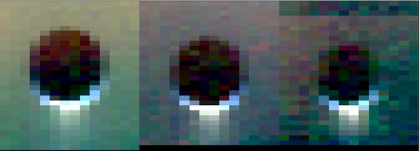
Figure 1. Images based on the combined cubes used for this analysis. Each of the three panels corresponds to a subset of the pixels from the combined cubes 1, 2, and 3 from left to right. These cubes were obtained at mean ranges of 131,700, 139,500, and 158,300 km, respectively. The red, green, and blue colors correspond to 2.37, 1.70, and 0.88 μm, respectively. The dark disk of Enceladus is silhouetted against the background E ring, while the images have been rotated by 90° for display purposes to position the lit southern crescent and plume at the bottom of the images.
Download figure:
Standard image High-resolution imageThese images demonstrate that the core of the plume is only a pixel or two wide, so VIMS is unable to resolve horizontal structures in the plume. We, therefore, integrate the plume signal horizontally to obtain higher S/N plume spectra at varying heights above the surface. For each row in each combined cube, the average brightness between 0.88 and 1.21 μm (where the S/N is reasonably high at all observed altitudes) is fit to a Gaussian in order to estimate the width of the plume and the location of peak brightness within the row. Then, for each wavelength, a quadratic background is fit to the data more than ±3 Gaussian widths from the plume center and the signal excess above this background level within ±3 Gaussian widths of the plume center is summed to produce an integrated measurement of the plume reflectivity known as the "equivalent width":
Note that because we integrate over horizontal rows of pixels, the spectra derived here do not correspond precisely to a single altitude above the surface of the moon. However, given the narrowness of the plume and the resolution of the VIMS data, these horizontally integrated spectra should closely approximate the spectra integrated over a circle at a fixed radius from the moon's center. We, therefore, compute an effective altitude for each integrated spectrum based on the minimum altitude of the row above the limb of Enceladus. The location of the limb in the field was determined by finding the brightest pixel at short wavelengths in a slice of the image bisecting the moon and the plume. The effective minimum altitude for each row i from the edge of the frame was then computed using the following formula (note we take the southernmost row to correspond to i = 0):

where "Range" is the distance between the spacecraft and the moon (131,700 km, 139,500 km, and 158,300 km for combined cubes 1, 2, and 3, respectively) and jlimb is the pixel number of the limb, which is taken to be 7 for combined cubes 2 and 3, and 8.5 for combined cube 1 (because rows 8 and 9 are comparably bright in this cube). Note that a half-pixel uncertainty in the pointing will correspond to a 15–20 km systematic uncertainty in the altitudes.
Figure 2 shows some sample spectra of the plume at four altitudes derived from combined cube 1 (all the plume spectra derived from this analysis are presented in the Appendix). The most obvious feature in all of the plume spectra is a dip near 3 μm. This corresponds to the strongest water ice absorption band in the near-IR and demonstrates that the particles in the plume are composed primarily of water ice. No narrow features have been identified in these spectra that could be attributed to non-water-ice contaminants in the plume at this time. Furthermore, thermal emission from the plume particles—assuming they are less than 500 K—would produce a steeply rising spectrum at long wavelengths. No such rise can be seen in the data, so we will assume here that the observed light is entirely due to scattering of solar radiation by ice-rich particles.
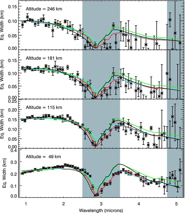
Figure 2. Sample spectra of the plume derived from four altitudes or rows in the combined cube 1. The data are shown as the points with error bars. To improve S/Ns, these spectra have been rebinned by a factor of 4 in wavelength. All these spectra show a clear absorption band at 3 μm due to water ice. Outside this band, there are variations in the overall slope of the spectra that are sensitive to the particle size distribution in the plume. The black curves are the best-fit model spectra derived using the procedures discussed in the text, while the colored curves are scaled spectra for the same best-fit size distributions computed using Mie theory for spheres (red) and for irregular shape models 3 (green) and 5 (blue) from Pollack & Cuzzi (1980). The shaded regions are not included in this fit.
Download figure:
Standard image High-resolution imageOutside of the 3 μm band, the spectra are rather featureless, but there are systematic variations in spectral slopes with wavelength and altitude that can potentially constrain the distribution and dynamics of the plume particles. In particular, comparing the brightness measurements over a range of wavelengths should constrain the particle size distribution at different altitudes in the plume, and particle density variations with altitude can be translated into estimates of the velocity distribution of the particles launched from the surface. The remainder of this paper describes the techniques we have used to derive information about the velocity distribution of the particles in the plume from the spectral data.
3. BACKGROUND: HOW THE VELOCITY DISTRIBUTION DETERMINES PLUME SPECTRA
Before discussing the specific methods we have applied to retrieve velocity information from spectral data, it is useful to first describe how the velocity distribution function of the particles at the surface determines the spectral properties of the plume. This will both introduce the notation system used in this paper and clarify several assumptions behind the analysis.
3.1. From Surface Velocity Distribution to Plume Density
Since VIMS does not resolve individual jets, these data can only constrain the total rate of particles launched from the surface ∫f(vo, s)dvods, where vo is the radial component of the velocity at the moon's surface and s is the size (radius) of a particle. The function f specifies the distribution of particle velocities as a function of particle size. The primary goal of this analysis is to constrain f because this function can, in principle, be compared with predictions from various physical models for the origin and acceleration of the particles (e.g., Schmidt et al. 2008).
Given the low optical depth of the plume, it is reasonable to assume that after the particles leave the surface they follow purely ballistic trajectories. In this case, the density of the plume versus height above the surface is determined entirely by f. Furthermore, since the VIMS data discussed here only detect the plume up to altitudes of 300 km above the moon's surface (or 550 km from the moon's center), which is well inside Enceladus' Hill sphere radius of 1440 km, we can assume that the moon's gravity dominates the particle trajectories. Conservation of energy then requires that the following quantity is a constant along any particle's trajectory:
where r is the particle's distance from the moon's center, v(r) is the radial component of the particle's velocity, G is Newton's constant, and ME is the mass of Enceladus (GME = 7.21 km3 s−2 from Jacobson et al. 2006 and Rappaport et al. 2007). We can, therefore, relate the radial component of the particle's velocity at a given radius v(r) to the radial component of the particle's velocity when it is launched from the moon's surface vo:
where ro = 248 km is the radius of Enceladus (Thomas et al. 2007) and ΔΦ(r) is the difference in gravitational potential between ro and r.
Provided the plume is nearly in a steady state, then there is a straightforward relationship between f and the density of plume particles as a function of height. First, consider particles launched from the surface with an initial speed greater than the escape speed  . When the plume is in a steady state, the flux of particles through a given surface at a distance r from the moon's center is independent of r. Thus, for vo > vesc, we can define
where descape(r, s) is the differential number density of escaping particles of size s at a radius r. Note this is the differential number density integrated over the surface of a spherical shell, so d(r, s)ds has units of length−1 and d(r,s) has units of length−2.
Particles with vo < vesc, by contrast, will reach a maximum altitude where v(r)2 = v2o − 2ΔΦ(r) = 0 and then fall back to the surface. Thus, at a given r only particles launched with a velocity vo greater than the critical velocity  will contribute to this population, and the integrated density distribution d at a given r of trapped particles will be
the factor of 2 in this expression arises because the particles pass through the given radius twice as they rise and fall through the plume.
The total density in the plume is the sum of these two terms:
3.2. From Plume Density Distributions to Spectra
Given the integrated density of particles at a given height, the brightness of the plume as a function of wavelength can be computed using the appropriate scattering theory. Say the particles are illuminated by flux πF of radiation with wavelength λ. The power scattered by an individual particle per unit solid angle is described by the function dP/dΩ (note in this context P indicates power, not phase function), which depends on F, λ, the scattering angle (180° − phase angle) θ, the radius of the particle s, the optical properties of the particles, etc. A variety of sophisticated models have been developed over the years to calculate the light scattering properties of small grains (e.g., van de Hulst 1957). However, as discussed in detail in Section 4.1, simpler diffraction-based analytical calculations can also provide useful estimates of dP/dΩ in certain cases.
Regardless of how it is calculated, once dP/dΩ is determined for particles of range of different sizes s, the reflectivity of a collection of particles can be evaluated by integrating dP/dΩ over the appropriate size distribution. For example, the reflectivity of a region filled with a population of particles described by the differential size distribution n(s)ds at a given wavelength will be
where ∫n(s)dl is the particle size distribution integrated along the line of sight. Similarly, the equivalent width of the plume (assuming it is sufficiently collimated) is given by
where we identify d as the integral of n(s) along the line of sight and horizontally across the plume (given by Equation 7) and we again assume that the observed light is dominated by radiation scattered from particles near the minimum altitude along the line of sight.
4. DERIVING PARTICLE SIZE DISTRIBUTIONS FROM SPECTRA
Provided that the plume is sufficiently well collimated the integrated measurements of the plume spectrum computed in Section 2 and illustrated in Figure 2 will be good estimates of the total integrated reflectivity over spherical shells E(r, λ). These measurements of E, therefore, can constrain the density distributions d(r, s) of particles at different heights, and in turn these estimates of d(r, s) can be converted into estimates of the particle velocity distributions at the moon's surface, f(vo, s).
Deriving robust constraints on the particle size distribution from spectrophotometry is challenging because a single particle scatters light in a particular direction over a range of wavelengths. Previous studies of low-optical-depth populations of small dust grains in the solar system have compared the spectrophotometric data to either the predictions for a few size distributions derived from physical models (e.g., Throop & Esposito 1998), or to restricted classes of size distributions with a limited number of free parameters, such as power laws or Hansen–Hovenier distributions (e.g., Showalter et al. 1991). Neither of these approaches is appropriate in this case. At present, there is no single favored physical model for the origin and acceleration of the plume particles, so a fit to the currently available models may not be particularly useful for future research. Furthermore, preliminary investigations revealed that simple size distributions like power laws are unable to reproduce the relatively flat spectral slopes between 1 and 2 μm and the ratio in brightness between 2 and 4 μm. We have, therefore, elected to compare the spectra to a more generic suite of models.
4.1. Defining of the Parameter Space
A completely generic set of model size distributions can be generated by specifying the particle density distribution at a discrete set of particle sizes si, and then interpolating between these values to all values of s. In principle, an infinite number of si are needed to specify a completely arbitrary size distribution. In practice, however, the available spectral data can only constrain the particle size distribution over a limited range of s and cannot resolve infinitely sharp features in the size distribution. Thus, there is an optimal set of si that contains the smallest number of parameters needed to reproduce any observed spectrum.
In this case, we are fortunate because the plume data were obtained at such high phase angles that the observed light is predominantly due to diffraction around individual particles. Elementary Fraunhofer diffraction theory can, therefore, provide insights into the connection between the measured spectra and the particle size distribution and help us find the optimal choice of si.
Consider a circular conducting disk of radius s illuminated by flux πF of radiation with wavelength λ. The power per unit solid angle scattered by this disk is described by the following function (slightly modified from Equation 9.168 in Jackson 1975):

where k = 2π/λ, θ is the scattering angle (180° − the phase angle), and J1(z) is a Bessel function of z.
While the above equation applies to conducting obstacles, a similar expression can be used to approximate the diffracted signal from dielectric particles like those in the plume, accounting for the (possibly wavelength-dependent) index of refraction of the material. Mie theory calculations show that to first order the optical properties of the dielectric do not strongly affect the shape of this part of the phase function (i.e., the θ-dependent terms in dP/dΩ, see Fymat & Mease 1981). Thus, to first order, we only need to multiply the above expression by a scaling factor that is independent of scattering angle but does depend on wavelength. It turns out that the most elementary way to do this is to exploit the optical theorem, which relates the imaginary part of the forward-scattered signal to the total cross section of the obstruction (see Jackson 1975, p. 453; also van de Hulst 1957, pp. 30–36): this means that the desired scaling factor can be derived directly from the so-called extinction factor Qext, which is defined as the ratio of the total cross section of the particle to its geometrical cross section and can be computed from Mie theory. For perfect conductors Qext = 2, but in general Qext is a function of ks and the index of refraction mr + imi of the object (van de Hulst 1957, p. 179):
where tan β = mi/(mr − 1) and ρ = 2ks(mr − 1). This function declines to zero as ks approaches zero and asymptotes to 2 when ks > >1.
In the limit where the Mie scattering amplitude function S is purely real, the optical theorem indicates that the scattering law for a dielectric can be approximated as the above expression for a conductor scaled by Q2ext/4 (Fymat & Mease 1981):
Thus, the equivalent width of the plume is given by (from Equation 9)
Figure 3 compares the spectra derived using this method with the results of full Mie calculations for spheres and irregular particles computed using the techniques outlined in Pollack & Cuzzi (1980) and Showalter et al. (1992) for the case of pure ice grains with d(r, s) ∝ s−3 and s−4 viewed at a scattering angle θ = 20°. The spectra are scaled to match at short wavelengths for clarity. If the simple model yielded spectra with the same shape as the Mie calculations, the fractional difference would be constant. This is approximately true outside of the 3 μm band, which indicates that the simple model can adequately approximate the shape of the spectrum in these regions. However, in the vicinity of the strong ice band, the fractional differences change rapidly. This is because the large imaginary component of the refractive index causes the assumption that S is purely real to be violated. Note that for the irregular particle models (which are better fits to the observed spectra on account of their weaker 1.5 and 2 μm ice bands), the simple model agrees with the more exact calculations to within 50% everywhere outside of 2.5–3.5 μm, which should be sufficient for the purposes of this paper.
Figure 3. Comparison between the spectra for s−3 (top) and s−4 (bottom) particle size distributions viewed at a scattering angle of 20° (phase angle of 160°) calculated using the simple Fraunhofer diffraction model with the results of full Mie calculations for spheres and for two irregular particle models (Numbers 3 "cubes" and 5 "plates") of Pollack & Cuzzi (1980). The upper part of each plot shows the scaled spectra, while the bottom part shows the fractional difference between the simple model and the full Mie calculations.
Download figure:
Standard image High-resolution imageGiven this analytical approximation of particles' scattering properties does roughly reproduce numerical calculations, we can now use Equation (13) to determine the best range and spacing of si as a basis for a generic suite of particle size distributions. The Bessel function J21(kssin θ) has its tallest peak where kssin θ ≃ 2, which at phase angles of 160° (θ ≃ 20°), corresponds to s/λ ≃ 1. Furthermore, outside of the strong 3 μm absorption feature, water ice has a real index of refraction of approximately 1.3, which means that Qext(ks) peaks where ks ≃ 6, which also corresponds to s/λ ≃ 1. Thus, for this particular viewing geometry, particles of a size s are most efficient at scattering radiation into the instrument if the radiation's wavelength is comparable to s.
While this result indicates that there could be a relatively direct mapping from observed wavelength to particle size, such a simple result will only occur if we place certain constraints on the overall slope of the size distribution. These constraints are necessary because in addition to the primary peak at kssin θ ≃ 2, the Bessel function has secondary peaks at other values of kssin θ, which correspond to locations where s/λ = 2.8, 4.3, .... Thus, radiation with a wavelength λ could be efficiently scattered by particles of size λ, 2.8λ, 4.3λ, etc. Only if the size distribution is sufficiently steep, and the larger particles sufficiently rare, can we neglect the contribution of larger particles to the scattered light at a given wavelength. Fortunately, this condition does not place a very restrictive constraint on the particle size distribution, since even with a d(s) as shallow as s−2 the peak at s/λ = 2.8 is 6 times lower than the peak at s/λ = 1. We, therefore, expect that this condition will be satisfied everywhere in the plume.
If wavelength translates directly into particle size, then the VIMS IR spectra will primarily be sensitive to the particle size distribution in the 1–5 μm range. Furthermore, our ability to resolve structures in the size distribution will be limited by the finite width of the peak in the function J21(kssin θ)Q2ext(ks), which has a full width at half-maximum of approximately 0.7 in s/λ. Based on these considerations, we determined that interpolating a size distribution based on the specified densities at si = 0, 1, 2, 3, 4, and 5 μm would be sufficient for this analysis (the 0 and 5 μm values are used to provide well-defined endpoints for the interpolation). Note that while the evenly spaced si values used here are a reasonable choice, a slightly more optimal spacing would have the ratio of adjacent values si be a value specified by the width of the peak.
With the si selected, the next step is to determine the array of density values to assign to the si that will yield a reasonably complete suite of models. Here it is important to note that in the limit where the index of refraction is constant with wavelength, Equation (13) indicates that if d ∝ s−3 then the integrated reflectivity is independent of wavelength. This means the variations in the brightness level across the VIMS IR band measure deviations from this simple power-law form. The size distributions used in this analysis therefore all have the form d = C(s, si, ci)s−3, where C(s, si, ci) is a function that varies between 0 and 1. C(s, si, ci) is calculated by assigning a set of values ci to the selected particle sizes si = [0, 1, 2, 3, 4, 5] μm; interpolating between these discrete points to all other particle sizes s; and finally smoothing the size distribution with a moving boxcar average with a smoothing length equal to 1 μm. For this analysis, we computed size distributions for all possible combinations of ci where each ci could have any of the values 0, 0.25, 0.5, 0.75, or 1. This yielded a total of 15,625 (56) model size distributions.
4.2. Computing of the Model Spectra
In principle, we could calculate the spectrum for each of the 15,625 different size distributions using numerical Mie scattering or physical optics codes. However, the number of models involved makes this task computationally intensive. In this paper, we will instead approximate the spectra using Equation (13), which has the advantage of being faster to compute. While such an approximate method may affect the estimates of the particle size distribution somewhat, we expect that any errors introduced by this simplification will be comparable to uncertainties associated with the particles' shape and composition. For example, Figure 3 indicates that the shapes of the spectra derived with the analytic calculation differ from those of the proper numerical methods by of order 50%, which is comparable to the differences among models with different assumed particle shapes. To further verify the validity of this approach, we also compute spectra for the various best-fit size distributions obtained below using both the above approximate analytic theory and numerical scattering codes for Mie spheres and irregular particle models (see below).
For the purposes of this analysis, we assume the index of refraction values for water ice to evaluate Qext (provided by D. P. Cruikshank). This is reasonable, given that E-ring particles are known to be largely water ice (Postberg et al. 2008) and no spectral features beyond the strongest water ice band are apparent in the spectra. If any contaminants are present, they would therefore probably only affect the overall albedo of the particles, which will change the overall normalization of the density distributions, but not the trends with height. Similarly, the use of Equation (13) to approximate the scattering properties of the particles may also affect the density estimates, but should not have a large effect on the shape of the density profiles versus height.
4.3. Determining the Best-fit Model Spectrum
To determine which of the model particle size distributions best reproduces the observed spectra at various locations in the plume, each observed spectrum is compared to the complete array of model spectra. First, all the model spectra are renormalized so that they produce the same mean flux between 0.88 and 1.53 μm as the observed data, and the particle size distributions scaled appropriately. The goodness of fit of the observed shape of the spectra to the normalized models is then evaluated using χ2 statistics. These χ2 statistics are computed excluding the data from spectral channels associated with the filter gaps and known hot pixels, as well as the channels beyond 4.75 μm because of their extremely low S/N. We also exclude the data between 2.5 and 3.5 μm because our simplistic models do not reproduce the observed spectra well here (see Section 4.1). In total, 162 of the original 256 spectral channels are used to compute the χ2 statistics.
The reduced χ2 statistics for even the best-fit models are poor (typically around 5). This is probably not due to a deficiency in the models, but instead because the primary data reduction underestimates the error bars on the spectra. As can be seen in Figure 2, the scatter among nearby data points in a single spectrum is often larger than the error bars, so no smooth curve can fit these data well. The reasons for this are still not fully understood, but it may be due to slight offsets between spectral channels induced by the incomplete background subtraction. In spite of this issue, the χ2 statistics still provide a useful measure of how well the various models fit the data relative to one another, and the best-fit models should still be the ones with the smallest χ2.
In general, the above calculations do not produce a single uniquely favored model, but instead yield multiple models with comparably low values for χ2. This is partially because there are some redundancies in the array of models (i.e., ci = [0.5, 0.5, 0.5, 0, 0, 0] and [1, 1, 1, 0, 0, 0] will produce the same normalized spectrum) and the sampling of model size distributions is relatively coarse (so that the true best-fit model probably lies between some of the calculated models). However, we also find that models with similar densities between 1 and 4 μm but radically different densities below 1 μm and above 4 μm have roughly the same χ2 statistics. This should not be surprising, given the above arguments that the data would not be very sensitive to these regions of the size distribution. Thus, to prevent these outlying regions of particle size distribution from having an undue affect on the overall fit, we impose a constraint that the ci values for 0 and 5 μm must be less than or equal to those for 1 and 4 μm, respectively. After applying this constraint, a single estimate for the size distribution responsible for generating the observed spectrum is computed as the weighted mean of the individual models with the lowest χ2 statistics. To obtain the weights for the models, the χ2 statistics are first rescaled so that the best-fit model has a reduced χ2 = 1 (this amounts to rescaling the error bars by a fixed factor). The probability to exceed the rescaled χ2 then provides the appropriate weight for each model.
4.4. Results of the Spectral Fits
Figure 2 (as well as the figures in the
Figure 4 illustrates the size distributions derived from the integrated spectra for the three different combined cubes. We caution against taking these size distributions too literally, given the approximations used in computing the model spectra, which are only good to within 50%. However, we do wish to point out that all three cubes show similar features and all show consistent and repeatable trends in the size distributions with altitude. This provides some evidence that the above fitting procedures can yield useful information about the underlying particle size distribution. Furthermore, we may note that all the distributions indicate all observed regions of the plume are strongly depleted in 4 μm particles relative to a s−3 power-law size distribution.

Figure 4. Particle size distributions in the plume derived from VIMS spectral observations. The top, middle, and bottom panels correspond to data from combined cubes 1, 2, and 3, respectively, and the different curves correspond to different rows in the respective cubes. The numbers are the minimum altitudes for each row, which can be taken as the approximate altitude within the plume. Note the size distributions plotted here are scaled by s3 for clarity.
Download figure:
Standard image High-resolution imageFigure 5 shows the density profiles for 1, 2, and 3 μm particles. (There is insufficient signal in the 4 μm data to produce useful profiles.) Recall the altitudes used here correspond to the minimum altitude for each row that was integrated to produce a single spectrum (see Section 2). In this plot, there are systematic differences between the profiles derived from the different cubes, specifically the later cubes give systematically higher densities than the earlier cubes. The observed differences are of order 25%–50% in the worse case, which seem too large to be due to uncertainties in the pixel scale. More likely, uncertainties in the altitude scale, which would allow the curves to slide back and forth by ∼15 km may be responsible. We present the curves here without any attempt to adjust the scaling or altitudes to bring the data sets into alignment in order to illustrate the range of uncertainty in the normalization of these curves.
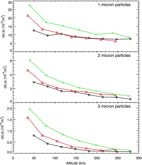
Figure 5. Profiles of particle density vs. altitude for different sized particles in the plume. The black (diamond), red (triangle), and green (cross) curves are derived from combined cubes 1, 2, and 3, respectively. The offsets between these curves are likely due to slight errors in the navigation and to errors in the pixel scale. In spite of these issues, the 3 μm particles clearly have a steeper density gradient than the 1 μm particles. Note that d(r, s) is the total number of particles in a shell of radius r per increment in size and radius.
Download figure:
Standard image High-resolution imageIn spite of these uncertainties in the amplitude of the density profiles, the three data sets show very consistent trends with height. Between 50 and 300 km above the surface of Enceladus, the 1 μm particle density declines by only a factor of 2, while the 2 μm particle density declines by about a factor of 4, and the 3 μm particle density declines by over a factor of 6. Again, the consistent trends among the different observations indicate that these data can yield useful information about the distribution and dynamics of the plume. Specifically, these data indicate that bigger particles are launched at lower velocities on average than smaller particles.
5. DERIVING THE VELOCITY DISTRIBUTION FROM DENSITY PROFILES
5.1. The Inversion Method: Onion Peeling
As discussed in Section 3.1, the density of particles at any given altitude is an integral over particles traveling with a range of speeds. However, since particles must be launched faster than a certain speed at the surface to reach a certain altitude, we can use an onion-peeling deconvolution algorithm somewhat analogous to those used to derive radial profiles of diffuse edge-on rings (see e.g., Showalter et al. 1987; de Pater et al. 1999, 2004) to derive the velocity distribution from the density profile. Starting from the top of the plume, we use the density of the plume at a given altitude to determine how many particles were launched fast enough to reach that altitude. The contribution of these particles to the rest of the profile can then be computed and removed before using the particle densities at lower altitudes to determine the number of particles that were launched at lower speeds. Because this method amounts to taking the derivative of the density profile, small errors in the density can be greatly magnified with this sort of iterative procedure. In the current situation, however, this problem is ameliorated because particles launched at a particular speed produce a density profile with a strong peak where they turn around and fall back to the surface. This means that particles detected at high altitudes do not contribute as much to the density at lower altitudes, which improves the stability to this inversion procedure.
The specific algorithm used for this analysis begins with a mean density measurement for plume particles of a given size between radii r1 and r2 from the moon's center (r2 > r1). Let us assume that the contribution from all particles with  has already been subtracted from the density measurement. Furthermore, particles must be launched with
  to reach the observed radial range. Assuming that for v2 > vo > v1 the velocity distribution function f(vo) is constant, the density of particles as a function of radius in the bin is given by (from Equation 7)
which can be evaluated to give
The average density in the bin D derived from the spectral inversions is, therefore,
where I(ro, r1, r2) is a factor that can be derived by integrating the logarithm in the above expression for d(r). Note that while a closed-form solution of this integral exists, in practice it is easy enough to evaluate numerically. We, therefore, obtain the following estimate for f(vo):
Given this value for f(vo), we can compute the contribution of these particles to the remainder of the density profile,
which can be averaged as necessary to compute and subtract the contribution of these particles to the density estimates at lower altitudes. The entire procedure can then be repeated for the next lower density measurement, etc.
The highest altitude bin is a special case for this analysis because all particles faster than a threshold speed pass through it, including escaping particles, so there is no way to determine if the particles detected here are near their maximum altitude or if they are moving well beyond the escape speed. If all particles detected in this bin are assumed to reach their highest altitude in this bin and then fall back to Enceladus, then this bin is treated just like all the others. By contrast, if all particles in this bin were launched much faster than the escape speed, then they travel with roughly constant velocity at all altitudes and contribute roughly the same density to all the measurements. To bracket the range of possibilities in the high-velocity end of the size distribution, we will here compute the velocity distributions for both these limiting cases. Intermediate cases between these limits are treated as if the topmost bin contains some fraction of particles near their maximum altitude, while the remainder are traveling well beyond the escape speed.
5.2. Results
Recall that due to its finite resolution and field of view, VIMS was only able to measure the plume signal between altitudes of 30 km and 300 km during these observations. These measurements, therefore, constrain the velocity distributions between 80 m s−1 and 180 m s−1, or between one-third and two-thirds of the escape speed. Particles launched from the surface at less than 80 m s−1 do not reach sufficient altitude for VIMS to resolve them from the bright limb, while particles launched much faster than 180 m s−1 sail beyond the edge of the field of view. This analysis, therefore, provides information about particles that fall back to Enceladus' surface.
Figure 6 shows the velocity profiles derived from the density profiles. A range of solutions are shown corresponding to different possible velocity distributions for the material in the highest altitude bin. This uncertainty in the high end of the velocity distribution does not greatly affect the 3 μm velocity profiles because the density in the highest bins is very low. By contrast, the density of 1 μm particles in the highest altitude bin is not much less than the density elsewhere in the plume, so uncertainties in the upper end of the velocity distribution lead to significant uncertainties for the remainder of the profile. Note also that the discrepancies between the density profiles from the different cubes show up again here in the velocity profiles.
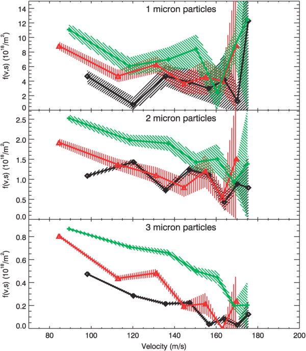
Figure 6. Velocity distributions derived from the density profiles shown in Figure 5. As before, black (diamond), red (triangle), and green (cross) correspond to data from combined cubes 1, 2, and 3, respectively. The shaded regions give the range of solutions possible depending on what fraction of the material in the highest altitude bin is falling back to Enceladus or escaping to infinity. The lines correspond to a situation in which half the material in this bin falls back to Enceladus within the bin and half escapes to infinity. Note that f(v, s) is the total flux of particles leaving the surface per increment in size and velocity.
Download figure:
Standard image High-resolution imageIn spite of these issues and uncertainties, the trends with velocity and particle size are reasonably consistent. The velocity distribution for 1 μm particles is almost a constant, while those for the 2 and 3 μm particles are progressively steeper. This confirms that larger particles are launched from the surface at lower speeds on average than smaller particles. In particular, it appears that 3 μm particles are launched from the surface with a maximum speed of only 160–180 m s−1.
6. DISCUSSION
The size distributions in Figure 4 show that the parts of the plume observed by VIMS are strongly depleted in particles with radii larger than 3 μm. Furthermore, the velocity distributions in Figure 6 indicate that only a small fraction of 3 μm particles can escape from Enceladus. This result helps explain unusually steep or narrow size distribution of the E ring that has been inferred from remote sensing (Showalter et al. 1991) and in situ (Kempf et al. 2008) observations. Apparently, only small particles seem to be accelerated sufficiently by Enceladus to reach escape velocities.
Given the assumptions and approximations used to construct the spectral models (i.e., the grains are composed of nearly pure water ice and their scattering properties can be described using Fraunhofer diffraction), as well as the uncertainties in the image pointing, the overall normalization of the density levels is quite uncertain. The most robust result of this analysis is therefore the shape of the velocity distribution, which we can parameterize using the normalized slope:
By inspection of Figure 6, we find that b(120ms−1) ∼ −0.005, − 0.010, and −0.020 s m−1 for 1, 2, and 3 μm particles, respectively. Based on the scatter among the three data sets, we estimate that the errors on these numbers are around 0.005 s m−1.
We can compare these measurements with the theoretical calculations presented by Schmidt et al. (2008) for particle acceleration in a narrow, gas-filled crack. They find that the velocity distribution of particles of size s at the surface is given by
where vg is the gas speed at the surface, which has been measured to be 300–500 m s−1 (Hansen et al. 2006; Tian et al. 2007), and sc is a critical size that depends on the gas temperature and density as well as the crack geometry.
From this expression, we can derive an expression for b:
which we can solve for the parameter sc:
Assuming vg = 400 m s−1 and the above values for b(120m s−1), we obtain sc ∼ 0.3 μm for all three particle sizes. The slopes of the velocity distributions measured by VIMS could, therefore, be consistent with the above model velocity distribution. However, if sc ∼ 0.3 μm, then f(120 m s−1) would be roughly the same for 1, 2, and 3 μm particles, while we find that there is a sharp decrease in f between 1 and 3 μm. This discrepancy could possibly be resolved by summing the flux over multiple cracks with a range of parameters.
Given the uncertainties involved in the normalization of both the spectra and the various distribution functions, we cannot at this time provide a precise measure of the total mass flux from the surface. However, integrating the relevant distributions, we can roughly estimate that the mass flux in particles larger than 0.5 μm with velocities between 80 and 160 m s−1 is between 2 and 200 kg s−1. This is much higher than the ∼0.1 kg s−1 flux of escaping particles inferred from imaging data (Porco et al. 2006), confirming that most of the mass in particles launched in the plume falls back to the surface. This particle mass flux may even be comparable to the total mass flux in gas of 120–180 kg s−1 (Hansen et al. 2006; Waite et al. 2006), which would be consistent with the Imaging Science Subsystem results that suggested comparable column masses of gas and solids at low altitudes in the plume (Porco et al. 2006).
We thank the Cassini project, the VIMS team, and the Cassini Data Analysis Program for their support of this research.
APPENDIX: PLOTS OF ALL SPECTRA
Plots of all spectra are given in Figures 7–9.

Figure 7. All the spectra from combined cube 1 used in this analysis. Data have been rebinned by a factor of 4 in wavelength for presentation. The curves show the best-fit model spectra for each data set, while the colored curves are (scaled) spectra for the same best-fit size distributions computed using Mie theory for spheres (red) and for irregular shape models 3 (green) and 5 (blue) from Pollack & Cuzzi (1980). Shaded regions are not included in the fit.
Download figure:
Standard image High-resolution image
Figure 8. All the spectra from combined cube 2 used in this analysis. Data have been rebinned by a factor of 4 in wavelength for presentation. The curves show the best-fit model spectra for each data set, while the colored curves are (scaled) spectra for the same best-fit size distributions computed using Mie theory for spheres (red) and for irregular shape models 3 (green) and 5 (blue) from Pollack & Cuzzi (1980). Shaded regions are not included in this fit. Note the bottom curve is actually the surface of Enceladus and is not used in the analysis.
Download figure:
Standard image High-resolution image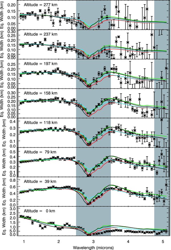
Figure 9. All the spectra from combined cube 3 used in this analysis. Data have been rebinned by a factor of 4 in wavelength for presentation. The curves show the best-fit model spectra for each data set, while the colored curves are (scaled) spectra for the same best-fit size distributions computed using Mie theory for spheres (red) and for irregular shape models 3 (green) and 5 (blue) from Pollack & Cuzzi (1980). Shaded regions are not included in this fit. Note the bottom curve is actually the surface of Enceladus and is not used in this analysis.
Download figure:
Standard image High-resolution image