


ABSTRACT
We present the observations of the contraction of the extreme-ultraviolet coronal loops overlying the flaring region during the preheating as well as the early impulsive phase of a GOES class C8.9 flare. During the relatively long, 6 minutes, preheating phase, hard X-ray (HXR) count rates at lower energies (below 25 keV) as well as soft X-ray fluxes increase gradually and the flare emission is dominated by a thermal looptop source with the temperature of 20–30 MK. After the onset of impulsive HXR bursts, the flare spectrum is composed of a thermal component of 17–20 MK, corresponding to the looptop emission, and a nonthermal component with the spectral index γ = 3.5–4.5, corresponding to a pair of conjugate footpoints. The contraction of the overlying coronal loops is associated with the converging motion of the conjugate footpoints and the downward motion of the looptop source. The expansion of the coronal loops following the contraction is associated with the enhancement in Hα emission in the flaring region, and the heating of an eruptive filament whose northern end is located close to the flaring region. The expansion eventually leads to the eruption of the whole magnetic structure and a fast coronal mass ejection. It is the first time that such a large scale contraction of the coronal loops overlying the flaring region has been documented, which is sustained for about 10 minutes at an average speed of ∼5 km s−1. Assuming that explosive chromospheric evaporation plays a significant role in compensating for the reduction of the magnetic pressure in the flaring region, we suggest that a prolonged preheating phase dominated by coronal thermal emission is a necessary condition for the observation of coronal implosion. The dense plasma accumulated in the corona during the preheating phase may effectively suppress explosive chromospheric evaporation, which explains the continuation of the observed implosion up to ∼7 minutes into the impulsive phase.
Export citation and abstract BibTeX RIS
1. INTRODUCTION
In a well received scenario, the energy release during coronal transients such as flares and coronal mass ejections (CMEs) occurs in a current sheet formed by collapsing magnetic fields of opposite polarity (Forbes 2000; Priest & Forbes 2002). The energy conversion results in the heating of local plasma and the acceleration of particles. The accelerated particles produce microwave while spiraling along magnetic fields down to the dense chromosphere, where they are stopped and emit hard X-ray (HXR) bremsstrahlung. Heated chromospheric plasma "evaporates" into closed flux tubes formed in the reconnection process, and emits soft X-rays (SXRs; see the review by Antonucci et al. 1999). This "free" energy is believed to be stored, specifically, in the strongly nonpotential, i.e., sheared or twisted, field of a filament channel which may or may not be filled with filament material (see reviews by Low 1996, 2001; Forbes 2000; Klimchuk 2001; Wu et al. 2001; Lin et al. 2003; Zhang & Low 2005). Coronal transients often result in eruptions, which are believed to be the disruption of the force balance between the upward magnetic pressure force, −∇B2/8π, of the highly sheared filament channel field, and the downward magnetic tension force, (1/4π)(B · ∇)B, of the overlying quasi-potential field.
Hudson (2000) conjectured that the energy conversion process during coronal transients would involve a magnetic implosion (referred to as the Hudson conjecture hereafter). The conjecture is based on three assumptions: (1) the transients derive their energy directly from the free energy stored in the coronal magnetic field; (2) gravitational potential energy plays no significant role; and (3) low plasma β in the corona. With the above assumptions, the conservation of energy implies that the magnetic energy decreases between the states before and after the transients. A reduction of magnetic energy, ∫VB2/8π dV, and therefore the reduction of the upward magnetic pressure, B2/8π, would inevitably result in the contraction of the overlying field so as to achieve a new force balance. Generally speaking, during the impulsive phase of a flare or the rapid acceleration phase of a CME, the energy release rate must be very high, and thus require a strong implosion. However, the large-scale motions observed in almost all flares or CMEs are explosive rather than implosive, as noted by Hudson (2000), which poses an obvious observational dilemma.
On the other hand, the contraction of flare loops themselves during the early phase of flares, which is manifested as the converging conjugate footpoints and descending looptop emission, have been reported in X-ray, extreme-ultraviolet (EUV), Hα, and microwave observations (Sui & Holman 2003; Sui et al. 2004; Liu et al. 2004, 2009; Veronig et al. 2006; Li & Gan 2005, 2006; Ji et al. 2004, 2006, 2007; Joshi et al. 2008). Sui and colleagues (Sui & Holman 2003; Sui et al. 2004) reported a downward motion of the HXR looptop source prior to the commonly observed upward expansion of the flare loop system in three homologous M-class flares that occurred between 2002 April 14 and 16. The downward motion is sustained for 2–4 minutes during the early impulsive phase of the flare with a speed between 8 and 23 km s−1 and stops at around the peak time of the HXRs. Moreover, another source above the looptop was observed while the original looptop source moved downward. This above-the-looptop source was stationary for several minutes and then moved upwards at ∼300 km s−1. In both the X3.9 flare on 2003 November 3 (Liu et al. 2004; Veronig et al. 2006) and the M7.6 flare on 2003 October 24 (Joshi et al. 2008), an apparent altitude decrease of the HXR looptop source is observed before the onset of the impulsive phase. Both flares have a gradual phase dominated by coronal thermal emission, followed by a nonthermal impulsive phase. Ji et al. (2004, 2006, 2007) reported that during the rising phase of three M-class flares, the M2.3 flare on 2002 September 9, M1.1 flare on 2004 November 1, and M6.8 flare on 2003 June 17, the EUV flare loops, Hα ribbons, HXR footpoints, and HXR looptop emission show well-correlated contraction and subsequent expansion. In both the M1.1 flare on 2004 November 1 (Ji et al. 2006) and the M6.8 flare on 2003 June 17 (Ji et al. 2007), the flare shear, indicated by Hα ribbons, HXR footpoints, and EUV flare loops, decreases steadily during both the contraction and expansion phases.
Different scenarios have been proposed to explain the above observations. Sui et al. (2004) suggested that the downward motion of the HXR looptop source is related to the change from slow to fast magnetic reconnection, which would push downward the lower bound of the current sheet that forms above the flare loops. Veronig et al. (2006) presented simulations of a collapsing magnetic trap embedded in the standard two-dimensional magnetic reconnection model, which can reproduce the altitude decrease of the HXR looptop source. However, as Ji et al. (2007) pointed out, the converging motion of the conjugate HXR footpoints cannot be accounted for in the two-dimensional models. Ji et al. (2007) therefore suggested that the contraction of flare loops is caused by the relaxation of the sheared magnetic field, a scenario consistent with the Hudson conjecture.
One may wonder how the coronal magnetic field responds to the flare loop contraction. Here we present observations of a coronal implosion showing that the EUV coronal loops overlying an eruptive filament push inward prior to the peak of the Hα emission in the flaring region. The contraction of the overlying loops is associated with the converging motion of the conjugate HXR footpoints and the downward motion of the HXR looptop source. The data sets used in our study are introduced in Section 2 and the observations are presented in Section 3. In Section 4, we discuss the implication of the observations, which sheds some light on the observational dilemma posed by the Hudson conjecture.
2. INSTRUMENTS AND DATA SET
2.1. Co-alignment
The coronal implosion event was observed between 16:00 and 17:00 UT on 2005 July 30 by the 171 Å filter (Fe ix/x, sensitive to ∼1 MK plasmas) on board the Transition Region And Coronal Explorer (TRACE; Handy et al. 1999) with a 40 s cadence, and in Hα at Mauna Loa Solar Observatory (MLSO) with a 3 minute cadence. The early phase of the GOES class C8.9 flare associated with the coronal implosion was observed by RHESSI (Lin et al. 2002). Observations from TRACE and MLSO are co-aligned with the Michelson Doppler Imager (MDI; Scherrer et al. 1995) on board the Solar and Heliospheric Observatory (SOHO; Domingo et al. 1995), after its L1 view is converted to Earth view. The pointing information of both RHESSI and SOHO is believed to be accurate. Using the routine developed by T. Metcalf (also see Metcalf et al. 2003), trace_mdi_align, in the Solar SoftWare (SSW), we cross-correlate an image obtained in the TRACE white light (WL) channel (16:14:32 UT) with an MDI continuum image (16:00:00 UT). The MLSO Hα images are aligned with MDI by manually adjusting the alignment between the facular brightening in Hα and the weak network fields in the MDI line-of-sight magnetograms. The co-alignment results are shown in Figure 1.

Figure 1. Co-alignment with SOHO MDI. Top panel, the TRACE WL image is overlaid with an MDI continuum image at 16:00:00 UT which was differentially rotated to 16:14:32 UT when the TRACE image was taken; bottom panel, the MLSO Hα image is overlaid with an MDI magnetogram at 15:59:02 UT which was differentially rotated to 16:39:32 UT when the Hα image was taken. Contour levels are 50, 200, and 800 G for positive polarities (black) of line-of-sight photospheric magnetic field, and −800, −200, and −50 G for negative polarities (gray).
Download figure:
Standard image High-resolution image2.2. RHESSI Data Analysis
RHESSI data covered the pre-impulsive phase and the major HXR burst of the C8.9 flare. HXR count rates at lower energies (below 25 keV) recorded by RHESSI as well as SXR fluxes monitored by GOES began to increase gradually as early as 16:40:00 UT, while impulsive HXR bursts (above 25 keV) are observed over 6 minutes later from 16:46:36 UT onward. The time interval from 16:40:00 to 16:46:36 UT is referred to as the preheating phase hereafter, followed by the impulsive phase from 16:46:36 UT onward. The HXR observations were discontinued at 16:49:28 UT when RHESSI went into eclipse.
We divide the time range from 16:40:00 to 16:46:36 UT into 19 consecutive 20 s intervals, excluding a 16 s interval (16:44:00–16:44:16 UT) that spanned the transition of the attenuator state from A0 to A1 at 16:44:08 UT. We then reconstruct HXR images in the 6–15 keV energy range, using the Pixon algorithm (Metcalf et al. 1996; Hurford et al. 2002). Detectors 3–8 are used as default (note that detector 7 which has a threshold of ∼10 keV is excluded for the 6–15 keV energy band), with the FWHM of the lower grid = 6 79.3 From 16:46:36 to 16:48:54 UT, for every 8 s, we reconstruct HXR sources with an integration time of 16 s in two energy bands, 6–15 keV (thermal) and 25–50 keV (nonthermal). The centroid position of each HXR source is normally determined by using a contour at 50% of the maximum brightness of each image. Due to the asymmetry of the conjugate HXR footpoints (Section 3.1), sometimes we have to use contours down to 20% level to locate the centroid position of the weaker footpoint source, or up to 80% level to accurately locate the centroid position of the stronger one.
Spatially integrated flux spectra are obtained using the standard RHESSI software and analyzed with the Object Spectral Executive (OSPEX) package, for nine consecutive 40 s intervals from 16:40:00 to 16:46:16 UT excluding the same 16 s interval that spanned the transition of the attenuator state, and for eight consecutive 20 s intervals from 16:46:16 to 16:48:56 UT. In the spectral study, we use all detectors except detectors 2 and 7 to obtain the spectra. We use 1 keV wide energy bins from 3 to 40 keV, 3 keV bins up to 100 keV, 5 keV bins up to 150 keV, and 10 keV bins to 250 keV. Note that the thin attenuator set in (A1 state) at 16:44:08 UT, so all the spectra are fit only for the energies above 10 keV, as our knowledge of the attenuator transmission below 10 keV is in question at the 20%–30% level (R. Schwartz 2008, private communication).
3. OBSERVATIONS AND ANALYSIS
3.1. Overview of the Observations
The eruption occurred in the NOAA active region 10792. Major features of the event are displayed in Figure 2, which shows TRACE 171 Å observations and the corresponding running difference images. About 1 hr prior to the eruption, a collection of coronal loops (labeled "L"), which are apparently twisted or braided, gradually appeared from approximately 16:00 UT and became fully visible at 16:09:01 UT (Figures 2(a) and (d)). Some of the loops appeared to have a very flat looptop, indicating that the magnetic field they trace are probably highly stressed. However, we must be cautious in interpreting these observations due to possible projection effects. Moreover, a narrow filter like TRACE 171 Å only shows plasmas in a narrow temperature range. Note located to the west of the loops of interest, the "potential-like" loops are a remnant of the postflare arcade due to a major flare (X1.3) occurring about 10 hr ago (2005 July 30, 06:30 UT) in the center of the same active region. They may not play a significant role in the eruption studied in this paper since they apparently survive the eruption (Figure 2(i)).

Figure 2. TRACE 171 Å images and the corresponding running difference images. All TRACE images are registered with the image taken at 16:00:30 UT and corrected for solar rotation. In Panel (a), a slit is placed across a group of coronal loops, which became fully visible in TRACE 171 Å at 16:09:01 UT (labeled "L" in Panel (d)). Panels (b) and (c) are overlaid with HXR contours at 30% and 60% of the maximum brightness of each individual RHESSI image in the 6–15 keV (white) and 25–50 keV (black) energy range. Black arrows mark a representative contracting loop; and white arrows indicate the filament in emission (see the text).(An mpeg animation of this figure is available in the online journal.)
Download figure:
Standard image High-resolution imageIn Figures 2(b) and (c), the TRACE images are overlaid with RHESSI HXR contours. The detailed evolution of the HXR emission is shown in Figure 3. During the preheating phase from 16:40:00 to 16:46:36 UT, the flare emission was dominated by thermal emission in the 6–15 keV energy range (see also Section 3.3). From 16:40:40 to 16:44:00 UT, the flare emission took the form of a loop, whose endpoints were roughly co-spatial with the conjugate HXR footpoints during the impulsive phase. From 16:44:16 UT onward, the thermal emission changed into a compact looptop source. After the onset of the impulsive HXR burst at 16:46:36 UT, the flare exhibited two distinct footpoints in the 25–50 keV energy range, with the southern footpoint appearing first, as well as the compact looptop source in the 6–15 keV energy range.

Figure 3. Evolution of HXR emission. The figure shows a series of RHESSI images in the 6–15 keV energy range, overlaid by contours at 20%, 50%, and 80% of the maximum brightness, Imax (photons cm−2 s−1 arcsec−2) of each RHESSI image obtained for the same time interval in the 25–50 keV energy range. Imax is shown in each image, also shown is Ctot, the total counts accumulated by the detectors used for image reconstruction, with gray (black) colors indicating the 6–15 keV (25–50 keV) energy band.
Download figure:
Standard image High-resolution imageThe loop half-length of the flare loop mapped out by the HXR sources measures about 109 cm, while it is as large as 5 × 109 cm for the group of crisscross coronal loops (Figure 2). The coronal loops began to contract starting around 16:42 UT until 16:54 UT. The contraction is apparent in the running difference images (Figures 2(f) and (j)), in which the loops brightened at the inner side and darkened at the outer side. A representative contracting loop is indicated by a black arrow in Figure 2(f). One can see that the brightening and darkening pattern reversed as the loop began to expand later (indicated by the black arrow in Figure 2(k)). With the expansion of the coronal loops, a filament located underneath was observed to become partially in emission (indicated by white arrows in Figures 2(h) and (k); see also Section 3.4), and the whole structure, both the expanding coronal loops and the heated filament, were observed to erupt in TRACE 171 Å at about 17:02 UT (Figures 2(i) and (l)). The expansion of the stressed loops of interest, and the consequent eruption, occur during the gradual phase of the flare. It may be associated with the occurrence of the "torus instability" (Kliem & Török 2006), which is often induced in response to the lateral expansion of a toroidal flux rope.
To summarize, the major sequence of the event studied in this paper is as follows.
- 1.16:09:01 UT, stressed overlying coronal loops become fully visible in EUV.
- 2.16:40:00 UT, GOES SXR flux and RHESSI HXR count rates at lower energies (below 25 keV) started to increase.
- 3.16:40:00–16:46:36 UT, the flare emission was dominated by a thermal looptop source in the 6–15 keV energy range, with the temperature of 20–30 MK (Section 3.4).
- 4.16:42 UT, the coronal loops began to slowly contract.
- 5.16:46:36–16:48:24 UT, the major HXR burst of the flare was observed. A pair of conjugate footpoint sources appeared besides the looptop emission.
- 6.16:50 UT, the contracting coronal loops located at higher altitudes began to expand, and the originally dark filament located underneath was observed to be partially in emission.
- 7.16:54 UT, the contracting coronal loops located at lower altitudes began to expand.
- 8.17:02 UT, the expanding coronal loops and the heated filament were observed to erupt together.
- 9.17:24 UT, a fast CME (∼1000 km s−1) was observed in SOHO LASCO C2, with a central position angle (measured from the north pole counterclockwise) of 74°, and an angular width of 84°.
- 10.18:20 UT, postflare arcade associated with the eruption was observed in TRACE 171 Å (see the animation accompanying Figure 2).
The coronal implosion, which is manifested as the contraction of the overlying coronal loops as well as the contraction of the underlying flare loop, is studied in detail in Section 3.2. The two other interesting aspects of this event, namely, the spectral evolution of the flare, and the heating and the consequent eruption of the filament, are investigated in Sections 3.3 and 3.4, respectively.
3.2. Coronal Implosion
A horizontal slit of 186 pixels long (93'' in the east–west direction) and 20 pixels wide (10'' in the north–south direction) is placed across the group of contracting coronal loops (Figure 2(a)), and the slices of TRACE images cut by the slit are rotated to a vertical direction and placed on the time axis in Figure 4(a). The slice width on the time axis reflects the exposure duration of each image, which is about 32.77 s throughout most of the data set, and voids are due to data gaps. From Figure 4(a) one can see that the collection of coronal loops of interest is mainly composed of three clusters of loops at different altitudes. All three clusters of loops contracted at approximately the same speed (4–7 km s−1), starting at approximately the same time (∼16:42 UT). The higher and middle clusters of loops appear to expand first (∼16:48 UT) while the lower cluster of loops were still contracting till about 16:53 UT, and then began to expand. The average speed of expansion estimated from four slices of images during the time period 16:53:58–16:56:01 UT is about 60 km s−1 (Figure 4(a)). The expansion speed of the higher and middle clusters of loops is hard to measure because they become very diffuse while expanding (also see the animation accompanying Figure 2). Normalized Hα emission (Figure 4(d)), which is obtained by integrating over the whole flaring region (defined in Section 3.4), shows minimal increase during the preheating phase, but significant enhancement after the onset of the impulsive phase. Hα emission has been reported to peak preferentially simultaneously with SXR (e.g., Veronig et al. 2002), so it is also an indicator of the heating of the chromosphere, primarily due to precipitating particle beams. The expansion of the coronal loops from about 16:50 UT onward roughly coincided with the sharp increase of the Hα emission which peaked between 16:48:31 and 16:54:33 UT as determined from the Hα images with 3 minutes cadence. By the time the expanding coronal loops were observed to erupt in TRACE 171 Å (17:02 UT), the Hα emission had declined to the pre-impulsive phase level. Also plotted in Figure 4(e) are RHESSI count rates at 1 s resolution in the 6–15 keV (gray) and 25–50 keV (black) energy range, and GOES 1–8 Å (dotted line) and 0.5–4 Å (dashed line) SXR fluxes. In Figure 4( f ), we plot the time derivatives of GOES fluxes which peaked approximately at the same time as the HXR burst at about 16:47:30 UT, which is known as the Neupert effect (Neupert 1968).
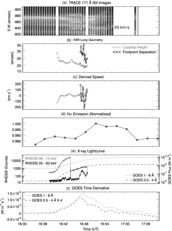
Figure 4. Coronal implosion observed in EUV and X-rays. (a) Slices of TRACE 171 Å images cut by the horizontal slit as defined in Figure 2(a) are rotated to a vertical direction and placed on the time axis, with the slice width reflecting the exposure duration of each image. (b) Time evolution of the height of the HXR looptop emission (in a "+" symbol) as well as the separation between two conjugate HXR footpoints (in a "×" symbol). (c) Derived speed from (b), using numerical differentiation. (d) Normalized Hα emission which is integrated over the flaring region. (e) RHESSI count rates (s−1) in the 6–15 keV (gray) and 25–50 keV (black) energy range (scaled by the y-axis on the left), and GOES 1–8 Å (0.5–4 Å) SXR fluxes in dotted (dashed) line (scaled by the y-axis on the right). Note that the sudden transition in the 6–15 keV light curve was due to the change of the attenuator state from A0 to A1 at 16:44:08 UT, and that the RHESSI observation was discontinued at 16:49:28 UT when RHESSI went into eclipse. (f) Time derivatives of GOES 1–8 Å (0.5–4 Å) fluxes in dotted (dashed) line, which serve as a complement to the RHESSI observation.
Download figure:
Standard image High-resolution imageThe contraction of the overlying coronal loops is associated with the converging motion of the conjugate HXR footpoints as well as the downward motion of the HXR looptop source. In Figure 5, the centroid positions of HXR sources4 (the looptop source is denoted by a "+" symbol and the footpoint source by a "×" symbol) are projected onto background images in different wavelengths, and their time evolution is color-coded. All the centroid positions and images are differentially rotated to 16:40:34 UT, when the TRACE 171 Å image (top left panel in Figure 5) was taken. One can see that the conjugate footpoints were generally approaching each other during the impulsive phase, while the looptop source exhibited a descending motion toward the solar surface as early as the preheating phase. The TRACE 171 Å image shows that the contracting coronal loops (labeled "L") were overlying an elongated absorption feature (labeled "F"), which corresponds to the dark filament observed in Hα, whose northern end is located close to the flaring region (bottom left panel in Figure 5). The eruption is presumably due to the interactions of the magnetic fields from two pairs of sunspots, which are labeled "P1," "N1," and "P2," "N2," respectively, in the TRACE white-light image (bottom right panel in Figure 5), with "P" ("N") indicating positive (negative) polarities. The polarities are determined from the corresponding MDI line-of-sight magnetogram (top right panel in Figure 5), which is overlaid with the calculated neutral lines. One can see that the southern footpoint is confined to the penumbrae of the major sunspot, P1, while the northern footpoint is confined to the penumbrae of the sunspot, N2. It is interesting that both HXR footpoints were approaching the umbrae of P1.

Figure 5. Time evolution of centroid positions of the HXR looptop emission (in a "+" symbol) and of the HXR footpoints (in a "×" symbol). The centroid positions at different times (color-coded, indicated by the color bar) are projected onto a TRACE 171 Å image (top left), an MDI magnetogram (top right), an MLSO Hα image (bottom left), and a TRACE white-light image (bottom right), respectively. All the centroid positions and images are differentially rotated to 16:40:34 UT, the time when the TRACE 171 Å image was taken. The eruptive filament (see the text) is labeled "F" in the TRACE 171 Å image and the corresponding Hα image. The bunch of contracting coronal loops (see the text) is labeled "L" in the TRACE 171 Å image. The MDI magnetogram is overlaid with contours indicating the neutral line of the line-of-sight magnetic field. The two pairs of the sunspots that involved in the flare (see the text) are labeled "P1," "N1," and "P2," "N2," respectively, in the TRACE white-light image, with "P" ("N") indicating positive (negative) polarities.
Download figure:
Standard image High-resolution imageThe separation of the conjugate HXR footpoints is defined as the distance between their centroid positions ("×" symbol; Figure 4(b)). The converging/separating speed can be derived from numerical differentiation of the distance–time profile after it is smoothed with a 3 point boxcar (Figure 4(c)). The "height" of the looptop HXR source is defined as the perpendicular distance of its centroid position to the line connecting the centroid positions of the distinct conjugate footpoints observed at 16:47:08 UT (Figure 3). Similarly, the speed of downward/upward motions is also derived from numerical differentiation. The height–time profile of the looptop shows a two-stage evolution, rapid descent from 16:40:00 to 16:42:40 UT, followed by slow, quasi-static descent from 16:42:40 to 16:49:00 UT. The relative motion of the conjugate footpoints shows an oscillatory converging trend during the impulsive phase.
To verify if HXR source motions in Figure 6 are real, we use longer integration time and wider energy band for better count statistics. Using the Pixon algorithm, we reconstruct HXR sources with an integration time of 24 s in two energy bands, 6–15 keV (using detectors 3–6 and 8) and 20–60 keV (using all detectors), for every 4 s from 16:46:36 to 16:49:04 UT. Similarly, we use the CLEAN algorithm (Hurford et al. 2002) to reconstruct all the HXR sources (the only difference is that we use detectors 3–8 for the 20–60 keV energy band). In the same way as described above, we determine the separation between conjugate footpoints and the height of the looptop source with respect to the distinct conjugate footpoints observed at earliest time, using the centroid positions as well as the peak brightness positions of HXR sources, indicated in dark and gray colors in Figure 7, respectively. Both the altitude decreasing motion of the looptop and the oscillatory converging motion of the footpoints persist.
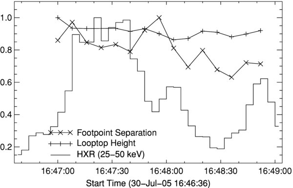
Figure 6. Normalized looptop height, and conjugate footpoint separation with respect to time, in comparison to the HXR light curve in the 25–50 keV energy band at a 4 s resolution.
Download figure:
Standard image High-resolution image
Figure 7. Normalized looptop height, and conjugate footpoint separation with respect to time, in comparison to the HXR light curve in the 20–60 keV energy band at 4 s resolution. Distances measured using the centroid position (peak brightness position) of HXR sources are in dark (gray) colors. Top (bottom): HXR sources are reconstructed using the Pixon (CLEAN) algorithm.
Download figure:
Standard image High-resolution image3.3. Spectral Evolution of the Flare
To estimate the relative contributions of the thermal and nonthermal components of the HXR emission, we fit the spatially integrated, background subtracted spectra with an optically thin thermal bremsstrahlung function plus a broken power-law function. The spectral index below the break energy is fixed at γ = 2 to approximate a constant electron flux below a lower cutoff energy. The spectral index above the break energy and the break energy itself are both free parameters in the spectral fitting.
Figures 8 and 10 show the spectral evolution of the flare. During the preheating phase (16:40:00–16:46:36 UT), the spectra are fit with a thermal component with a temperature of 20–30 MK (Figures 8(a) and (b)), corresponding to the thermal looptop emission observed in the 6–15 keV energy range (Figure 3), and a steep nonthermal component with a spectral index γ ≈ 6. The spectra during the impulsive phase exhibit a significant nonthermal component with the spectral index γ = 3.5–4.5, in addition to the isothermal component with a temperature of 17–20 MK (Figure 8(c)). The nonthermal component is corresponding to the conjugate footpoint sources observed above 25 keV (Figure 3), which is generally believed to be produced by thick-target bremsstrahlung in or near the chromosphere.

Figure 8. Typical RHESSI spatially integrated, background-subtracted spectra and the corresponding spectral fits during the preheating phase (a–b) and the impulsive phase (c). The thermal component is in a dotted line, and the nonthermal component in a dashed line. The energy range for spectral fits is 10–50 keV. The attenuator state (A0 or A1) is indicated in the title of each panel.
Download figure:
Standard image High-resolution imageSpatially resolved spectra of the looptop and footpoint sources during the time interval of the major HXR burst at about 16:47 UT are obtained in a imaging spectroscopy analysis (Figure 9). The spectra of both footpoints can be fit with a single power-law function, whose indices are approximately equal to that of the nonthermal component in the spatially integrated spectra. One can also see that the spectrum of the looptop source is very similar to the spatially integrated spectra during the preheating phase, indicating that the preheating phase was indeed dominated by the coronal emission.
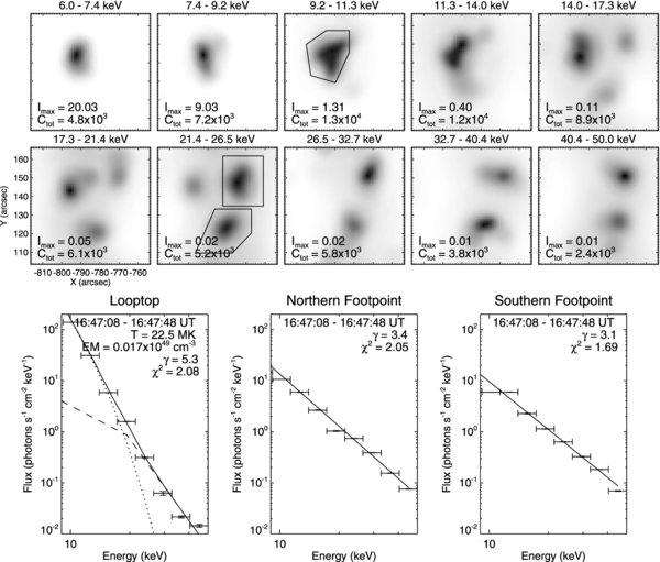
Figure 9. Imaging spectroscopy for a 40 s interval covering the major HXR burst at about 16:47 UT on 2005 July 30. Shown in the top panel are Pixon images made with detectors 3–8 in 10 logarithmically spaced energy bins from 6 to 50 keV. Indicated in the lower left corner of each image are the maximum brightness, Imax (photons cm−2 s−1 arcsec−2), of each individual Pixon map, and the total counts accumulated by the detectors used, Ctotal. The three hand-drawn polygons are used to obtain the spectra of the looptop and the conjugate footpoint sources in the bottom panel. The looptop spectrum is fit with a isothermal function plus a broken power-law function with the spectral index below the break energy being fixed at 2. The spectra of both footpoints are fit with a single power-law function.
Download figure:
Standard image High-resolution imageThe density of the looptop source (Figure 10(b)) is inferred by using the formula,  , where EM is the emission measure obtained in the thermal fits, S is the area inside the 50% brightness contour of the looptop source at 6–15 keV (∼400 arcsec2), reconstructed with the CLEAN algorithm in the corresponding time intervals, and f is the volume filling factor. f is in the range of 0.03–0.08, constrained by fractal dimensions measured in solar flares (Aschwanden et al. 2008). Here f is assumed to be 0.1 to approximate a lower limit of the density. We can then infer the pressure, P = nkBT, of the plasma in thermal emission (Figure 10(d)), where kB is Boltzmann's constant. One can see that the emission measure as well as the derived density and pressure increased steadily during the preheating phase, but exhibit an oscillatory feature during the impulsive phase, apparently modulated by the impulsive HXR bursts (e.g., Battaglia et al. 2005).

Figure 10. Spectral fitting results and derived physical variables with respect to time. (a) The temperature, T (MK) (scaled by the y-axis on the left) and the spectral indices, γ (scaled by the y-axis on the right). Overplotted are the isothermal temperature derived from two GOES bands (solid line) and that corrected for a systematic bias with respect to RHESSI data (see the text). (b) The emission measure, EM (1049 cm−3). The corresponding GOES result is also plotted. (c) The density of the looptop source, n (109 cm−3), derived from the formula,  , by measuring the area of the looptop source, S, in the corresponding RHESSI image, and assuming the filling factor f = 0.1. (d) The thermal pressure of the looptop source (P) derived from the formula P = nkBT (dyne cm−2). (e) RHESSI light curves in three energy bands are shown here to provide context for spectral evolution. The horizontal error bar indicates the integration time to obtain the spectra.
Download figure:
Standard image High-resolution imageFrom the flux ratio in the two GOES wavelengths bands, i.e., 0.5–4 Å and 1–8 Å, one can also calculate an isothermal temperature, TGOES (solid line in Figure 10(a)). Battaglia et al. (2005) found a systematic bias in peak flare temperatures determined with RHESSI and GOES data, i.e., TRHESSI = 1.31TGOES + 1.47 (dotted line in Figure 10(a)). The reason is that GOES measurements are dominated by photons at lower energies, compared to RHESSI. Even with the above correction, TRHESSI is still significantly higher than TGOES during the early preheating phase (Figure 10(a)). The two temperatures, however, approximately agree with each other as time progressed, which suggests that flare plasma was highly multithermal during the early preheating phase, but tended to be isothermal in the later evolution. Battaglia et al. (2005) also found that the emission measure derived from the GOES data is generally larger than that from the RHESSI data (EMRHESSI = 0.1EMGOES on the average). In our case, during the impulsive phase, the GOES emission measure serves as a higher bound for that derived from the RHESSI spectral fitting (Figure 10(b)); during the preheating phase, however, the emission measure from GOES data is significantly larger than that from RHESSI data, which is consistent with the existence of a superhot component (20–30 MK) in comparison to the main component of flare plasma (10–20 MK).
3.4. Heating and Eruption of the Filament
An elongated brightening was observed in TRACE 171 Å at about 16:55 UT (Figures 2(h) and (k); indicated by a white arrow), which is due to the heating of a filament. By comparing TRACE 171 Å images and MLSO Hα images at approximately the same time, one can see that the dark filament observed in Hα at about 16:45 UT (indicated by an arrow; Figure 11(d)) is co-spatial with a dark, elongated absorption feature observed in TRACE 171 Å (Figure 11(a); see Figure 5(a)). At about 16:54 UT, the southern part of the filament in EUV became in emission (indicated by an arrow in Figure 11(b)). In the corresponding MLSO Hα image (Figure 11(e)), the bulk of the filament disappeared, only its northern end was still visible in absorption, marked by an arrow. At about 17:02 UT, the filament is observed to erupt in TRACE 171 Å (Figures 11(e) and 2(l)), while in the corresponding Hα image (Figure 11( f )), the filament disappeared completely. However, the eruption does not result in a complete loss of the filament, i.e., it is a partial eruption (Gilbert et al. 2007), as the absorption feature became visible in TRACE 171 Å in the aftermath of the eruption as early as about 17:20 UT, and part of the filament re-appeared in Hα about 1 hr later.
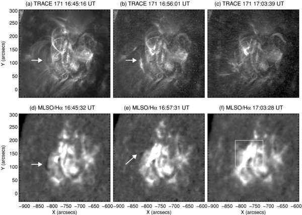
Figure 11. Partial filament eruption observed in TRACE 171 Å and the corresponding MLSO Hα images. The rectangle in Panel (f) defines the region over which Hα emission is integrated and shown in Figure 4(d).
Download figure:
Standard image High-resolution imageMouradian et al. (1995) classified disparition brusques (DBs), the sudden disappearance of filaments/prominences in Hα observations, into two categories, dynamic and thermal DB. Dynamic DBs in their definition show acceleration and complete disappearance, followed by a reappearance on a timescale of days; on the other hand, thermal DBs exhibit little, if any, upward motion but show significant filament disappearance (which they attributed to heating and subsequent ionization of filament plasma), followed by reappearance of the filament within hours. They claimed that dynamic DBs are associated with CMEs, whereas thermal DBs are only local disturbances of the lower corona. The Hα observation in our study conforms to the definition of thermal DB, but the filament is observed to be first heated, then partially erupt in EUV, and result in a fast CME in white light, first observed in SOHO LASCO C2 at 17:24:19 UT with an average speed of above 1000 km s−1, according to the LASCO CME Catalog.5 This suggests that to classify DB into dynamic and thermal DB may be misleading. Whether a filament eruption results in a CME and how long it takes for the filament to reappear most likely depends on the nature of the eruption, i.e., whether it is a full, partial or failed eruption (Gilbert et al. 2007).
4. DISCUSSION AND CONCLUSION
The contraction of the overlying coronal loops during the early phase of the flare in our observations (Figure 4) is, in our opinion, a manifestation of the release of the free magnetic energy and the consequent decrease of the magnetic pressure in the flaring region, dubbed "coronal implosion" by Hudson (2000). The contraction is associated with the downward motion of the HXR looptop source and the converging motion of the conjugate HXR footpoints, which have been interpreted by some authors as the relaxation of the sheared magnetic field (e.g., Ji et al. 2007; Liu et al. 2009). The expansion of the coronal loops following the contraction is associated with the significant enhancement in Hα emission in the flaring region, indicating the heating of the chromosphere, due primarily to precipitating particle beams. It is the first time that such a large scale contraction of the coronal loops that overlie a flaring region has been observed. The coronal loops are essentially composed of three clusters of loops (Section 2.4). The contraction of the lower cluster is sustained for about 12 minutes at an average speed of −7 km s−1, and for the higher and middle clusters, it is sustained for about 6 minutes at an average speed of −4 and −6 km s−1, respectively.
4.1. Why is Coronal Implosion so Rare?
The fact that the coronal implosion is so rarely observed may have something to do with the assumptions on which the Hudson conjecture is based. Although the three assumptions (see Section 1) are generally true in the corona, the third assumption, β ≪ 1, may be violated in the magnetic reconnection region, where the breakdown of the ideal MHD approximation is inherently required; and in the associated flaring region, where the thermal pressure may not be ignored. By definition,
In the typical hot corona condition (ne ≈ 109 cm−3 and T ≈ 3 × 10⁶ K, B = 10 G), plasma β is ∼0.2 (Aschwanden 2006, p. 28, Section 1.8). At the looptop of the flaring loop in our observation (ne ≈ 50 × 109 cm−3, T ≈ 20 MK), the plasma β is as large as 0.7, assuming that the ionization fraction is of order unity and that the magnetic field B ≈ 100 G. This suggests that plasma diffusion across field lines may not be ignored at the dense, hot flare looptop.
Thus, when a flare has not caused any significant changes of the confining field, the decrease of the magnetic pressure can, in principle, be compensated by the increase of the thermal pressure in the flaring region, partly due to the localized heating of coronal plasmas, and partly due to two types of chromospheric evaporation (Fisher et al. 1985), namely, "gentle" evaporation driven by low electron fluxes (e.g., Milligan et al. 2006), or by thermal conduction (e.g., Zarro & Lemen 1988), and "explosive" evaporation driven by high nonthermal electron fluxes (e.g., Brosius & Phillips 2004). Explosive chromospheric evaporation overwhelms the other two mechanisms during the main impulsive phase of the flare. Hydrodynamic simulations of this particle-driven chromospheric heating process yield upflowing plasma with peak electron densities of about 1011 cm−3 and peak temperatures of (1.5–2) × 107 K (e.g., Mariska et al. 1989). Simulations of the evaporation process driven by thermal conduction show minimal effects on the magnetic reconnection, because the evaporated plasma fills mainly the lower part of the flare loops (Yokoyama & Shibata 2001), but for more energetic explosive evaporation, the chromospheric material may only be partially confined in closed magnetic flux tubes, thereby impacting the pressure balance in the higher coronal region. This may find support in some SXR spectroscopy analyses in the Solar Maximum Mission (SMM) era, which suggest that the total amount of hot upflowing plasma during the flare rise time exceeds the amount of stationary plasma contained in the loop close to the flare peak time (e.g., Karpen et al. 1986; Doschek et al. 1989). Moreover, as new field lines reconnect progressively above the reconnected loops, the chromospheric evaporation also extends into the corona. Hence, chromospheric evaporation, especially the explosive one, may play a significant role in the pressure balance of the flaring region.
On the other hand, if the overlying field lines that provide the confinement undergo a breakout reconnection (Antiochos et al. 1999), or, are stretched and thereby reconnected below a rising and expanding fluxrope (Forbes 2000), the reduction of the magnetic tension may be comparable to or greater than the reduction of the magnetic pressure in the flaring region, so that implosion is no longer a concern.
4.2. What is the Role of Preheating?
Recent progress in the study of magnetic reconnection (e.g., Cassak et al. 2005, 2006, and references therein) shows that slow, collisional reconnection can dominate the dynamics of a system for a long time. When the dissipation region becomes thinner and the resistivity drops below a critical value, fast, collisionless reconnection sets in abruptly, increasing the reconnection rate by many orders of magnitude and resulting in a magnetic explosion, a picture similar to the catastrophe model of solar flares (Lin & Forbes 2000). In our case, the thermal preheating phase may correspond to the slow reconnection stage, during which the released free energy heats local plasmas and drives gentle chromospheric evaporation; fast reconnection sets in at the onset of the impulsive phase, which considerably increases the fraction of high-energy electrons, as indicated by a reduction of spectral index from 6 to 4 (Figure 10(a)). The harder electron beam can presumably drive explosive chromospheric evaporation.
The preheating phase, characterized by strong SXR emission or HXR thermal emission at lower energies within several minutes prior to the impulsive HXR bursts (e.g., Machado et al. 1986; Veronig et al. 2002), suggests that the coronal atmosphere is already heated to a dense and hot state prior to impulsive electron acceleration. Emslie et al. (1992) argued that if the preflare atmosphere is dense, then the column depth of the corona is enhanced and the stopping distance for the electrons is shorter. Thus, the bulk of the accelerated electrons lose their energy in the corona, and the chromospheric evaporation will be strongly suppressed, due not only to reduced energy deposited in the chromosphere, but also to the increased inertia of the overlying material. In the two successive flares studied by Strong et al. (1984), the first flare exhibited the usual line broadening and blueshifts, but the second did not show any significant mass motions. This was interpreted as the lack of evaporation in the second flare, because the flare loop had been filled with material from the previous flare. In our case, the flare loop density gradually increased with time to ∼4 × 1010 cm−3 prior to the impulsive phase. This may explain why the implosion of overlying coronal loops continued up to 7 minutes into the impulsive phase (Figures 4(a) and (b)), and significant enhancement in Hα emission in the flaring region lagged behind the major HXR burst (Figure 4(d)). This dense plasma accumulated in the corona during the preheating phase seems to be consistent with the universal presence of a strong stationary component in flare SXR line profiles (e.g., McClements & Alexander 1989).
The increase in the flare loop density during the preheating phase could be due to the "gentle" chromospheric evaporation in response to the hot coronal source (20–30 MK). The thermal flux conducted into the cool layers of atmosphere, F = κT5/2∇T, is 3.6 × 10¹⁰–1.5 × 10¹¹ erg cm−2 s−1, if we estimate the flux by 10−6T7/2/L, where L is the half-length of the flare loop mapped out by the HXR sources (≈109 cm) and κ is the classical Spitzer coefficient (10−6 erg cm−2 s−1 K−7/2). Such intensive conductive heating implies a major dynamic rearrangement in the transition region and the upper chromosphere. If the conduction flux is balanced by the enthalpy flux of the evaporation flow (Antiochos & Sturrock 1978), i.e.,

where  is the sound speed of the evaporation flow, then the density of the evaporating flare loop
(Shibata & Yokoyama 2002). Inserting in Equation (3) T = 20 MK and L = 109 cm, we get the density prior to the impulsive phase, n = 4 × 1010 cm−3, which is in agreement with the values derived from spectral fitting (Figure 10). The flare loop density determined by Equation (3) is supposed to be a lower limit, as it does not take into account the accumulation of the evaporated plasma in the flare loop (Shibata & Yokoyama 2002). The fact that the two numbers agree with each, however, is not surprising, as radiative losses are not accounted for in Equation (2).
Flares that exhibit a preheating phase dominated by coronal thermal emission have only been reported in four events in the literature (MacNeice et al. 1985; Uchida et al. 2001; Veronig et al. 2006; Joshi et al. 2008). MacNeice et al. (1985) found in an M1.4 flare on 1980 November 12 that the emission in the Fe xxv line (20 MK) was enhanced at the flare looptop, and that the Ca xix resonance line was broadened during the preheating phase. They also reported and that blueshifts corresponding to explosive chromospheric evaporation are seen in Ca xix after the onset of the impulsive phase. Uchida et al. (2001) reported in an M1.5 flare on 1993 April 22 a thermal source of 80 MK during the preheating phase, located between the conjugate footpoints that appear in the impulsive phase. Recently, the downward motion of the looptop source was observed by RHESSI during the preheating as well as the early impulsive phase in an X3.9 flare on 2003 November 3 (Veronig et al. 2006), and in an M7.6 flare on 2003 October 24 (Joshi et al. 2008). Of all four events, the M7.6 flare on 2003 October 24 is the only one that has TRACE data coverage. We note that the coronal loops overlying the flaring region observed in TRACE 195 Å display obvious contracting motions starting even prior to the preheating phase. We use two slits (defined in Figure 12) to measure the large-scale motions of both the coronal loops and the 195 Å looptop emission. The contracting speed of the overlying coronal loops in both slits is about 5 km s−1 (Figure 13(a); not necessarily the same loops as we use different slits), and the speeds of the looptop's descending, as well as ascending, motions are comparable to the measurements by Joshi et al. (2008, their Figure 6). The overlying coronal loops in Slit 2 show signs of expansion during the impulsive phase, with an approximate speed of 10 km s−1, but the loops later become too diffuse (after ∼02:50 UT) to allow the accurate measurement of the speed.

Figure 12. Two slits that we used to measure the contracting speeds of the overlying coronal loops and the flare looptop emission in the 2003 October 24 event. Panel (a) shows the slit that cuts through the contracting coronal loop from 01:36:52 to 02:29:25 UT; Panel (b) shows the slit that cuts through the contracting flare looptop source from 02:29:01 to 03:08:59 UT.
Download figure:
Standard image High-resolution image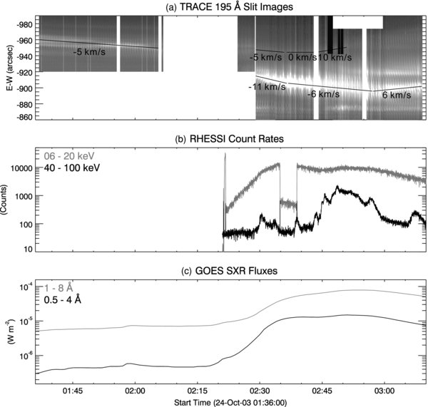
Figure 13. Coronal implosion observed in TRACE 195 Å in the 2003 October 24 event. (a) Slices of TRACE 195 Å images cut by the horizontal slits as defined in Figure 12 are rotated to a vertical direction and placed on the time axis. (b) RHESSI count rates (in 1 s resolution) in the thermal (6–20 keV; gray) and nonthermal (25–50 keV; black) energy ranges. Note that the sudden transitions in the RHESSI light curves were due to the change of the attenuator states. (c) GOES 1–8 Å (0.5–4 Å) SXR fluxes (W m−2) in gray (black) line.
Download figure:
Standard image High-resolution image
4.3. Concluding Remarks
We propose that during the preheating phase (slow reconnection stage) the increase of the thermal pressure is mainly due to localized heating and gentle evaporation, which is not enough to compensate for the decrease of the magnetic pressure, because the released free energy can escape in other forms, such as optically thin radiation, thermal conduction, and hydromagnetic waves. Thus, the magnetic structure surrounding the flaring region, observed as the EUV coronal loops, pushes inward. After the onset of the fast reconnection (impulsive phase), however, the bulk of particles are accelerated to much higher energies and can no longer be stopped in the corona as in the preheating phase. Thick-target bremsstrahlung is thereby strongly enhanced, which drives explosive chromospheric evaporation. This results in the expansion of the magnetic structure surrounding the flaring region, and probably the heating of the filament whose northern end is located close to the flare region, which eventually leads to the eruption of the whole structure and the consequent CME. For the overlying loops to "know" the reduction of the magnetic pressure in the reconnection region, however, the preheating phase should last for at least
where L is the height of the overlying loops with respect to the reconnection location and VA is the Alfvén speed in the corona. We, therefore, suggest that a prolonged preheating phase dominated by coronal thermal emission is a necessary condition for the observation of coronal implosion. The dense plasma accumulated in the corona during the preheating phase may effectively suppress explosive chromospheric evaporation, which explains the extending of the observed implosion up to ∼7 minutes into the impulsive phase. An interesting question arises whether a similar process could occur in flare-like events, such as "active region transient brightenings," so implosion on a smaller scale might be observed in the nonflaring region. High-resolution spectroscopy as well as numerical experiment is needed to test this scenario in the future work.
The authors acknowledge the TRACE and RHESSI consortia for the excellent data. R.L. thanks Jun Lin for helpful discussion. R.L. and H.W. were supported by NASA grant 8AJ23G and 8AQ90G, and by NSF grant ATM-0548952.
Footnotes
- 3
The Pixon algorithm itself can decide which detectors to keep and which to discard. But to include more detectors will result in higher computational expense. Detector 9 is excluded because its FWHM (183
2) is greater than the size of the maps we are making (128'' × 128''). Detectors 1 and 2 have the finest angular resolutions, but generally do not add much information to the Pixon map. Like detector 7, detector 2 is also excluded for lower energies because of its higher energy threshold. Moreover, detectors 2 and 7 have significantly worse energy resolution (3 keV FWHM and 7–10 keV FWHM, respectively) than the others. - 4
The centroid as well as the peak brightness locations are obtained using the Image Flux tool in the standard RHESSI software. However, the uncertainty on the location is not well defined. It depends on the details of the image, the photon statistics, and on the systematic as well (B. Dennis 2008, private communication). In general, the accuracy is better than the resolution of the finest grid that is used to make the image, given good enough photon statistics and fine enough pixels.
- 5