


ABSTRACT
We present high-resolution Hubble Space Telescope images of all 35 active galactic nuclei (AGNs) with optical reverberation-mapping results, which we have modeled to create a nucleus-free image of each AGN host galaxy. From the nucleus-free images, we determine the host-galaxy contribution to ground-based spectroscopic luminosity measurements at 5100 Å. After correcting the luminosities of the AGNs for the contribution from starlight, we re-examine the Hβ RBLR–L relationship. Our best fit for the relationship gives a power-law slope of 0.52 with a range of 0.45–0.59 allowed by the uncertainties. This is consistent with our previous findings, and thus still consistent with the naive assumption that all AGNs are simply luminosity-scaled versions of each other. We discuss various consistency checks relating to the galaxy modeling and starlight contributions, as well as possible systematic errors in the current set of reverberation measurements from which we determine the form of the RBLR–L relationship.
Export citation and abstract BibTeX RIS
1. INTRODUCTION
One of the key developments in extragalactic astronomy over the past decade has been the discovery that supermassive black holes are present in most, if not all, galaxies having a stellar bulge. Remarkably, the mass of the black hole is tightly correlated with the stellar velocity dispersion of the host-galaxy bulge (Ferrarese & Merritt 2000; Gebhardt et al. 2000), pointing to a close link between the growth and evolution of galaxy stellar populations and the growth of nuclear black holes. Determining the masses of black holes in active galaxies is a crucial step toward understanding this connection, and provides fundamental insight into the physics of accretion and emission processes in the black hole environment.
Unfortunately, most active galactic nuclei (AGNs) are too distant for black hole masses to be measured using spatially resolved stellar or gas dynamics. The technique that has been most successful for the measurement of the black hole mass (MBH) in AGNs is reverberation mapping (Blandford & McKee 1982; Peterson 1993). With this technique, the AGN continuum (typically measured at 5100 Å) and broad emission lines (most notably, Hβ) are monitored over an extended time period. Since the emission-line regions are photoionized by the central source, changes in the AGN continuum strength are followed by changes in the emission-line fluxes, with a time lag that depends on the light-travel time across the broad-line region (BLR). This time lag can be measured by cross-correlation of the continuum and emission-line light curves, and gives the radius of the BLR. Combining the BLR radius with the broad emission-line velocity width then gives the virial mass enclosed within the BLR, which is dominated by the black hole (e.g., Peterson et al. 1998; Kaspi et al. 2000). The validity of reverberation masses has been upheld by the detection of virial behavior in the BLR in a subset of objects (e.g., Peterson & Wandel 1999, 2000; Onken & Peterson 2002; Kollatschny 2003), as well as the consistency of reverberation masses with other dynamical mass methods, such as stellar dynamics (Davies et al. 2006; Onken et al. 2007) and gas dynamics (Hicks & Malkan 2008). Due to the long-term nature of reverberation-mapping projects, these measurements have only been carried out for a relatively small sample of AGNs in the past: about 36 Seyferts 1s and low-luminosity quasars.
The BLR radius–luminosity correlation (RBLR ∝ Lα) derived from this reverberation sample is the basis for all secondary techniques used to estimate black hole masses in distant AGNs (e.g., Laor 1998; Wandel et al. 1999; McLure & Jarvis 2002; Vestergaard & Peterson 2006) and is an essential tool used to search for cosmological evolution of the MBH–σ⋆ relationship (e.g., Peng et al. 2006; Woo et al. 2008). The power of the RBLR–L relationship comes from the simplicity of using it to quickly estimate MBH for large samples of objects, even at high redshift, using two simple measurements from a single spectrum of each object.
Peterson et al. (2004) compiled and consistently re-analyzed the database of available reverberation-mapping data for 35 AGNs, with the goal of improving the measurements of the size of the BLR and thereby improving their mass measurements. Subsequently, Kaspi et al. (2005) re-analyzed the RBLR–L relationship and found a power-law slope of α = 0.665 ± 0.069 using the optical continuum and broad Hβ line. However, many of the AGNs in the sample reside in host galaxies that are comparable in luminosity to the AGN itself. Even worse, with the typically large apertures employed in reverberation-mapping campaigns (i.e., 5 0 × 75), the host-galaxy starlight contribution to the spectroscopic luminosity of any given source is substantial. Failure to account for the enhancement of the luminosity by starlight results in an artificially steep slope for the RBLR–L relationship, as a larger percentage of the luminosity in faint AGNs is contributed by the host galaxy.
A preliminary study by Bentz et al. (2006a) presented two-dimensional fits to high-resolution HST images of 14 reverberation-mapped AGNs, from which the host-galaxy contribution was determined. The luminosities of the 14 sources were corrected and the RBLR–L relationship was re-examined, resulting in a measured power-law slope of α ≈ 0.5, consistent with the naive prediction that all AGNs are simply luminosity-scaled versions of each other. In this work, we present high-resolution HST images of the rest of the Hβ reverberation-mapped AGNs, bringing the total to 35. We improve upon our previous two-dimensional fits and re-analyze the RBLR–L relationship after correcting the luminosity of every AGN for the contribution from starlight. We show that these new results are consistent with those from our preliminary study, and discuss the new measurements in light of known systematic errors that may affect the slope of the RBLR–L relationship. Throughout this work, we will assume a standard flat ΛCDM cosmology with ΩB = 0.04, ΩDM = 0.26, ΩΛ = 0.70, and H0 = 70 km s−1 Mpc−1.
2. OBSERVATIONS AND DATA REDUCTION
2.1. Hubble Space Telescope
Between 2003 August 22 and 2007 January 17, we observed 30 AGNs from the reverberation-mapped sample of Peterson et al. (2004) with the Hubble Space Telescope (HST) Advanced Camera for Surveys (ACS). Following the failure of ACS on 2007 January 27, the remaining five AGNs in our sample were observed with Wide Field Planetary Camera 2 (WFPC2). The targets are listed in Table 1 and details of the observations are listed in Table 2.
Table 1. Object List
| Object | α2000 (hr min s) | δ2000 (° ' '') | z | DLa (Mpc) | ABb (mag) | Alternate Name |
|---|---|---|---|---|---|---|
| Mrk 335 | 00 06 19.521 | +20 12 10.49 | 0.02579 | 112.6 | 0.153 | PG 0003+199 |
| PG 0026+129 | 00 29 13.6 | +13 16 03 | 0.14200 | 671.7 | 0.307 | |
| PG 0052+251 | 00 54 52.1 | +25 25 38 | 0.15500 | 740.0 | 0.205 | |
| Fairall 9 | 01 23 45.780 | −58 48 20.50 | 0.04702 | 208.6 | 0.116 | |
| Mrk 590 | 02 14 33.562 | −00 46 00.09 | 0.02639 | 115.3 | 0.161 | NGC 863 |
| 3C 120 | 04 33 11.0955 | +05 21 15.620 | 0.03301 | 145.0 | 1.283 | Mrk 1506 |
| Ark 120 | 05 16 11.421 | −00 08 59.38 | 0.03271 | 141.8 | 0.554 | Mrk 1095 |
| Mrk 79 | 07 42 32.797 | +49 48 34.75 | 0.02219 | 96.7 | 0.305 | |
| PG 0804+761 | 08 10 58.600 | +76 02 42.00 | 0.10000 | 460.5 | 0.150 | |
| PG 0844+349 | 08 47 42.4 | +34 45 04 | 0.06400 | 287.4 | 0.159 | |
| Mrk 110 | 09 25 12.870 | +52 17 10.52 | 0.03529 | 155.2 | 0.056 | |
| PG 0953+414 | 09 56 52.4 | +41 15 22 | 0.23410 | 1172.1 | 0.054 | |
| NGC 3227 | 10 23 30.5790 | +19 51 54.180 | 0.00386 | 23.6 | 0.098 | |
| NGC 3516 | 11 06 47.490 | +72 34 06.88 | 0.00884 | 38.1 | 0.183 | |
| NGC 3783 | 11 39 01.72 | −37 44 18.9 | 0.00973 | 42.0 | 0.514 | |
| NGC 4051 | 12 03 09.614 | +44 31 52.80 | 0.00234 | 15.2 | 0.056 | |
| NGC 4151 | 12 10 32.579 | +39 24 20.63 | 0.00332 | 14.3 | 0.119 | |
| PG 1211+143 | 12 14 17.7 | +14 03 12.6 | 0.08090 | 367.6 | 0.150 | |
| PG 1226+023 | 12 29 06.6997 | +02 03 08.598 | 0.15834 | 757.5 | 0.089 | 3C 273 |
| PG 1229+204 | 12 32 03.605 | +20 09 29.21 | 0.06301 | 282.8 | 0.117 | Mrk 771 & Ton 1542 |
| NGC 4593 | 12 39 39.425 | −05 20 39.34 | 0.00900 | 38.8 | 0.106 | Mrk 1330 |
| PG 1307+085 | 13 09 47.0 | +08 19 48.9 | 0.15500 | 739.2 | 0.145 | |
| IC 4329A | 13 49 19.26 | −30 18 34.0 | 0.01605 | 69.6 | 0.255 | |
| Mrk 279 | 13 53 03.447 | +69 18 29.57 | 0.03045 | 133.5 | 0.068 | |
| PG 1411+442 | 14 13 48.3 | +44 00 14 | 0.08960 | 409.7 | 0.036 | |
| NGC 5548 | 14 17 59.534 | +25 08 12.44 | 0.01718 | 74.5 | 0.088 | |
| PG 1426+015 | 14 29 06.588 | +01 17 06.48 | 0.08647 | 394.4 | 0.137 | |
| Mrk 817 | 14 36 22.068 | +58 47 39.38 | 0.03146 | 137.9 | 0.029 | PG 1434+590 |
| PG 1613+658 | 16 13 57.179 | +65 43 09.58 | 0.12900 | 605.6 | 0.114 | Mrk 876 |
| PG 1617+175 | 16 20 11.288 | +17 24 27.70 | 0.11244 | 521.9 | 0.180 | Mrk 877 |
| PG 1700+518 | 17 01 24.800 | +51 49 20.00 | 0.29200 | 1509.6 | 0.151 | |
| 3C 390.3 | 18 42 08.9899 | +79 46 17.127 | 0.05610 | 250.5 | 0.308 | |
| Mrk 509 | 20 44 09.738 | −10 43 24.54 | 0.03440 | 151.2 | 0.248 | |
| PG 2130+099 | 21 32 27.813 | +10 08 19.46 | 0.06298 | 282.6 | 0.192 | II Zw 136 & Mrk 1513 |
| NGC 7469 | 23 03 15.623 | +08 52 26.39 | 0.01632 | 70.8 | 0.297 | Mrk 1514 |
Notes. aDistances were calculated from the redshifts of the objects, except for NGC 3227—where we use the distance measured by surface brightness fluctuations to NGC 3226 (Blakeslee et al. 2001), with which NGC 3227 is interacting—and NGC 4051—where we use the average Tully–Fisher distance reported by Russell (2003). bValues are from Schlegel et al. (1998).
Download table as: ASCIITypeset image
Table 2. HST Observation Log
| Object | Observational Setup | Date Observed (yyyy-mm-dd) | Beginning UTC (hh:mm) | Total Exposure Time (s) | Data Set |
|---|---|---|---|---|---|
| Mrk 335 | ACS,HRC,F550M | 2006-08-24 | 08:26 | 2040 | J9MU010 |
| PG 0026+129 | WFPC2,F547M | 2007-06-06 | 21:39 | 1445 | U9MU520 |
| PG 0052+251 | ACS,HRC,F550M | 2006-08-28 | 09:59 | 2040 | J9MU030 |
| Fairall 9 | ACS,HRC,F550M | 2003-08-22 | 00:44 | 1020 | J8SC040 |
| Mrk 590 | ACS,HRC,F550M | 2003-12-18 | 02:27 | 1020 | J8SC050 |
| 3C 120 | ACS,HRC,F550M | 2003-12-05 | 05:48 | 1020 | J8SC060 |
| Akn 120 | ACS,HRC,F550M | 2006-10-30 | 18:36 | 2040 | J9MU540 |
| Mrk 79 | ACS,HRC,F550M | 2006-11-08 | 18:33 | 2040 | J9MU050 |
| PG 0804+761 | ACS,HRC,F550M | 2006-09-20 | 23:09 | 2040 | J9MU060 |
| PG 0844+349 | ACS,HRC,F550M | 2004-05-10 | 20:11 | 1020 | J8SC100 |
| Mrk 110 | ACS,HRC,F550M | 2004-05-28 | 17:34 | 1020 | J8SC110 |
| PG 0953+414 | ACS,HRC,F550M | 2006-10-25 | 18:51 | 2040 | J9MU070 |
| NGC 3227 | ACS,HRC,F550M | 2004-03-20 | 04:28 | 1020 | J8SC130 |
| NGC 3516 | ACS,HRC,F550M | 2005-12-19 | 01:03 | 2220 | J9DQ010 |
| NGC 3783 | ACS,HRC,F550M | 2003-11-15 | 00:11 | 1020 | J8SC150 |
| NGC 4051 | ACS,HRC,F550M | 2004-02-16 | 01:49 | 1020 | J8SC160 |
| NGC 4151 | ACS,HRC,F550M | 2004-03-28 | 14:25 | 1020 | J8SC170 |
| PG 1211+143 | ACS,HRC,F550M | 2006-11-28 | 02:30 | 2040 | J9MU080 |
| PG 1226+023 | ACS,HRC,F550M | 2007-01-17 | 12:40 | 2040 | J9MU090 |
| PG 1229+204 | ACS,HRC,F550M | 2006-11-20 | 02:41 | 2040 | J9MU100 |
| NGC 4593 | ACS,HRC,F550M | 2006-01-30 | 21:05 | 2220 | J9DQ020 |
| PG 1307+085 | WFPC2,F547M | 2007-03-21 | 14:36 | 1445 | U9MU110 |
| IC 4329A | ACS,HRC,F550M | 2006-02-22 | 00:03 | 2220 | J9DQ040 |
| Mrk 279 | ACS,HRC,F550M | 2003-12-07 | 03:54 | 1020 | J8SC240 |
| PG 1411+442 | ACS,HRC,F550M | 2006-11-10 | 23:52 | 2040 | J9MU120 |
| NGC 5548 | ACS,HRC,F550M | 2004-04-07 | 01:53 | 1020 | J8SC270 |
| PG 1426+015 | WFPC2,F547M | 2007-03-20 | 16:18 | 1445 | U9MU130 |
| Mrk 817 | ACS,HRC,F550M | 2003-12-08 | 18:08 | 1020 | J8SC290 |
| PG 1613+658 | ACS,HRC,F550M | 2006-11-12 | 04:44 | 2040 | J9MU140 |
| PG1617 175 | WFPC2,F547M | 2007-03-19 | 17:59 | 1445 | U9MU150 |
| PG 1700+518 | ACS,HRC,F550M | 2006-11-16 | 07:51 | 2040 | J9MU160 |
| 3C 390.3 | ACS,HRC,F550M | 2004-03-31 | 06:56 | 1020 | J8SC340 |
| Mrk 509 | WFPC2,F547M | 2007-04-01 | 22:50 | 1445 | U9MU170 |
| PG 2130+099 | ACS,HRC,F550M | 2003-10-21 | 06:47 | 1020 | J8SC360 |
| NGC 7469 | ACS,HRC,F550M | 2006-07-09 | 22:00 | 2220 | J9DQ030 |
Download table as: ASCIITypeset image
For the ACS observations, each object was imaged with the High Resolution Channel (HRC) through the F550M filter (λc = 5580 Å and Δλ = 547 Å), thereby probing the continuum while avoiding strong emission lines. The observations consisted of at least three exposures for each object, with exposure times of 120 s, 300 s, and 600 s. This method of graduating the exposure times was employed to avoid saturation of the nucleus but still obtain a reasonable signal-to-noise ratio (S/N) for the wings of the point-spread function (PSF) and the host galaxy. Each individual exposure was split into two equal subexposures to facilitate the rejection of cosmic rays. The WFPC2 observations were centered on the PC chip and were taken through the F547M filter, the closest analog to the ACS F550M filter. The exposure times were again graduated, however, we used steps of 5 s, 20 s, 60 s, 160 s, and 300 s due to the smaller time to saturation afforded by the pixels in the PC chip.
The data quality frames provided by the HST pipeline were consulted to identify the individual saturated pixels associated with the nucleus in each exposure frame. These saturated pixels were clipped from the image and replaced by the same pixels from a nonsaturated exposure after scaling them by the relative exposure times. All of the frames for each object were then summed to give one frame with an effective exposure time as listed in Table 2.
Cosmic rays were identified in the summed images with the Laplacian cosmic ray identification package L.A. Cosmic (van Dokkum 2001). Pixels in the PSF area of each image that were identified by L.A. Cosmic were excluded from the list of affected pixels prior to cleaning with XVista.6 Each remaining affected pixel was replaced with the median value for the eight pixels immediately surrounding it.
Finally, the summed, cleaned ACS images were corrected for the distortions of the camera using the PyRAF routine pydrizzle in the STSDAS7 package for IRAF. The final stacked, cleaned images for all 35 AGNs are shown in Figure 1, overlaid with the spectroscopic aperture geometries from their ground-based monitoring campaigns.
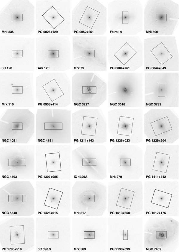
Figure 1. Final stacked images for the full sample of 35 reverberation-mapped AGNs with HST imaging. The ground-based spectroscopic monitoring apertures are overlaid. Each image is 25'' × 25'', with north up and east to the left.
Download figure:
Standard image High-resolution image2.2. MDM Observatory
Images of the reverberation-mapped sample of galaxies were also taken with the 1.3 m McGraw-Hill Telescope at MDM Observatory. Templeton, a 1024 × 1024 pixel CCD, was employed for the observations, giving a field of view (FOV) of 8 53 × 853 and a pixel scale of 050 pixel−1. Each galaxy was imaged through Harris B, V, and R filters. We focus here on the observations of the seven NGC objects that were visible from the location of MDM Observatory8. A log of the MDM observations for those objects is presented in Table 3. The data were reduced and combined with IRAF9 following standard procedures. The final V-band images are shown in Figure 2.

Figure 2. V-band images of the seven NGC objects in the reverberation-mapped sample that are visible from MDM Observatory. Each image is 5' × 5', with north up and east to the left.
Download figure:
Standard image High-resolution imageTable 3. MDM Observation Log
| Exposure Times | ||||||
|---|---|---|---|---|---|---|
| Object | Date Observed (yyyy-mm-dd) | Air Mass (sec z) | B (s) | V (s) | R (s) | Seeing ('') |
| NGC 3227 | 2003-02-08 | 1.023–1.135 | 1800 | 1680 | 795 | 1.77 |
| NGC 3516 | 2003-04-25 | 1.317–1.392 | 1900 | 845 | 1500 | 1.85 |
| NGC 4051 | 2003-02-08 | 1.048–1.111 | 1250 | 795 | 690 | 1.71 |
| NGC 4151 | 2003-02-09 | 1.008–1.050 | 1470 | 1200 | 1220 | 2.07 |
| NGC 4593 | 2003-02-09 | 1.298–1.576 | 1650 | 1860 | 1380 | 2.58 |
| NGC 5548 | 2003-04-25 | 1.018–1.308 | 4000 | 2500 | 1080 | 1.63 |
| NGC 7469 | 2003-09-26 | 1.087–1.106 | 1440 | 1260 | 1560 | 1.69 |
Download table as: ASCIITypeset image
3. GALAXY DECOMPOSITIONS
The images of each of the objects were modeled with typical galaxy parameters in order to determine and accurately subtract the contribution from the central point source. The models were constructed using the two-dimensional image decomposition program Galfit (Peng et al. 2002), which fits analytic functions for the components of the galaxy, plus an additional point source for the nucleus, convolved with a user-supplied model PSF.
For each of the objects in this study, the final cleaned, stacked image was fit with a central PSF and a constant sky contribution, as well as host-galaxy components that were modeled using variations of the Sersic (1968) profile,

where re is the effective radius of the component, Σe is the surface brightness at re, n is the power-law index, and κ is coupled to n such that half of the total flux is within re. Two special cases of the Sérsic function are the exponential profile (n = 1), often used in modeling galactic disks, and the de Vaucouleurs (1948) profile (n = 4), historically used for modeling galactic bulges. We modeled disk components using the exponential profile. However, we improve upon the results presented by Bentz et al. (2006a) in that we employed the more general Sérsic function for modeling bulges and we allow for additional parameters to describe other surface brightness components (such as a bar or inner bulge component). These modifications were partially prompted by the large body of observations that find disk galaxies (of which our sample is mostly comprised) are more accurately described with bulge profiles that have n < 4 (e.g., Kormendy & Bruzual 1978; Shaw & Gilmore 1989; Andredakis & Sanders 1994; MacArthur et al. 2008).
There is a paucity of archival stellar images with the HRC through the F550M filter, and so simulated PSFs were created using the TinyTim package (Krist 1993) which models the optics of HST plus the specifics of the camera and filter system. We tested our fits using a white dwarf image from the HST archive as the PSF model (GO 10752, PI: Lallo). Unfortunately, the image did not have the extremely high dynamic range necessary for a good fit when compared to these bright AGNs.
Many of the nearest galaxies in this sample fill the FOV of the ACS HRC, and so the sky contribution could not simply be measured from the edges of the images. Rather, the sky level was iteratively determined, starting with an estimate of the sky brightness from the ACS Instrument Handbook as the initial input. The sky value was held fixed while additional parameters were fit to the galaxy. If the estimated sky value was too low, the Sérsic index for the bulge would run up to the maximum allowed value, punching a "hole" in the nucleus of the image. If the estimated sky value was too high, the Sérsic index could run down to zero, causing Galfit to crash. A sky value intermediate to these two situations was chosen such that the residuals and χ2 values were minimized. Once a preliminary fit was achieved, the sky value was checked and adjusted if necessary, after which the galaxy parameters were re-fit. This is an improvement over our previous work, where the sky contribution was assumed to be negligible compared to the bright host galaxies of the 14 AGNs in that sample, especially as our expanded sample includes several AGNs that are significantly brighter than their host galaxies.
All of the images required at least one galaxy component in addition to the sky and central PSF. Most required two, and a few required three or more to fit an additional component, such as a bar. Several of the bright AGNs required a small (less than 2 pixel effective radius) component to help account for PSF mismatch between the AGN and the model PSF (for a full discussion of PSF variations and mismatches in HST imaging, see Krist 2003 and Kim et al 2008). Extraneous objects in the field were also fit, such as intervening stars or galaxies, to ensure that the proper distribution of light was attributed to the AGN host galaxy. Compared to the simple galaxy decompositions for the 14 objects in our previous work, the surface brightness residuals and nominal χ2 fitting values have been significantly reduced, showing that the fits presented here more accurately model the underlying host-galaxy surface brightness distributions. For example, the average magnitude of the residuals for 3C 120 was reduced by a factor of ∼4 and the χ2 value10 was reduced by a factor of ∼5. In all cases, the fits have been encouraged to attribute more flux to the sky background and PSF components, resulting in conservative flux values for the host-galaxy components. The quoted brightness for each of the host-galaxy components may be somewhat underestimated as a result.
For the seven NGC objects with MDM images, the V-band MDM images were each fit with an exponential disk and a Sérsic bulge. The effective radius of the disk component was then translated to the pixel scale of the HRC camera and held fixed during the fits to the HST image. As the seeing in the MDM images was typically on the order of ∼2'', the PSF and the bulge of the galaxy were blurred together. Thus, the bulge fits from the ground-based images were held to be unreliable and were instead determined from the HST images.
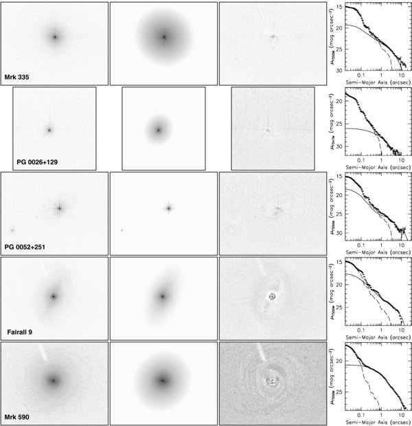
Table 4 presents the details of the fits to the HST images. The input image, Galfit model, residuals, and one-dimensional surface brightness cut for each of the 35 host galaxies are presented in Figure 3(a). Global parameters including the total galaxy luminosity and the ratio of the bulge luminosity to the total luminosity (B/T) were determined from the fits and are listed in Table 5. Also listed in Table 5 are the morphological classifications of the galaxies, several of which were listed in the NASA/IPAC Extragalactic Database (NED). For those objects without morphological classifications (objects marked with a flag in Table 5), the parameters fit to the galaxy images were used to determine the appropriate classification based on the de Vaucouleurs (1959) classification scheme. The index k for the subtype of the elliptical galaxies in the sample was calculated as k = 10(1 − b/a) and rounded to the nearest whole number. Spiral galaxies were classified based on their B/T compared to the mean of the distributions of B/T as a function of morphological type in Figure 6 of Kent (1985).
Download figure:
Standard image High-resolution image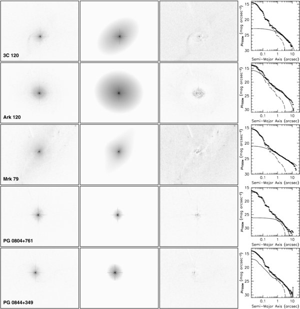
Download figure:
Standard image High-resolution image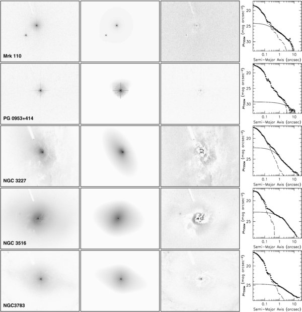
Download figure:
Standard image High-resolution image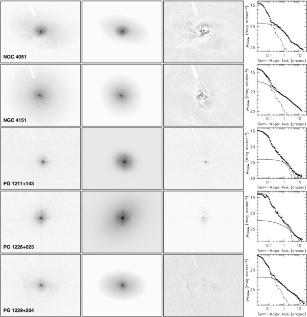
Download figure:
Standard image High-resolution image
Download figure:
Standard image High-resolution image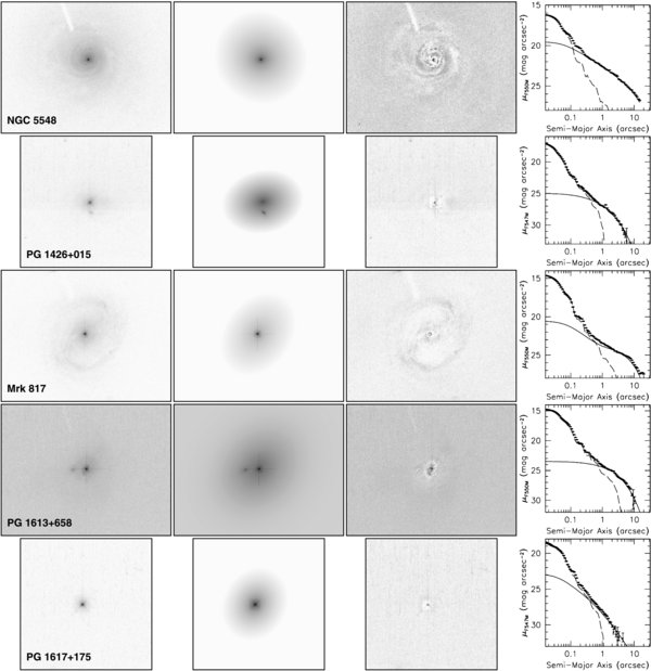
Download figure:
Standard image High-resolution image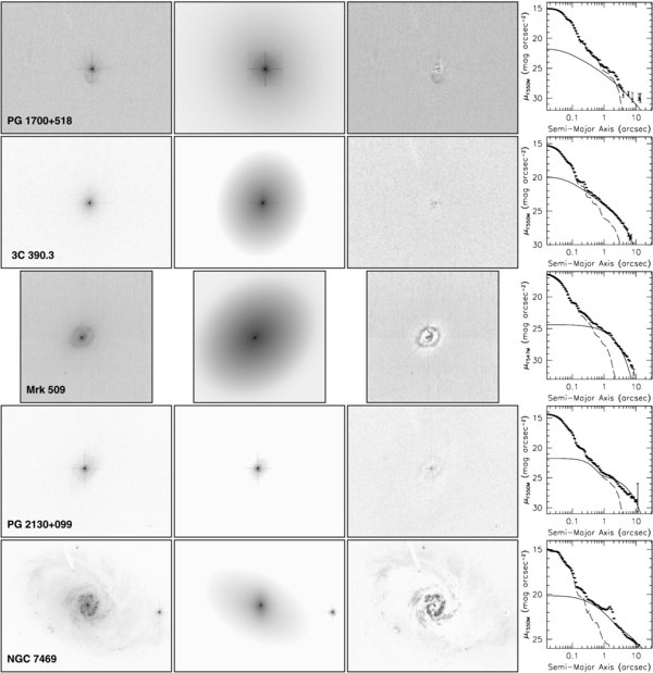
Figure 3. From left to right, each row shows the following: the HST image of an AGN and its host galaxy; the best fit to the galaxy+AGN surface brightness profiles from Galfit; the residuals of the fit; isophotal analysis of the image and models, with the data points measured from the sky-subtracted HST image, the solid line from the total host-galaxy model image (which is convolved with the PSF for comparison with the observed image), and the dashed line from the PSF model for the AGN component.
Download figure:
Standard image High-resolution imageTable 4. Details of Galaxy Fits
| Object | Sky (counts) | mstmaga | Re (kpc) | n | b/a | Note |
|---|---|---|---|---|---|---|
| Mrk 335 | 10.0 | 14.9 | PSF | |||
| 16.3 | 0.51 | 6.61 | 0.84 | Bulge | ||
| 15.8 | 1.49 | 1.00 | 0.95 | Disk | ||
| PG 0026+129 | 2.8 | 16.1 | PSF | |||
| 17.0 | 0.16 | 2.58 | 0.52 | Add'l PSF | ||
| 17.3 | 7.21 | 1.72 | 0.86 | Bulge | ||
| PG 0052+251 | 5.7 | 15.6 | PSF | |||
| 18.0 | 0.17 | 3.12 | 0.34 | Bulge | ||
| 17.2 | 8.24 | 1.00 | 0.69 | Disk | ||
| 18.8 | 3.77 | 5.47 | 0.78 | Field galaxy | ||
| Fairall 9 | 7.0 | 15.1 | PSF | |||
| 15.3 | 0.49 | 5.61 | 0.94 | Bulge | ||
| 15.3 | 2.92 | 1.00 | 0.44 | Disk | ||
| Mrk 590 | 6.8 | 17.9 | PSF | |||
| 16.3 | 0.44 | 1.22 | 0.62 | Inner bulge | ||
| 15.8 | 0.75 | 0.59 | 0.96 | Bulge | ||
| 14.2 | 3.14 | 1.00 | 0.91 | Disk | ||
| 3C 120 | 8.0 | 14.9 | PSF | |||
| 18.3 | 0.04 | 3.67 | 0.10 | Add'l PSF | ||
| 17.6 | 0.66 | 1.10 | 0.89 | Bulge | ||
| 16.1 | 3.11 | 1.00 | 0.65 | Disk | ||
| Ark 120 | 12.3 | 14.7 | PSF | |||
| 15.0 | 0.05 | 3.62 | 0.84 | Bulge | ||
| 14.9 | 1.85 | 1.00 | 0.87 | Disk | ||
| Mrk 79 | 13.7 | 15.7 | PSF | |||
| 16.1 | 0.85 | 2.79 | 0.67 | Bulge | ||
| 16.6 | 1.98 | 1.00 | 0.66 | Disk | ||
| 14.7 | 8.89 | 0.55 | 0.24 | Bar | ||
| PG 0804+761 | 10.7 | 15.0 | PSF | |||
| 14.7 | 0.08 | 1.22 | 0.73 | Add'l PSF | ||
| 16.8 | 3.33 | 1.00 | 0.74 | Bulge | ||
| PG 0844+349 | 6.0 | 14.6 | PSF | |||
| 16.9 | 0.04 | 2.28 | 0.12 | Bulge | ||
| 16.7 | 2.86 | 1.00 | 0.75 | Disk | ||
| Mrk 110 | 3.7 | 16.1 | PSF | |||
| 18.2 | 0.25 | 1.35 | 0.85 | Bulge | ||
| 16.5 | 1.73 | 1.00 | 0.93 | Disk | ||
| 16.6 | Star | |||||
| NGC 3227 | 14.2 | 15.2 | PSF | |||
| 15.4 | 0.01 | 1.51 | 0.92 | Add'l PSF | ||
| 14.9 | 0.06 | 1.08 | 0.68 | Inner bulge | ||
| 12.8 | 1.19 | 2.14 | 0.50 | Bulge | ||
| 13.8 | 4.66 | 1.00 | 0.47 | Disk | ||
| NGC 3516 | 12.0 | 15.2 | PSF | |||
| 13.4 | 0.38 | 1.24 | 0.77 | Inner bulge | ||
| 13.0 | 1.74 | 0.96 | 0.60 | Bulge | ||
| 14.4 | 4.53 | 1.00 | 0.52 | Disk | ||
| PG 0953+414 | 10.0 | 14.9 | PSF | |||
| 17.7 | 28.82 | 1.39 | 0.55 | Bulge | ||
| NGC 3783 | 12.0 | 14.2 | PSF | |||
| 14.7 | 0.49 | 1.09 | 0.92 | Bulge | ||
| 15.0 | 1.95 | 0.33 | 0.29 | Bar | ||
| 12.0 | 6.02 | 1.00 | 0.83 | Disk | ||
| NGC 4051 | 8.0 | 14.8 | PSF | |||
| 15.1 | 0.03 | 1.07 | 0.85 | Inner bulge | ||
| 15.1 | 0.07 | 0.31 | 0.71 | Inner bulge | ||
| 12.8 | 0.86 | 1.80 | 0.49 | Bulge | ||
| 12.4 | 4.24 | 1.00 | 0.67 | Disk | ||
| NGC 4151 | 0.2 | 14.5 | PSF | |||
| 14.4 | 0.07 | 4.29 | 0.54 | Inner bulge | ||
| 14.0 | 0.14 | 0.71 | 0.96 | Inner bulge | ||
| 12.0 | 0.73 | 0.81 | 0.95 | Bulge | ||
| 13.0 | 3.77 | 1.00 | 0.69 | Disk | ||
| PG 1211+143 | 17.0 | 22.5 | PSF | |||
| 14.9 | 0.06 | 0.08 | 0.63 | Add'l PSF | ||
| 17.3 | 2.59 | 1.00 | 0.84 | Bulge | ||
| PG 1226+023 | 6.5 | 15.4 | PSF | |||
| 13.2 | 0.14 | 0.22 | 0.29 | Add'l PSF | ||
| 15.6 | 11.71 | 2.50 | 0.75 | Bulge | ||
| PG 1229+204 | 15.6 | 16.7 | PSF | |||
| 20.2 | 0.23 | 0.82 | 0.69 | Bar? | ||
| 17.3 | 0.99 | 1.15 | 0.87 | Bulge | ||
| 15.8 | 7.84 | 1.00 | 0.62 | Disk | ||
| NGC 4593 | 15.0 | 15.3 | PSF | |||
| 15.1 | 0.52 | 0.09 | 0.71 | Inner bulge | ||
| 12.3 | 2.83 | 1.94 | 0.68 | Bulge | ||
| 13.5 | 9.68 | 1.00 | 0.52 | Disk | ||
| PG 1307+085 | 1.3 | 15.6 | PSF | |||
| 18.1 | 0.19 | 0.43 | 0.05 | Add'l PSF | ||
| 17.6 | 8.74 | 1.25 | 0.80 | Bulge | ||
| IC 4329A | 15.0 | 14.6 | PSF | |||
| 13.8 | 0.01 | 0.31 | 0.87 | Add'l PSF | ||
| 13.7 | 0.77 | 0.39 | 0.96 | Inner bulge | ||
| 12.6 | 3.36 | 0.50 | 0.43 | Bulge | ||
| 15.8 | 8.74 | 1.00 | 0.41 | Disk | ||
| Mrk 279 | 6.0 | 15.0 | PSF | |||
| 16.2 | 0.05 | 5.94 | 0.65 | Inner bulge | ||
| 16.2 | 0.97 | 1.88 | 0.60 | Bulge | ||
| 15.2 | 3.14 | 1.00 | 0.54 | Disk | ||
| PG 1411+442 | 9.3 | 15.7 | PSF | |||
| 15.8 | 0.05 | 1.00 | 0.48 | Add'l PSF | ||
| 16.8 | 5.05 | 1.71 | 0.58 | Bulge | ||
| 18.8 | 1.87 | 2.23 | 0.64 | Field galaxy | ||
| NGC 5548 | 0.2 | 16.7 | PSF | |||
| 14.7 | 1.18 | 4.36 | 0.86 | Inner bulge | ||
| 13.8 | 2.95 | 1.39 | 0.90 | Bulge | ||
| 15.5 | 11.51 | 1.00 | 0.85 | Disk | ||
| PG 1426+015 | 1.8 | 15.2 | PSF | |||
| 16.3 | 4.74 | 1.63 | 0.77 | Bulge | ||
| 19.8 | 0.91 | 3.14 | 0.56 | Field galaxy | ||
| 21.7 | 0.15 | 1.98 | 0.50 | Field galaxy | ||
| Mrk 817 | 4.7 | 15.1 | PSF | |||
| 17.7 | 0.28 | 2.44 | 0.81 | Bulge | ||
| 14.4 | 4.32 | 1.00 | 0.74 | Disk | ||
| PG 1613+658 | 11.0 | 15.2 | PSF | |||
| 16.3 | 6.75 | 1.35 | 0.80 | Bulge | ||
| 19.1 | 1.79 | 3.64 | 0.60 | Field galaxy | ||
| PG 1617+175 | 1.3 | 16.3 | PSF | |||
| 17.4 | 0.15 | 0.09 | 0.07 | Add'l PSF | ||
| 17.3 | 3.28 | 5.35 | 0.84 | Bulge | ||
| PG 1700+518 | 9.0 | 19.2 | PSF | |||
| 15.3 | 0.15 | 0.02 | 0.58 | Add'l PSF | ||
| 16.9 | 0.28 | 0.37 | 0.65 | Add'l PSF | ||
| 17.7 | 12.06 | 5.61 | 0.89 | Bulge | ||
| 3C 390.3 | 1.3 | 15.8 | PSF | |||
| 17.0 | 0.77 | 3.86 | 0.74 | Bulge | ||
| 16.9 | 2.54 | 1.00 | 0.86 | Disk | ||
| Mrk 509 | 4.2 | 14.5 | PSF | |||
| 15.4 | 0.04 | 0.03 | 0.48 | Add'l PSF | ||
| 15.0 | 1.85 | 1.00 | 0.79 | Bulge | ||
| PG 2130+099 | 4.0 | 14.8 | PSF | |||
| 18.9 | 0.38 | 0.56 | 0.37 | Bulge | ||
| 16.5 | 4.66 | 1.00 | 0.55 | Disk | ||
| NGC 7469 | 7.0 | 15.2 | PSF | |||
| 15.0 | 0.37 | 1.37 | 0.70 | Inner bulge | ||
| 13.4 | 3.68 | 1.31 | 0.55 | Bulge | ||
| 14.6 | 6.99 | 1.00 | 0.94 | Disk | ||
| 16.2 | Star |
Note.
aThe magnitude of an object is computed as  , where zpt = 24.457 for the F550M filter with ACS HRC and zpt = 21.685 for the F547M filter with the PC chip on WFPC2.
Table 5. Global Galaxy Parameters
| B/T | |||||
|---|---|---|---|---|---|
| Object | λLλ,gal(5100 Å)a (1044 erg s−1) | 1 | 2c | Morphological Classification | Flagb |
| Mrk 335 | 0.37 | 0.37 | S0/a | ||
| PG 0026+129 | 2.3 | 1.00 | E1 | * | |
| PG 0052+251 | 4.1 | 0.32 | Sb | ||
| Fairall 9 | 2.4 | 0.52 | SBa | * | |
| Mrk 590 | 1.4 | 0.17 | 0.28 | SA(s)a | |
| 3C 120 | 0.73 | 0.21 | S0 | ||
| Akn 120 | 2.1 | 0.49 | Sb pec | ||
| Mrk 79 | 0.73 | 0.19 | 0.87 | SBb | |
| PG 0804+761 | 1.5 | 1.00 | E3 | * | |
| PG 0844+349 | 1.2 | 0.45 | Sa | * | |
| Mrk 110 | 0.26 | 0.17 | Sc | * | |
| PG 0953+414 | 3.6 | 1.00 | E4 | * | |
| NGC 3227 | 0.23 | 0.65 | 0.74 | SAB(s) pec | |
| NGC 3516 | 0.69 | 0.52 | 0.86 | (R)SB(s) | |
| NGC 3783 | 1.5 | 0.07 | 0.12 | (R')SB(r)a | |
| NGC 4051 | 0.16 | 0.36 | 0.45 | SAB(rs)bc | |
| NGC 4151 | 0.20 | 0.60 | 0.75 | (R')SAB(rs)ab | |
| PG 1211+143 | 0.59 | 1.00 | E2 | * | |
| PG 1226+023 | 11.3 | 1.00 | E3 | * | |
| PG 1229+204 | 1.8 | 0.20 | 0.21 | SBc | * |
| NGC 4593 | 0.91 | 0.71 | 0.76 | (R)SB(rs)b | |
| PG 1307+085 | 1.8 | 1.00 | E2 | * | |
| IC 4329A | 2.4 | 0.70 | 0.96 | SA0 | |
| Mrk 279 | 0.95 | 0.21 | 0.43 | S0 | |
| PG 1411+442 | 1.2 | 1.00 | E4 | * | |
| NGC 5548 | 0.98 | 0.60 | 0.87 | (R')SA(s)0/a | |
| PG 1426+015 | 1.8 | 1.00 | E2 | * | |
| Mrk 817 | 1.2 | 0.05 | SBc | ||
| PG 1613+658 | 4.2 | 1.00 | E2 | * | |
| PG 1617+175 | 1.3 | 1.00 | E2 | * | |
| PG 1700+518 | 6.7 | 1.00 | E1 | * | |
| 3C 390.3 | 0.87 | 0.48 | Sa | * | |
| Mrk 509 | 0.95 | 1.00 | E2 | * | |
| PG 2130+099 | 0.88 | 0.10 | (R)Sa | ||
| NGC 7469 | 1.4 | 0.64 | 0.79 | (R')SAB(rs)a | |
Notes. aGalaxy luminosities are determined directly from the model parameters that were fit to the HST images. They do not include features that were not modeled, such as the nuclear starburst ring in NGC 7469, and do not include the contributions from field galaxies or stars. bMorphological classifications are from NED where available. Those marked with a flag are determined from the galaxy fit parameters in this work, as described in the text. cBulge luminosities here include the contribution from any bar and/or inner bulge component.
Download table as: ASCIITypeset image
As discussed by Peng et al. (2002), degeneracy between galaxy components and between parameters within components is typically an issue when fitting analytic models to galaxy images. This is certainly the case with the sample of objects presented here. The bright AGNs in the galaxy centers are degenerate with the concentration of the bulge (the Sérsic index n), especially when the bulge component is rather compact. As discussed above, many of these images have the added complication of having a somewhat uncertain sky contribution which also affects n as well as the scale length of the disk. Interpreting the specific details of the galaxy fits presented here is therefore difficult. The relatively low n values for the galaxy bulges in this sample certainly seem to agree with the works referenced above that find n < 4 for most spiral galaxies. However, the actual n values may be somewhat underestimated as a result of our conservative fits that attribute more flux to the AGN and the sky background. A quick glance through the galaxy fits in Table 4 might lead one to speculate on the prevalence of pseudobulges versus classical bulges in this sample. As per the discussion by Kormendy & Kennicutt (2004), however, the lack of dynamical information for the host galaxies in this sample as well as the uncertainty in interpreting the galaxy fitting parameters complicates any conclusions that might be drawn about the origins of the bulges in these galaxies.
Several of the fits listed in Table 4 include components noted as being an "inner bulge" or "bar." The classifications for these extra components are simply morphological, with a "bar" typically having a more elongated shape than an "inner bulge." Bars themselves tend to have an inner bulbous component, so the "inner bulges" listed here may actually be related to bars themselves (Peng et al. 2002). We do not have kinematic information to determine which of these additional components may be physically distinct from the bulge or disk of the host galaxy. The fact that additional components are required to achieve a better fit is likely in many cases to simply be the result of attempting to fit analytic functions to resolved galaxies with strong substructure. In particular, areas with dust obscuration and spiral arm structure are difficult to properly fit with analytic functions. As our main goal is to determine the PSF contribution as accurately as possible and to create "nucleus-free" images of these galaxies, we do not discuss here the origin or meaning of these additional components in the galaxy fits.
In Table 6, we list a comparison of the fitting results for the objects and monitoring apertures that were examined by Bentz et al. (2006a). As can easily be seen, the χ2/ν decreased for all the objects except Mrk 279 using the fitting scheme outlined in this work. As the particular value of χ2/ν can be somewhat misleading due to the number of degrees of freedom not being the same between the two fits for each object, we also present the mean and standard deviation of the fitting residuals for each object. In all cases, the mean of the residuals is now much closer to zero and the standard deviation is much smaller than it was before, clearly showing that the fits presented here more accurately model the actual surface brightness distribution of the AGN host galaxies. Finally, we also list the galaxy flux in counts per second as measured through the ground-based monitoring apertures listed in our previous work (some of which are not included here due to updated monitoring programs; see Section 4) and the ratio of the new galaxy flux to the old galaxy flux, which has an average value of 0.78 ± 0.20 due solely to the image fitting procedure. This ratio may be slightly exaggerated, as we have purposefully carried out conservative fits to the galaxy images in this work.
Table 6. Comparison of Galaxy Fitting Results
| Bentz et al. (2006a) | This Work | ||||||
|---|---|---|---|---|---|---|---|
| Object | χ2/ν | Image−Model (counts) | fgal (counts s−1) | χ2/ν | Image−Model (counts) | fgal (counts s−1) |  |
| 3C 120 | 4.8 | 1.3 ± 344 | 2905.1 | 1.5 | −1 ± 110 | 1314.0 | 0.45 |
| 3C 390.3 | 2.7 | 0.8 ± 128 | 1951.3 | 1.3 | −1 ± 32 | 1584.4 | 0.81 |
| Fairall 9 | 2.7 | 2.3 ± 187 | 7407.2 | 2.9 | 0 ± 231 | 5828.3 | 0.79 |
| Mrk 110 | 2.8 | 0.9 ± 115 | 1728.3 | 1.3 | 0 ± 38 | 1318.1 | 0.76 |
| Mrk 279 | 4.8 | 1.6 ± 333 | 5969.7 | 11.3 | 1 ± 320 | 5849.3 | 0.98 |
| Mrk 590 | 8.6 | 1.3 ± 24 | 8473.9 | 8.2 | 1 ± 12 | 8067.1 | 0.95 |
| Mrk 817 | 12.0 | 1.8 ± 230 | 4015.6 | 10.0 | 1 ± 102 | 2974.2 | 0.74 |
| NGC 3227 | 19.2 | 8.6 ± 263 | 9877.8 | 9.4 | 1 ± 97 | 6915.4 | 0.70 |
| NGC 3783 | 18.0 | 5.9 ± 763 | 12696.8 | 8.0 | 2 ± 375 | 10164.8 | 0.80 |
| NGC 4051 | 14.7 | 4.9 ± 340 | 17644.9 | 6.7 | 1 ± 81 | 16967.6 | 0.96 |
| NGC 4151 | 17.6 | 10.1 ± 378 | 51822.3 | 6.6 | 1 ± 194 | 51559.6 | 0.99 |
| NGC 5548 | 11.8 | 1.2 ± 54 | 7739.0 | 11.6 | 1 ± 19 | 7764.0 | 1.00 |
| PG 0844+761 | 6.8 | 2.1 ± 470 | 4367.0 | 3.0 | 0 ± 330 | 2075.4 | 0.48 |
| PG 2130+099 | 5.6 | 1.3 ± 400 | 3215.7 | 1.5 | 0 ± 84 | 1480.0 | 0.46 |
Notes. When comparing the χ2/ν values listed above, it should be remembered that the degrees of freedom (ν) in each fit depends on the number of surface brightness model parameters included. The galaxy fluxes listed are measured through the ground-based monitoring apertures presented by Bentz et al. (2006a), some of which are not included in this work as discussed in Section 4.
Download table as: ASCIITypeset image
4. FLUX MEASUREMENTS
Once the fit to each galaxy was finalized, the sky and PSF components were subtracted, leaving a nucleus-free image of each host galaxy. Each image was overlaid with the typical aperture used in the ground-based monitoring program(s), at the typical orientation and centered on the position of the AGN (see Table 7). The counts within the aperture were summed and converted to fλ flux density units (erg s−1 cm−2 Å−1) using the HST keyword PHOTFLAM and the effective exposure time for each object.
Table 7. Ground-Based Monitoring Apertures and Observed Fluxes
| Object | Referencea | P.A. (°) | Aperture ('' × '') | f((1 + z) 5100 Å) (10−15 erg s−1 cm−2 å−1) |
|---|---|---|---|---|
| Mrk 335 | 1 | 90.0 | 5.0 × 7.6 | 7.68 ± 0.53 |
| 1 | 90.0 | 5.0 × 7.6 | 8.81 ± 0.47 | |
| PG 0026+129 | 2 | 42.0 | 10.0 × 13.0 | 2.69 ± 0.40 |
| PG 0052+251 | 2 | 153.4 | 10.0 × 13.0 | 2.07 ± 0.37 |
| Fairall 9 | 3 | 0.0 | 4.0 × 9.0 | 5.95 ± 0.66 |
| Mrk 590 | 1 | 90.0 | 5.0 × 7.6 | 7.89 ± 0.62 |
| 1 | 90.0 | 5.0 × 7.6 | 5.33 ± 0.56 | |
| 1 | 90.0 | 5.0 × 7.6 | 6.37 ± 0.45 | |
| 1 | 90.0 | 5.0 × 7.6 | 8.43 ± 1.30 | |
| 3C 120 | 1 | 90.0 | 5.0 × 7.6 | 4.30 ± 0.77 |
| Akn 120 | 1 | 90.0 | 5.0 × 7.6 | 10.37 ± 0.46 |
| 1 | 90.0 | 5.0 × 7.6 | 7.82 ± 0.83 | |
| Mrk 79 | 1 | 90.0 | 5.0 × 7.6 | 6.96 ± 0.67 |
| 1 | 90.0 | 5.0 × 7.6 | 8.49 ± 0.86 | |
| 1 | 90.0 | 5.0 × 7.6 | 7.40 ± 0.72 | |
| PG 0804+761 | 2 | 315.6 | 10.0 × 13.0 | 5.48 ± 1.00 |
| PG 0844+349 | 2 | 36.8 | 10.0 × 13.0 | 3.71 ± 0.38 |
| Mrk 110 | 1 | 90.0 | 5.0 × 7.6 | 3.45 ± 0.36 |
| 1 | 90.0 | 5.0 × 7.6 | 3.96 ± 0.51 | |
| 1 | 90.0 | 5.0 × 7.6 | 2.64 ± 0.86 | |
| PG 0953+414 | 2 | 31.7 | 10.0 × 13.0 | 1.56 ± 0.21 |
| NGC 3227 | 4 | 25.0 | 1.5 × 4.0 | 23.46 ± 3.70 |
| 5 | 90.0 | 5.0 × 10.0 | 12.70 ± 0.68 | |
| NGC 3516 | 6 | 25.0 | 1.5 × 2.0 | 7.83 ± 2.35 |
| NGC 3783 | 7 | 0.0 | 5.0 × 10.0 | 11.38 ± 0.95 |
| NGC 4051 | 8 | 90.0 | 5.0 × 7.5 | 13.38 ± 0.92 |
| NGC 4151 | 9 | 90.0 | 5.0 × 12.75 | 23.8 ± 3.0 |
| PG 1211+143 | 2 | 352.2 | 10.0 × 13.0 | 5.66 ± 0.92 |
| PG 1226+023 | 2 | 171.2 | 10.0 × 13.0 | 21.30 ± 2.60 |
| PG 1229+204 | 2 | 291.5 | 10.0 × 13.0 | 2.15 ± 0.23 |
| NGC 4593 | 10 | 90.0 | 5.0 × 12.75 | 15.9 ± 0.7 |
| PG 1307+085 | 2 | 186.5 | 10.0 × 13.0 | 1.79 ± 0.18 |
| IC 4329A | 11 | 90.0 | 5.0 × 10.0 | 5.79 ± 0.73 |
| Mrk 279 | 12 | 90.0 | 5.0 × 7.5 | 6.90 ± 0.69 |
| PG 1411+442 | 2 | 347.0 | 10.0 × 13.0 | 3.71 ± 0.32 |
| NGC 5548 | 13 | 90.0 | 5.0 × 7.5 | 9.92 ± 1.26 |
| 13 | 90.0 | 5.0 × 7.5 | 7.25 ± 1.00 | |
| 13 | 90.0 | 5.0 × 7.5 | 9.40 ± 0.93 | |
| 13 | 90.0 | 5.0 × 7.5 | 6.72 ± 1.17 | |
| 13 | 90.0 | 5.0 × 7.5 | 9.06 ± 0.86 | |
| 13 | 90.0 | 5.0 × 7.5 | 9.76 ± 1.10 | |
| 13 | 90.0 | 5.0 × 7.5 | 12.09 ± 1.00 | |
| 13 | 90.0 | 5.0 × 7.5 | 10.56 ± 1.64 | |
| 13 | 90.0 | 5.0 × 7.5 | 8.12 ± 0.91 | |
| 13 | 90.0 | 5.0 × 7.5 | 13.47 ± 1.45 | |
| 13 | 90.0 | 5.0 × 7.5 | 11.83 ± 1.82 | |
| 13 | 90.0 | 5.0 × 7.5 | 6.98 ± 1.20 | |
| 13 | 90.0 | 5.0 × 7.5 | 7.03 ± 0.86 | |
| 14 | 90.0 | 5.0 × 12.75 | 6.63 ± 0.36 | |
| PG 1426+015 | 2 | 341.4 | 10.0 × 13.0 | 4.62 ± 0.71 |
| Mrk 817 | 1 | 90.0 | 5.0 × 7.6 | 6.10 ± 0.83 |
| 1 | 90.0 | 5.0 × 7.6 | 5.00 ± 0.49 | |
| 1 | 90.0 | 5.0 × 7.6 | 5.01 ± 0.27 | |
| PG 1613+658 | 2 | 164.2 | 10.0 × 13.0 | 3.49 ± 0.43 |
| PG 1617+175 | 2 | 253.0 | 10.0 × 13.0 | 1.44 ± 0.25 |
| PG 1700+518 | 2 | 183.5 | 10.0 × 13.0 | 2.20 ± 0.15 |
| 3C 390.3 | 15 | 90.0 | 5.0 × 7.5 | 1.73 ± 0.28 |
| Mrk 509 | 1 | 90.0 | 5.0 × 7.6 | 10.92 ± 1.99 |
| PG 2130+099 | 16 | 0.0 | 3.0 × 6.97 | 4.63 ± 0.23 |
| NGC 7469 | 17 | 90.0 | 5.0 × 7.5 | 13.57 ± 0.61 |
Notes. Here, and throughout, observed galaxy fluxes are tabulated at rest-frame 5100 Å. aReferences refer to reverberation-mapping campaigns in optical wavelengths. References. (1) Peterson et al. (1998); (2) Kaspi et al. (2000); (3) Santos-Lleó et al. (1997); (4) Salamanca et al. (1994); (5) Winge et al. (1995); (6) Wanders et al. (1993); (7) Stirpe et al. (1994); (8) Peterson et al. (2000); (9) Bentz et al. (2006b); (10) Denney et al. (2006); (11) Winge et al. (1996); (12) Santos-Lleó et al. (2001); (13) Peterson et al. (2002), and references therein; (14) Bentz et al. (2007); (15) Dietrich et al. (1998); (16) Grier et al. (2008); (17) Collier et al. (1998).
Color corrections to the observed galaxy flux densities were calculated using a model bulge spectrum (Kinney et al. 1996) to account for the difference between the effective wavelength of the HST filter and rest-frame 5100 Å for each object. The model bulge spectrum was redshifted to the distance of each AGN host galaxy and reddened by the appropriate Galactic extinction. The redshifted, reddened models were convolved with the HST filter response using the synphot package in the IRAF/STSDAS library and subsequently scaled to the appropriate flux level as measured from the HST images. Finally, the observed flux at rest-frame 5100 Å was measured from the model. The flux density measured directly from the nucleus-free HST images and the color-corrected flux and luminosity at 5100 Å are listed in Table 8. We note that the color correction method outlined above is different from that employed previously, and again results in more conservative host-galaxy flux values.
Table 8. Host-Galaxy Fluxes and Luminosities
| Object | fgal(HST) (10−15 erg s−1 cm−2 Å−1) |  fgal((1 + z) 5100 Å) fgal((1 + z) 5100 Å) |
fgal((1 + z) 5100 Å) (10−15 erg s−1 cm−2 Å−1) | λLλ,gal(5100 Å)a (1044 erg s−1) |
|---|---|---|---|---|
| Mrk 335 | 1.88 | 0.85 | 1.60 ± 0.15 | 0.142 ± 0.013 |
| PG 0026+129 | 0.381 | 1.00 | 0.379 ± 0.035 | 1.46 ± 0.13 |
| PG 0052+251 | 0.713 | 0.98 | 0.699 ± 0.064 | 3.08 ± 0.28 |
| Fairall 9 | 3.47 | 0.88 | 3.07 ± 0.28 | 0.927 ± 0.085 |
| Mrk 590 | 4.81 | 0.85 | 4.10 ± 0.38 | 0.384 ± 0.035 |
| 3C 120 | 0.783 | 0.82 | 0.641 ± 0.059 | 0.217 ± 0.020 |
| Akn 120 | 6.70 | 0.85 | 5.68 ± 0.52 | 1.079 ± 0.099 |
| Mrk 79 | 1.74 | 0.84 | 1.46 ± 0.13 | 0.106 ± 0.010 |
| PG 0804+761 | 0.703 | 0.97 | 0.683 ± 0.063 | 1.076 ± 0.099 |
| PG 0844+349 | 1.24 | 0.92 | 1.14 ± 0.11 | 0.684 ± 0.063 |
| Mrk 110 | 0.786 | 0.88 | 0.688 ± 0.063 | 0.109 ± 0.010 |
| PG 0953+414 | 0.208 | 1.11 | 0.231 ± 0.021 | 2.47 ± 0.23 |
| NGC 3227b | 4.12 | 0.82 | 3.37 ± 0.31 | 0.0124 ± 0.0011 |
| 8.57 | 0.82 | 7.01 ± 0.65 | 0.0258 ± 0.0024 | |
| NGC 3516 | 4.55 | 0.82 | 3.73 ± 0.34 | 0.0382 ± 0.0035 |
| NGC 3783 | 6.06 | 0.80 | 4.86 ± 0.45 | 0.0776 ± 0.0071 |
| NGC 4051 | 10.1 | 0.82 | 8.28 ± 0.76 | 0.0123 ± 0.0011 |
| NGC 4151 | 21.6 | 0.82 | 17.6 ± 1.6 | 0.0240 ± 0.0022 |
| PG 1211+143 | 0.633 | 0.95 | 0.598 ± 0.055 | 0.592 ± 0.054 |
| PG 1226+023 | 1.37 | 0.98 | 1.34 ± 0.12 | 5.741 ± 0.529 |
| PG 1229+204 | 1.48 | 0.92 | 1.36 ± 0.13 | 0.766 ± 0.071 |
| NGC 4593 | 10.7 | 0.82 | 8.85 ± 0.82 | 0.0889 ± 0.0082 |
| PG 1307+085 | 0.232 | 1.00 | 0.233 ± 0.021 | 0.986 ± 0.091 |
| IC 4329A | 4.43 | 0.83 | 3.67 ± 0.34 | 0.133 ± 0.012 |
| Mrk 279 | 3.49 | 0.87 | 3.02 ± 0.28 | 0.355 ± 0.033 |
| PG 1411+442 | 0.826 | 0.96 | 0.791 ± 0.073 | 0.904 ± 0.083 |
| NGC 5548b | 4.63 | 0.84 | 3.88 ± 0.36 | 0.143 ± 0.013 |
| 5.51 | 0.84 | 4.61 ± 0.43 | 0.169 ± 0.016 | |
| PG 1426+015 | 1.19 | 0.96 | 1.14 ± 0.11 | 1.29 ± 0.12 |
| Mrk 817 | 1.77 | 0.87 | 1.54 ± 0.14 | 0.188 ± 0.017 |
| PG 1613+658 | 1.52 | 0.98 | 1.50 ± 0.14 | 4.08 ± 0.38 |
| PG 1617+175 | 0.341 | 0.99 | 0.336 ± 0.031 | 0.701 ± 0.065 |
| PG 1700+518 | 0.246 | 1.41 | 0.347 ± 0.032 | 6.79 ± 0.63 |
| 3C 390.3 | 0.945 | 0.90 | 0.853 ± 0.079 | 0.430 ± 0.040 |
| Mrk 509 | 2.74 | 0.92 | 2.52 ± 0.23 | 0.435 ± 0.040 |
| PG 2130+099 | 0.440 | 0.92 | 0.405 ± 0.037 | 0.240 ± 0.022 |
| NGC 7469 | 10.2 | 0.83 | 8.43 ± 0.78 | 0.327 ± 0.030 |
Notes. aThe galaxy luminosities presented here are measured through the ground-based monitoring aperture directly from the PSF-subtracted HST images. Any field galaxies or stars, or additional unmodeled galaxy structures, that are included in the original ground-based spectroscopic aperture contribute to this luminosity. bThe two different entries for NGC 3227 and NGC 5548 correspond to the two different monitoring apertures that were employed during the spectroscopic monitoring programs for these objects. They are listed in the same order as in Table 6.
Download table as: ASCIITypeset image
The final step requires subtraction of the galaxy flux from the mean flux measured during a monitoring campaign, and leaves only the flux contribution from the AGN itself. The corresponding AGN luminosities were calculated and corrected for Galactic absorption using the Schlegel et al. (1998) AB values listed in NED and the extinction curve of Cardelli et al. (1989), adjusted to AV/E(B − V) = 3.1. The starlight-corrected AGN fluxes and luminosities are listed in Table 9 with their corresponding Hβ lags. The numbers in bold font are the weighted averages of multiple measurements for a particular object.
Table 9. Rest-Frame Time Lags and Starlight-Corrected Luminosities
| Object | Hβ Time Lag (days) | fAGN ((1 + z) 5100 Å) (10−15 erg s−1 cm−2 Å−1) | λLλ,AGN (5100 Å) (1044 erg s−1) |
|---|---|---|---|
| Mrk 335 | 16.8+4.8−4.2 | 6.09 ± 0.53 | 0.541 ± 0.047 |
| 12.5+6.6−5.5 | 7.21 ± 0.47 | 0.640 ± 0.041 | |
| 15.7+3.4−4.0 | 6.72 ± 0.35 | 0.603 ± 0.031 | |
| PG 0026+129 | 111.0+24.1−28.3 | 2.31 ± 0.40 | 8.9 ± 1.6 |
| PG 0052+251 | 89.8+24.5−24.1 | 1.37 ± 0.37 | 6.0 ± 1.6 |
| Fairall 9 | 17.4+3.2−4.3 | 2.88 ± 0.66 | 0.87 ± 0.20 |
| Mrk 590 | 20.7+3.5−2.7 | 3.80 ± 0.62 | 0.355 ± 0.058 |
| 14.0+8.5−8.8 | 1.23 ± 0.56 | 0.115 ± 0.053 | |
| 29.2+4.9−5.0 | 2.27 ± 0.45 | 0.212 ± 0.043 | |
| 28.8+3.6−4.2 | 4.3 ± 1.3 | 0.41 ± 0.12 | |
| 25.6+2.0−2.3 | 2.44 ± 0.30 | 0.287 ± 0.032 | |
| 3C 120 | 38.1+21.3−15.3 | 3.66 ± 0.77 | 1.24 ± 0.26 |
| Ark 120 | 47.1+8.3−12.4 | 4.69 ± 0.46 | 0.889 ± 0.088 |
| 37.1+4.8−5.4 | 2.14 ± 0.83 | 0.41 ± 0.16 | |
| 39.7+3.9−5.5 | 4.09 ± 0.40 | 0.847 ± 0.081 | |
| Mrk 79 | 9.0+8.3−7.8 | 5.50 ± 0.67 | 0.401 ± 0.049 |
| 16.1+6.6−6.6 | 7.03 ± 0.86 | 0.513 ± 0.063 | |
| 16.0+6.4−5.8 | 5.94 ± 0.72 | 0.435 ± 0.053 | |
| 15.2+3.4−5.1 | 6.03 ± 0.43 | 0.447 ± 0.031 | |
| PG 0804+761 | 146.9+18.8−18.9 | 4.8 ± 1.0 | 7.6 ± 1.6 |
| PG 0844+349a | 32.3+13.7−13.4 | 2.57 ± 0.38 | 1.54 ± 0.23 |
| Mrk 110 | 24.3+5.5−8.3 | 2.77 ± 0.36 | 0.439 ± 0.058 |
| 20.4+10.5−6.3 | 3.28 ± 0.51 | 0.520 ± 0.080 | |
| 33.3+14.9−10.0 | 1.95 ± 0.86 | 0.31 ± 0.14 | |
| 25.5+4.2−5.6 | 2.83 ± 0.28 | 0.461 ± 0.045 | |
| PG 0953+414 | 150.1+21.6−22.6 | 1.33 ± 0.21 | 14.2 ± 2.2 |
| NGC 3227 | 8.2+5.1−8.4 | 20.1 ± 3.7 | 0.074 ± 0.014 |
| 5.4+14.1−8.7 | 5.70 ± 0.68 | 0.0209 ± 0.0025 | |
| 7.8+3.5−10.2 | 6.17 ± 0.67 | 0.0304 ± 0.0031 | |
| NGC 3516 | 6.7+6.8−3.8 | 4.1 ± 2.3 | 0.042 ± 0.024 |
| NGC 3783 | 10.2+3.3−2.3 | 6.52 ± 0.95 | 0.104 ± 0.015 |
| NGC 4051 | 5.8+2.6−1.8 | 5.10 ± 0.92 | 0.0076 ± 0.0014 |
| NGC 4151 | 6.6+1.1−0.8 | 6.2 ± 3.0 | 0.0084 ± 0.0041 |
| PG 1211+143 | 93.8+25.6−42.1 | 5.06 ± 0.92 | 5.00 ± 0.91 |
| PG 1226+032 | 306.8+68.5−90.9 | 20.0 ± 2.6 | 86 ± 11 |
| PG 1229+204 | 37.8+27.6−15.3 | 0.79 ± 0.23 | 0.45 ± 0.13 |
| NGC 4593 | 3.7+0.8−0.8 | 7.05 ± 0.70 | 0.0708 ± 0.0070 |
| PG 1307+085 | 105.6+36.0−46.6 | 1.56 ± 0.18 | 6.59 ± 0.77 |
| IC 4329Ab | 1.5+2.7−1.8 | 2.12 ± 0.73 | 0.077 ± 0.026 |
| Mrk 279 | 16.7+3.9−3.9 | 3.88 ± 0.69 | 0.456 ± 0.082 |
| PG 1411+442 | 124.3+61.0−61.7 | 2.92 ± 0.32 | 3.34 ± 0.36 |
| NGC 5548 | 19.7+1.5−1.5 | 6.0 ± 1.3 | 0.222 ± 0.047 |
| 18.6+2.1−2.3 | 3.4 ± 1.0 | 0.124 ± 0.037 | |
| 15.9+2.9−2.5 | 5.52 ± 0.93 | 0.203 ± 0.034 | |
| 11.0+1.9−2.0 | 2.8 ± 1.2 | 0.105 ± 0.043 | |
| 13.0+1.6−1.4 | 5.19 ± 0.86 | 0.191 ± 0.032 | |
| 13.4+3.8−4.3 | 5.9 ± 1.1 | 0.216 ± 0.040 | |
| 21.7+2.6−2.6 | 8.2 ± 1.0 | 0.302 ± 0.037 | |
| 16.4+1.2−1.1 | 6.7 ± 1.6 | 0.246 ± 0.060 | |
| 17.5+2.0−1.6 | 4.25 ± 0.91 | 0.156 ± 0.033 | |
| 26.5+4.3−2.2 | 9.6 ± 1.5 | 0.352 ± 0.054 | |
| 24.8+3.2−3.0 | 8.0 ± 1.8 | 0.292 ± 0.067 | |
| 6.5+5.7−3.7 | 3.1 ± 1.2 | 0.114 ± 0.044 | |
| 14.3+5.9−7.3 | 3.16 ± 0.86 | 0.116 ± 0.032 | |
| 6.3+2.6−2.3 | 2.02 ± 0.36 | 0.074 ± 0.013 | |
| 18.0+0.6−0.6 | 3.84 ± 0.23 | 0.205 ± 0.011 | |
| PG 1426+015 | 95.0+29.9−37.1 | 3.48 ± 0.71 | 3.94 ± 0.81 |
| Mrk 817 | 19.0+3.9−3.7 | 4.56 ± 0.83 | 0.56 ± 0.10 |
| 15.3+3.7−3.5 | 3.46 ± 0.49 | 0.423 ± 0.060 | |
| 33.6+6.5−7.6 | 3.47 ± 0.27 | 0.424 ± 0.032 | |
| 21.8+2.4−3.0 | 3.54 ± 0.23 | 0.438 ± 0.028 | |
| PG 1613+658 | 40.1+15.0−15.2 | 1.99 ± 0.43 | 5.4 ± 1.2 |
| PG 1617+175 | 71.5+29.6−33.7 | 1.10 ± 0.25 | 2.30 ± 0.51 |
| PG 1700+518 | 251.8+45.9−38.8 | 1.85 ± 0.15 | 36.3 ± 2.9 |
| 3C 390.3 | 23.6+6.2−6.7 | 0.88 ± 0.28 | 0.44 ± 0.14 |
| Mrk 509 | 79.6+6.1−5.4 | 8.4 ± 2.0 | 1.45 ± 0.34 |
| PG 2130+099 | 22.9+4.7−4.6 | 4.22 ± 0.23 | 2.51 ± 0.14 |
| NGC 7469 | 4.5+0.7−0.8 | 5.14 ± 0.61 | 0.200 ± 0.023 |
Notes. Numbers in boldface are the weighted averages of all the measurements for that particular object. Fluxes are as observed. Time lags and luminosities are listed in the rest-frame of the object with weighted averages calculated in log space. aThe Hβ lag measurement for this object was deemed unreliable by Peterson et al. (2004). In its place, we give the most reliably measured lag, which is for Hα. bBecause of the extremely poor lag measurement (which is consistent with zero) and the poor flux calibration for this object, we do not include it in the fit to the RBLR–L relationship.
Ongoing work with this sample of objects has resulted in some updates to the reverberation database presented by Peterson et al. (2004) and fit by Kaspi et al. (2005). In addition, a few data sets require cautionary or explanatory notes. Specifically, we note the following.
- 1.NGC 3516. The light curves presented by Wanders et al. (1993) were not measured from data with an absolute flux calibration. Therefore, while we have included this object, it should be regarded with caution as the spectroscopic luminosity is not well determined.
- 2.NGC 4151. The aperture used in the monitoring campaign described by Maoz et al. (1991) is 20'' × 28'', which is larger than the FOV of the HRC camera. In addition, the Kaspi et al. (1996) data set has a rather unconstrained time lag that is consistent with zero once the monotonic increase in the continuum and line flux is removed (see Metzroth et al. 2006 for a full discussion). Both of these data sets for NGC 4151 have been superseded by the results reported by Bentz et al. (2006b), which we include here in their stead.
- 3.PG 1211+143. Peterson et al. (2004) note that all of the lag measurements for this object are rather unconstrained. For consistency with past analyses of the RBLR–L relationship, we have included the Hβ lag for PG1211 here, but it should be regarded with caution.
- 4.
- 5.IC 4329A. According to Peterson et al. (2004), the light curves for this object are very noisy and of poor quality, resulting in an Hβ lag measurement that is highly suspect as well as being consistent with zero. In addition, IC 4329A is an edge-on galaxy with a prominent dust disk along the line of sight to the AGN, resulting in a substantial amount of internal reddening. The presence of the strong dust lane across the galaxy in the HST images also presented problems for the host-galaxy fitting. Because this object has both an unreliable lag measurement and an unreliable luminosity measurement, we have excluded it from the analysis of the RBLR–L relationship.
- 6.
- 7.
- 8.PG 2130+099. For some time now, the Hβ lag measured for this object has been suspected of being artificially long. This suspicion has been confirmed by Grier et al. (2008), who have recently re-analyzed the data set originally presented by Kaspi et al. (2000) and find that the lag measured from these data is erroneous due to undersampling of the light curves and long-term secular changes in the equivalent width of the broad Hβ emission line. In addition, Grier et al. present a new monitoring campaign for this object that was undertaken at MDM Observatory in the fall of 2006, and report a new Hβ lag measurement. We include only the Grier et al. result in our analysis here.
5. CONSISTENCY CHECKS
The difficulty of fitting surface brightness profiles with multiple analytic functions is widely appreciated. While the GALFIT program we have used works remarkably well and represents the state of the art, there are still some ambiguities that cannot always be easily resolved: at a sufficiently large distance, for example, it is simply impossible, even with the high angular resolution of the ACS HRC, to separate a point source AGN and a luminous bulge with a high Sérsic index. In addition, several parameters that are used in the surface brightness fits can be degenerate, leading to difficulties in disentangling the results from many different parameter combinations when no other information is available. All this may result in systematic uncertainties that are larger than the formal errors (of order 10%) that are listed in Table 8. There are, however, a number of consistency checks that provide robust upper limits on the host-galaxy contributions and can help to remove some of this degeneracy. Indeed, our decision to revisit the Bentz et al. (2006a) fits was motivated at least in part by such considerations.
The simplest consistency check is that the AGN flux must always remain non-negative: the host-galaxy flux at any wavelength must be less than the observed brightness of the combined AGN and host galaxy when the AGN is in its faintest observed state. We have compared the measured host-galaxy fluxes to the individual monitoring light curves for each of the objects in this sample to ensure that this consistency check is always satisfied. A second consistency check is provided by spectral decomposition, i.e., by fitting multiple components of a spectrum rather than an image. Our experience, however, is that spectral decomposition is certainly no less ambiguous than image decomposition, but when carefully done with very good data shows reasonable consistency (e.g., the modeling of the optical spectrum of NGC 5548 by Denney et al. 2009 yields a host-galaxy flux in agreement with the value we find here). A third check, which applies at least in the case of the higher luminosity AGNs, is that the total luminosity of the host galaxy, based on the model fit, must not exceed the luminosity of known bright normal galaxies. Our galaxy fits seem to be consistent with this constraint as well. The brightest host galaxy in the sample is PG 1226+023, also known as 3C 273, which has MV ≈ −23.8, and the second brightest with MV ≈ −23.2 is PG 1700+518, the most distant AGN in the sample at z = 0.292. Compared to the Trentham et al. (2005) field galaxy luminosity function, the derived host-galaxy brightnesses for the AGNs in this study seem to be fairly typical.
A more subtle consistency check on the host-galaxy contribution to the ground-based monitoring luminosity comes from photoionization considerations, namely that the ratio of emission line to AGN continuum flux (i.e., the emission-line equivalent width) ought not to vary wildly in time. For an optically thick medium, the equivalent width of an emission line is expected to stay relatively constant. Some variations are possible, either due to changes in the continuum shape or if there is an optically thin BLR component. Significant variations in the equivalent width can follow a large-amplitude change in the incident continuum flux; however, the variations should stabilize and return to a relatively constant value shortly thereafter. In addition, secular trends in the equivalent width can occur over dynamical timescales, which are much longer than reverberation timescales. If too much flux is attributed to the host galaxy of an object, the AGN continuum will be underestimated and the fractional variations of the Hβ emission-line equivalent width will become consistently large, in contrast to the variations that can be expected from the discussion above. An important point to note is that the relevant equivalent width measure is the ratio of emission-line flux at some time, t, relative to the continuum flux at some earlier time, t − τ, where τ is the emission-line time delay from reverberation measurements (e.g., Pogge & Peterson 1992; Gilbert & Peterson 2003).
To illustrate this check, we consider the specific case of 3C 120, which we selected because the starlight contribution changed the most from our previous work, decreasing by a factor of almost 3. In Figure 4 we show the equivalent width of the Hβ emission line (in the observed frame) as a function of time, based on the light curve from Peterson et al. (1998). Each measurement of the emission-line flux, FHβ(t), was divided by an interpolated value of the continuum flux density, Fλ(t − τ), with an observed-frame emission-line lag of τ = 39.4 days. We note in passing that the first few emission-line measurements are disregarded since there is no corresponding continuum information. The open circles in Figure 4 refer to the original data, without any correction for starlight. The triangles are the new equivalent width measurements for the same emission-line fluxes, but in this case the continuum measurements have been adjusted by the host-galaxy value from Bentz et al. (2006a). The large equivalent widths and consistently rapid variations strongly suggest that this value of the host-galaxy correction is too large, as the fractional variations of the remaining AGN continuum must be enormous. The filled circles show the equivalent widths based on the revised value of the host-galaxy contribution given here in Column 3 of Table 8. In this case, the values of the equivalent widths are much more reasonable (i.e., typical of quasars, where host-galaxy contamination is negligible) and the variations are much more moderate, indicating that the host-galaxy measurement provided here is more accurate than the measurement based on the more simplistic host-galaxy models utilized by Bentz et al.

Figure 4. Equivalent width consistency check for 3C 120. The equivalent width of the Hβ emission line is shown as a function of time for three cases: with no correction of the continuum flux density for host-galaxy contamination (open circles); with corrections for the host galaxy using the value from Bentz et al. (2006a; triangles); and with corrections for the host galaxy using the revised value presented here in Table 7 (filled circles). The larger host-galaxy correction from Bentz et al. leads to equivalents widths that are unacceptably large and variable. The new, more conservative value for the starlight contribution corrects this problem so that the equivalent width values and variations are in keeping with expectations from photoionization physics.
Download figure:
Standard image High-resolution imageFor all 35 objects in the sample, the galaxy fits in Section 3 were carried out independently of the consistency checks discussed above. The more conservative approach we have applied to the galaxy fits here results in good agreement with the expectations from all of these consistency checks for the 35 objects in the sample. In all cases, the decreased residuals and χ2 values from the new fits, combined with the results of the consistency checks, led us to believe that the galaxy fits in this work more accurately describe the underlying host-galaxy surface brightness distributions than the simplistic fits determined by Bentz et al. (2006a).
6. THE RADIUS–LUMINOSITY RELATIONSHIP
We have calculated several fits to the RBLR–L relationship for the full sample of starlight-corrected AGNs. For this analysis, the time lags have been restricted to the Hβ lag only. This is different from the method employed by Kaspi et al. (2005), where the RBLR–L fits were also calculated for the Balmer line average, which sometimes included Hα and/or Hγ. There is one exception to this, however, in that PG 0804+761 does not have a reliable Hβ measurement, but it does have reliable measurements for Hα and Hγ. We use the lag measurement for Hα here, as it is the more reliable of the two measurements available.
In the same way as Kaspi et al., we have made the distinction of treating each separate Hβ lag measurement of an object individually, as well as taking the mean of multiple measurements weighted by the average of the positive and negative errors. We tested the differences between weighting measurements by the average of their errors, by taking only the positive errors, and by taking the errors toward the fit in the manner of Kaspi et al. (2005). We find the differences in these weighting methods to be at the 2% level, and therefore negligible.
While the two above methods for sampling the reverberation-mapping database are relatively straightforward to carry out, various issues arise when determining the RBLR–L relationship from these datasets. In the first case, where every measurement is given equal weight, those objects that have many measurements (such as NGC 5548) will have more weight in the determination of the slope than objects with single measurements. In the second case, where multiple measurements are averaged together, each object has the same weight but information is being lost in the average because we do not, in fact, expect the luminosity and lag to be the same in multiple campaigns during different years. It is unclear as to the correct way to combine multiple measurements in this case.
A somewhat more laborious method of sampling the reverberation-mapping database is to randomly select one pair of radius and luminosity measurements for every object, from which selection the relationship is fit, and to build up a large number (N = 1000) of individual realizations through Monte Carlo techniques. This method gives equal weight to every object and circumvents the problem of how to combine multiple measurements for any particular object. In addition to the two simpler methods outlined above, we employ this method in the determination of the RBLR–L relationship, but we consider this method to be superior to the others.
Three different fitting routines were used to calculate the relationship between the size of the BLR and the optical luminosity:
- 1.FITEXY (Press et al. 1992, p. 660), which estimates the parameters of a straight-line fit through the data including errors in both coordinates. FITEXY numerically solves for the minimum orthogonal χ2 using an iterative root-finding algorithm. We include intrinsic scatter similar to Kaspi et al. (2005) after the prescription of Tremaine et al. (2002). Namely, the fractional scatter listed in Table 9 is the fraction of the measurement value of RBLR (not the error value) that is added in quadrature to the error value so as to obtain a reduced χ2 of 1.0.
- 2.
- 3.
Table 10 lists the fit parameters determined for an RBLR–L relationship of the following form:

where α is the slope of the power-law relationship between RBLR and λL (5100 Å), and K is the zero point. The calculated power-law slopes to the RBLR–L relationship range from 0.499 ± 0.042 to 0.554 ± 0.050, depending on the particular algorithm used for fitting the relationship and how the objects with multiple measurements are treated.
Table 10. Hβ RBLR–L Fits
| Note | N | K | α | Scattera |
|---|---|---|---|---|
| FITEXY | ||||
| All | 59 | −21.0 ± 1.8 | 0.511 ± 0.041 | 34.0 |
| Avg | 34 | −22.1 ± 2.3 | 0.535 ± 0.051 | 40.0 |
| MC | 34 | −22.3 ± 2.2 | 0.540+0.054−0.055 | 40.3+1.1−0.9 |
| BCES | ||||
| All | 59 | −20.4 ± 1.8 | 0.499 ± 0.042 | ⋅⋅⋅ |
| Avg | 34 | −21.5 ± 2.1 | 0.524 ± 0.046 | ⋅⋅⋅ |
| MCb | 34 | −21.3+2.9−2.8 | 0.519+0.063−0.066 | ⋅⋅⋅ |
| GaussFit | ||||
| All | 59 | −21.7 ± 1.5 | 0.529 ± 0.033 | ⋅⋅⋅ |
| Avg | 34 | −21.8 ± 1.9 | 0.531 ± 0.042 | ⋅⋅⋅ |
| MC | 34 | −22.9 ± 2.2 | 0.554+0.049−0.050 | ⋅⋅⋅ |
Notes. All: each individual measurement is treated separately. Avg: multiple measurements for a single source are combined into a weighted average. MC: Monte Carlo techniques are used to randomly sample the multiple measurements for a single source, producing one pair of RBLR and L measurements per object. The values and uncertainties presented for the fit using this method describe the median and 68% confidence intervals for the distributions of slopes and intercepts built up over multiple realizations. As described in the text, IC 4329A was not included in any of the fits listed here. aThe scatter listed here is the percentage of the measurement value of RBLR that is added in quadrature to the error value so as to obtain a reduced χ2 of 1.0. bThis fit, which properly treats multiple measurements of individual objects and accounts for intrinsic scatter in the data set, should be taken as our current best estimate for the form of the RBLR–L relationship.
Download table as: ASCIITypeset image
We prefer the Monte Carlo random sampling method outlined above as the proper way to treat objects with multiple individual measurements. And for its manner of dealing with intrinsic scatter within the data set, we prefer the BCES bootstrap method. The combination of these methods gives K = −21.3+2.9−2.8 and α = 0.519+0.063−0.066, our best estimate for the form of the RBLR–L relationship at this time.
Figure 5 shows the RBLR–L relationship after correcting the full sample of reverberation-mapped AGNs for the contribution from host-galaxy starlight. The top panel of Figure 5 shows each individual data point from the monitoring campaigns included here, and the bottom panel shows a single data point for each individual AGN determined by the weighted average of multiple measurements. The solid lines show the best fit to the RBLR–L relationship described above.
Figure 5. Hβ RBLR–L relationship after correcting the AGN luminosities for the contribution from host-galaxy starlight. The top panel shows each separate measurement as a single data point, and the bottom panel shows the weighted mean of multiple measurements for any individual object. The solid lines are the best fit to the relationship (listed in boldface in Table 10), which has a slope of α = 0.519+0.063−0.066.
Download figure:
Standard image High-resolution image
7. DISCUSSION
Throughout this work, we have improved upon our original methods by using more accurate and more conservative profiles to model the host-galaxy components, as well as a more conservative color correction method, all resulting in conservative measurements of the host-galaxy starlight as measured for every object contributing to the RBLR–L relationship. Even so, the best fit to the relationship has not changed significantly from that presented by Bentz et al.: 0.519+0.063−0.066 compared to the previous value of 0.518 ± 0.039. It would appear that given reasonably high-resolution, unsaturated images of AGN host galaxies and reasonable fits to the host-galaxy surface brightness profiles, the AGN luminosity can be corrected for the contamination from starlight fairly accurately.
AGN BLRs can be modeled assuming that the central radiation field is the only source of heating and ionization of the gas. The simplest, most naive assumption is that all BLRs are made of identical clouds, with the same density, column density, composition, and ionization parameter. In addition, the radiation from all AGNs can be assumed to have the same spectral energy distribution (SED). This results in the prediction that RBLR ∝ L0.5. Any changes in the BLR gas distribution or the AGN SED, especially those associated with source luminosity, will result in a different slope. In fact, AGNs have been observed to have different SEDs as a function of luminosity (e.g., Mushotzky & Wandel 1989; Zheng & Malkan 1993). It is therefore interesting that our present work based on the results from several reverberation-mapping campaigns produces a slope for the RBLR–L relationship that is consistent with the naively expected slope of 0.5, and that, to a first approximation, brighter AGNs are simply "scaled-up" versions of fainter AGNs.
Removing the host-galaxy starlight component reduces the scatter12 in the RBLR–L relationship, from 39%–44% as found by the best-fit FITEXY results from Kaspi et al. (2005) to 34%–40% as found here. It also flattens the slope of the relationship considerably. This has the overall effect of biasing samples that used previous versions of the RBLR–L relationship to estimate black hole masses. The host-galaxy starlight is often removed through spectroscopic decomposition of single-epoch spectra before the size of the BLR radius is estimated from the continuum luminosity. However, it is crucial to use an RBLR–L relationship in which the objects providing the calibration are also corrected for host-galaxy starlight, which we have provided here. Compared with the best-fit relationship of Kaspi et al. (2005), we find that the calibration of the RBLR–L relationship presented here results in black hole masses that are ∼30% smaller at L = 1046, ∼50% larger at L = 1044, and a factor of ∼3 larger at L = 1042.
At the low-luminosity end (L ≲ 1043), there may still be some uncertainty as to the behavior of the RBLR–L relationship. In the current sample of objects with reverberation-mapping results, there are somewhat fewer objects at lower luminosity and they have larger uncertainties than the other, higher luminosity objects in the sample. It should be kept in mind that the lower luminosity objects were, in general, the first targets of ground-based monitoring campaigns due to their relatively low redshifts and high apparent brightnesses. The larger uncertainties in their measurements are partially due to the less-rigorous control over observational factors in those early monitoring campaigns (such as observing cadence, spectral resolution, detector efficiency, etc.) simply because there was a lack of experience in this field at that time. The problems of small sample size and relatively larger uncertainties for lower luminosity objects will soon be mitigated by two independent reverberation-mapping campaigns which have been recently carried out at MDM Observatory and at Lick Observatory and targeted the low-luminosity end of the relationship. Preliminary results from the MDM campaign promise to replace several measurements, as was done in the case of NGC 4593 (Denney et al. 2006) and NGC 4151 (Bentz et al. 2006b) in the 2005 MDM campaign. And preliminary results from the Lick campaign promise to add several new objects to the low-luminosity end of the RBLR–L relationship (e.g., Bentz et al. 2008).
Internal reddening is known to be a problem in some of the very nearest, and lower luminosity, objects in the current reverberation sample. For example, NGC 3227 is known to have substantial internal reddening compared to most of the other objects in the current sample and should therefore require one of the largest reddening corrections. Crenshaw et al. (2001) determined a reddening curve for NGC 3227 and find that at 5100 Å, Aλ/E(B − V) = 3.6 and E(B − V) = 0.18. This implies an extinction at 5100 Å of 0.65 mag, which, if corrected for, would increase the luminosity here by a factor of 1.8, or 0.26 dex, moving the location of NGC 3227 in the bottom panel of Figure 5 from slightly left of the best-fit RBLR–L relationship to right on top of it. As we do not have similar corrections for the other objects in this sample, we do not apply the reddening correction for NGC 3227 in our determination of the RBLR–L relationship. However, based on the magnitude of the correction determined for NGC 3227, there does not seem to be any reason to expect that correcting all the sources for internal reddening will have much effect on the slope of the RBLR–L relationship.
An obvious issue that may also be addressed with the galaxy fits that we have presented in this work is the relationship between black hole mass and host-galaxy bulge luminosity (or mass; Kormendy & Richstone 1995; Magorrian et al. 1998). We discuss this relationship for the AGNs in our sample in a related manuscript (Bentz et al. 2009).
8. SUMMARY
We have presented high-resolution HST images of the 35 AGNs with optical reverberation-mapping results. The host galaxy of each object was fit with typical galaxy components, and a nucleus-free image of each AGN host galaxy was created. From these nucleus-free images, we measured the starlight contribution to the ground-based spectroscopic luminosity measured at rest-frame 5100 Å. We then removed the starlight contamination from the AGN luminosities and re-examined the RBLR–L relationship. We find a best-fit slope of α = 0.519+0.063−0.066, consistent with the results from our preliminary study, and still suggesting that all AGNs are simply luminosity-scaled versions of each other. We discuss several consistency checks that support our galaxy modeling results. Various systematics, such as the smaller number and larger uncertainties of measurements at lower luminosities as well as internal reddening, are discussed in the context of their effect on the RBLR–L relationship.
We thank the anonymous referee for helpful comments and suggestions which improved the presentation of this manuscript. We also thank Chien Peng for his excellent program Galfit, which enabled us to carry out this study, and for helpful conversations regarding the galaxy fitting. This work is based on observations with the NASA/ESA Hubble Space Telescope. We are grateful for support of this work through grants HST GO-9851, GO-10516, and GO-10833 from the Space Telescope Science Institute, which is operated by the Association of Universities for Research in Astronomy, Inc., under NASA contract NAS5-26555, and by the NSF through grant AST-0604066 to The Ohio State University. M.B. gratefully acknowledges support from the NSF through grant AST-0548198 to the University of California, Irvine. This research has made use of the NASA/IPAC Extragalactic Database (NED) which is operated by the Jet Propulsion Laboratory, California Institute of Technology, under contract with the National Aeronautics and Space Administration and the SIMBAD database, operated at CDS, Strasbourg, France.
Footnotes
- 6
XVISTA was originally developed as Lick Observatory Vista and is now maintained in the public domain by former Lick graduate students as a service to the community. It is currently maintained by Jon Holtzman at New Mexico State University, and is available at http://ganymede.nmsu.edu/holtz/xvista.
- 7
STSDAS and PyRAF are products of the Space Telescope Science Institute, which is operated by AURA for NASA.
- 8
NGC 3783 is located at a declination of −38° and was therefore not observed.
- 9
IRAF is distributed by the National Optical Astronomy Observatory, which is operated by the Association of Universities for Research in Astronomy, Inc., under cooperative agreement with the National Science Foundation.
- 10
The actual value of χ2 is not particularly meaningful when related to galaxy fitting. The relative χ2 values for different fits to the same image are more relevant, with smaller values denoting "better" fits. Details of the calculation and interpretation of χ2 values can be found in the FAQ section of Chien Peng's Galfit Web site, http://users.ociw.edu/peng/work/galfit/galfit.html.
- 11
We note that the errors on L listed in the table are formal measurement errors that, in most cases, are far smaller than the actual observed variations even in one campaign. Therefore, we also tested BCES correlations that assume an uncertainty of 0.1–0.15 dex on L. The results are similar to those obtained by our realization method and hence not listed separately. This test also explores the possibility that the uncertainty in the galaxy-to-AGN ratio could significantly increase the uncertainty of the AGN luminosity, and shows that this issue has no strong influence on the results discussed here.
- 12
Throughout this manuscript, "scatter" refers to the 1σ deviation from the best-fit RBLR–L relationship.