


ABSTRACT
Spectra in the extreme ultraviolet range from 107 to 353 Å emitted from Fe ions in various ionization stages have been observed at the Heidelberg electron beam ion trap (EBIT) with a flat-field grating spectrometer. A series of transition lines and their intensities have been analyzed and compared with collisional-radiative simulations. The present collisional-radiative model reproduces well the relative line intensities and facilitates line identification of ions produced in the EBIT. The polarization effect on the line intensities resulting from nonthermal unidirectional electron impact was explored and found to be significant (up to 24%) for a few transition lines. Based upon the observed line intensities, relative charge state distributions (CSD) of ions were determined, which peaked at Fe23+ tailing toward lower charge states. Another simulation on ion charge distributions including the ionization and electron capture processes generated CSDs which are in general agreement with the measurements. By observing intensity ratios of specific lines from levels collisionally populated directly from the ground state and those starting from the metastable levels of Fe xxi, Fe x and other ionic states, the effective electron densities were extracted and found to depend on the ionic charge. Furthermore, it was found that the overlap of the ion cloud with the electron beam estimated from the effective electron densities strongly depends on the charge state of the ion considered, i.e. under the same EBIT conditions, higher charge ions show less expansion in the radial direction.
Export citation and abstract BibTeX RIS
1. INTRODUCTION
Spectroscopic investigations of extreme ultraviolet (EUV) radiation have been established as an excellent tool to determine the properties and reaction mechanisms prevailing in astrophysical as well as in laboratory plasmas.
The EUV wavelength range contains most of the intense emission lines originating from L-shell electronic transitions in highly charged ions (HCI) of low- and medium-Z elements as well as those arising from the M-shell of high-Z HCI. Most prominently, the EUV emission from Fe ions has been and still is a subject of intensive investigations because of their high cosmic abundance and strong line radiation emissions from astrophysical objects and also because of its applications to the diagnostics of magnetically confined fusion plasmas (Keenan et al. 2005a, 2005b; Fournier et al. 2001). So far a large number of EUV emission lines of HCIs spanning over Fe vii–Fe xxv have been observed and identified in solar observations (Widing 1973; Widing & Purcell 1976; Dere 1978; Thomas & Neupert 1994; Brosius et al. 1996, 2000; Sandlin et al. 1976; Mewe et al. 1995) and also in laboratory measurements using tokamaks or laser plasmas (Hinnov 1979; Hinnov et al. 1982; Kononov et al. 1976; Lawson & Peacock 1980; Sugar & Rowan 1995; Reader et al. 1994). These data were compiled into the extensively used database of National Institute of Standards and Technology (NIST).6
Since the advent of electron beam ion traps (EBIT), such spectroscopic measurements based upon EBIT have greatly improved in accuracy (Lepson et al. 2002) and are providing new interpretation of astrophysical global fitting models. EBITs are of growing interest for laboratory astrophysics (Silver et al. 2000). They are increasingly used to test model calculations (Chen et al. 2004; Yamamoto et al. 2008), thereby improving the level of confidence that one has in the interpretation of astrophysical data using the same models (Liang et al. 2004). Consequently, it is important to improve our knowledge of the exact conditions (such as the electron density) inside EBITs, and for astrophysicists to know how an EBIT is similar, and different, from astrophysical sources (so they can judge how far to believe the EBIT validations of model calculations). Indeed, by varying the EBIT operational parameters (particularly electron energy over 100 eV to <100 keV and current over 1–500 mA), the plasma conditions can easily be changed over a wide range and, more importantly, conveniently controlled and exactly reproduced. Thus, the observed features of the spectral lines and their intensities covering the X-rays (Silver et al. 2000), the EUV (Chen et al. 2004) and the visible photons (Morgan et al. 1995) can be correlated to the prevailing plasma parameters. Furthermore, simultaneous multiple observations combined with these spectroscopic data can provide even more detailed insight into the spectroscopic properties of the astrophysical and EBIT-produced plasmas.
It is important to note that, as the EBIT generally uses a unidirectional, sharply collimated (<100 μm in diameter) monoenergetic electron beam under ultra-high vacuum conditions, the produced plasmas can be critically different from the so-called thermal plasmas commonly observed in cosmic environments. Moreover, it can reproduce thermal plasmas with a Maxwellian–Boltzmann electron energy distribution with the aid of certain techniques (see details in the work of Savin et al. 2000).
The electron density is one of the most essential parameters among the observable and critical quantities used to describe a plasma. Although, in principle, the electron density in the EBIT can be derived from the electron beam current if its diameter is exactly known, determining the effective electron densities, which actually govern the excitation and ionization processes of the trapped ions, is a more complicated task. The effective electron density depends on the spatial distribution and overlapping of the ions with respect to the colliding electron beam, and also on details of their gyration and oscillation motions in the trap. However, so far only few applications of the EUV emission lines of Fe ions to the electron density diagnostics in the EBIT plasmas have been reported (Chen et al. 2004; Yamamoto et al. 2008).
In the present work, we observe and analyze a series of EUV spectra in the range of 107–353 Å from Fe x–Fe xxiv HCI recorded by means of a grazing-incidence flat-field grating spectrometer at the Heidelberg EBIT. Extensive collisional-radiative simulations for monoenergetic electrons with and without line polarization are also carried out to facilitate line identifications and thus help to determine exact plasma parameters in the EBIT. Furthermore, based on the observed spectra and line intensities, the charge distributions of Fe ions in the EBIT are derived and compared with simulations of the charge evolution and, furthermore, the effective electron densities for different ionic charge Fe ions as well as the electron–ion cloud overlapping are estimated.
2. EXPERIMENTAL SETUP
The present EUV photon spectrometer combined with the FLASH-EBIT (Epp et al. 2007) was developed at the Max-Planck-Institut für Kernphysik in Heidelberg and is shown in Figure 1. The FLASH-EBIT can deliver an electron beam current up to 500 mA at various electron energies up to 30 keV. The high magnetic field of 6 T compresses the electron beam down to a diameter of approximately ∼60 μm, and hence the electron current densities can reach up to 15,000 A cm−2 at the center of the trap. HCI produced are trapped radially by the space charge potential of the dense electron beam as well as by the magnetic field. In the axial direction, they are confined by appropriate electrostatic potentials (e.g., 360 V in present measurement with beam energy and current of 5.64 keV and 320 mA, respectively) applied to the drift tubes next to the central trapping electrode. To produce the ions necessary, a mixture (CH4, N2 and O2) molecular beam for photon energy calibration or Fe(CO)5 gas for iron ion production was injected into the trap center region through a differential pumping system.

Figure 1. Sketch of the EBIT and the EUV spectrometer in view of the electron beam direction. The red spot represents the electron beam. The dimensions are given in millimeter. The drawing is not to scale.
Download figure:
Standard image High-resolution imageIn the present experiment, we could produce ions up to He-like Fe24+, using an electron beam of 200–320 mA at 4.5–5.64 keV. Therefore, the EUV spectral diagnostics is useful to characterize the operational conditions of the EBIT. One of the essential tools of the present measurements is a grazing incidence, flat-field grating spectrometer developed by Lapierre et al. (2007), which provides a reasonable resolution while minimizing data acquisition time. The spectrometer was mounted on one of the observation ports of the trap section. Photons emitted from ions in the trap region perpendicular to the electron beam direction are dispersed toward a cryogenically cooled CCD camera with a 1200 grooves mm−1, 5.649 m radius curved grating at an incidence angle of 3 2. The camera has 2048 × 2048 pixels of 13.5 × 13.5 μm2 each and is mounted on an ultra-high vacuum movable flange connected to the grating vacuum chamber by means of a flexible equipment. Sharply confined ions in the EBIT form a line-like plasma source which act as an entrance slit. The spectrometer is thus operated in a slitless mode, increasing its light collection efficiency. A series of apertures (26 mm long ×5, ×5.5, and ×6 mm wide) are used to reduce the background.
The camera can be translated along the flat-field focal plane to change the wavelength coverage. In the present experimental setup, the wavelength range of 107–353 Å was covered on a single exposure by rotating the direction of the pixel rows by about 108 with respect to the exact dispersion direction. In this way, a broad spectral range can be observed at a time. We have developed a software to correct for this rotation as well as for the curvature of the image of the spectral lines before projecting and thus integrating the signal content of the pixels onto the dispersion axis. Additionally, any pixel containing events caused by cosmic rays was filtered out of the two-dimensional CCD images by setting appropriate discriminator levels.
3. OBSERVATION AND SIMULATION OF EXTREME-ULTRAVIOLET SPECTRA FROM Fe IONS
3.1. Spectrometer Energy Calibration
In order to obtain the dispersion function of the spectrometer, 20 well-known lines emitted from N iv–N vi and O v–O vii ions including some of their second order of diffraction were used, thus encompassing nearly the whole wavelength range of interest. The centroid of those lines was determined using Gaussian fit. A full width at half-maximum (FWHM) of the observed lines is found to be 5 pixels, corresponding to ∼0.6 Å which is larger than the theoretical resolution limit of the present grating (∼0.003 Å at 200 Å). The line is believed to be broadened mainly due to the ion cloud size at the trap center.
The standard wavelengths for the calibration lines were adopted from the NIST database6 which claims to be accurate within 0.005 Å for most of the lines used here. A cubic polynomial with the form

is used to represent the observed line position (x: channel number)–wavelength (λ: Å) relation. Here dx indicates a possible slight shift of the peak positions among different measurements over a long time span. Such a shift can be caused by mechanical and thermal instabilities of the whole spectrometer system and variations of the electron as well as the ion beam size and position. The mean values obtained over several days for the dispersion function in Equation (1) are found to be A = 358.18(13), B = −0.12986(4), C = 9.77(11) × 10−6, and D = 3.15(29) × 10−10. The overall calibration uncertainty is estimated to be in the order of 0.01 Å (rms) over the 107–353 Å range. Taking a particular peak position as a reference, the relative peak shifts dx for other lines were determined. The maximum shift observed in these spectra was found to be usually less than 3 pixels (= 0.27 Å, at the pixel position of ∼1885 channel ≅170 Å), i.e., less than 40 μm in space. Sixteen independent calibrations show that these polynomial coefficients remain constant despite of slight shifts dx. Therefore, the polynomial fitting above can be used for the calibration of the observed spectrum simply by shifting the whole curve by dx.
3.2. Photon Detection Efficiencies
The observed line intensities in the spectrum depend not only on the emission strengths and the populations of ions in the observing region but also on the spectrometer efficiencies including the grating response and the detector efficiency. The grating response curve was adopted from Edelstein et al. (1984) and Poletto et al. (2001). The detector quantum efficiency curve for the CCD camera was taken from the manual (DO436) provided by Andor Technology company.7 Furthermore, the absorption edge features at ∼100 Å were taken into account with more detail by calculating the transmission through the topmost, 900 Å thick SiO2 layers on the CCD using data by Henke et al. (1993). Yet the assumed overall efficiency in other regions of the spectrum was not modified. The response for the second-order diffraction lines was determined from the direct comparison of the emission lines observed in the first and second orders. As shown in Figure 2, we have estimated the overall spectral efficiency of the whole spectrometer system within an accuracy of about ±10% in 100–220 Å photon range, its uncertainty slowly increasing up to ±30% at 340 Å region. However, such relatively large uncertainties did not affect seriously the present analysis and results because the relative intensities are compared only over narrow spectral region where the spectral sensitivity is more or less constant.
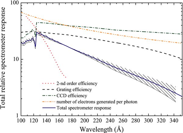
Figure 2. Overall relative spectrometer photon efficiency (%) curves as a function of the photon energy (wavelength, Å). The contributions of grating, CCD detector, second-order diffraction and the total efficiency are shown.
Download figure:
Standard image High-resolution image3.3. EUV Spectra of Highly Charged Fe Ions
In the following, 26 Fe spectra with very small pixel shifts (dx in Equation (1)) were analyzed in detail. The strong, isolated resonance lines at 284.164 Å (NIST value) due to the 2p63s3p1P1–2p63s2 1S0 transition of Fe xv and at 171.073 Å due to the 3s23p53d1P1–3s23p6 1S0 transition of Fe ix were used to monitor the pixel shift. Using the mean parameters (A, B, C, and D) given above and the estimated shift, the wavelength scales for an individual spectrum were determined. Once the wavelength scale was fixed with this procedure, nearly 200 emission lines were found and fitted locally using Gaussian profiles. One of these spectra taken under the electron beam of Ee = 5.64 keV/Ie = 320 mA is shown in Figure 3.

Figure 3. Comparison (107–353 Å) between the observed (corrected for total spectrometer response in Figure 2) (thick black step curve) and simulated total spectra summed over all the ions in different charge states (Fe vii–Fe xxiv, at mono-energetic electrons with Ee = 5.64 keV/Ie = 320 mA and an electron density of ne = 1.0 × 1012 cm−3). For clarity, the theoretical spectra for each ion are shift downward by 50 counts. Some dominant emission lines are labeled out. The second-order diffraction spectra in wavelength range of 200–353 Å is shown by a step curve (dark-red in (a)–(c). Some strong second-order and third-order diffraction lines are marked with (2) and (3), respectively. Several contamination from highly charge C and O ions are labeled too. The red arrows at top in each panel indicate that those lines are used for normalization of the simulated spectra for each ionic state.
Download figure:
Standard image High-resolution image3.4. Simulation and Line Identification and of Extreme-ultraviolet Spectra
To reproduce the observed spectra including the relative line intensities and to identify the emitted lines, a series of the collisional-radiative simulations was carried out. Here we assume that the electronic impact excitation and de-excitation, as well as the radiative decay rates among levels of each ion (see Table 1) are the main mechanism for level population. The population of excited levels from ionization and recombination processes is assumed to be small in comparison with those due to the direct electronic excitation and the following cascades. The population of a particular level is determined by solving a system of coupled rate equations given by
where Nqj is the population density of state j of ions with charge of q, ne is the electron density and Ci→j is the excitation/de-excitation rate from the state i to j. Aj→i is the spontaneous decay (transition) rate from j to i. The first term on the right-hand side represents the excitation to the state j from lower excited state, the first part of the second term represents the de-excitation into j from higher excited states and the second part represents the spontaneous decay to j, and the third term represents the de-excitation and its spontaneous decay to lower excited state from j, respectively. Using the data from FAC (Gu 2008) and quasi-stationary approximation for excited level (dNqj/dt = 0) for each Fe ionic state ranging from Fe vii to Fe xxiv, we obtain the level population and, furthermore, calculate the line intensity defined as
The calculated energies for ions of the present interest have been found to be in agreement with experimental values, which are available from the NIST version 3.0 (see footnote 6), within 1%. The corresponding theoretical wavelengths were corrected with these available experimental data. The detailed assessment of the atomic data will not be discussed here as it exceeds the scope of the present work. The atomic data of Fe vii–Fe xv have been used to analyze the EUV spectra from EBIT at low electron impact energies (Liang et al. 2009). The resultant line intensities (NqiAij where Nqi indicates the level population of the ith energy level of an ion in the charge state q and Aij refers to the decay rate of the i → j transition) are then convolved with a Gaussian profile with a line width of 0.6 Å. Then, the simulated spectra at Ee = 5.64 keV and Ie = 320 mA with ne = 1.0 × 1012 cm−3 is normalized by the measured spectra by a single known emission line of each ionic state (see top arrows in each panel of Figure 3). The sum spectrum (blue solid curve) is the addition of all the theoretical spectra over Fe vii–Fe xxiv ions without higher order diffraction spectra. By using the second-order efficiency in Figure 2, we deduce the second-order diffraction spectra in wavelength range of 200–353 Å (see dark-red step curve in Figure 3).
Table 1. List of Configurations and Numbers of Levels (No. L) Included in the Present Simulation
| Ions | Configurations | No.L |
|---|---|---|
| Fe vii | [1s22s22p6]3s23p63d2, 3s23p53d3, 3s23p63d4l, 3s23p63d5l, 3s3p63d3, | 1891 |
| 3s23p53d24s, 3s23p64s2, 3s23p64s4p, 3s23p64s4d, 3s23p64p2, | ||
| 3s23p64p4d, 3s23p43d4, 3s23p33d5, and 3s3p53d4 (l = s, p, d, f, and g) | ||
| Fe viii | [1s22s22p63s2]3p63d, 3p53d4s, 3p53d4p, 3p64l, 3p65l (l = s, p, d, and f) | 149 |
| Fe ix | [1s22s22p6]3s23p6, 3s23p53d, 3s3p63d, 3s23p43d2, and 3s23p54l (l = s, p, and d) | 154 |
| Fe x | [1s22s22p6]3s23p5, 3s3p6, 3s23p43d, 3s3p53d, 3s23p44l, 3s3p54s, | 172 |
| 3s3p54p, 3s23p45s, 3s23p55p, and 3s3p55s (l = s, p, and d) | ||
| Fe xi | [1s22s22p6]3s23p4, 3s3p5, 3s23p33d, 3s23p34l, 3s23p35s, and 3s23p35p (l = s, p, and d) | 161 |
| Fe xii | [1s22s22p6]3s23p3, 3s3p4, 3p5, 3s23p23d, 3s3p3d2, 3s3p33d, and 3s23p24l (l = s, p, and d) | 160 |
| Fe xiii | [1s22s22p6]3s23p2, 3s3p3, 3p4, 3s23p3d, 3s3p23d, 3s23d2, 3s23p4l, | 309 |
| and 3s3p24l (l = s, p, d, and f) | ||
| Fe xiv | [1s22s22p6]3s23p, 3s3p2, 3p3, 3s23d, 3s3p3d, 3s3d2, 3s24l, and 3s3p4l (l = s, p, d, and f) | 135 |
| Fe xv | [1s22s22p6]3l3l', 2p53s23d, 2p63l4l'', and 2p63l5l'' (l, l' and l'' = s, p, d, f, and g) | 295 |
| Fe xvi | [1s22s2]2p6[3l, 4l, 5l, 6l], 2p53s3l, 2p53p3d, and 2p53p2 (l = s, p, d, f, g, and h) | 161 |
| Fe xvii | [1s2]2s2p6, 2s22p53l, 2s22p43l3l', 2s2p63l, 2s22p54l, and 2s2p64l (l and l' = s, p, d, and f) | 512 |
| Fe xviii | [1s2]2s2p5, 2s2p6, 2s22p43l, 2s2p53l, 2p63l, 2s22p44l, 2s2p54l, 2s22p45l, | 396 |
| and 2p64l (l = s, p, d, and f) | ||
| Fe xix | [1s2]2s22p4, 2s2p5, 2p6, 2s22p33l, 2s2p43l, 2p53l, 2s22p34l, 2s2p44l, 2s22p35l, | 710 |
| and 2p54l (l = s, p, d, f, and g) | ||
| Fe xx | [1s2]2s22p3, 2s2p4, 2p5, 2s22p23l, 2s2p33l, 2p43l, 2s22p24l, 2s2p34l, 2s22p25l, | 785 |
| and 2s44l (l = s, p, d, f, and g) | ||
| Fe xxi | [1s2]2s22p2, 2s2p3, 2p4, 2s22p3l, 2s2p23l, 2p33l, 2s22p4l, 2s2p24l, 2s22p5l, | 614 |
| and 2p34l (l = s, p, d, f, and g) | ||
| Fe xxii | [1s2]2s22p, 2s2p2, 2p3, 2s23l, 2s2p3l, 2p23l, 2s24l, 2s2p4l, 2s2p5l, 2s25l, 2p24l, | 513 |
| and 2p25l (l = s, p, d, f, and g) | ||
| Fe xxiii | [1s2]2s2, 2s2p, 2p2, 2s3l, 2p3l, 2s4l, 2p4l, 2s5l, and 2p5l (l = s, p, d, f, and g) | 166 |
| Fe xxiv | 1s22s, 1s22p, 1s23l, 1s24l, 1s24l, 1s25l, 1s26l, 1s2s2p, and 1s2p2, 2p3 (l = s, p, d, f, g, and h) | 55 |
Download table as: ASCIITypeset image
Figure 3 demonstrates that the present simulations satisfactorily reproduce the measured spectra. This supports the following discussions on the effective electron density and electron–ion cloud overlapping. For some emission lines at longer wavelengths (>220 Å), significant deviations were observed and found to be caused by the second-order diffraction (see marks with (2) in Figure 3(b)). Based upon the present simulated spectra and the recorded emission lines between 90 and 120 Å, we further note several third-order diffraction lines (see marks with (3) in Figure 3). Several contaminations from highly charged C v, O iv, and O v ions have been identified with the aid of the NIST list (see footnote 6).
3.5. Polarization Effect
The nonthermal unidirectional electrons in the present EBIT experiment will result in an anisotropy of emitted line radiations (Gu et al. 1999; Savin et al. 1996; Zhang et al. 1990; Shlyaptseva et al. 1998). This anisotropy results from the unidirectionality of the electron beam which can cause a population imbalance of the magnetic sublevels (m(−J)) and(m(+J)) leading to a possible linear polarization of the EUV emission. The observed line intensity, I(90°) (emitted at 90° to the electron beam direction), has a relation to the total emitted line intensity I in 4π steradians as follows:
where P is the polarization of the transition of interest.
Using the FAC, electron impact collision strengths among the magnetic sublevels of Fe vii–Fe xxiv ions have been calculated. By solving the extended rate equation (see Equation (1) in the work of Liang et al. (2009)), we obtain the magnetic sublevel population, and further the polarization P.
In Figure 4, we compare the synthetic spectra for monoenergetic electrons (Ee = 5.64 keV with ne = 1.0 × 1012 cm−3) with and without polarization effect for Fe xxi and Fe xi–Fe xiv ions. The polarization reduces some observed line intensities, e.g., the 2s2p3 3D1 → 2s22p2 3P0 transition of Fe xxi at 128.755 Å by 13%; the 3s23d2D5/2→3s23p2P3/2 of Fe xiv at 219.130 Å by 24%, where P < 0. We also note some observed line intensities are enhanced when the polarization effect (P > 0) is included, e.g., the 3s3p2 2P3/2 → 3s23p2P3/2 transition line of Fe xiv at 264.790 Å by 20%. This reveals that the polarization plays an important role on the observed line intensity for some emission lines at high electron energies. Therefore, we should be cautious when determining the line intensity ratios and the corresponding effective electron density (neffe) of the EBIT plasma using the EUV line ratio technique.
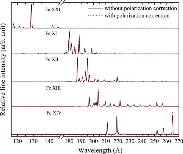
Figure 4. Comparison of the synthetic spectra of Fe xi–Fe xiv and Fe xxi ions without (blue) and with (red) polarization correction at Ee = 5.64 keV and ne = 1.0 × 1012 cm−3.
Download figure:
Standard image High-resolution image4. ION CHARGE STATE DISTRIBUTIONS
EUV spectroscopy has been extensively used to determine the radiation transfer as well as the ionization balance in various plasmas, as mentioned above. By analyzing the measured EUV emission line intensities, corrected for the spectrometer response, from ions in different charge states, it is possible to extract information on the charge state distributions (CSD) of the trapped ions using the known electron excitation cross sections derived from the empirical formula of Van Regemorter (1962) and the branching ratios. A series of well-resolved emission lines of Fe vii–Fe xxiv recorded in the present EBIT experiment (see Figure 3) was used to derive the CSD.
Since the electron beam energy of 4.5–5.64 keV used in the present experiment is much higher than the ionization potential of Li-like Fe23+ ions (2.05 keV), He-like Fe24+ ions can also be produced. However, none of their corresponding strong emission lines are present and indeed recorded on the spectrometer in the present measurement. No emission lines projected close to the edges of CCD were used. An additional 10% error to the inferred charge fractions was included to account for the systematic errors in the spectrometer spectral sensitivity (see Figure 2).
Figure 5 shows the relative CSDs of Fe ions in the trap produced with the electron beam having slightly different EBIT parameters: 4.5 keV/197 mA, 5.0 keV/400 mA, and 5.64 keV/320 mA. Though no information was obtained for He-like Fe24+ ions, the dominant ion charge state was found to be q = 23 (Li-like) Fe23+ with about 27% among the observed total ion fractions in the present experiment. A tail toward low charge states is observed, indicating that the continuous gas injection into the trap may replenish ions in lower charge states and also that the electron capture with the injected and residual neutrals tends to decrease the average ion charge states. The CSDs did not change significantly and also no systematic variations have been found among the present measurements under only slightly different EBIT electron beam parameters.

Figure 5. CSD of Fe ions produced at the EBIT with slightly different electron energies, currents, and neutral gas pressures. The data points with error bars show the spectroscopically extracted CSD. The histograms indicate the simulated charge distributions with an electron beam of 5.64 keV/320 mA at different gas pressures.
Download figure:
Standard image High-resolution imageA simulation of the CSD in the EBIT (Liu et al. 2005) was performed at different trap pressures (see Figure 5). By increasing the trap pressure (from 2.5 to 9.8 × 10⁻⁹ mbar), the maximum intensity ion charge in CSD gradually shifts from Fe23+ to Fe21+ with an increasing tailing toward lower charge states, meanwhile, the ion fractions at higher charge states (Fe23+–Fe24+) decrease significantly. Such tendencies are well understood due to the electron capture between the HCI and neutral gas atoms in the trap region. Note that, in the present experiment, relatively high injection pressures were used.
As no fraction of He-like Fe24+ ions could be determined as their emission lines are outside the spectral range under the present observation, it is hard to get a convincing conclusion from direct comparison with the simulated population distributions of these ions. Yet, it can be concluded that the CSDs in both observation and simulation show general agreement in their trends, except for He-like Fe24+ ions.
5. E FFECTIVE ELECTRON DENSITIES AND ELECTRON-ION OVERLAP
5.1. Electron Density Estimated Through EUV Spectroscopy
The observed line intensities of ions in various charge states provide information on their population distribution (see Section 4) and the plasma parameters in the trap. In particular, the electron density, a critically important parameter in all kinds of plasmas, can be determined with the help of EUV spectroscopy. In the EBIT, the electron density depends on a number of its running parameters such as the electron energy and current, the magnetic field strength, the vacuum, the trapping conditions, etc.
The allowed EUV transitions follow excitation so quickly (in a matter of ps) that the light emission pattern basically reflects the ion–electron beam overlap region (re) in which the excitation actually takes place. On the other hand, ions emitting photons through the decay of long-lived metastable electronic states can leave the electron beam region before the radiative transition occurs. The actual radius (ri) of ion cloud in the EBIT can be, under certain conditions, larger than the electron beam radius re, as the artist's representation shown in Figure 6. A real physical simulation of an ion orbit in EBITs is given in the work of (Gillaspy et al. 1995, see Figure 2). Then, the effective electron density (neffe) depends on the geometric overlap ( for
for  ) between the spatial distributions of the monoenergetic electron beam and those of the ion cloud in the trap region. Indeed, the effective electron density (neffe) governs basically the actual rates of all excitation and ionization processes in the EBIT.
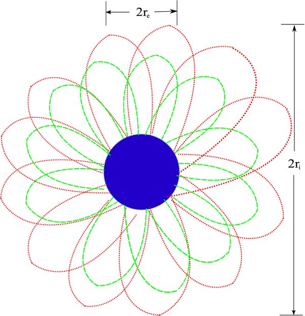
Figure 6. Schematic representation of the overlap of electron beam and ion cloud in the trap. re and ri represent the radius of electron beam (dark blue circle) and of ion cloud (trajectories), respectively. If ions in some electronically excited states populated in electron collisions have long lifetimes, they may decay outside the overlap region after excitation. Notes: this is an artist's representation, a real physical simulation is given in the work of Gillaspy et al. (1995).
Download figure:
Standard image High-resolution imageThe geometrically averaged electron density (nge) can be estimated from the electron beam size:
where e, Ie, re, and ve are the electronic charge, the electron beam current, radius, and velocity, respectively. We estimate the geometrical electron density nge of 1.6 × 1013 cm−3 under the present conditions (Ee = 5.64 keV, Ie = 320 mA, re = 30 μm).
However, we have no information on the spatial distributions of ions in the present experiment and only those forbidden lines can give a true representation of the ion spatial distributions, since the long elapsing time between excitation and radiative decay essentially decouples the light emission spatial pattern from the geometry of the narrow excitation region defined by the electron beam. Then, we have to infer the effective electron density neffe by a suitable spectroscopic diagnostic method, and then derive information on the ion–electron beam overlap factor for each charge state.
5.1.1. Fe xxi Ion Lines
The diagnostic potential of EUV lines from Fe ions for determining neffe had been pointed out previously. The intensity ratios of several partner lines of the carbon-like Fe xxi ion are known to be sensitive to the electron density but rather insensitive to the electron temperature (Ness et al. 2004). This feature follows from the fact that the upper level is populated mainly through collisional excitation from a density-sensitive lower metastable level. As shown in Figure 7, the 2s2p3 3D2 level of this ion has a high excitation rate from and decay rate to the metastable 2s22p2 3P1 level, which is forbidden to decay to the ground state. By increasing the electron density, a significant fraction of the 3P1 population can be re-excited to the 3D2 state, which relaxes to the 3P1 state and, therefore, the line intensity at 142.148 Å increases. On the other hand, through depopulation of the ground state 3P0 due to the shelving of electrons into the metastable level (if production of the 3P0 level of Fe xxi from lower charge states is too slow), the excitation to the 3D1 state and therefore the first resonance line (3D1–3P0) intensity at 128.755 Å decreases at high electron densities, as illustrated in Figure 8(a).

Figure 7. Scheme of the processes responsible for the electron density-sensitive lines of the n = 2 → n = 2 transitions in Fe xxi. Only the lowest levels belonging to 2s22p2 and 2s2p3 configurations are depicted. Wavelengths (in Å) and radiative branching ratios different from 100% are indicated (dashed lines). Relative magnitudes of collisional excitation strengths at Ee = 5.64 keV are given in percentage as well as represented by the thickness of the corresponding solid lines.
Download figure:
Standard image High-resolution image
Figure 8. (a) Relative line intensities (without polarization effect) of three interest Fe xxi lines as a function of the electron density for mono-energetic electrons at 5.64 keV (solid lines) and thermal electrons (at Te = 1.0 × 10⁷ K, dashed lines) (b) Line intensity ratio,  of Fe xxi as a function of the electron density for monoenergetic electron beams (at 4.5, 5.0, and 5.64 keV) and for thermal electrons at Te = 1.0 × 10⁷ K. Symbols with error bars are the measured line ratios. The hatch areas show predictions for thermal electrons in the temperature range of 5.0 × 10⁶–5.0 × 10⁷ K. The expanded inset clearly shows the line intensity ratios with polarization effect.
Download figure:
Standard image High-resolution imageIt is important to note that the 2s2p3 3D1 state can also decay to the metastable 3P1 state with a low branching ratio. As this transition line (at 142.278 Å) cannot be resolved from the 142.148 Å line due to the limited spectrometer resolution, we have to take this blending effect into account. Since the 2s2p3 3D1 level is directly populated from the ground state, the intensity of 142.278 Å line has a dependence on ne which is similar to that of the 128.755 Å resonance line, and its relative contribution to the total line intensity becomes dominant below the electron density of ne = 1.0 × 1012 cm−3. On the other hand, at higher electron densities, the 142.148 Å line becomes more intense. As shown in Figure 8(a), the line intensities, I(142.148 Å), I(142.278 Å), and I(128.755 Å), are calculated for a plasma excited by monoenergetic electrons (Ee = 5.64 keV) and also for thermal electrons (Te = 1.0 × 10⁷ K) as a function of the electron density. These results indicate that the intensity of 142.148 Å line is greatly affected by the electron energy distributions (see the dashed red line in Figure 8(a)). The monoenergetic electron beam populates predominantly the high-lying levels (3D1), whereas thermal energy electrons preferentially feed states with lower excitation energies. These effects result in a difference of the line intensity ratio in the two cases as shown in Figure 8(b). With increasing electron density, the deviations get weaker.
By applying the collisional-radiative model described above, we calculated the intensities of the lines of interest for different electron densities for both monoenergetic and thermal electrons. Figure 8(b) demonstrates the intensity ratios of  as a function of the electron density for both cases. The line intensity ratios for monoenergetic electron beam are depicted with three separate lines (blue: 4.5 keV, red: 5.0 keV, and black: 5.64 keV). The hatched bands (gray) indicate the ratio obtained for thermal electrons with the temperatures ranging from 5.0 × 10⁶ to 5.0 × 10⁷ K, showing that the line ratio is not too sensitive to the electron temperature. A noticeable difference of this ratio can be seen between monoenergetic and thermal electrons below the electron density of 3.0 × 1012 cm−3. This different behavior between two modes of excitation is due to the fact that the population of the 2s22p2 3P1 level, a major excitation channel to the upper 3D2 level which emits the 142.148 Å line, is greatly influenced by the electron energy distributions, as shown in Figure 8(a), resulting from features of electron collision processes that the excitation efficiencies of low energy electrons are higher than those of high energy electrons.
By comparing the calculated line intensity ratio  with the present experimental result (0.15 ± 0.01 at 5.64 keV/320 mA, the error in line intensities results from a quadrature sum of the errors from fitting the line shapes and spectrometer response uncertainty shown in Figure 2), the effective electron density was determined to be neffe = 2.60+0.4−0.39 × 1012 cm−3. At slightly different electron beam conditions (taken on different occasions), namely 5.0 keV/400 mA and 4.5 keV/197 mA, we have obtained 2.30 ± 0.42 × 1012 cm−3 and 7.8+4.0−3.9 × 1011 cm−3, respectively. The relatively large uncertainties are mainly due to the fact that the observed ratios are already close to the lower density limit (∼1011 cm−3). When the polarization effect is taken into account, the effective electron densities are estimated to 1.40+0.35−0.32 × 1012 cm−3 (5.64 keV/320 mA), 1.12+0.37−0.34 × 1012 cm−3 (5.00 keV/400 mA), and an upper limit 1.9 × 1011 cm−3 (4.50 keV/197 mA), respectively, indicating that exact information on the polarization is important.
5.1.2. Fe x Ion Lines
We have tried to check our EUV spectroscopy technique for estimating the electron densities using a different ion charge, namely Fe x ions, produced simultaneously under the same EBIT conditions. The upper level (3s23p43d2D5/2) of resonance transition line at 174.526 Å are populated dominantly by direct excitations from the ground state (3s23p5 2P3/2), as shown in Figure 9(a). The population of the excited level 2D3/2 is dominantly populated by excitation from the metastable level (2P1/2, 51%). So the line intensity of the transition (3s23p43d2D3/2 → 3s23p5 2P1/2, with a wavelength of 175.265 Å) is sensitive to the electron density. The upper level (2P1/2) of the transition line at 175.475 Å is also dominantly populated by excitation from the metastable level (25%). Its intensity (relative to that of the resonance line at 174.526 Å) is also sensitive to the electron density. In the present measurement, this transition line cannot be resolved from the line at 175.265 Å. By taking this blending effect into account, we calculate the line intensity ratio  of Fe x as a function of the electron density for monoenergetic electron beam (see Figure 9(b)).
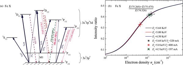
Figure 9. (a) Scheme of the processes responsible for the electron density-sensitive lines of the n = 3 → n = 3 transitions in Fe x. Only the levels of 3s23p5 and 3s23p43d configurations involved in the transitions of interest are depicted. Wavelengths (in Å) and radiative branching ratios different from 100% are indicated (dashed lines). Relative magnitudes of collisional excitation strengths at Ee = 5.64 keV are given in percentage as well as represented by the thickness of the corresponding solid lines. (b) Line intensity ratio, , of Fe x as a function of the electron density for monoenergetic electron beam (at 4.5, 5.0, and 5.64 keV). Symbols with error bars are the measured line ratios.
Download figure:
Standard image High-resolution imageBased upon this curve and from the present observed ratios, we have determined the effective electron densities to be 1.3+0.5−0.3 × 10¹¹, 4.6+1.0−0.8 × 10¹⁰, and 1.5+0.7−0.4 × 1011 cm−3 under 4.5 keV/197 mA, 5.0 keV/400 mA, and 5.64 keV/320 mA electron beams, respectively. Polarization effect on this line ratio is found to be negligible. Note that the errors are much smaller than those in Fe xxi because the observed ratios in Fe x ions are in the most density-sensitive region, compared with those in Fe xxi (see Figure 8).
5.1.3. Other Ion Lines
Other EUV line intensity ratios have been used to determine the electron density in solar corona, EBIT plasma, etc. (Keenan et al. 2005b—Fe xi; Del Zanna & Mason 2005—Fe xii; Yamamoto et al. 2008; Watanabe et al. 2009—Fe xiii). Here, we selected ne-sensitive lines without blending from emission lines of other ionic states to further estimate the electron density in the EBIT plasma under the electron beam energy and current of Ee = 5.64 keV and Ie = 320 mA, respectively. For example, the line intensity ratios (see Figure 10) with nearby wavelengths of Fe xi:  , Fe xii:
  , Fe xiii:
  , Fe xiv:
  , Fe xxii:
  . The corresponding transitions are listed in Table 2. The resultant effective electron densities are listed in Table 3. Note that the polarization correction is critical in some cases. We note that there is significant difference in the electron densities estimated from different ions under the completely same EBIT running conditions. It seems that there is a trend that higher effective electron densities are obtained from higher ionic charge under the same operation conditions. However, the result from Fe xiii slightly deviates from the trend.
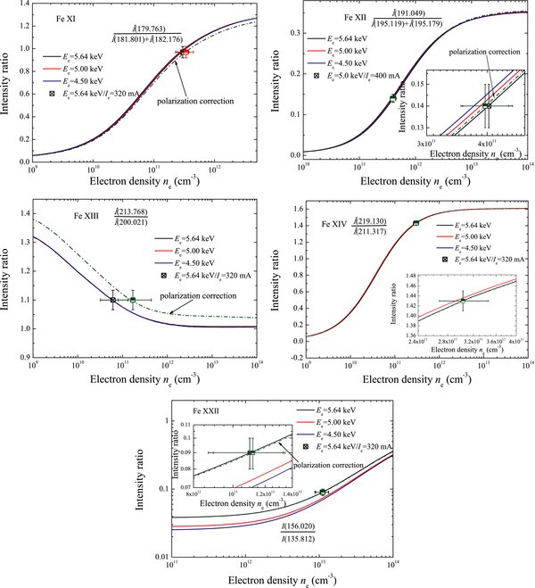
Figure 10. Line intensity ratios of Fe xi, Fe xii, Fe xiii, Fe xiv, and Fe xxii as a function of the electron density for monoenergetic electron beam at 4.5, 5.0, and 5.64 keV. Symbols with error bars are the measured line intensity ratios at 5.64 keV/320 mA. Green dash-dotted lines and marks represent ratios corrected for polarization.
Download figure:
Standard image High-resolution imageTable 2. Transition Lines Used in Estimation of the Effective Electron Density neffe
| λ(Å) | Transition | Ion | |
|---|---|---|---|
| 174.526 | 3s23p43d2D5/2 | →3s23p5 2P3/2 | Fe x |
| 175.265 | 3s23p43d2D3/2 | →3s23p5 2P1/2 | Fe x |
| 175.475 | 3s23p43d2P3/2 | →3s23p5 2P1/2 | Fe x |
| 179.763 | 3s23p33d1F3 | →3s23p4 1D2 | Fe xi |
| 181.801 | 3s23p33d3P0 | →3s23p4 3P1 | Fe xi |
| 182.176 | 3s23p33d3D2 | →3s23p4 3P1 | Fe xi |
| 191.049 | 3s23p23d2D5/2 | →3s23p3 2P3/2 | Fe xii |
| 195.119 | 3s23p23d4P5/2 | →3s23p3 4S3/2 | Fe xii |
| 195.179 | 3s23p23d2D3/2 | →3s23p3 2D3/2 | Fe xii |
| 213.768 | 3s23p3d3P2 | →3s23p2 3P3 | Fe xiii |
| 200.021 | 3s23p3d3D2 | →3s23p2 3P1 | Fe xiii |
| 264.789 | 3s3p2 2P3/2 | →3s23p2P3/2 | Fe xiv |
| 274.203 | 3s3p2 2S1/2 | →3s23p2P1/2 | Fe xiv |
| 128.755 | 2s2p3 3D1 | →2s22p2 3P0 | Fe xxi |
| 142.148 | 2s2p3 3D2 | →2s22p2 3P1 | Fe xxi |
| 142.278 | 2s2p3 3D1 | →2s22p2 3P1 | Fe xxi |
| 135.812 | 2s2p2 2D3/2 | →2s22p2P1/2 | Fe xxii |
| 156.020 | 2s2p2 2D5/2 | →2s22p2P3/2 | Fe xxii |
Download table as: ASCIITypeset image
Table 3. Effective Electron Densities (cm−3) for Iron Ions With Different Charges in the EBIT Plasma
| Effective Electron Density | ||
|---|---|---|
| Ion | neffe | neffe(Correction for Polarization) |
| Fe x | 1.5+0.7−0.4 × 10¹¹ | 1.5+0.7−0.4 × 10¹¹ |
| Fe xi | 3.0+0.8−0.7 × 10¹¹ | 3.4+1.1−0.9 × 10¹¹ |
| Fe xii | 4.03+0.48−0.47 × 10¹¹ | 3.98+0.47−0.43 × 10¹¹ |
| Fe xiii | 6.1+0.7−0.3 × 10¹⁰ | 1.7+0.3−0.9 × 10¹¹ |
| Fe xiv | 3.03+0.43−0.35 × 10¹¹ | 3.03+0.43−0.35 × 10¹¹ |
| Fe xxi | 2.60+0.40−0.39 × 10¹² | 1.4+0.35−0.32 × 10¹² |
| Fe xxii | 1.10+0.23−0.23 × 10¹³ | 1.12+0.22−0.23 × 10¹³ |
Note. Effective electron densities (cm−3) for iron ions with different charges in the EBIT plasma under Ee = 5.64 keV/Ie = 320 mA, estimated from line intensity ratios without and with polarization corrections (see Figures 8–10) of Fe x–Fe xxii.
Download table as: ASCIITypeset image
Watanabe et al. (2009) performed the electron density diagnostic for the solar active region with Fe xiii line ratios and Hinode8 EUV imaging spectrometer (EIS) spectra, in which many line ratios were presented (see Figure 3 in their work). However, most emission lines of Fe xiii are blended by lines of other ionic charge states in our present measurement. In this work, we try to use ratios of lines without contamination. So the two contamination-free density-sensitive lines are used here (see Figures 3 and 11), which differs from other cases, e.g., Fe x and Fe xxi, one resonance line and one density-sensitive line (the population of the upper level is dominated by excitations of the metastable level). Due to the different competitions for level population, the line intensity ratio between them also shows a good sensitivity to the electron density. As explored by Watanabe et al. (2009), different models show a slight discrepancy using different atomic parameters. Generally, the atomic parameters for forbidden transitions (decays from metastable levels) show a larger uncertainty than those for resonance transitions. Hence, the ratio between two density-sensitive lines shows a slightly larger deviation than other ratios between the density-sensitive line and the resonance line.

Figure 11. Scheme of the processes responsible for the electron density-sensitive lines of the n = 3→n = 3 transitions in Fe xiii. Only the levels of 3s23p2, 3s3p3, and 3s23p3d configurations involved in the transitions of interest are depicted. Wavelengths (in Å) and radiative branching ratios different from 100% are indicated (dashed lines). Relative magnitudes (>1%) of collisional excitation strengths at Ee = 5.64 keV are given in percentage as well as represented by the thickness of the corresponding solid lines.
Download figure:
Standard image High-resolution image5.2. Ion Cloud Sizes and Electron–Ion Beam Overlap
At first glance, it is quite surprising that the effective electron densities neffe observed from the transition lines are so small (less than 2 orders of magnitude), compared with simple geometrical electron densities nge (see Equation (5)) and also much different between differently charged ions observed under the same EBIT conditions. In order to understand such features, it is interesting to compare the observed "effective" electron densities neffe with the "geometrical" electron densities nge calculated from Equation (5). These results are summarized in Table 4 demonstrating that the neffe/nge ratios vary by almost 2 orders of magnitude. Low charged ions show low ratios and higher charged ions show higher ratios.
Table 4. Estimated Electron Density Ratios (neffe/nge) and Ion Radius Ratios (ri/re)
| Electron Density Ratio (neffe/nge) | ||||
|---|---|---|---|---|
| Ion | 4.5 keV/197 mA | 5.0 keV/400 mA | 5.64 keV/320 mA | ri/re |
| Fe x | 1.2+0.5−0.3 × 10⁻² | 9.4+4.4−2.5 × 10⁻³ | 8.5–12.0 | |
| Fe xi | 1.8+0.4−0.3 × 10⁻² | 2.1+0.7−0.6 × 10⁻² | 5.9–8.0 | |
| Fe xii | 2.5+0.3−0.3 × 10⁻² | 6.0–6.7 | ||
| Fe xiii | 1.1+0.2−0.6 × 10⁻² | 8.9–14 | ||
| Fe xiv | 1.6+0.4−0.3 × 10⁻² | 1.9+0.3−0.2 × 10⁻² | 6.8–7.8 | |
| Fe xxi | <1.7 × 10⁻² | 5.3+1.8−1.6 × 10⁻² | 8.8+2.2−2.0 × 10⁻² | 3.0–3.8 |
| Fe xxii | 6.8+2.6−2.2 × 10⁻¹ | 7.0+1.4−1.4 × 10⁻¹ | 1.1–1.4 | |
Note. Estimated electron density ratios (neffe/nge) and ion radius ratios (ri/re) from highly charged iron ions taken under slightly different EBIT conditions.
Download table as: ASCIITypeset image
Similar observations of the effective electron densities under quite different electron beam conditions (1–3 keV and 1–10 mA) in an EBIT at Livermore were performed based upon soft X-ray spectroscopy of helium-like N vi ions (Chen et al. 2004). Silver et al. (2000) and Matranga et al. (2003) also performed similar diagnostic of the electron densities for the NIST EBIT plasmas using K-shell X-ray spectroscopy. The lifetimes of the levels observed are much shorter than the present metastable levels of Fe ions. A linear behavior between the electron densities and [Ie/E1/2e] was indeed suggested under a fixed electron beam radius by Chen et al. (2004) (see Figure 6 in their work) based upon their limited experimental data. Considering that most of EBITs all over the world have similar (designed) electron beam radii, we combined the data available so far into our present analysis as shown in Figure 12. The relative normalized electron density neffe/[Ie/E1/2e] clearly deviates from such expectation. Particularly such deviations at high [Ie/E1/2e] values with high electron current (like in the present work) region are significant, compared with those at low [Ie/E1/2e] values (like in Livermore experiment by Chen et al. 2004). This trend can be understood: at high electron currents, the ions tend to be more heated and thus their radii get large, resulting in a lower effective electron density. As the effective electron density depends on the overlap between ion cloud and electron beam, the deviation observed indicates a significant change of the ion–electron beam overlap f which depends on [Ie/E1/2e], and also the axial trap voltage applied on the end cap drift tubes on both sides of the central drift tube as explored by Porto et al. (2000). The significant deviations for lower charged iron ions in the present results mean a smaller overlap than previously found at high electron energy/high current results. By taking the polarization effect into account, we re-analyze our previous measurements with low energies and currents (Ee = 70–500 eV and Ie = 2.1–8.0 mA) at the Heidelberg FLASH-EBIT (Liang et al. 2009). Significant deviation appears again as illustrated by dark-green square symbols in Figure 12, indicating a smaller overlap for the lower charged ions. The large scattering in the present results is due to the overlap f (or r2i/r2e) dependence on the ionic charge as will be explained in the following.
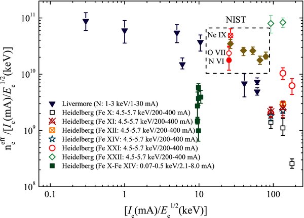
Figure 12. Comparison of "relative" normalized effective electron density (cm−1) among various EBIT experiments. The data of Livermore (blue triangles) are taken from the work of Chen et al. (2004); NIST data within the rectangle with dash boundary are from Silver et al. (2000) (circles: N vi, O vii, and Ne ix) and Matranga et al. (2003) (diamonds: Ne ix); The data of Heidelberg at low energies and currents (0.07–0.5 keV/2.1–8.0 mA, dark-green filled square) are from our re-analyzing to the spectra of Liang et al. (2009) with polarization effect taken into account. The open symbols refer to the present results. Notes: the electron densities from literatures are normalized by the corresponding values of [Ie/E1/2e].
Download figure:
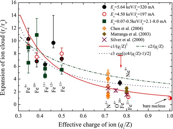
Standard image High-resolution imageThe ratios, ri/re, of the ion cloud radius over the electron beam radius obtained from the observed neffe/nge ratios are illustrated in the last column of Table 4. The range of ion radius ratio against the real electron radius thus estimated show that the ion clouds significantly expand far outside (∼10 times) the geometrical electron beam radius re for lower charged ions in the Heidelberg FLASH-EBIT, particularly for Fe x and Fe xiii (see Table 4 and Figure 13) in the present measurement. This large expansion of the ion could be understood due to the axial trap of 360 V applied on the end cap trap tubes. Porto et al. (2000) experimentally demonstrated that the width of ion cloud (Ar13+) would increase by a factor of ∼5 from an open trap to a deep trap with the static trapping voltage of 300 V (see Figure 6 in their work). However, for higher charged ions (Fe xxi and Fe xxii), the ion cloud was found to be less expanded. Thus, it is concluded that the expansion of ion clouds has a dependence on the ionic charge. Though the present data are limited, there is a clear trend that ions with higher charge (Fe20+ and Fe21+) have less expanded. Assuming the diameter of electron beam to be ∼60μm in the work of Silver et al. (2000), Matranga et al. (2003), and Liang et al. (2009), we further derive the ion expansion in their measurements. Though these measurements were performed with different trap conditions at different EBITs, a quantitative relation between the expansion of ion clouds and the effective charge of ions can be concluded. Figure 13 demonstrates that the expansion (ri/re) of iron ion cloud has a relation with the effective charge of ions 1/(qi/Z)α with 1 < α ⩽ 2. It is noted that the Levine's model (Levine et al. 1988) of the inverse exponential expansion of ion cloud size seems to be slightly off from the general trend including all the possible ion charge data available. At comparable values of the effective charge of ions, the expansion of Ne8+ ion cloud in works of Matranga et al. (2003) and Silver et al. (2000) shows a similar expansion as Fe21+ ion cloud extracted in the present measurement though they are generated at different EBITs with different conditions. Measurements by Silver et al. (2000) at slightly different conditions for N5+ and O6+ (2.0 keV/35.9 mA), as well as Ne8+ (2.2 keV/39.5 mA) also show such dependence on the effective ion charge. The data from Chen et al. (2004) demonstrate the dependence of the expansion of ion could (N5+) on the operation conditions of EBIT as revealed in Figure 12.
Figure 13. Expansion of ion cloud radius (ri) relative to the electron beam size (re) as a function of the effective charge of ion (qi/Z, Z is the nuclear charge of ion). The NIST data from Silver et al. (2000) (for N, O, and Ne ions) and Matranga et al. (2003) (for Ne ions), as well as Livermore data from Chen et al. (2004) (for N ions) were added by assuming re = 30 μm. The data point at qi/Z = 1.0 is not a "real" data, which is based upon the assumption that the bare nucleus should completely overlap with the electron beam. The three curves represent analytic relation between ri/re and the effective charge of ion (qi/Z), where c1, c2, c3, and c4 are constant values making the curves to fit the present measured data points.
Download figure:
Standard image High-resolution image
There are only very few direct observations on such large expanded ion clouds. NIST group has reported their results for ion cloud sizes in their EBIT by measuring lines from metastable state ions (Porto et al. 2000). Under their EBIT conditions, these ions have been found to spread out up to 400 μm radius, compared with their estimated electron radius (35 μm). Their results for Ar13+ ions provide some clues and support in understanding the present results. This is generally in agreement with a recent observation based upon visible photon spectroscopy at MPI. Another observation shows that the Ar13+ ion cloud radius is observed to reach 250 μm (Draganic 2007) under lower energy electrons. These measurements support our present estimations based upon the EUV spectroscopy.
In the following, we present an analytical representation for the dependence of the overlap f on the charge of ions for an EBIT plasma. We assume a radial Boltzmann distribution for the ion cloud of charge state qi

and a Gaussian shape for the electron beam density radial distribution
where re refers to the electron beam radius estimated by Herrmann's theorem (Herrmann 1958),  is the temperature of thermalized ions with charge of qi. The potential function ϕ(r) = ϕe(r) + ϕi(r) accounts for the space charge potential of the compressed electron beam and radial screening by ions, respectively. ϕe(r) is expressed as follows by Gillaspy (2001):
where rdt represents the radius of the central drift tube of the EBIT,  0 is permittivity and ve is the electron velocity. The ion charge density ni and the potential are connected by Poisson's equation, which can be solved numerically:
From Equations (6)–(10), we can see that the overlap factor  has a strong dependence on the ionic charge.
6. SUMMARY AND OUTLOOK
EUV spectra (107–353 Å) of highly charged Fe ions were observed under unidirectional electron beam with slightly different energies (4.5–5.64 keV) and currents (197–400 mA) by a flat-field grating spectrometer mounted at the Heidelberg FLASH-EBIT. The results obtained can be summarized as follows:
- 1.Collisional-radiative simulations under monoenergetic and thermal electrons were carried out, and the results obtained in the monoenergetic excitation case satisfactorily reproduced the observed EUV emission spectrum of highly charged Fe ions in the EBIT, helping line identification and disentanglement of satellite lines.
- 2.Comparison of the simulated spectra with and without polarization from unidirectional electron impact reveals that the polarization effect can either reduce or enhance some line intensities up to 24%.
- 3.Through analysis of the measured line intensities (corrected for the spectrometer efficiencies) among different ion charges under 5.64 keV/320 mA electron impact, it has been found that the resulting CSD peak at Fe23+ among the observed ions, though with the present EUV spectrometer we could not observe any lines from Fe24+, and tail toward lower charge states. A simulation also reproduces nicely this behavior, indicating that a shift to lower charge states with increasing injected gas pressure is due to electron capture into HCI from neutral atom.
- 4.Based upon the electron-density-sensitive EUV line intensity ratios of ions from Fe x to Fe xxii, the estimated effective electron densities of the EBIT plasmas under only slightly different electron beam conditions were found to be critically dependent on the ionic charge which we analyzed: the cloud of lower charged ions (e.g., Fe x) expand up to nearly 10 times beyond the electron beam radius, whereas those of higher charged ions expand less, and e.g. the Fe xxii ion cloud is close to the geometrical electron size (of 2re). For the first time, we have observed a significant difference of the ion–electron overlap strongly depending on the ion charge even under the same EBIT running conditions.
- 5.Combining the present results with those obtained in previous experiments for a wide range of the ions (N vi ∼ Ne ix) under very much different (a few hundred electron volt and a few milliampere electron beam) conditions, we have found a relatively simple scaling rule for estimating the ion cloud/electron beam size ratios as a function of the effective ion charge (q/Z).
In conclusion, the present EUV spectroscopic measurements have provided detailed insights into the ionization and excitation conditions of HCI confined in the EBIT, suggesting that the EBIT is a powerful, convenient laboratory plasma source which can provide crucial information on interpretation of the observations and diagnostics applicable to various plasma processes. The existing discrepancies between the present observations and simulations still demand more detailed studies on EBIT-produced plasmas. However, these are small despite of the fairly simple models used in the present simulations, compared to those typically used in the description of high temperature, low-density astrophysical plasmas. Furthermore, more detailed investigations of the ion–electron beam overlapping should be performed under various EBIT running conditions in order to get more exact insight in electron–ion interactions including the cross sections such as ionization and excitation obtained from the EBIT and the ionization time or charge balance of ions or more general simulations in the EBIT.
G.Y.L. acknowledges the help from the whole HD-EBIT-team. Funding is provided by MPI-K, and partially from support of National Science Foundation of China under grant Nos. 10603007 and 10821061 and National Basic Research Program of China (973 program) under grant No. 2007CB815103.
Footnotes
- 6
- 7
- 8