


ABSTRACT
We present the Spectroscopic Imaging survey in the near-infrared (near-IR) with SINFONI (SINS) of high-redshift galaxies. With 80 objects observed and 63 detected in at least one rest-frame optical nebular emission line, mainly Hα, SINS represents the largest survey of spatially resolved gas kinematics, morphologies, and physical properties of star-forming galaxies at z ∼ 1–3. We describe the selection of the targets, the observations, and the data reduction. We then focus on the "SINS Hα sample," consisting of 62 rest-UV/optically selected sources at 1.3 < z < 2.6 for which we targeted primarily the Hα and [N ii] emission lines. Only ≈30% of this sample had previous near-IR spectroscopic observations. The galaxies were drawn from various imaging surveys with different photometric criteria; as a whole, the SINS Hα sample covers a reasonable representation of massive M⋆ ≳ 1010 M☉star-forming galaxies at z ≈ 1.5–2.5, with some bias toward bluer systems compared to pure K-selected samples due to the requirement of secure optical redshift. The sample spans 2 orders of magnitude in stellar mass and in absolute and specific star formation rates, with median values ≈3 × 10¹⁰ M☉, ≈70 M☉ yr−1, and ≈3 Gyr−1. The ionized gas distribution and kinematics are spatially resolved on scales ranging from ≈1.5 kpc for adaptive optics assisted observations to typically ≈4–5 kpc for seeing-limited data. The Hα morphologies tend to be irregular and/or clumpy. About one-third of the SINS Hα sample galaxies are rotation-dominated yet turbulent disks, another one-third comprises compact and velocity dispersion-dominated objects, and the remaining galaxies are clear interacting/merging systems; the fraction of rotation-dominated systems increases among the more massive part of the sample. The Hα luminosities and equivalent widths suggest on average roughly twice higher dust attenuation toward the H ii regions relative to the bulk of the stars, and comparable current and past-averaged star formation rates.
Export citation and abstract BibTeX RIS
1. INTRODUCTION
In the now standard model of concordance cosmology, large-scale structure grows through simple gravitational aggregation and collapse from the initial fluctuations in the mass density of the early universe. In this framework, galaxies form as baryonic gas cools at the center of dark matter halos and subsequently grow through accretion and mergers, leading to the hierarchical buildup of galaxy mass. Increasingly deep and wide-area multiwavelength surveys in the past decade have established a fairly robust outline of the global evolution of galaxies over nearly 90% of the age of the universe. Rapid evolution is observed at redshifts z ∼ 1–4, with the peak of (dust-enshrouded) star formation, luminous QSOs, and major merger activity occurring around z ∼ 2–3 (e.g., Fan et al. 2001; Chapman et al. 2005; Hopkins & Beacom 2006). By z ∼ 1, roughly half of the stellar mass in galaxies—and >90% in massive, ≳1011 M☉ galaxies—was assembled (e.g., Dickinson et al. 2003; Fontana et al. 2003; Rudnick et al. 2003, 2006; Grazian et al. 2007; Conselice et al. 2007). The epochs around z ∼ 1–2 also seem to correspond to a crucial transition with the emergence of the bimodality and the Hubble sequence as observed in the present-day galaxy population (e.g., Bell et al. 2004; van den Bergh et al. 1996, 2001; Lilly et al. 1998; Stanford et al. 2004; Ravindranath et al. 2004; Papovich et al. 2005; Kriek et al. 2008a; Williams et al. 2009).
The details of how galaxies were assembled and evolved remain, however, poorly known. Much of our current knowledge at z ≳ 1 still relies heavily on galaxy-integrated spectral energy distributions (SEDs) and colors, and on global properties such as stellar mass and age, star formation rate (SFR), interstellar extinction, and sizes. Studies based on integrated spectroscopy (mostly in the optical, much fewer in the infrared and submillimeter) are still comparatively scarce but have provided secure redshifts for various photometrically selected samples, and first results notably on galactic-scale outflows, dynamical masses, gas mass fractions, and nebular abundances. More direct and detailed constraints are however needed to understand the formation and evolution of galaxies, involving angular momentum exchange and loss, cooling, dissipation, dynamical processes, and feedback from star formation and active galactic nuclei (AGNs). Such constraints are crucial as input and benchmarks for theories and simulations of galaxy formation and evolution.
Of particular relevance in this context is the issue of the dominant mechanisms by which massive galaxies at high redshift assemble their baryonic mass, and what processes drive their star formation activity and early evolution. While major merging is undoubtedly taking place at high redshift (e.g., Tacconi et al. 2006, 2008), new observational results suggest that rapid but more continuous gas accretion via "cold flows" and/or minor mergers likely played an important role in driving star formation and mass growth of the massive star-forming galaxy population at z ≳ 1 (e.g., Noeske et al. 2007; Elbaz et al. 2007; Daddi et al. 2007). This is in line with recent theoretical work based on both semianalytical approaches and hydrodynamical simulations (e.g., Kereš et al. 2005; Dekel & Birnboim 2006; Kitzbichler & White 2007; Naab et al. 2007; Guo & White 2008; Davé 2008; Genel et al. 2008; Dekel et al. 2009b). The results from our own SINFONI survey of kinematics of z ∼ 2 galaxies (the subject of the present paper), as well as similar studies carried out by other teams (e.g., Erb et al. 2003, 2006b; Law et al. 2007a, 2009; Wright et al. 2007, 2009) have provided key evidence in support of this alternative scenario, at least in a significant number of galaxies observed.
This emphasizes the crucial role of spatially and spectrally resolved investigations of individual galaxies at early stages of their evolution. Such studies enable the mapping of kinematics and morphologies, and of the distribution of star formation, gas and stars, and physical properties such as chemical abundances and excitation state of the gas. The constraints and results can then be fed into studies of larger samples (connecting through global galaxy parameters such as mass and SFR), and theoretical models and numerical simulations (as observationally motivated ingredients and assumptions). Obtaining spatially/spectrally resolved data is however notoriously challenging because of the faintness of high-redshift galaxies, and also because many important spectral diagnostic features are redshifted out of the optical bands. The advent of sensitive near-infrared (near-IR) integral field spectrometers mounted on 8–10 m class ground-based telescopes have recently opened up this avenue (e.g., Förster Schreiber et al. 2006a; Genzel et al. 2006; Nesvadba et al. 2006a, 2006b, 2007, 2008; Swinbank et al. 2006, 2007; Law et al. 2007a, 2009; Wright et al. 2007, 2009; Bournaud et al. 2008; van Starkenburg et al. 2008; Stark et al. 2008; Maiolino et al. 2008; Épinat et al. 2009). These new instruments provide simultaneously the two-dimensional (2D) spatial mapping and the spectrum over the entire field of view (FOV). Operating at near-IR wavelengths, they enable one to access, for z ∼ 1–4, well-calibrated spectral diagnostics of the physical properties from rest-frame optical emission lines such as Hα, Hβ, [N ii] λλ 6548, 6584, [O iii] λλ 4959, 5007, [O ii] λ 3727, and [S ii] λλ 6716, 6731.
Using the near-IR integral field spectrometer SINFONI (Eisenhauer et al. 2003a; Bonnet et al. 2004) at the Very Large Telescope (VLT) of the European Southern Observatory (ESO), we have carried out a major program of spatially resolved studies of high-redshift galaxy populations: the Spectroscopic Imaging survey in the near-IR with SINFONI, or "SINS." With the rich information provided by SINFONI on individual galaxies, the key science goals of the SINS survey are to investigate in detail (1) the nature and timescales of the processes driving baryonic mass accretion, star formation, and early dynamical evolution, (2) the connection between bulge and disk formation, (3) the amount and redistribution of mass and angular momentum within galaxies, and (4) the relative role and energetics of feedback from star formation and AGN.
Our initial results, based on about 30 optically and near-IR-selected objects at z ∼ 1.5–2.5, revealed a diversity in kinematics and morphologies of the Hα line emission (Förster Schreiber et al. 2006a; Genzel et al. 2006; Bouché et al. 2007). Perhaps the most surprising outcome was the large fraction of systems with compelling signatures of rotation in disk-like systems. Quantitative analysis through kinemetry established that about 2/3 of the best-resolved objects with highest signal-to-noise ratio (S/N) data are disks, while 1/3 are clear mergers (Shapiro et al. 2008). The dynamical mass surface densities, angular momenta, and velocity–size relation of the disk-like systems favor an "inside-out" scenario for the formation of early disks and little net loss of angular momentum of the baryons upon collapse from the parent dark matter halo. These early star-forming disks have clumpy Hα morphologies, large intrinsic velocity dispersions, and high inferred gas fractions of ∼20%–40%. This implies the disks must be globally unstable, possibly fragmenting into massive star-forming clumps that migrate by dynamical friction toward the gravitational center where they coalesce to form a young bulge within ∼1–2 Gyr (Genzel et al. 2008), as seen in numerical simulations of unstable gas-rich disks (Noguchi 1999; Immeli et al. 2004a; Immeli et al. 2004b; Bournaud et al. 2007; Dekel et al. 2009a). These results suggest that secular processes in non-major merging systems are an important mechanism for growing galaxies at z ∼ 2, a conclusion that we found to also be in agreement with the growth of structure from merger trees in the Millennium Simulation (Genel et al. 2008).
We have collected observations of 80 z ∼ 1–3.5 star-forming galaxies. In this paper, we present the full sample, the observing strategy, and the data reduction and maps extraction procedures. We then focus on the largest subsample consisting of 62 optically and near/mid-IR-selected star-forming galaxies at z ∼ 1.5–2.5, for which Hα was the primary line of interest and which we refer to as the "SINS Hα sample." We describe and analyze their ensemble Hα properties and kinematics. The development and application of kinematic analysis tools and dynamical modeling are presented by Shapiro et al. (2008) and Cresci et al. (2009). Further aspects of the kinematics and physical properties are presented in other papers, including the Tully–Fisher relation at z ∼ 2 (Cresci et al. 2009), the detection of faint broad-line Hα emission and implications on feedback processes (e.g., Shapiro et al. 2009), the line excitation and gas-phase abundances, the relation between galaxy scaling properties, and rest-frame optical continuum morphologies (P. Buschkamp et al. 2009, in preparation; N. Bouché et al. 2009, in preparation; N. M. Förster Schreiber et al. 2009a, in preparation).
The paper is organized as follows. The selection of all SINS targets is described in Section 2. We then focus on the SINS Hα sample. In Section 3, we discuss how well it represents the z ∼ 2 star-forming galaxy population. The SINFONI observations and data reduction are described in Section 4 and the extraction of flux and kinematics from the data in Section 5. The integrated Hα properties are presented in Section 6 and compared to those of other near-IR spectroscopic samples at similar redshifts in Section 7. Taking advantage of the high-quality data and large size of our SINS Hα sample, we set constraints on the dust distribution and star formation histories of the galaxies in Section 8 and discuss the kinematic properties in Section 9. The paper is summarized in Section 10. Throughout, we assume a Λ-dominated cosmology with H0 = 70 h70 km s-1 Mpc−1, Ωm = 0.3, and ΩΛ = 0.7. For this cosmology, 1'' corresponds to ≈8.4 kpc at z = 2. Magnitudes are given in the Vega-based photometric system, unless explicitly stated otherwise. All stellar masses and SFRs are quoted for a Chabrier (2003) initial mass function (IMF).
2. SINS SAMPLE SELECTION
The galaxies observed as part of our SINS survey were culled from the spectroscopically confirmed subsets of various imaging surveys in the optical, near-IR, mid-IR, and submillimeter regime. We focused on the redshift interval z ∼ 1–4. The photometric selection of the parent samples encompassed a range of star-forming populations at high redshift, including optically selected "BX/BM" and Lyman-break galaxies (LBGs) at z ∼ 2 and z ∼ 3, near- and mid-IR-selected galaxies at z ∼ 1.5–2.5 (with a majority of "sBzK" objects), submillimeter-bright z ∼ 1–3 sources, and Hα emitters at z ∼ 1–2. A total of 80 galaxies were observed, 63 of which were detected in at least one emission line. This includes two companion sources at the same redshift as the targeted objects, identified through their line emission in our SINFONI data. Table 1 lists all of the galaxies observed, along with their redshifts from optical spectroscopy, their K-band magnitudes, their class, and the surveys from which they were drawn. Figure 1 shows the distribution of the full SINS sample among the different classes and as a function of redshift.
Table 1. SINS Survey: Galaxies Observed
| Source | zspa | Classb | KVega (mag) | Parent Survey or Field | References |
|---|---|---|---|---|---|
| Q1307-BM1163 | 1.4105 | BM | ⋅⋅⋅ | BX/BM NIRSPEC | 1, 2 |
| Q1623-BX376 | 2.4085 | BX | 20.84 | BX/BM NIRSPEC | 1, 2, 3 |
| Q1623-BX447 | 2.1481 | BX | 20.55 | BX/BM NIRSPEC | 1, 2, 3 |
| Q1623-BX455 | 2.4074 | BX | 21.56 | BX/BM NIRSPEC | 1, 2 |
| Q1623-BX502 | 2.1550 | BX | 22.04 | BX/BM NIRSPEC | 1, 2 |
| Q1623-BX528 | 2.2682 | BX | 19.75 | BX/BM NIRSPEC | 1, 2 |
| Q1623-BX543 | 2.5211 | BX | 20.54 | BX/BM NIRSPEC | 1, 2 |
| Q1623-BX599 | 2.3304 | BX | 19.93 | BX/BM NIRSPEC | 1, 2 |
| Q1623-BX663c | 2.4333 | BX | 19.92 | BX/BM NIRSPEC | 1, 2 |
| SSA22a-MD41 | 2.1713 | BX | 20.42d | BX/BM NIRSPEC | 1, 2, 3 |
| Q2343-BX389 | 2.1716 | BX | 20.18 | BX/BM NIRSPEC | 1, 2 |
| Q2343-BX513 | 2.1079 | BX | 20.10 | BX/BM NIRSPEC | 1, 2 |
| Q2343-BX610 | 2.2094 | BX | 19.21 | BX/BM NIRSPEC | 1, 2 |
| Q2346-BX404e | 2.0282 | BX | 20.05 | BX/BM NIRSPEC | 1, 2 |
| Q2346-BX405e | 2.0300 | BX | 20.27 | BX/BM NIRSPEC | 1, 2 |
| Q2346-BX416 | 2.2404 | BX | 20.30 | BX/BM NIRSPEC | 1, 2 |
| Q2346-BX482 | 2.2569 | BX | (20.70)f | BX/BM NIRSPEC | 1, 2 |
| K20-ID5c | 2.225 | Near-/mid-IR selected | 19.04 | K20 | 4, 5 |
| K20-ID6 | 2.226 | Near-/mid-IR selected | 20.28 | K20 | 4, 5 |
| K20-ID7 | 2.227 | Near-/mid-IR selected | 19.61 | K20 | 4, 5 |
| K20-ID8 | 2.228 | Near-/mid-IR selected | 19.92 | K20 | 4, 5 |
| K20-ID9 | 2.0343g | Near-/mid-IR selected | 20.40 | K20 | 4, 5 |
| D3a-4751 | 2.266 | Near-/mid-IR selected | 20.01 | Deep3a | 6 |
| D3a-6004 | 2.387 | Near-/mid-IR selected | 19.10 | Deep3a | 6 |
| D3a-6397 | 1.513 | Near-/mid-IR selected | 18.56 | Deep3a | 6 |
| D3a-7144c | 1.648 | Near-/mid-IR selected | 18.73 | Deep3a | 6 |
| D3a-7429 | 1.694 | Near-/mid-IR selected | 19.59 | Deep3a | 6 |
| D3a-12556 | 1.584 | Near-/mid-IR selected | 19.29 | Deep3a | 6 |
| D3a-15504c | 2.3834 | Near-/mid-IR selected | 19.42 | Deep3a | 6 |
| GMASS-167 | 2.573 | Near-/mid-IR selected | 21.13 | GMASS | 7 |
| GMASS-1084 | 1.552 | Near-/mid-IR selected | 19.31 | GMASS | 7 |
| GMASS-1146 | 1.537 | Near-/mid-IR selected | 20.01 | GMASS | 7 |
| GMASS-1274 | 1.670 | Near-/mid-IR selected | 20.65 | GMASS | 7 |
| GMASS-2090 | 2.416 | Near-/mid-IR selected | 20.75 | GMASS | 7 |
| GMASS-2113Wh | 1.613 | Near-/mid-IR selected | 19.84 | GMASS | 7 |
| GMASS-2113Eh | 1.6115i | ⋅⋅⋅ | 21.16i | ... | ⋅⋅⋅ |
| GMASS-2207 | 2.449 | Near-/mid-IR selected | 21.38 | GMASS | 7 |
| GMASS-2252 | 2.407 | Near-/mid-IR selected | 20.29 | GMASS | 7 |
| GMASS-2303 | 2.449 | Near-/mid-IR selected | 20.92 | GMASS | 7 |
| GMASS-2363 | 2.448 | Near-/mid-IR selected | 20.81 | GMASS | 7 |
| GMASS-2438 | 1.615 | Near-/mid-IR selected | 20.02 | GMASS | 7 |
| GMASS-2443 | 2.298 | Near-/mid-IR selected | 19.88 | GMASS | 7 |
| GMASS-2454 | 1.602 | Near-/mid-IR selected | 20.03 | GMASS | 7 |
| GMASS-2471 | 2.430 | Near-/mid-IR selected | 20.34 | GMASS | 7 |
| GMASS-2540 | 1.613 | Near-/mid-IR selected | 19.94 | GMASS | 7 |
| GMASS-2550 | 1.601 | Near-/mid-IR selected | 20.60 | GMASS | 7 |
| GMASS-2562 | 2.450 | Near-/mid-IR selected | 20.72 | GMASS | 7 |
| GMASS-2573 | 1.550 | Near-/mid-IR selected | 19.59 | GMASS | 7 |
| GMASS-2578 | 2.448 | Near-/mid-IR selected | 19.96 | GMASS | 7 |
| ZC-772759 | 2.1792 | Near-/mid-IR selected | 20.15 | zCOSMOS | 8, 9 |
| ZC-782941 | 2.183 | Near-/mid-IR selected | 19.65 | zCOSMOS | 8, 9 |
| ZC-946803c | 2.090 | Near-/mid-IR selected | 19.60 | zCOSMOS | 8, 9 |
| ZC-1101592 | 1.404 | Near-/mid-IR selected | 18.86 | zCOSMOS | 8, 9 |
| SA12-5241 | 1.356 | Near-/mid-IR selected | 19.74 | GDDS | 10 |
| SA12-5836 | 1.348 | Near-/mid-IR selected | 18.95 | GDDS | 10 |
| SA12-6192 | 1.505 | Near-/mid-IR selected | 19.86 | GDDS | 10 |
| SA12-6339 | 2.293 | Near-/mid-IR selected | 20.15 | GDDS | 10 |
| SA12-7672 | 2.147 | Near-/mid-IR selected | 19.17 | GDDS | 10 |
| SA12-8768j | 2.185 | Near-/mid-IR selected | 20.11 | GDDS | 10 |
| SA12-8768NWj | 2.1876k | ⋅⋅⋅ | ⋅⋅⋅ | ... | ⋅⋅⋅ |
| SA15-5365 | 1.538 | Near-/mid-IR selected | 19.34 | GDDS | 10 |
| SA15-7353 | 2.091 | Near-/mid-IR selected | 19.89 | GDDS | 10 |
| SMM J02399-0134 | 1.0635 | SMG | 16.30 | SCLS/A370 | 11, 12 |
| SMM J04431 + 0210c | 2.5092 | SMG | 19.41 | SCLS/MS0440 + 02 | 11, 13, 14, 15 |
| SMM J14011 + 0252 | 2.5652 | SMG | 17.80 | SCLS/A1835 | 11, 15, 16, 17, 18, 19 |
| SMM J221733.91 + 001352.1 | 2.5510 | SMG | > 21.3 | SSA22 | 20, 21, 22 |
| SMM J221735.15 + 001537.2 | 3.098 | SMG | 20.28 | SSA22 | 20, 23 |
| SMM J221735.84 + 001558.9 | 3.089 | SMG | 20.98 | SSA22 | 20, 21 |
| Q0201 + 113C6 | 3.053 | LBG | 21.53 | Steidel LBG survey | 24, 25, 15 |
| Q0347-383C5 | 3.236 | LBG | ⋅⋅⋅ | Steidel LBG survey | 25, 26, 15 |
| Q0933 + 289C27 | 3.549 | LBG | ⋅⋅⋅ | Steidel LBG survey | 24 |
| Q1422 + 231C43 | 3.281 | LBG | ⋅⋅⋅ | Steidel LBG survey | 24 |
| Q1422 + 231D81 | 3.098 | LBG | ⋅⋅⋅ | Steidel LBG survey | 24, 25, 15 |
| SSA22aC36 | 3.060 | LBG | ⋅⋅⋅ | Steidel LBG survey | 24 |
| DSF2237aC15 | 3.138 | LBG | ⋅⋅⋅ | Steidel LBG survey | 24 |
| EISU12 | 3.083 | LBG | ⋅⋅⋅ | EIS-AXAF/CDFS | 27 |
| 1E06576-56 Arc+core | 3.24 | LBG | ⋅⋅⋅ | 1E06576-56 lensing cluster | 28, 29, 15 |
| MRC 1138-262c, l | 2.1558 | Line Emitter | 18.70 | MRC 1138-262 | 30, 31, 15 |
| NIC J1143-8036a | 1.35 | Line Emitter | (21.40)m | NICMOS Grism Parallel Survey | 32, 15 |
| NIC J1143-8036b | 1.36 | Line Emitter | (20.50)m | NICMOS Grism Parallel Survey | 32, 15 |
Notes.
aSpectroscopic redshift based on rest-frame UV emission or absorption lines (e.g., Lyα, interstellar absorption lines) obtained with optical spectroscopy, or based on Hα from near-IR long-slit spectroscopy.
bThe class corresponds to the primary selection applied in the surveys from which our SINS targets were drawn. As explained in Section 2, a number of sources satisfy more than one criteria, e.g., the majority of the K-selected objects also satisfy the sBzK color criteria.
cThese galaxies are known to host an AGN based on their optical (rest-UV) spectrum, or near-IR (rest-optical) spectrum from either previous long-slit observations or our SINFONI data. For all of those detected with SINFONI, clear signs of AGN activity are identified (from the [N ii]/Hα line ratio and/or the line widths). For K20-ID5, the rest-frame optical emission characteristics were argued by van Dokkum et al. (2005) to be more consistent with starburst-driven shock excitation rather than AGN activity.
dNo K-band photometry was published by Erb et al. (2006b); we measured the K-band magnitude from publicly available archival imaging obtained with the SOFI instrument at the ESO NTT as part of program ID 071.A-0639 (PI: M. D. Lehnert).
eQ2346-BX404 and BX405 are an interacting pair, with angular separation of 3 63, corresponding to a projected distance of 30.3 kpc at the redshift of the sources.
fFor BX 482, no K-band photometry is available. The H160-band magnitude is given, measured from deep HST/NICMOS imaging with the NIC2 camera through the F160W filter (λ ≈ 1.6 μm; N. M. Förster Schreiber et al. 2009a, in preparation).
gDaddi et al. (2004b) reported an optical redshift of 2.25 but noted that is was uncertain. Our SINFONI data clearly detected the Hαand [N ii] emission lines, at a redshift of 2.0343.
hThe SINFONI observations of GMASS-2113 targeted the catalog position reported by J. D. Kurk et al. (2009, in preparation), but a second component to the east was serendipitously detected with Hα at the same redshift; the GMASS-2113W and 2113E pair has an angular separation of 19, corresponding to a projected distance of 16.0 kpc at the redshift of the pair.
iGMASS-2113E is not included in the GMASS catalog but we cross-identified it in the Ks-selected FIREWORKS CDFS catalog of Wuyts et al. (2008); the redshift listed is from our SINFONI Hα detection, and the photometry is taken from Wuyts et al. (2008).
jThe SINFONI observations of SA12-8768 targeted the catalog position reported by Abraham et al. (2004). A second component 240to the northwest was serendipitously detected with Hα at the same redshift and at a (projected) distance of 19.8 kpc.
kThe Hα redshift from our SINFONI data is given.
lRadio galaxy, identified as Hα emitter by Kurk et al. (2004).
mFor these objects, the H-band magnitude is given; no K-band photometry is available.References. (1) Erb et al. 2006b; (2) Steidel et al. 2004; (3) Erb et al. 2003; (4) Daddi et al. 2004b; (5) Mignoli et al. 2005; (6) Kong et al. 2006; (7) J. D. Kurk et al. 2009, in preparation; (8) Lilly et al. 2007; (9) H. J. McCracken et al. 2009, in preparation; (10) Abraham et al. 2004; (11) Smail et al. 2002; (12) Soucail et al. 1999; (13) Frayer et al. 2003; (14) Neri et al. 2003; (15) Nesvadba 2005; (16) Frayer et al. 1999; (17) Swinbank et al. 2004; (18) Tecza et al. 2004; (19) Nesvadba et al. 2007; (20) Chapman et al. 2005; (21) Smail et al. 2004; (22) Swinbank et al. 2004; (23) Greve et al. 2005; (24) Steidel et al. 2003; (25) Pettini et al. 2001; (26) Nesvadba et al. 2008; (27) Cristiani et al. 2000; (28) Mehlert et al. 2001; (29) Nesvadba et al. 2006b; (30) Kurk et al. 2004; (31) Nesvadba et al. 2006a; (32) McCarthy et al. 1999.
63, corresponding to a projected distance of 30.3 kpc at the redshift of the sources.
fFor BX 482, no K-band photometry is available. The H160-band magnitude is given, measured from deep HST/NICMOS imaging with the NIC2 camera through the F160W filter (λ ≈ 1.6 μm; N. M. Förster Schreiber et al. 2009a, in preparation).
gDaddi et al. (2004b) reported an optical redshift of 2.25 but noted that is was uncertain. Our SINFONI data clearly detected the Hαand [N ii] emission lines, at a redshift of 2.0343.
hThe SINFONI observations of GMASS-2113 targeted the catalog position reported by J. D. Kurk et al. (2009, in preparation), but a second component to the east was serendipitously detected with Hα at the same redshift; the GMASS-2113W and 2113E pair has an angular separation of 19, corresponding to a projected distance of 16.0 kpc at the redshift of the pair.
iGMASS-2113E is not included in the GMASS catalog but we cross-identified it in the Ks-selected FIREWORKS CDFS catalog of Wuyts et al. (2008); the redshift listed is from our SINFONI Hα detection, and the photometry is taken from Wuyts et al. (2008).
jThe SINFONI observations of SA12-8768 targeted the catalog position reported by Abraham et al. (2004). A second component 240to the northwest was serendipitously detected with Hα at the same redshift and at a (projected) distance of 19.8 kpc.
kThe Hα redshift from our SINFONI data is given.
lRadio galaxy, identified as Hα emitter by Kurk et al. (2004).
mFor these objects, the H-band magnitude is given; no K-band photometry is available.References. (1) Erb et al. 2006b; (2) Steidel et al. 2004; (3) Erb et al. 2003; (4) Daddi et al. 2004b; (5) Mignoli et al. 2005; (6) Kong et al. 2006; (7) J. D. Kurk et al. 2009, in preparation; (8) Lilly et al. 2007; (9) H. J. McCracken et al. 2009, in preparation; (10) Abraham et al. 2004; (11) Smail et al. 2002; (12) Soucail et al. 1999; (13) Frayer et al. 2003; (14) Neri et al. 2003; (15) Nesvadba 2005; (16) Frayer et al. 1999; (17) Swinbank et al. 2004; (18) Tecza et al. 2004; (19) Nesvadba et al. 2007; (20) Chapman et al. 2005; (21) Smail et al. 2004; (22) Swinbank et al. 2004; (23) Greve et al. 2005; (24) Steidel et al. 2003; (25) Pettini et al. 2001; (26) Nesvadba et al. 2008; (27) Cristiani et al. 2000; (28) Mehlert et al. 2001; (29) Nesvadba et al. 2006b; (30) Kurk et al. 2004; (31) Nesvadba et al. 2006a; (32) McCarthy et al. 1999.

Figure 1. Distribution of the SINS galaxies as a function of class and redshift. (a) Number of sources observed (hatched histograms) and detected (superposed solid filled histograms) for each of the galaxy classes considered. (b) Redshift distribution of the 62 optically selected and near-/mid-IR-selected sources spanning the range 1.3 < z < 2.6, which form the "SINS Hα sample" that is the focus of this paper. (c) Redshift distribution of the other subsamples observed as part of SINS. In panels (b) and (c), cumulative histograms are plotted, and different galaxy classes are shown with different colors as in panel (a); the median redshift per class is given for the observed targets (hatched histograms) and for the detected subsets (in parenthesis, solid-filled histograms). The redshift distributions reflect the primary photometric selection criteria, but are also importantly affected by the observability of the target emission lines (Hα or [O iii] λ 5007) in the near-IR atmospheric bands and between the night sky lines.
Download figure:
Standard image High-resolution imageThe selection criteria common to all SINS targets were a combination of target visibility during the observing runs, night sky line avoidance for Hα or [O iii] λ 5007 depending on the redshift, and an estimated observed integrated emission line flux of ≳5 × 10⁻¹⁷ erg s−1 cm−2. For about one-third of the galaxies, these line flux estimates could be directly taken from existing near-IR long-slit spectroscopy. For the majority of the sample, however, this prior information was not available. These were mostly galaxies with 1 < zsp < 2.7, for which Hα was the main line of interest. We computed expected integrated Hα fluxes from estimates of the SFRs derived from broadband SED modeling, rest-frame UV luminosities, and/or Spitzer/MIPS 24 μm or SCUBA 850 μm fluxes. The SFRs were converted to Hα fluxes following the prescription of Kennicutt (1998), corrected to a Chabrier (2003) IMF and accounting for interstellar extinction whenever possible. Accurate redshifts for the targets were mandatory to ensure that the emission lines of interest fall within the near-IR atmospheric windows and between the strong night sky lines. The density (per wavelength unit), intensities, and rapid time variability of the sky lines make emission line redshift determinations in the near-IR fairly inefficient, even at the spectral resolution of R ∼ 3000–4000 of SINFONI.
Since we were primarily concerned with the ionized gas kinematics and morphologies as tracers of the dynamical and evolutionary state of the systems, and with their star formation properties, we generally tried to avoid known AGN galaxies, although a small number was included. In total, six SINS galaxies (representing 10% of the detected sources) were previously known or suspected AGNs from existing optical and/or near-IR spectroscopy, and X-ray emission or MIPS 24 μm observations when available. The line properties in the individual SINFONI spectrum of these sources (primarily broad line widths and high [N ii]/Hα flux ratios) reflect the presence of the AGN. In some of these clear AGN cases, the line emission associated with the AGNs and star-forming components can be spatially and/or spectrally separated (see Genzel et al. 2006, for an example), allowing us to investigate the dynamics and physical properties of the host galaxies.
Summarizing, the criteria applied to all of the SINS targets were a secure optical spectroscopic redshift, night sky line avoidance and a minimum estimated integrated flux for the primary line of interest, and source visibility during the observing runs. The following subsections describe in more detail the selection of galaxies of each class and survey, and the additional considerations that were in some cases explicitly applied. In brief, these include emission line width and indications of velocity structure or lack thereof (for part of the ∼1/3 optically selected targets with prior near-IR long-slit spectroscopy), B − z and z − K colors (satisfying the "sBzK" criterion of Daddi et al. 2004a, for 11 targets or 14% of the full sample), and rest-frame UV and/or optical morphologies (encompassing irregular, multi-component, disky, and compact morphologies, for 23 targets or 29% of the full sample). Any other characteristic (such as optical or near-IR magnitude cutoff) was inherited from the different selection specific to each of the parent photometric survey or source catalog, as described below. The consequences of these combined criteria on the resulting ensemble properties of the SINS sample are discussed in Section 3.
2.1. Optically Selected BX/BM Objects
The BX/BM criteria (Adelberger et al. 2004; Steidel et al. 2004) are based on observed optical  colors and represent an extension to z ∼ 1.5–2.5 of the classical Lyman-break technique targeting z ∼ 3 galaxies (Steidel & Hamilton 1993; Giavalisco et al. 1998; Steidel et al. 1999). The efficient BX/BM and Lyman-break techniques have yielded the first substantial (>1000) samples of spectroscopically confirmed z ∼ 1–3 galaxies, at
  . By construction, the BX/BM criteria identify primarily actively star-forming galaxies with moderate amounts of extinction in the ranges z ∼ 2–2.5 (BX objects) and z ∼ 1.5–2 (BM objects). The properties of the BX/BM population have been extensively discussed in many papers (e.g., Erb et al. 2003; Steidel et al. 2004; Shapley et al. 2004, 2005; Adelberger et al. 2005a, 2005b; Reddy et al. 2005, 2006; Erb et al. 2006a, 2006b, 2006c; Law et al. 2007b). In brief, they have typical stellar ages of ∼500 Myr, stellar masses M⋆ ∼ 2 × 10¹⁰ M☉, SFRs ∼ 50 M☉ yr−1, and extinction AV ∼ 0.8 mag, with a tail extending to more massive, evolved, and/or dustier galaxies.
We drew our BM/BX targets from the near-IR spectroscopic sample of Erb et al. (2006a, 2006b, 2006c; see also Erb et al. 2003; Shapley et al. 2004; Steidel et al. 2004). This spectroscopic survey was carried out with NIRSPEC at the Keck II telescope. In the initial phases of the SINS survey—for observational reasons—we emphasized brighter sources with spatially resolved velocity gradients, large velocity dispersions, or spatially extended emission based on the existing spectroscopy. At later phases, we also observed compact sources without indications for velocity gradients and with average or unresolved Hα line widths to expand the range of kinematic properties probed. We observed a total of 17 galaxies, including 16 BX objects with median z = 2.2 and one BM object at z = 1.41. Emission lines were detected in all of the objects (with the main line of interest being Hα). Two galaxies form a pair at nearly the same redshift (Q2346-BX404/405), with relative velocity of 140 km s−1 and projected separation of 363 (30.3 kpc). The results on the first 14 galaxies were presented by Förster Schreiber et al. (2006a). Since then, we have collected data of three new targets, re-observed a number of sources leading to longer integration times and higher S/N, and complemented the K-band data targeting Hα+[N ii] emission with H-band data for Hβ+[O iii] for several of the z > 2 BX objects.
2.2. Near-/Mid-IR-Selected Galaxies
Near-IR surveys yield important complementary, and to some extent overlapping samples of z ≳ 1 galaxies. Efficient color criteria have been devised to isolate high-redshift photometric candidates from K-band-limited source catalogs, intended to include more specifically evolved and/or dust-obscured populations that may be underrepresented in optically selected samples. One of the most efficient and widely used is the "BzK" selection, introduced by Daddi et al. (2004a). It combines near-IR and optical colors, defining regions in the B − z versus z − K color diagram to identify star-forming ("sBzK") or passively evolving ("pBzK") galaxies at 1.4 < z < 2.5. For our SINS survey, pBzK objects are not relevant because, by selection, they are expected to lack the nebular line emission we are interested in. The sBzK criterion has the feature of being insensitive to reddening by dust, and so it selects star-forming galaxies with a wide range of extinction as well as ages. There is a significant overlap between near-IR-selected sBzK and optically selected BX/BM populations to a given K-band limit (and increasing toward fainter limits), although sBzK objects tend to include a larger proportion of more evolved and massive systems, and with higher SFRs and amounts of extinction (e.g., Reddy et al. 2005; Kong et al. 2006; Grazian et al. 2007; Daddi et al. 2007).
More recently, sensitive 3–8 μm imaging with the IRAC camera onboard the Spitzer Space Telescope has extended the coverage of optical/near-IR surveys to longer wavelengths. This allows in principle the construction of more genuinely mass-selected samples at high redshift based on rest-frame near-IR emission, better tracing the light from stars dominating the stellar mass and less affected by dust extinction and star formation than the emission at shorter wavelengths. In the context of this paper, "near-/mid-IR selection" refers to galaxies drawn from 2.2 μm (K band) or 4.5 μm magnitude-limited surveys.20
In total, the SINS near-/mid-IR-selected subsamples count 45 sources; 43 were drawn from various surveys and two were serendipitously discovered in line emission in our SINFONI data. The sources span the redshift range 1.3 < z < 2.6, with median z = 2.1. Depending on the field/survey, different indicators of star formation activity were available to estimate the expected observed integrated line fluxes, and, for some subsets, we also considered colors and/or morphologies in addition to the criteria applied for all SINS targets described above. Eleven sources (from the Deep3a and zCOSMOS surveys) were specifically chosen to satisfy the sBzK criterion. However, the common key features of estimated SFR of ≳10 M☉ yr−1 (to ensure Hα detectability), brightness in observed K band (from the magnitude limits of the parent surveys), and redshift range ∼1–3 naturally result in a majority of our near-/mid-IR-selected targets with B − z and z − K measurements having the colors of sBzK objects (90%), even if most were not explicitly selected so (see Section 3). Morphologies (from high-resolution Hubble Space Telescope (HST) imaging) were considered for 23 sources (from the GMASS and zCOSMOS surveys), to probe a range of types. This was a secondary factor in that we first selected based on redshift, expected line flux, and source visibility, and after looked at the morphologies.
The fraction of the SINS near-/mid-IR-selected galaxies detected in at least one emission line is 77% (33 out of 43, excluding our serendipitous detections described below). This is driven in part by the fact that the large majority of these sources had no previous near-IR spectroscopy to verify a priori the exact line fluxes and wavelengths. In addition, some of those sources were observed in poorer conditions for comparatively short integration times, leading effectively to brighter limiting fluxes (see Section 6). The properties of these undetected targets are further discussed in Section 3.
2.2.1. K20 Targets
We observed the five sources at z > 2 presented by Daddi et al. (2004b), drawn from the K20 survey (e.g., Cimatti et al. 2002a, 2002b, 2002c; Mignoli et al. 2005). The K20 survey was a spectroscopic campaign of 545 K-selected objects at Ks < 20 mag and with no morphological or color biases, over two widely separated fields totaling 52 arcmin2. One of them is a 32 arcmin2 region in the Chandra Deep Field South (CDFS; Giavalisco et al. 2004), also included in the GOODS South Field (M. Dickinson et al. 2009, in preparation), where all nine galaxies studied by Daddi et al. (2004b) are located. These were initially selected on the basis of their photometric redshift zph > 1.7, and all were spectroscopically confirmed to lie at zsp > 1.7. For one of them, K20-ID9, the optical redshift of 2.25 was reported as less secure; in our SINFONI data, Hα and [N ii] λ 6584 are clearly detected at a redshift of z = 2.0343.
All five K20 sources observed for SINS were detected in Hα and [N ii] emission. They all satisfy the sBzK criterion. Only one, K20-ID5, had been previously observed spectroscopically at near-IR wavelengths, with the GNIRS spectrograph at the Gemini South observatory (van Dokkum et al. 2005). The relative intensities of the emission lines in the GNIRS 1–2.5 μm single-slit spectrum are characteristic of either photoionization by an AGN or shock ionization due to a strong galactic wind. The evidence from X-ray to radio data available for this galaxy led van Dokkum et al. to favor the latter interpretation. Our SINFONI data map fully the two-dimensional emission in Hα, [N ii], [O iii], and Hβ at twice the spectral resolution. The spatially resolved line ratios and kinematics, as well as AO-assisted K-band imaging with the NACO instrument at the VLT, reveal more clearly AGN signatures at the nucleus although shock excitation is also inferred in the outer regions (P. Buschkamp et al. 2009, in preparation).
2.2.2. Deep3a Targets
We observed seven targets from the K-selected catalog presented by Kong et al. (2006) extracted over the central 18' × 18' of the so-called "Deep-3a" field. This region corresponds to the area with deepest near-IR imaging of a three times wider field imaged as part of the DEEP Public Survey (DPS; Olsen et al. 2006; Mignano et al. 2007) of the ESO Imaging Survey program (EIS; Renzini & Da Costa 1997). Optical UBVRI imaging from the WFI camera at the ESO/MPG 2.2 m telescope was complemented with near-IR JKs data from the SOFI instrument at the ESO NTT 3.5 m telescope. Additional deep BRIz' optical imaging with Suprime-Cam on the Subaru telescope was obtained by Kong et al. (2006). The 5σ Ks limiting magnitude reaches Ks ≈ 20.85 mag (2'' diameter aperture). Optical spectroscopic redshifts for a subset of the sources with BAB ≲ 25 mag were obtained with VIMOS at the ESO VLT (E. Daddi et al. 2009, in preparation).
All our Deep3a targets were Ks < 20 mag sBzK-selected objects spectroscopically confirmed at 1.4 < zsp < 2.5. All are fairly bright at 24 μm with fluxes ≳100 μJy from MIPS data, ensuring Hα detectability. Taking advantage of the Deep3a field size allowed us to pick some of the sources close to stars suitable for AO-assisted follow-up. At the time of our first observations of Deep3a targets, no near-IR spectroscopic data were available for the sBzK objects. Three of the sources we targeted at later stages had been in the meantime observed with SINFONI using the lower resolution R ∼ 2000 H + K grating as part of an independent program (ID 075.A-0439, PI: E. Daddi). The choice of those three sources was driven by Hα brightness, and excluding two bright sources because their redshifts put Hα in a region of lower atmospheric transmission at the red edge of the H band and their Hα+[N ii] characteristics show the emission originates from unresolved AGN.
2.2.3. GMASS Targets
Nineteen of the SINS targets were drawn from the "Galaxy Mass Assembly ultra-deep Spectroscopic Survey" (GMASS; J. D. Kurk et al. 2009, in preparation; see also Cimatti et al. 2008; Cassata et al. 2008; Halliday et al. 2008). The GMASS sample was selected at 4.5 μm with m4.5, AB < 23.0 mag in a 6 8 × 68 area in the GOODS South field, with ≈80% overlap with the Hubble Ultra Deep Field (HUDF; Beckwith et al. 2006). A subsample at zph > 1.4 and BAB < 26.5 mag or IAB < 26.5 mag was then observed spectroscopically, the optical magnitude cutoffs ensuring feasible spectroscopy with the FORS2 blue or red grisms. The key feature of GMASS is the mid-IR selection based on the very deep GOODS IRAC imaging, which corresponds to rest-frame near-IR for z = 1.5–2.5 and should be even closer to stellar mass selection than rest-frame optical selection. Together with literature redshifts, about 50% of the 4.5 μm selected GMASS sample has a spectroscopic redshift.
For our SINFONI observations, we selected galaxies from the GMASS spectroscopic catalog at 1 < zsp < 4 with predicted integrated Hα flux of ≳5 × 10⁻¹⁷ erg s−1 cm−2 based on SFR estimates from MIPS 24 μm flux and rest-frame UV luminosity. We then considered the rest-frame UV morphology based on the GOODS deep ACS z850 mosaic and, whenever possible, the rest-frame optical morphology from HUDF deep NICMOS/NIC3 imaging through the F110W and F160W filters (approximately J and H bands). We emphasized galaxies with irregular, multi-component, or disky morphologies (in similar proportions: 7/5/5 galaxies) in order to sample both merging and disk-like systems, but we also included two unresolved sources. K-band brightness was not a criterion per se; the SINS GMASS targets span the range Ks = 19.3–21.4 mag.
None of the 19 sources observed had prior near-IR spectroscopy. We detected 13 of them in at least one line (Hα).21 One of the targets, GMASS-2113, turned out to have a close companion 19 to the east (or 16.0 kpc at the z = 1.613 of the GMASS source) with a 1.6 times brighter emission line at nearly the same wavelength, 60 km s−1 bluewards. No other emission line is detected but given the very slim chances of having two different emission lines within several tens of km s−1 from two sources close in projection but at different redshifts, the emission line can be confidently identified with Hα. Hereafter, the GMASS source and this eastern companion will be designated as GMASS-2113W and 2113E, respectively. GMASS-2113E is not included in the GMASS catalog but we cross-identified it in the Ks-limited FIREWORKS catalog of the CDFS by Wuyts et al. (2008). It is 1.3 mag fainter than GMASS-2113W in Ks; it is brighter than the magnitude cutoffs of the GMASS survey (m4.5, AB = 22.61, BAB = 24.58, and IAB = 24.23 mag) but is partly blended with GMASS-2113E in the IRAC 4.5 μm map given the FWHM = 17 of the point-spread function (PSF). The photometric redshift derived by Wuyts et al. (2008) from the 16-band FIREWORKS optical to mid-IR photometry is zph = 1.638+0.186−0.157, fully consistent with our Hα redshift of zsp = 1.6115. Of the total of 20 targets in the GMASS field (counting the GMASS-2113W/E pair as two), 18 are sBzK's (including GMASS-2113E).
2.2.4. zCOSMOS Targets
We observed four sources as a pilot sample of an on-going collaboration between the SINS and zCOSMOS teams. The Cosmic Evolution Survey, or "COSMOS," is currently the widest multiwavelength survey, with coverage at all accessible wavelengths from the X-ray to the radio regime, over an area of 2 deg2 (Scoville et al. 2007, and references therein). The zCOSMOS program is the major optical spectroscopic campaign carried out with VIMOS at the VLT (Lilly et al. 2007). It consists of two components: the "zCOSMOS-bright" of a purely magnitude-limited sample at IAB < 22.5 mag over 1.7 deg2, and the "zCOSMOS-deep" focusing specifically on 1.5 < z < 2.5 BzK- and BX/BM-selected sources with BAB < 25 mag over the central 1 deg2.
The galaxies selected for SINFONI observations were culled among the sBzK sample confirmed at 1.4 < zsp < 2.5 from zCOSMOS-deep. For the pilot observations described here, the targets were originally drawn from the K-band catalog of Capak et al. (2007) based on near-IR data to Ks ≲ 20 mag (deeper near-IR imaging is available in the meantime; H. J. McCracken et al. 2009, in preparation). The morphology of the targets was a criterion, so as to include extended and complex, irregular, clumpy, and more compact and regular systems. None of the targets had been previously spectroscopically observed in the near-IR. Three targets were detected; the non-detection is the most compact and regular one from the ACS morphology.
2.2.5. GDDS Targets
Eight SINS targets were drawn from the Gemini Deep Deep Survey (GDDS; Abraham et al. 2004). The GDDS is a redshift survey of K < 20.6 mag and I < 24.5 mag objects at 1 < z < 2 in four widely separated 30 arcmin2 fields using the GMOS multi-object spectrograph at the Gemini North telescope. The survey targeted passively evolving galaxies at 0.8 < z < 1.8 (among the reddest and most luminous photometric candidates, based on the I − K versus K color–magnitude distribution) as well as galaxies from the remaining high-redshift population, including a wide range of star formation activity.
We selected our targets among the non-AGN GDDS sources in two of the fields, SA12 and SA15. Our requirements were a secure redshift at 1.3 ≲ zsp ≲ 2.7 for Hα in the H or K band, and clear signs of on-going star formation in the rest-frame UV spectrum (spectral class "100," as described by Abraham et al. 2004), although we did attempt one source with signatures indicative of intermediate-age to old stellar populations only (SA12-5836 of class "011") and another with features characteristic of (nearly) pure evolved stars (SA12-7672 of class "001").
All six class "100" targets have colors or 2σ limits that meet the sBzK criterion. We detected five of them in Hα; the non-detection, SA15-7353, has a 2σ limit in B − z color that places it just at the boundary between sBzK and non-sBzK objects and a redshift that implies an observed wavelength for Hα in a region of poorer atmospheric transmission—this may have prevented line detection or the Hα flux is below the surface brightness limit of our 2 hr on-source integration. Perhaps surprisingly, the class "001" source SA12-7672 falls in the sBzK area of the B − z versus z − K color diagram; it is however very red in z − K. In our SINFONI data, the continuum is well detected for this bright Ks = 19.17 mag source but no emission line is seen, consistent with the optical spectral classification. For the class "011" non-sBzK source SA12-5836, residuals from particularly strong night sky lines affect importantly the region around the expected wavelength for Hα, possibly explaining why we did not identify line emission. In our SINFONI data of SA12-8768, we detected a faint source from its line emission at the same wavelength as Hα for SA12-8768 and 24 to the northwest; we attribute this detection to Hα from a companion galaxy at a projected distance of 19.8 kpc and relative velocity of −30 km s−1. Hereafter, this "serendipitous" detection will be referred to as SA12-8768NW.
2.3. Lyman-break Galaxies
We observed a small collection of LBGs at z ∼ 3. Seven of them were taken from the large survey of photometrically selected (by the classical Lyman-break technique based on observed  colors; see Steidel & Hamilton 1993; Steidel et al. 1999) and spectroscopically confirmed LBGs carried out by Steidel and coworkers, and described in detail by Steidel et al. (2003). The objects were detected in the optical
  band, and candidate LBGs at
  were followed up with optical spectroscopy for accurate redshift determination. Three of them (Q0201 + 113C6, Q0347-383C5, and Q1422 + 231D81) had previous near-IR long-slit spectroscopy with Keck/NIRSPEC and VLT/ISAAC, presented by Pettini et al. (2001). Q0347-383C5 was well detected and spatially resolved in the SINFONI data, and is a clear merger (Nesvadba et al. 2008). Q0201 + 113C6 and Q1422 + 231D81 were also detected but are marginally resolved spatially and the data were taken under unfavorable conditions, so that reliable analysis could only be carried out for the source-integrated properties (Nesvadba 2005). The other four LBGs from the Steidel et al. (2003) survey were undetected in our SINFONI data, which is likely due to the poor observing conditions; in addition, three of them were observed only once with integration times of 1 or 2 hr, which may have been insufficient to detect line emission.
We targeted two other LBGs from different surveys and fields. One is the so-called "Arc + core," a z = 3.24 galaxy behind the z = 0.3 X-ray cluster 1E 06576-56 (e.g., Mehlert et al. 2001). The strong lensing (by a factor of >20) together with the spatial resolution of the SINFONI data resolved the kinematics in the inner few kpc on physical scales of ≈200 pc (Nesvadba et al. 2006b). The other one was drawn from the ESO EIS survey of the CDFS field with spectroscopic z = 3.083 obtained from VLT/FORS1 optical follow-up (Cristiani et al. 2000). We did not detect line emission in our 9600 s integration in the K band.
2.4. Submillimeter-bright Galaxies
Six bright submillimeter-selected galaxies (SMGs) were observed, at redshifts between 1 and 3. All of these were part of the target list for a long-term program of CO molecular line mapping carried out with the IRAM Plateau de Bure mm interferometer (e.g., Genzel et al. 2003; Neri et al. 2003; Greve et al. 2005; Tacconi et al. 2006, 2008; I. Smail et al. 2009, in preparation). The SMGs chosen for our SINFONI observations all had accurate radio positions and optical spectroscopic redshifts.22 Three of the SMGs were originally drawn from the SCUBA Lens Survey (Smail et al. 2002), and are magnified by foreground lensing clusters and, for SMM J04431 + 0210, also by a foreground spiral galaxy.
We detected two of the lensed SMGs in our SINFONI data sets: SMM J14011 + 0252 and SMM J04431 + 0210, both well-studied in the literature (e.g., Frayer et al. 1999, 2003; Neri et al. 2003; Swinbank et al. 2004). We used SINFONI in J, H, and K bands for a detailed study of the kinematics and physical conditions from the rest-frame optical line ratios of the merging system SMM J14011 + 0252 (Tecza et al. 2004; Nesvadba et al. 2007). Our high-quality, high-S/N K-band data of SMM J04431 + 0210 revealed a compact source with kinematics and [N ii]/Hα ratio indicative of a dominant AGN component (Nesvadba 2005). None of the three SMGs in the SSA22 field were detected in our SINFONI data; the observations of these sources suffered from poor observing conditions and, moreover, the integration times of ∼1–2.5 hr may have been too short to detect the emission lines targeted in the K band.
2.5. Line Emitters
We targeted the field around the z = 2.16 radio galaxy MRC 1138 − 262, which was found to have an overdensity of Hα emitters (Kurk et al. 2004). Detailed analysis of the SINFONI data, and in particular focusing on the feedback energetics from the AGN powering the radio galaxy, are presented by Nesvadba et al. (2006b; see also Nesvadba 2005).
We also observed a pair of line emitters from the NICMOS/HST parallel GRISM survey of McCarthy et al. (1999). The slitless G141 grism used spans the wavelength range λ ≈ 1.1–1.9 μm with spectral resolution R ≡ λ/Δλ ∼ 200. In this survey of random fields covering 64 arcmin2, 33 sources were discovered serendipitously on the basis of detection of an emission line in the grism data, without biases from color selection schemes. McCarthy et al. (1999) argued that the most likely identification is Hα, which was subsequently confirmed with detection of [O ii] λ 3727 emission in nine of the 14 galaxies by Hicks et al. (2002). The pair we targeted, NIC J1143-8036a/b (with projected angular separation of 08, not observed by Hicks et al. 2002) would lie at z = 1.35 and 1.36 if the lines seen around 1.54 μm are Hα. Detection of Hα and [N ii] λ6584 Å, with a ratio of [N ii]/Hα = 0.17, in our >10 times higher spectral resolution SINFONI data confirms the line identification of NIC J1143-8036a and implies z = 1.334. An emission line is detected at the position of NIC J1143-8036b and with velocity offset of ≈130 km s−1 (about 10 times smaller than inferred from the NICMOS G141 observations, perhaps due to lower spectral resolution and more uncertain wavelength calibration of these data). While [N ii] emission is not seen in our data for NIC J1143-8036b, implying [N ii]/Hα <0.09, the proximity in wavelength and in angular separation of the components makes it very likely that the two sources are indeed a merging pair (see Nesvadba 2005).
3. GALAXY POPULATIONS PROBED BY THE SINS Hα SAMPLE
The largest fraction of the SINS galaxies comprises the 62 optically selected BX/BM and near-/mid-IR-selected objects, which span the range z = 1.3–2.6 and for which Hα was the primary line of interest. This "SINS Hα sample" makes up 78% of the total sample observed, and it is the focus of the analysis in the present paper.
Having been assembled using disparate selection criteria, it is worth assessing what part of the high-redshift population is represented by our SINS Hα sample with respect to an "unbiased" population of z ∼ 2 galaxies. We preliminarily note that the very variety of criteria employed makes the resulting sample less biased than any of its constituent subsamples. Perhaps the main bias of our sample comes from the mandatory optical spectroscopic redshift (zsp), which, as explicit in the previous section, means in practice an optical magnitude cutoff (in addition to the primary color or magnitude selection). The typical optical cutoff ∼25–26 mag (AB) implies on average bluer optical to near-IR colors and will miss ∼50% of z ∼ 2 galaxies in the mass range explored in this paper, a result of them being very faint at rest-UV wavelengths due to either substantial dust obscuration or dominant evolved stellar populations with little if any recent star formation (e.g., van Dokkum et al. 2006; Rudnick et al. 2006; Grazian et al. 2007). Moreover, our requirement of minimum Hα flux and our sensitivity limits are likely to translate into an overall bias toward younger and more actively star-forming systems.
To place our SINS galaxies in context, we compared their distributions of redshift, photometric, and stellar properties with those of a purely K-selected sample in the same 1.3 < z < 2.6 interval. We chose this reference sample from the CDFS, one of the best-studied deep survey fields with extensive multiwavelength coverage, and used the broadband SEDs and redshifts from the publicly available K-band-limited FIREWORKS catalog of Wuyts et al. (2008). We selected CDFS sources to Ks,Vega = 22 mag, which corresponds to the faintest K magnitude among our SINS sample. Because most of the CDFS sources at z > 1 have no zsp, some may scatter in and out of the range z = 1.3–2.6 due to photometric redshift (zph) uncertainties, but this does not have any significant impact on our conclusions (e.g., varying the redshift limits a little does not change significantly the distribution of properties). We did not apply any other criterion, so as to have a reference sample that is as representative as possible of the bulk of z ∼ 2 galaxy populations. In particular, we did not prune based on star-forming activity, and this is reflected by the presence of massive objects with low absolute and specific SFRs.
The stellar properties (ages and masses, SFRs, and visual extinctions) were obtained from modeling of the broadband SEDs. SED fitting results were not available for all of our SINS targets, and for those that were, the model ingredients and assumptions vary between the different studies. For consistently derived properties, we thus modeled the SEDs of our SINS galaxies following the procedure described in Appendix A. In brief, we used the stellar evolutionary code from Bruzual & Charlot (2003), and the free parameters were the age, extinction, and luminosity scaling of the model synthetic SED. We adopted the Chabrier (2003) IMF and the reddening curve of Calzetti et al. (2000), and assumed a solar metallicity. We considered three combinations of star formation history and dust content: constant star formation rate ("CSF") and dust, an exponentially declining SFR with e-folding timescale of τ = 300 Myr and dust ("τ300"), and a dust-free single stellar population formed instantaneously ("SSP"). These are simplistic choices, but many of the galaxies have 4–5 photometric data points, preventing us from constraining reliably their star formation histories in addition to the other properties. We adopted the best of those three cases based on the reduced chi-squared value of the fits (for all SINS galaxies, this is either CSF or τ300). SED modeling for the CDFS reference sample was carried out as for the SINS sample, using the same assumptions and model ingredients (extensive SED modeling for FIREWORKS, with varying assumptions, is presented by Marchesini et al. 2009 and N. M. Förster Schreiber et al. 2009b, in preparation).
Formal fitting uncertainties of the derived properties are based on Monte Carlo simulations, as described in Appendix A. We chose the Bruzual & Charlot (2003) models and the Chabrier (2003) IMF, Calzetti et al. (2000) reddening curve, and solar metallicity for continuity with previous work and for more consistent comparisons with other published studies in Sections 7 and 9. To explore the effects of variations in SED modeling assumptions and assess systematic uncertainties, we also used the Maraston (2005) models (with a Kroupa 2001 IMF), and further verified the impact of changes in stellar metallicity and extinction law on our results (see Appendix A). While the different assumptions lead to systematic shifts in the ensemble properties, none of the trends and comparisons in our analysis is significantly affected. Results with the Bruzual & Charlot (2003) models and the default set of IMF, reddening law, and metallicity are reported in all tables and used in all figures; the impact of using the Maraston (2005) models or of changes in other parameters are given whenever appropriate.
We did not correct the broadband SEDs for emission line contribution for two reasons. Emission line fluxes are not available for the majority of the K-selected CDFS sample. For the SINS galaxies, existing optical and near-IR spectroscopy provides more information but not for all relevant emission lines and it is not possible to correct all bands included in the SEDs for line contamination. However, we note that Hα, one of the strongest lines expected for star-forming galaxies, contributes on average ≈10% of the measured flux density in the relevant bandpass based on our SINFONI data (see Section 6).
Figures 2–4 compare the SINS and CDFS samples. The relevant magnitudes and colors for the SINS galaxies, taken from the available photometry, are listed in Table 2 and the best-fit stellar properties are given in Table 3. In the plots (and subsequent figures throughout the paper), the systems classified as disks and mergers from kinemetry analysis (Shapiro et al. 2008; see also Section 9) are indicated in red and green, respectively. We also mark the sources identified as AGN based on their optical (rest-UV) spectra (circles with six-pointed skeletal star). Here, we include K20-ID5 among the AGNs, although its rest-frame optical emission line spectrum may include a large (perhaps dominant) contribution from shocks in extranuclear regions (see Section 2.2.1). Histograms show the projected distributions of the samples, and hatched bars, the median values. Thick lines are used to represent the running median of the property along the vertical axis as a function of that along the horizontal axis, in the same bins as employed for the histograms.

Figure 2. Redshift and magnitude distributions for the SINS Hα sample at 1.3 < z < 2.6. The properties of the SINS galaxies are compared to those of K-selected galaxies from the CDFS (Wuyts et al. 2008) in the same redshift interval and at Ks < 22.0 mag, i.e., the magnitude of the faintest of the SINS Hα sample galaxies in the K band. The SINS data points are shown with large filled dots, their projected distribution onto each axis with blue-hatched histograms, and their median magnitudes as blue-hatched horizontal bars. The CDFS data are plotted with small gray dots, gray filled histograms, and gray-hatched bars. The histograms are arbitrarily normalized. In addition, the running median through the SINS and CDFS magnitude distributions are overplotted as thick blue-white and black-white lines, respectively. The galaxies classified as disk-like and merger-like by our kinemetry (Shapiro et al. 2008) are plotted as red- and green-filled circles. Sources that were known to host an AGN based on optical (rest-UV) or previous long-slit near-IR (rest-frame optical) spectroscopy are indicated with a six-pointed skeletal star. Targets that were not detected in Hα line emission in our SINFONI data are marked as cyan-filled circles. (a) Apparent observed K-band magnitude vs. redshift. (b) Absolute rest-frame V-band magnitude vs. redshift. The SINS sample redshift distribution is strongly bimodal as a result of the requirement of Hα line observability between the near-IR night sky lines and in spectral regions with high atmospheric transmission.
Download figure:
Standard image High-resolution image
Figure 3. Color and magnitude distributions for the SINS Hα sample at 1.3 < z < 2.6 compared to those of K-selected galaxies from the CDFS (Wuyts et al. 2008) in the same redshift interval and at Ks < 22.0 mag. The samples, symbols used, histograms, hatched bars, and thick lines are the same as for Figure 2, and as indicated by the labels in each plot. The histograms are arbitrarily normalized. Arrows correspond to 1σ limits from the photometric measurements. (a) B − K vs. K color–magnitude diagram, where we have used here G band as proxy for the B band for the 17 BX/BM galaxies. (b) z − K vs. B − z color diagram, where the 17 BX/BM galaxies are excluded because they do not have z-band or equivalent photometry. The solid diagonal line indicates the BzK ≡ (z − K)AB − (B − z)AB > − 0.2 mag color criterion for selecting star-forming BzK galaxies (sBzK), and the dashed line indicates the BzK < −0.2 mag and (z − K)AB > 4.0 mag criteria for passive BzK galaxies (pBzK). The typically bluer optical to near-IR colors of the SINS sample most likely results from the bias introduced by the mandatory optical spectroscopic redshift for our targets. The distributions of the reference CDFS sample include a large contribution from faint z < 1.9 galaxies, as can be seen from Figure 2.
Download figure:
Standard image High-resolution image
Figure 4. Properties derived from SED modeling of the SINS Hα sample at 1.3 < z < 2.6 compared to those of K-selected galaxies from the CDFS (Wuyts et al. 2008) in the same redshift interval and at Ks < 22.0 mag. The symbols, histograms, hatched bars, and thick lines are the same as for Figure 2, and as indicated by the labels in each plot. The histograms are arbitrarily normalized. (a) Stellar age, (b) visual extinction, (c) star formation rate, and (d) specific star formation rate, i.e., ratio of star formation rate and stellar mass, all plotted as a function of stellar mass. The modeling results correspond to the best fit among three possible combinations of star formation history + dust considered (CSF+dust, τ300 Myr + dust, and SSP+no-dust models; see the text). The error bars (shown for the SINS galaxies) correspond to the formal fitting 68% confidence intervals listed in Table 3 (see Section 3 and Appendix A). For a given mass, the SINS galaxies probe the younger part of the population, with higher absolute and specific star formation rates as a result of our observational sensitivity limits for Hα, of the K-brightness distribution, and of the mandatory optical spectroscopic redshift implying a bias toward bluer galaxies. Nevertheless, the SINS galaxies span a wide range in all properties, and significantly larger than the differences in the median values for the SINS and the reference Ks < 22.0 mag CDFS sample.
Download figure:
Standard image High-resolution imageTable 2. Photometric Properties of the SINS Hα Sample Galaxies
| Source | BAB (mag) | GAB (mag) | HVega (mag) | Ks, Vega (mag) | BAB − Ks, Vega (mag) | GAB − Ks, Vega (mag) | BAB − zAB (mag) | zAB − Ks, Vega (mag) | JVega − Ks, Vega (mag) |
|---|---|---|---|---|---|---|---|---|---|
| Q1307-BM1163 | ⋅⋅⋅ | 21.83 ± 0.01 | ⋅⋅⋅ | ⋅⋅⋅ | ... | ⋅⋅⋅ | ⋅⋅⋅ | ⋅⋅⋅ | ⋅⋅⋅ |
| Q1623-BX376 | ⋅⋅⋅ | 23.43 ± 0.01 | ⋅⋅⋅ | 20.83 ± 0.09 | ... | 2.60 ± 0.09 | ⋅⋅⋅ | ⋅⋅⋅ | 1.59 ± 0.14 |
| Q1623-BX447 | ⋅⋅⋅ | 24.53 ± 0.03 | ⋅⋅⋅ | 20.54 ± 0.07 | ... | 3.99 ± 0.08 | ⋅⋅⋅ | ⋅⋅⋅ | 1.64 ± 0.11 |
| Q1623-BX455 | ⋅⋅⋅ | 25.03 ± 0.05 | ⋅⋅⋅ | 21.55 ± 0.18 | ... | 3.48 ± 0.19 | ⋅⋅⋅ | ⋅⋅⋅ | 1.81 ± 0.31 |
| Q1623-BX502 | ⋅⋅⋅ | 24.45 ± 0.03 | ⋅⋅⋅ | 22.03 ± 0.28 | ... | 2.42 ± 0.28 | ⋅⋅⋅ | ⋅⋅⋅ | 0.97 ± 0.33 |
| Q1623-BX528 | ⋅⋅⋅ | 23.69 ± 0.01 | 20.97 ± 0.06 | 19.74 ± 0.03 | ... | 3.95 ± 0.03 | ⋅⋅⋅ | ⋅⋅⋅ | 1.77 ± 0.06 |
| Q1623-BX543 | ⋅⋅⋅ | 23.43 ± 0.01 | ⋅⋅⋅ | 20.53 ± 0.07 | ... | 2.90 ± 0.07 | ⋅⋅⋅ | ⋅⋅⋅ | 1.29 ± 0.09 |
| Q1623-BX599 | ⋅⋅⋅ | 23.54 ± 0.01 | ⋅⋅⋅ | 19.92 ± 0.04 | ... | 3.62 ± 0.04 | ⋅⋅⋅ | ⋅⋅⋅ | 2.07 ± 0.08 |
| Q1623-BX663 | ⋅⋅⋅ | 24.26 ± 0.02 | 21.43 ± 0.10 | 19.91 ± 0.04 | ... | 4.35 ± 0.05 | ⋅⋅⋅ | ⋅⋅⋅ | 2.57 ± 0.12 |
| SSA22a-MD41 | ⋅⋅⋅ | 23.27 ± 0.02 | 21.27 ± 0.05 | 20.42 ± 0.36 | ... | 2.85 ± 0.36 | ⋅⋅⋅ | ⋅⋅⋅ | ⋅⋅⋅ |
| Q2343-BX389 | ⋅⋅⋅ | 25.00 ± 0.05 | 21.75 ± 0.10 | 20.17 ± 0.05 | ... | 4.83 ± 0.07 | ⋅⋅⋅ | ⋅⋅⋅ | 2.72 ± 0.14 |
| Q2343-BX513 | ⋅⋅⋅ | 24.00 ± 0.02 | ⋅⋅⋅ | 20.09 ± 0.05 | ... | 3.91 ± 0.05 | ⋅⋅⋅ | ⋅⋅⋅ | 1.85 ± 0.08 |
| Q2343-BX610 | ⋅⋅⋅ | 23.79 ± 0.02 | 20.73 ± 0.06 | 19.20 ± 0.02 | ... | 4.59 ± 0.03 | ⋅⋅⋅ | ⋅⋅⋅ | 2.22 ± 0.04 |
| Q2346-BX404 | ⋅⋅⋅ | 23.47 ± 0.01 | ⋅⋅⋅ | 20.04 ± 0.13 | ... | 3.42 ± 0.13 | ⋅⋅⋅ | ⋅⋅⋅ | ⋅⋅⋅ |
| Q2346-BX405 | ⋅⋅⋅ | 23.34 ± 0.01 | ⋅⋅⋅ | 20.26 ± 0.15 | ... | 3.08 ± 0.15 | ⋅⋅⋅ | ⋅⋅⋅ | ⋅⋅⋅ |
| Q2346-BX416 | ⋅⋅⋅ | 23.79 ± 0.02 | ⋅⋅⋅ | 20.29 ± 0.16 | ... | 3.49 ± 0.16 | ⋅⋅⋅ | ⋅⋅⋅ | ⋅⋅⋅ |
| Q2346-BX482 | ⋅⋅⋅ | 23.44 ± 0.02 | 20.98 ± 0.07 | ⋅⋅⋅ | ... | ⋅⋅⋅ | ⋅⋅⋅ | ⋅⋅⋅ | ⋅⋅⋅ |
| K20-ID5 | 24.37 ± 0.04 | ⋅⋅⋅ | 20.11 ± 0.02 | 19.03 ± 0.01 | 5.34 ± 0.04 | ⋅⋅⋅ | 1.45 ± 0.05 | 2.03 ± 0.03 | 2.28 ± 0.03 |
| K20-ID6 | 24.83 ± 0.09 | ⋅⋅⋅ | 21.32 ± 0.06 | 20.27 ± 0.04 | 4.56 ± 0.10 | ⋅⋅⋅ | 1.18 ± 0.11 | 1.52 ± 0.08 | 1.87 ± 0.07 |
| K20-ID7 | 23.85 ± 0.06 | ⋅⋅⋅ | 20.78 ± 0.06 | 19.61 ± 0.03 | 4.24 ± 0.06 | ⋅⋅⋅ | 0.87 ± 0.08 | 1.51 ± 0.06 | 1.90 ± 0.05 |
| K20-ID8 | 24.27 ± 0.07 | ⋅⋅⋅ | 21.00 ± 0.06 | 19.91 ± 0.03 | 4.36 ± 0.08 | ⋅⋅⋅ | 0.96 ± 0.08 | 1.54 ± 0.06 | 1.89 ± 0.06 |
| K20-ID9 | 24.65 ± 0.08 | ⋅⋅⋅ | 21.35 ± 0.06 | 20.39 ± 0.06 | 4.26 ± 0.10 | ⋅⋅⋅ | 1.16 ± 0.10 | 1.24 ± 0.09 | 1.70 ± 0.09 |
| D3a-4751 | 23.72 ± 0.01 | ⋅⋅⋅ | ⋅⋅⋅ | 20.00 ± 0.11 | 3.72 ± 0.11 | ⋅⋅⋅ | 0.57 ± 0.02 | 1.29 ± 0.11 | 2.10 ± 0.18 |
| D3a-6004 | 25.55 ± 0.04 | ⋅⋅⋅ | ⋅⋅⋅ | 18.93 ± 0.05 | 6.62 ± 0.07 | ⋅⋅⋅ | 1.84 ± 0.05 | 2.92 ± 0.05 | 2.77 ± 0.09 |
| D3a-6397 | 23.51 ± 0.01 | ⋅⋅⋅ | ⋅⋅⋅ | 18.10 ± 0.02 | 5.42 ± 0.03 | ⋅⋅⋅ | 1.63 ± 0.01 | 1.93 ± 0.03 | 1.81 ± 0.03 |
| D3a-7144 | 24.55 ± 0.01 | ⋅⋅⋅ | ⋅⋅⋅ | 18.69 ± 0.03 | 5.86 ± 0.04 | ⋅⋅⋅ | 1.74 ± 0.02 | 2.26 ± 0.04 | 1.87 ± 0.04 |
| D3a-7429 | ⋅⋅⋅ | ⋅⋅⋅ | ⋅⋅⋅ | ⋅⋅⋅ | ... | ⋅⋅⋅ | ⋅⋅⋅ | ⋅⋅⋅ | ⋅⋅⋅ |
| D3a-12556 | 23.24 ± 0.01 | ⋅⋅⋅ | ⋅⋅⋅ | 19.28 ± 0.05 | 3.96 ± 0.05 | ⋅⋅⋅ | 0.75 ± 0.01 | 1.35 ± 0.05 | 1.39 ± 0.06 |
| D3a-15504 | 23.53 ± 0.01 | ⋅⋅⋅ | ⋅⋅⋅ | 19.17 ± 0.06 | 4.37 ± 0.06 | ⋅⋅⋅ | 0.72 ± 0.01 | 1.79 ± 0.06 | 1.82 ± 0.09 |
| GMASS-167 | 24.19 ± 0.11 | ⋅⋅⋅ | 21.62 ± 0.12 | 21.13 ± 0.12 | 3.06 ± 0.16 | ⋅⋅⋅ | 0.95 ± 0.15 | 0.25 ± 0.16 | 1.12 ± 0.17 |
| GMASS-1084 | 25.27 ± 0.14 | ⋅⋅⋅ | 20.49 ± 0.05 | 19.31 ± 0.05 | 5.96 ± 0.15 | ⋅⋅⋅ | 1.55 ± 0.16 | 2.55 ± 0.09 | 2.36 ± 0.08 |
| GMASS-1146 | 24.74 ± 0.09 | ⋅⋅⋅ | 20.97 ± 0.06 | 20.01 ± 0.06 | 4.73 ± 0.11 | ⋅⋅⋅ | 1.34 ± 0.11 | 1.53 ± 0.09 | 1.86 ± 0.09 |
| GMASS-1274 | 25.16 ± 0.12 | ⋅⋅⋅ | 21.57 ± 0.08 | 20.65 ± 0.05 | 4.51 ± 0.13 | ⋅⋅⋅ | 0.97 ± 0.15 | 1.68 ± 0.10 | 1.92 ± 0.10 |
| GMASS-2090 | 24.69 ± 0.10 | ⋅⋅⋅ | 22.03 ± 0.13 | 20.75 ± 0.09 | 3.94 ± 0.14 | ⋅⋅⋅ | 0.88 ± 0.14 | 1.20 ± 0.13 | 2.13 ± 0.17 |
| GMASS-2113W | 25.89 ± 0.25 | ⋅⋅⋅ | 20.61 ± 0.07 | 19.84 ± 0.05 | 6.05 ± 0.25 | ⋅⋅⋅ | 1.99 ± 0.26 | 2.20 ± 0.09 | 1.88 ± 0.09 |
| GMASS-2113E | 24.58 ± 0.03 | ⋅⋅⋅ | 21.61 ± 0.06 | 21.16 ± 0.09 | 3.42 ± 0.10 | ⋅⋅⋅ | 0.57 ± 0.05 | 0.98 ± 0.10 | 1.25 ± 0.10 |
| GMASS-2207 | 24.85 ± 0.16 | ⋅⋅⋅ | 22.16 ± 0.21 | 21.38 ± 0.18 | 3.47 ± 0.24 | ⋅⋅⋅ | 0.66 ± 0.23 | 0.95 ± 0.24 | 1.45 ± 0.25 |
| GMASS-2252 | 25.15 ± 0.14 | ⋅⋅⋅ | 21.59 ± 0.15 | 20.29 ± 0.07 | 4.86 ± 0.16 | ⋅⋅⋅ | 1.06 ± 0.17 | 1.94 ± 0.12 | 2.42 ± 0.16 |
| GMASS-2303 | 24.43 ± 0.11 | ⋅⋅⋅ | 21.92 ± 0.15 | 20.92 ± 0.11 | 3.51 ± 0.16 | ⋅⋅⋅ | 0.66 ± 0.15 | 0.99 ± 0.15 | 2.13 ± 0.19 |
| GMASS-2363 | 25.57 ± 0.18 | ⋅⋅⋅ | 21.74 ± 0.14 | 20.81 ± 0.09 | 4.76 ± 0.20 | ⋅⋅⋅ | 1.39 ± 0.21 | 1.51 ± 0.14 | 1.78 ± 0.16 |
| GMASS-2438 | 24.40 ± 0.08 | ⋅⋅⋅ | 20.60 ± 0.06 | 20.02 ± 0.06 | 4.38 ± 0.10 | ⋅⋅⋅ | 1.17 ± 0.10 | 1.35 ± 0.09 | 1.63 ± 0.09 |
| GMASS-2443 | 24.49 ± 0.08 | ⋅⋅⋅ | 20.91 ± 0.07 | 19.88 ± 0.05 | 4.61 ± 0.09 | ⋅⋅⋅ | 0.68 ± 0.11 | 2.07 ± 0.09 | 2.24 ± 0.09 |
| GMASS-2454 | 24.59 ± 0.08 | ⋅⋅⋅ | 20.79 ± 0.07 | 20.03 ± 0.06 | 4.56 ± 0.10 | ⋅⋅⋅ | 1.11 ± 0.11 | 1.59 ± 0.09 | 1.88 ± 0.09 |
| GMASS-2471 | 24.03 ± 0.12 | ⋅⋅⋅ | 21.03 ± 0.12 | 20.34 ± 0.13 | 3.69 ± 0.18 | ⋅⋅⋅ | 0.90 ± 0.16 | 0.93 ± 0.17 | 1.58 ± 0.18 |
| GMASS-2540 | 23.70 ± 0.08 | ⋅⋅⋅ | 20.56 ± 0.08 | 19.94 ± 0.08 | 3.76 ± 0.11 | ⋅⋅⋅ | 0.85 ± 0.11 | 1.05 ± 0.11 | 1.23 ± 0.11 |
| GMASS-2550 | 24.20 ± 0.10 | ⋅⋅⋅ | 21.30 ± 0.10 | 20.60 ± 0.09 | 3.60 ± 0.14 | ⋅⋅⋅ | 0.80 ± 0.14 | 0.94 ± 0.13 | 1.38 ± 0.14 |
| GMASS-2562 | 25.26 ± 0.16 | ⋅⋅⋅ | 21.36 ± 0.13 | 20.72 ± 0.14 | 4.54 ± 0.21 | ⋅⋅⋅ | 1.34 ± 0.20 | 1.34 ± 0.18 | 1.99 ± 0.20 |
| GMASS-2573 | 25.57 ± 0.19 | ⋅⋅⋅ | 20.48 ± 0.06 | 19.59 ± 0.06 | 5.98 ± 0.20 | ⋅⋅⋅ | 2.18 ± 0.20 | 1.94 ± 0.09 | 1.85 ± 0.09 |
| GMASS-2578 | 25.38 ± 0.14 | ⋅⋅⋅ | 21.10 ± 0.08 | 19.96 ± 0.06 | 5.42 ± 0.15 | ⋅⋅⋅ | 1.12 ± 0.17 | 2.44 ± 0.12 | 2.46 ± 0.11 |
| ZC-772759 | 24.89 ± 0.03 | ⋅⋅⋅ | ⋅⋅⋅ | 20.14 ± 0.06 | 4.75 ± 0.07 | ⋅⋅⋅ | 1.11 ± 0.08 | 1.78 ± 0.09 | 1.83 ± 0.14 |
| ZC-782941 | 23.57 ± 0.01 | ⋅⋅⋅ | ⋅⋅⋅ | 19.64 ± 0.04 | 3.93 ± 0.04 | ⋅⋅⋅ | 0.86 ± 0.02 | 1.21 ± 0.05 | 1.64 ± 0.11 |
| ZC-946803 | 25.23 ± 0.04 | ⋅⋅⋅ | ⋅⋅⋅ | 19.59 ± 0.04 | 5.64 ± 0.06 | ⋅⋅⋅ | 1.45 ± 0.07 | 2.33 ± 0.07 | 2.35 ± 0.17 |
| ZC-1101592 | 23.82 ± 0.01 | ⋅⋅⋅ | ⋅⋅⋅ | 18.85 ± 0.02 | 4.97 ± 0.02 | ⋅⋅⋅ | 1.41 ± 0.02 | 1.70 ± 0.03 | 1.77 ± 0.05 |
| SA12-5241 | 24.26 ± 0.05 | ⋅⋅⋅ | 20.16 ± 0.18 | 19.73 ± 0.23 | 4.53 ± 0.23 | ⋅⋅⋅ | 0.95 ± 0.10 | 1.72 ± 0.25 | ⋅⋅⋅ |
| SA12-5836 | 26.11 ± 0.25 | ⋅⋅⋅ | 19.65 ± 0.13 | 18.94 ± 0.16 | 7.17 ± 0.30 | ⋅⋅⋅ | 3.30 ± 0.25 | 2.02 ± 0.17 | ⋅⋅⋅ |
| SA12-6192 | 24.06 ± 0.04 | ⋅⋅⋅ | 19.86 ± 0.15 | 19.85 ± 0.25 | 4.21 ± 0.25 | ⋅⋅⋅ | 0.38 ± 0.13 | 1.97 ± 0.28 | ⋅⋅⋅ |
| SA12-6339 | 25.23 ± 0.11 | ⋅⋅⋅ | > 21.99 | 20.14 ± 0.32 | 5.09 ± 0.34 | ⋅⋅⋅ | <−0.06 | > 3.29 | ⋅⋅⋅ |
| SA12-7672 | 26.10 ± 0.25 | ⋅⋅⋅ | 20.02 ± 0.16 | 19.16 ± 0.18 | 6.94 ± 0.31 | ⋅⋅⋅ | <0.81 | > 4.27 | ⋅⋅⋅ |
| SA12-8768 | 25.38 ± 0.13 | ⋅⋅⋅ | > 21.99 | 20.10 ± 0.28 | 5.28 ± 0.31 | ⋅⋅⋅ | <0.09 | > 3.33 | ⋅⋅⋅ |
| SA12-8768NW | ⋅⋅⋅ | ⋅⋅⋅ | ⋅⋅⋅ | ⋅⋅⋅ | ... | ⋅⋅⋅ | ⋅⋅⋅ | ⋅⋅⋅ | ⋅⋅⋅ |
| SA15-5365 | 24.23 ± 0.07 | ⋅⋅⋅ | 20.30 ± 0.32 | 19.32 ± 0.12 | 4.91 ± 0.14 | ⋅⋅⋅ | 0.99 ± 0.16 | 2.06 ± 0.18 | ⋅⋅⋅ |
| SA15-7353 | > 27.14 | ⋅⋅⋅ | 20.88 ± 0.46 | 19.87 ± 0.20 | > 7.27 | ⋅⋅⋅ | > 3.28 | 2.13 ± 0.30 | ... |
Notes. All photometry has been corrected for Galactic extinction based on the dust maps and extinction curve of Schlegel et al. (1998). The following E(B − V) values were used for the various fields: 0.007 mag for Q1307, 0.033 mag for Q1623, 0.036 mag for Q2343, 0.029 mag for Q2346, 0.063 mag for SSA22a, 0.008 mag for K20 and GMASS, 0.043 mag for Deep3a, 0.019 mag for zCOSMOS, 0.029 mag for SA12, and 0.059 mag for SA15. a K-band photometry is not available from Erb et al. (2006b) in the SSA22a field; we used publicly available archival Ks imaging from SOFI at the ESO NTT, obtained under program 071.A-0639 (PI: M. D. Lehnert). References. The references or photometric catalogs for sources in the various fields are: Erb et al. (2006b) for Q1623, Q2343, Q2346, and SSA22a; Kong et al. (2006) and E. Daddi et al. (2009, in preparation) for Deep3a; J. D. Kurk et al. (2009, in preparation) for GMASS; Capak et al. (2007) and H. J. McCracken et al. (2009, in preparation) for zCOSMOS; Abraham et al. (2004) and Chen et al. (2002) for GDDS (SA12 and SA15); N. M. Förster Schreiber et al. (2009a, in preparation) for the NICMOS H160 photometry of Q1623-BX528, Q1623-BX663, SSA22a-MD41, Q2343-BX389, Q2343-BX610, and Q2346-BX482. The original K20 catalog is presented by Daddi et al. (2004b) but we used the CDFS FIREWORKS catalog of Wuyts et al. (2008), based on more recent, deeper imaging with larger wavelength coverage. GMASS-2113E is not in the GMASS catalog but we identified it in the CDFS FIREWORKS catalog from which we adopt the photometry.
Download table as: ASCIITypeset image
Table 3. Properties Derived from SED Modeling of the SINS Hα Sample Galaxies
| Source | SFHa | Age (Myr) | AV (mag) | M⋆ (1010 M☉) | MV, ABb (mag) | SFR (M☉ yr−1) | sSFRc (Gyr−1) |
|---|---|---|---|---|---|---|---|
| Q1307-BM1163 | ⋅⋅⋅ | ⋅⋅⋅ | ⋅⋅⋅ | ⋅⋅⋅ | ... | ⋅⋅⋅ | ⋅⋅⋅ |
| Q1623-BX376 | CSF | 286+520−31 | 0.4 ± 0.2 | 0.84+0.46−0.10 | −22.26+0.11−0.06 | 40+1−17 | 4.8+1.1−3.0 |
| Q1623-BX447 | τ300 | 509+132−55 | 0.8 ± 0.2 | 2.12+0.36−0.04 | −22.17+0.08−0.02 | 24+12−8 | 1.1+0.3−0.4 |
| Q1623-BX455 | CSF | 1015+885−611 | 0.6 ± 0.2 | 1.03+0.52−0.39 | −21.51+0.20−0.12 | 15+10−1 | 1.5+2.0−0.6 |
| Q1623-BX502 | CSF | 227+177−137 | 0.4 ± 0.2 | 0.23+0.14−0.10 | −20.98+0.19−0.17 | 14+9−1 | 6.0+8.0−2.5 |
| Q1623-BX528 | CSF | 2300+450−200 | 0.6 ± 0.2 | 6.54+1.10−0.58 | −22.97+0.04−0.04 | 46 ± 1 | 0.7 ± 0.1 |
| Q1623-BX543 | CSF | 81+21−9 | 0.8 ± 0.2 | 0.94+0.20−0.09 | −22.72+0.08−0.04 | 150+2−5 | 15+2−3 |
| Q1623-BX599 | CSF | 2750+18−1141 | 0.4 ± 0.2 | 5.66+0.07−0.24 | −22.88+0.15−0.02 | 34+19−1 | 0.6+0.4−0.1 |
| Q1623-BX663 | CSF | 2300 ± 200 | 0.8 ± 0.2 | 6.59+0.67−1.80 | −22.78+0.05−0.19 | 46+1−15 | 0.7 ± 0.1 |
| SSA22a-MD41 | CSF | 64+8−14 | 1.0 ± 0.2 | 0.72+0.08−0.12 | −22.36+0.05−0.06 | 140+6−4 | 19+5−2 |
| Q2343-BX389 | CSF | 2750+224−250 | 1.0 ± 0.2 | 4.40+0.19−0.31 | −22.01+0.05−0.08 | 26+1−2 | 0.6 ± 0.1 |
| Q2343-BX513 | τ300 | 806+209−166 | 0.2 ± 0.2 | 2.70+0.56−0.05 | −22.54+0.14−0.02 | 10+1−4 | 0.4+0.1−0.2 |
| Q2343-BX610 | CSF | 2750+173−250 | 0.8 ± 0.2 | 10.8+0.2−0.2 | −23.18+0.02−0.02 | 65 ± 1 | 0.6 ± 0.1 |
| Q2346-BX404 | τ300 | 641+166−132 | 0.2 ± 0.2 | 2.35+0.07−0.05 | −22.65+0.03−0.02 | 16 ± 1 | 0.7 ± 0.1 |
| Q2346-BX405 | τ300 | 404+49−44 | 0.4 ± 0.2 | 1.58+0.37−0.28 | −22.47+0.13−0.10 | 27 ± 1 | 1.7+0.4−0.3 |
| Q2346-BX416 | τ300 | 404+49−83 | 0.6 ± 0.2 | 2.24+0.51−0.65 | −22.65+0.12−0.17 | 38+2−1 | 1.7+0.8−0.3 |
| Q2346-BX482 | τ300 | 286+35−83 | 0.6 ± 0.2 | 1.69+0.30−0.25 | −22.63+0.09−0.07 | 50+32−1 | 2.9+1.8−0.5 |
| K20-ID5 | CSF | 114+207−12 | 2.0 ± 0.2 | 7.18+4.16−0.05 | −23.53+0.10−0.01 | 810+6−330 | 11+1−7 |
| K20-ID6 | τ300 | 404+49−149 | 1.0 ± 0.2 | 2.67+0.01−0.53 | −22.44+0.01−0.07 | 45+27−1 | 1.7+1.8−0.1 |
| K20-ID7 | CSF | 509+132−55 | 1.0 ± 0.2 | 3.95+0.10−0.26 | −23.01+0.02−0.02 | 110+4−2 | 2.8+0.3−0.1 |
| K20-ID8 | τ300 | 454+55−167 | 0.8 ± 0.2 | 3.25+0.01−0.71 | −22.75+0.01−0.08 | 45+27−1 | 1.4+1.6−0.1 |
| K20-ID9 | CSF | 128+193−14 | 1.4 ± 0.2 | 1.16+0.55−0.07 | −22.08+0.09−0.02 | 120+2−45 | 10+1−6 |
| D3a-4751 | CSF | 203+438−42 | 1.0 ± 0.2 | 1.83+1.46−0.32 | −22.71+0.18−0.07 | 120+2−46 | 6.6+1.6−4.4 |
| D3a-6004 | τ300 | 641+166−132 | 1.8 ± 0.2 | 31.6+4.7−1.5 | −23.88+0.09−0.03 | 210+110−75 | 0.7+0.4−0.3 |
| D3a-6397 | τ300 | 203+118−22 | 2.2 ± 0.2 | 12.0+1.8−0.4 | −23.41+0.04−0.02 | 560+9−200 | 4.7+0.2−2.2 |
| D3a-7144 | τ300 | 404+49−83 | 2.0 ± 0.2 | 11.9+1.9−0.4 | −23.06+0.06−0.03 | 200+100−10 | 1.7+0.8−0.3 |
| D3a-7429 | ⋅⋅⋅ | ⋅⋅⋅ | ⋅⋅⋅ | ⋅⋅⋅ | ... | ⋅⋅⋅ | ⋅⋅⋅ |
| D3a-12556 | τ300 | 286+35−106 | 1.2 ± 0.2 | 3.24+0.02−0.47 | −22.74+0.01−0.07 | 95+55−1 | 2.9+2.5−0.1 |
| D3a-15504 | τ300 | 454+187−49 | 1.0 ± 0.2 | 10.9+2.7−0.1 | −23.86+0.12−0.01 | 150+1−54 | 1.4+0.1−0.7 |
| GMASS-167 | τ300 | 114+141−12 | 0.6 ± 0.2 | 0.61+0.32−0.02 | −22.18+0.12−0.02 | 57+2−24 | 9.3+0.4−5.9 |
| GMASS-1084 | τ300 | 81+10−31 | 3.0 ± 0.2 | 3.61+0.34−0.60 | −21.93+0.01−0.07 | 490+170−31 | 14+9−2 |
| GMASS-1146 | CSF | 50+2−0 | 2.0 ± 0.2 | 0.78+0.03−0.01 | −21.59+0.02−0.02 | 190+2−6 | 24 ± 1 |
| GMASS-1274 | τ300 | 50+2−0 | 2.2 ± 0.2 | 0.69+0.02−0.01 | −21.22+0.02−0.02 | 150+2−5 | 22 ± 1 |
| GMASS-2090 | CSF | 203+306−139 | 1.0 ± 0.2 | 1.06+0.55−0.43 | −22.12+0.07−0.09 | 71+52−27 | 6.6+13−3.8 |
| GMASS-2113W | CSF | 360+280−74 | 2.4 ± 0.2 | 4.09+0.92−0.45 | −21.86+0.04−0.03 | 160+11−44 | 3.9+0.9−1.6 |
| GMASS-2113E | τ300 | 404+49−44 | 0.6 ± 0.2 | 0.51+0.03−0.01 | −21.04+0.03−0.01 | 8.7+0.2−0.5 | 1.7+0.1−0.3 |
| GMASS-2207 | CSF | 203+813−148 | 1.0 ± 0.4 | 0.74+0.66−0.23 | −21.73+0.16−0.11 | 49+63−29 | 6.6+16−5.1 |
| GMASS-2252 | CSF | 2100+200−491 | 1.0 ± 0.2 | 5.87+0.31−0.90 | −22.52+0.02−0.03 | 45+4−2 | 0.8+0.2−0.1 |
| GMASS-2303 | τ300 | 286+167−125 | 0.4 ± 0.2 | 0.72+0.19−0.15 | −21.90+0.08−0.06 | 21+13−8 | 2.9+3.3−1.6 |
| GMASS-2363 | τ300 | 286+35−125 | 1.2 ± 0.2 | 2.16+0.29−0.52 | −22.30+0.04−0.09 | 64+36−8 | 2.9+3.3−0.5 |
| GMASS-2438 | CSF | 255+66−28 | 1.6 ± 0.2 | 1.79+0.32−0.12 | −21.96+0.05−0.02 | 96+4−10 | 5.4+0.6−1.0 |
| GMASS-2443 | CSF | 1700+1050−91 | 1.0 ± 0.2 | 6.70+0.68−0.23 | −22.81+0.01−0.03 | 62+1−16 | 0.9+0.1−0.3 |
| GMASS-2454 | τ300 | 55+17−5 | 2.0 ± 0.2 | 0.96+0.14−0.06 | −21.73+0.01−0.02 | 190+8−18 | 20+2−3 |
| GMASS-2471 | τ300 | 227+177−25 | 0.6 ± 0.2 | 1.36+0.51−0.06 | −22.56+0.10−0.02 | 55+2−23 | 4.1+0.2−2.4 |
| GMASS-2540 | τ300 | 509+132−149 | 0.6 ± 0.2 | 1.89+0.06−0.26 | −22.25+0.03−0.06 | 21+11−1 | 1.1+0.9−0.1 |
| GMASS-2550 | τ300 | 286+118−59 | 0.8 ± 0.2 | 0.71+0.12−0.11 | −21.49+0.06−0.05 | 21 ± 7 | 2.9+1.1−1.2 |
| GMASS-2562 | τ300 | 286+167−125 | 1.2 ± 0.2 | 2.43+0.56−0.51 | −22.43+0.09−0.08 | 72+49−30 | 2.9+3.3−1.6 |
| GMASS-2573 | CSF | 143+143−30 | 2.6 ± 0.2 | 3.25+0.97−0.44 | −21.94+0.07−0.02 | 300+27−94 | 9.1+2.2−4.3 |
| GMASS-2578 | CSF | 2500+130−1222 | 1.4 ± 0.2 | 13.7+0.1−3.1 | −22.91+0.02−0.02 | 89+43−1 | 0.7+0.6−0.1 |
| ZC-772759 | τ300 | 286+74−106 | 1.4 ± 0.2 | 3.34+0.54−0.46 | −22.57+0.08−0.05 | 98+58−8 | 2.9+2.5−0.5 |
| ZC-782941 | τ300 | 143+18−86 | 1.2 ± 0.2 | 2.99+0.06−1.03 | −23.14+0.02−0.07 | 210+160−1 | 7.2+12−0.2 |
| ZC-946803 | CSF | 806+803−353 | 1.8 ± 0.2 | 9.42+2.48−1.88 | −22.87+0.02−0.06 | 170+88−59 | 1.8+1.7−0.9 |
| ZC-1101592 | τ300 | 286+118−31 | 1.6 ± 0.2 | 3.81+0.47−0.06 | −22.51+0.04−0.02 | 110+1−39 | 2.9+0.1−1.2 |
| SA12-5241 | CSF | 50+2−0 | 1.8 ± 0.2 | 0.64+0.01−0.18 | −21.58+0.03−0.15 | 150+4−43 | 24 ± 7 |
| SA12-5836 | τ300 | 1900+200−1828 | 0.0+3.0−0.0 | 6.44+0.13−2.26 | −22.59+0.02−0.38 | 0.65+620−0.02 | 0.01+15−0.01 |
| SA12-6192 | τ300 | 50+14−0 | 1.4 ± 0.2 | 0.45+0.15−0.02 | −21.55+0.11−0.07 | 99+2−27 | 22+1−5 |
| SA12-6339 | CSF | 50+2−0 | 2.0 ± 0.2 | 2.57+0.03−0.88 | −22.89+0.01−0.23 | 620+4−210 | 24 ± 8 |
| SA12-7672 | τ300 | 360+149−133 | 2.4 ± 0.2 | 21.0+5.5−4.3 | −23.38+0.14−0.12 | 430+260−150 | 2.1+2.0−0.9 |
| SA12-8768 | τ300 | 57+2−7 | 1.8 ± 0.2 | 1.45+0.51−0.16 | −22.35+0.22−0.05 | 280+150−3 | 19+3−1 |
| SA12-8768NW | ⋅⋅⋅ | ⋅⋅⋅ | ⋅⋅⋅ | ⋅⋅⋅ | ... | ⋅⋅⋅ | ⋅⋅⋅ |
| SA15-5365 | τ300 | 806+472−166 | 0.8+0.2−0.8 | 4.02+1.07−0.52 | −22.38+0.20−0.03 | 15+1−12 | 0.4+0.1−0.3 |
| SA15-7353 | τ300 | 57+229−7 | 2.6+0.2−0.4 | 3.51+4.38−0.37 | −22.51+0.26−0.06 | 680+21−440 | 19+3−16 |
Notes.The formal (random) fitting uncertainties are given, derived from the 68% confidence intervals based on 200 Monte Carlo simulations for the default set of Bruzual & Charlot (2003) models with solar metallicity, the Chabrier (2003) IMF, and the Calzetti et al. (2000) reddening law; systematic uncertainties (from SED modeling assumptions) are estimated to be typically ±30% for the stellar masses, ±0.3 mag for the extinctions, and factors of ∼2–3 for the ages as well as for the absolute and specific star formation rates (see Section 3 and Appendix A). aThe best-fitting star formation history: "CSF": constant star formation rate; "τ300": exponentially declining star formation rate with e-folding timescale of τ = 300 Myr. bRest-frame absolute V-band magnitude, uncorrected for extinction. cSpecific star formation rate, i.e., the ratio of star formation rate over stellar mass.
Compared to the Ks,Vega < 22 mag CDFS reference sample, the SINS sample is brighter by about 1 mag in terms of apparent K-band and absolute rest-frame V-band magnitude. The SINS galaxies have mean and median KVega ≈ 20 mag, ranging from 18 to 22 mag, and mean and median MV,AB ≈ −22.5 mag and between −23.9 and −21.0 mag. The CDFS sample contains a large proportion of fainter sources toward the lower redshifts of the range considered, as expected for a magnitude-limited sample. The SINS sample does not show this effect because it was constructed very differently, and the sources were taken from surveys where the K-band imaging had widely varying depths (5σ KVega limits from ∼20 to ∼23 mag). The bimodal redshift distribution of the SINS galaxies reflects the gap between the H and K atmospheric windows.
The bias introduced by the necessity of having a well-determined optical spectroscopic redshift for all our SINS targets (hence a sufficiently bright optical magnitude) is best illustrated in the BAB − KVega versus KVega diagram of Figure 3(a). Here, we have used the G-band magnitude for the BX/BM galaxies as proxy for the B-band magnitude.23 While the median BAB − KVega of the SINS sample as a whole is nearly the same as the reference CDFS sample, it is clear that at any K magnitude the SINS galaxies have bluer colors. Figure 3(b) shows the BzK diagram for the near-/mid-IR-selected subset of the SINS Hα sample (the 17 BX/BM galaxies have no photometry in the z band or another filter close enough in wavelength). All but four of the 43 sources with available BzK photometry satisfy the sBzK criterion for star-forming systems at 1.5 ≲ z ≲ 2.5 even if only 11 were explicitly selected so. This results primarily from the requirement of minimum Hα flux as predicted from other available SFR indicators (recall that only four of the near-/mid-IR-selected targets had a previous Hα measurement).
Figure 4 illustrates how the main biases translate in terms of stellar and extinction properties. Overall, compared to the Ks < 22.0 mag, 1.3 < z < 2.6 CDFS sample, the SINS galaxies are about three times more massive, 30% younger, 0.2 mag more obscured at V band, and five times more actively star forming. At any given mass the SINS galaxies probe the younger part of the galaxy population, with higher absolute and specific SFR. Nevertheless, the range of properties encompassed by our SINS sample is substantial: 2 orders of magnitude in stellar mass, absolute and specific SFRs, and the entire age and AV ranges as derived for the CDFS reference sample. Quantitatively, the median values and ranges of properties for the SINS galaxies are as follows: stellar mass M⋆ = 2.6 × 10¹⁰ M☉ (≈2 × 10⁹–3 × 10¹¹ M☉), stellar age of 300 Myr (50 Myr–2.75 Gyr, actually the lower limit imposed in our SED modeling and the maximum being set by the restriction of having no galaxy older then the universe at its redshift), visual extinction AV = 1.0 mag (0–3 mag), SFR = 72 M☉ yr−1 (0.7–810 M☉ yr−1), and specific star formation rate (sSFR) = 2.9 Gyr−1 (0.1–24 Gyr−1).24 These ranges are significantly larger than the differences between the median of the SINS and CDFS distributions.
The sources that we have classified quantitatively as disks and mergers (Shapiro et al. 2008) tend to be among the brighter, more massive, and somewhat more actively star-forming, a result of the S/N requirements for kinemetry. However, the disks and mergers do not appear different in global photometric and stellar properties, except perhaps in optical to near-IR colors.25 The disks are ≈0.6 and 0.5 mag redder in B − K and z − K, respectively, but the Mann–Whitney U-test indicates the differences are only marginally significant. By selection, the surveys from which we drew our SINS targets are unlikely to have included violent major mergers in their most extreme star-forming and dust-obscured phases, such as present among the bright submillimeter-selected population (e.g., Smail et al. 2004; Chapman et al. 2005; Swinbank et al. 2004, 2006; Tacconi et al. 2006, 2008). Many of the objects that we could not classify by kinemetry are compact with observed kinematics dominated by large local random motions rather than rotational/orbital motions (Genzel et al. 2008; Cresci et al. 2009), a class that appears to be more ubiquitous in the optically selected samples studied by Law et al. (2007a, 2009) and Wright et al. (2009). We return to this point in Sections 7 and 9.
The part of the z ∼ 2 population that is most clearly absent among the SINS sample is the massive quiescent tail at low absolute/specific SFRs; such objects would be difficult to detect as no or very faint Hα is expected, at least from star formation. Figure 4 also indicates that lower mass objects are underrepresented compared to a pure K-selected sample in the same redshift range. This results from the different magnitude and redshift distributions of the SINS sample compared to the CDFS Ks,Vega ⩽ 22 mag reference sample, as noted above in discussing Figure 2. A large fraction of the low-mass objects in the CDFS sample lie at the faint end of the magnitude range (in both observed K and rest-frame V band) and are at the lowest redshifts in the interval considered here (i.e., around z ∼ 1.5); restricting the comparison to 2 < z < 2.6 reduces (but does not eliminate) the differences at low masses.
Detected and undetected sources in our SINS Hα sample are distinguished in Figures 1, 2, 3, and 4. There is no obvious trend with redshift for the undetected galaxies, as may be expected from our night sky line avoidance and minimum expected Hα flux criteria when choosing our targets. Non-detections also do not differentiate in any of the photometric and stellar properties considered here. For the B − K colors, we restricted the comparison to near-/mid-IR-selected targets only (to which all non-detections belong) because these have consistent photometry in similar B bandpasses while for the optically selected BX/BM targets (30% of the detections), we approximated the B-band magnitudes with the G-band photometry and this may bias the comparison. In all properties as well as in redshift, the mean and median between detected and undetected sources differ by less than one standard deviation of the detected sources, and the Mann–Whitney U-test confirms that the two subsamples do not have significantly different distributions, irrespectively of the SED modeling assumptions. Non-detections therefore do not seem to be related to the global photometric and stellar properties of the targets; observing conditions and strategy together with the Hα surface brightness distribution are likely the dominant factors (see Section 6).
We conclude from this section that in spite of the diversity in selection criteria (from the parent surveys/catalogs and the additional specific criteria considered in choosing our targets), the SINS Hα sample provides a reasonable representation of massive actively star-forming galaxies with M⋆ ≳ 1010 M☉ at z ∼ 2 in the following sense. While it is by construction not complete in a magnitude- or volume-limited sense, and it emphasizes bluer objects in optical to near-IR colors as expected for samples with optical spectroscopic redshifts, it does span a wide range in the photometric and stellar properties examined above. The small fraction (16%) of undetected targets do not stand out in any of these properties.
4. SINFONI OBSERVATIONS AND DATA REDUCTION
4.1. SINFONI Observations
The observations of the SINS Hα sample were carried out with SINFONI (Eisenhauer et al. 2003a; Bonnet et al. 2004) mounted at the Cassegrain focus of the VLT UT4 telescope. SINFONI consists of the near-IR cryogenic integral field spectrometer SPIFFI (Eisenhauer et al. 2003b) and of a curvature-sensor adaptive optics (AO) module called MACAO (Bonnet et al. 2003). A set of mirror slicers in SPIFFI splits the focal plane in 32 parallel slitlets and rearranges them in a pseudo long-slit fed into the spectrometer part of the instrument. The light is then dispersed onto the 2K2 HAWAII detector. The width of each slitlet corresponds to the projected angular size of two pixels, resulting in effective spatial pixels ("spaxels") with rectangular shape. Spatial dithering of on-source exposures by an odd or fractional number of pixels during the observations allows full sampling of the spatial axis perpendicular to the slitlets. Pre-optics enable selection between pixel scales of 125, 50, and 12.5 mas pixel−1. Three gratings cover the full J, H, and K atmospheric windows and a lower resolution grating covers the H + K bands simultaneously. The nominal FWHM spectral resolution for the pixel scales relevant to our SINS observations are as follows: R ≈ 1900, 2900, and 4500 for J, H, and K at 125 mas pixel−1, and R ≈ 2700 and 5000 at 50 mas pixel−1. SINFONI can be operated in pure seeing-limited mode, in which case the AO module acts as relay optics. For AO-assisted observations, the correction can be performed using a natural guide star (NGS-AO mode) or an artificial star created by the Laser Guide Star Facility (LGS-AO mode), including the sodium laser system PARSEC (Rabien et al. 2004; Bonaccini et al. 2006).
The data were collected during 24 observing campaigns between 2003 March and 2008 July, as part of Guest Instrument and MPE guaranteed time observations. In addition, data of several GMASS targets were obtained under normal program allocations as part of a collaboration between the SINS and GMASS teams. The observing conditions were generally good to excellent, with clear to photometric sky transparency and typical seeing at near-IR wavelengths with FWHM = 05–06. Table 4 lists all the observing runs. Table 5 summarizes the observations for each target, with the band/grating, pixel scale, and observing mode used, the total on-source integration time, the spatial resolution of the data (see below), and the runs during which the data were taken. For completeness, we list observations for the entire SINS survey, although specific details given hereafter refer to the Hα sample only.
Table 4. Observing Runs for SINS SINFONI Observations
| Run ID | Dates | Program ID |
|---|---|---|
| Mar 03 | 2003 Mar 22 to Apr 11 | 070.A-0229, 070.B-0545 |
| Jul 04 | 2004 Jul 8 to 22 | 073.B-9018 |
| Aug 04 | 2004 Aug 13 to 22 | 073.B-9018 |
| Nov 04 | 2004 Nov 29 to 30 | 074.A-9011 |
| Dec 04 | 2004 Dec 20 to 21 | 074.A-9011 |
| Mar 05 | 2005 Mar 13 to 23 | 074.A-9011 |
| Apr 05 | 2005 Apr 4 to 8 | 075.A-0466 |
| Jun 05 | 2005 Jun 15 to 17 | 075.A-0466 |
| Aug 05 | 2005 Aug 27 to Sep 4 | 075.A-0466 |
| Oct 05 | 2005 Oct 2 to 12 | 076.A-0527 |
| Mar 06 | 2006 Mar 16 to 20 | 076.A-0527 |
| Apr 06 | 2006 Apr 20 to 22 | 077.A-0576 |
| Jun 06 | 2006 Jun 6 to 7 | 077.A-0576 |
| Aug 06 | 2006 Aug 16 to 19 | 077.A-0576 |
| Nov 06 | 2006 Nov 24 to 28 | 078.A-0600 |
| Dec 06 | 2006 Nov 29 to Dec 3 | 078.A-0055a |
| Mar 07 | 2007 Mar 25 to 28 | 078.A-0600 |
| Apr 07 | 2007 Apr 16 to 23 | 079.A-0341 |
| Aug 07 | 2007 Aug 18 to 20 | 079.A-0341 |
| Oct 07 | 2007 Oct 27 to 29 | 080.A-0330 |
| Nov 07 | 2007 Nov 13 to 15 | 080.A-0635a |
| Mar 08 | 2008 Mar 25 to 27 | 080.A-0330 |
| Apr 08 | 2008 Apr 4 to 9 | 080.A-0330 |
| Jul 08 | 2008 Jul 27 to 31 | 080.A-0339 |
Note. aThese SINFONI observing runs were carried out as part of the collaboration between the SINS and GMASS teams, under normal ESO Open Time programs (PI: A. Cimatti).
Download table as: ASCIITypeset image
Table 5. Summary of the SINFONI Observations
| Source | zspa | Band | Scaleb (mas) | Mode | tintc (s) | PSF FWHMd | Run IDe |
|---|---|---|---|---|---|---|---|
| Q1307-BM1163 | 1.4105 | H | 125 | Seeing-limited | 14400 | 061 |
Mar 05 |
| J | 125 | Seeing-limited | 7200 | 077 |
Mar 05 | ||
| Q1623-BX376 | 2.4085 | K | 125 | Seeing-limited | 15600 | 049 |
Mar 05, Apr 05 |
| Q1623-BX447 | 2.1481 | K | 125 | Seeing-limited | 14400 | 056 |
Mar 06, Aug 06 |
| H | 125 | Seeing-limited | 1800 | 083 |
Apr 07 | ||
| Q1623-BX455 | 2.4074 | K | 125 | Seeing-limited | 12000 | 057 |
Mar 05 |
| Q1623-BX502 | 2.1550 | K | 50 | NGS/LGS-AO | 22800 | 024 |
Apr 05, Mar 08, Apr 08 |
| Q1623-BX528 | 2.2682 | K | 125 | Seeing-limited | 24300 | 063 |
Jul 04, (Aug 05), Mar 07 |
| Q1623-BX543 | 2.5211 | K | 125 | Seeing-limited | 8400 | ⋅⋅⋅ | Mar 06 |
| Q1623-BX599 | 2.3304 | K | 125 | Seeing-limited | 5400 | ⋅⋅⋅ | Jul 04 |
| Q1623-BX663 | 2.4333 | K | 125 | NGS-AO | 26400 | 039 |
Jul 04, (Mar 07), Apr 07 |
| H | 125 | Seeing-limited | 3600 | 063 |
Apr 07 | ||
| SSA22a-MD41 | 2.1713 | K | 125 | Seeing-limited | 25200 | 044 |
Nov 04, Jun05 |
| H | 125 | Seeing-limited | 9000 | 043 |
Aug 06 | ||
| Q2343-BX389 | 2.1716 | K | 125 | Seeing-limited | 14400 | 054 |
Oct 05 |
| H | 125 | Seeing-limited | 15900 | 050 |
Jun06, Aug 06 | ||
| Q2343-BX513 | 2.1079 | K | 125 | Seeing-limited | 3600 | ⋅⋅⋅ | Aug 04 |
| Q2343-BX610 | 2.2094 | K | 125 | Seeing-limited | 10800 | 039 |
Jun05, (Aug 05) |
| H | 125 | Seeing-limited | 30000 | 057 |
Oct 05, Nov 07 | ||
| J | 125 | Seeing-limited | 14400 | 060 |
Oct 05 | ||
| Q2346-BX404f | 2.0282 | K | 125 | Seeing-limited | 6300 | ⋅⋅⋅ | Jul 04 |
| H | 125 | Seeing-limited | 9000 | ⋅⋅⋅ | Jul 04 | ||
| Q2346-BX405f | 2.0300 | K | 125 | Seeing-limited | 6300 | ⋅⋅⋅ | Jul 04 |
| H | 125 | Seeing-limited | 9000 | ⋅⋅⋅ | Jul 04 | ||
| Q2346-BX416 | 2.2404 | K | 125 | Seeing-limited | 7200 | 066 |
Dec 04 |
| Q2346-BX482 | 2.2569 | K | 125 | Seeing-limited | 14400 | 050 |
Nov 04, (Aug 05, Oct 05), Aug 07 |
| K | 50 | LGS-AO | 24600 | 017 |
Oct 07, Nov 07, Jul 08 | ||
| H | 125 | Seeing-limited | 15000 | 061 |
Aug 06, Nov 06 | ||
| K20-ID5 | 2.225 | K | 125 | Seeing-limited | 9600 | 051 |
Mar 05 |
| H | 125 | Seeing-limited | 7200 | 071 |
Mar 05 | ||
| K20-ID6 | 2.226 | K | 125 | Seeing-limited | 16200 | 056 |
(Aug 05), Oct 05 |
| K20-ID7 | 2.227 | K | 125 | Seeing-limited | 31200 | 050 |
(Aug 05), Oct 05, Nov 06 |
| K20-ID8 | 2.228 | K | 125 | Seeing-limited | 18600 | 044 |
(Aug 05), Oct 05, Nov 06 |
| K20-ID9 | 2.0343g | K | 125 | Seeing-limited | 22800 | 047 |
Oct 05, (Mar 06), Nov 06, Mar 07 |
| D3a-4751 | 2.266 | K | 125 | LGS-AO+Seeing-limited | 10800 | 026 |
Mar 07, Mar 08 |
| D3a-6004 | 2.387 | K | 125 | LGS-AO+Seeing-limited | 36000 | 053 |
Mar 06, Mar 07 |
| D3a-6397 | 1.513 | H | 125 | Seeing-limited | 24000 | 077 |
Apr 07, Mar 08 |
| J | 125 | Seeing-limited | 10800 | 077 |
Apr 07 | ||
| D3a-7144 | 1.648 | H | 125 | Seeing-limited | 7200 | 054 |
Mar 06 |
| D3a-7429 | 1.694 | H | 125 | Seeing-limited | 1200 | 110 |
Apr 07 |
| D3a-12556 | 1.584 | H | 125 | Seeing-limited | 9900 | 057 |
Mar 06, Jun06 |
| D3a-15504 | 2.3834 | K | 125 | NGS-AO | 14400 | 034 |
Mar 06 |
| K | 50 | NGS-AO | 20400 | 017 |
Mar 06 | ||
| H | 125 | NGS-AO | 18000 | 068 |
Apr 06 | ||
| H | 50 | NGS-AO | 3600 | 019 |
Apr 06 | ||
| GMASS-167 | 2.573 | K | 125 | Seeing-limited | 23400 | ⋅⋅⋅ | Dec 06 |
| GMASS-1084 | 1.552 | H | 125 | Seeing-limited | 22800 | 050 |
Nov 06, Dec 06, Oct 07, Nov 07 |
| GMASS-1146 | 1.537 | H | 125 | Seeing-limited | 4800 | 114 |
Dec 06, (Nov 07) |
| GMASS-1274 | 1.670 | H | 125 | Seeing-limited | 2400 | 111 |
Dec 06 |
| GMASS-2090 | 2.416 | K | 125 | Seeing-limited | 3600 | ⋅⋅⋅ | Nov 06 |
| GMASS-2113Wf | 1.613 | H | 125 | Seeing-limited | 13200 | 058 |
Nov 06, (Aug 07), Oct 07 |
| GMASS-2113Ef | 1.6115g | H | 125 | Seeing-limited | 13200 | 058 |
Nov 06, (Aug 07), Oct 07 |
| GMASS-2207 | 2.449 | K | 125 | Seeing-limited | 3600 | 047 |
Nov 06 |
| GMASS-2252 | 2.407 | K | 125 | Seeing-limited | 18000 | 074 |
Dec 06 |
| GMASS-2303 | 2.449 | K | 125 | Seeing-limited | 7200 | 073 |
Oct 07 |
| K | 50 | LGS-AO | 15600 | 017 |
Nov 07 | ||
| GMASS-2363 | 2.448 | K | 125 | Seeing-limited | 20400 | 063 |
Nov 06, Dec 06 |
| GMASS-2438 | 1.615 | H | 125 | Seeing-limited | 13200 | 076 |
Nov 07 |
| GMASS-2443 | 2.298 | K | 125 | Seeing-limited | 3600 | 073 |
Dec 06 |
| GMASS-2454 | 1.602 | H | 125 | Seeing-limited | 3600 | 054 |
Dec 06 |
| GMASS-2471 | 2.430 | K | 125 | Seeing-limited | 23400 | 056 |
Nov 06, Dec 06 |
| GMASS-2540 | 1.613 | H | 125 | Seeing-limited | 6000 | 072 |
Nov 07 |
| GMASS-2550 | 1.601 | H | 125 | Seeing-limited | 3000 | 031 |
Nov 07 |
| GMASS-2562 | 2.450 | K | 125 | Seeing-limited | 3600 | 080 |
Dec 06 |
| GMASS-2573 | 1.550 | H | 125 | Seeing-limited | 3600 | 110 |
Dec 06 |
| GMASS-2578 | 2.448 | K | 125 | Seeing-limited | 3600 | 144 |
Oct 07 |
| ZC-772759 | 2.1792 | K | 125 | Seeing-limited | 7200 | 060 |
Mar 07, Apr 07 |
| ZC-782941 | 2.183 | K | 125 | Seeing-limited | 7200 | 056 |
Mar 07 |
| K | 50 | LGS-AO | 12600 | 018 |
Apr 07 | ||
| ZC-946803 | 2.090 | K | 125 | Seeing-limited | 3600 | 071 |
Apr 07 |
| ZC-1101592 | 1.404 | H | 125 | Seeing-limited | 3600 | 082 |
Apr 07 |
| SA12-5241 | 1.356 | H | 125 | Seeing-limited | 7200 | 058 |
Mar 05 |
| SA12-5836 | 1.348 | H | 125 | Seeing-limited | 15600 | 062 |
Mar 05 |
| SA12-6192 | 1.505 | H | 125 | Seeing-limited | 10800 | 046 |
Mar 05 |
| SA12-6339 | 2.293 | K | 125 | Seeing-limited | 19200 | 037 |
Mar 05 |
| SA12-7672 | 2.147 | K | 125 | Seeing-limited | 6000 | 053 |
Jun05 |
| SA12-8768f | 2.185 | K | 125 | Seeing-limited | 10800 | 061 |
Jun05 |
| SA12-8768NWf | 2.1876g | K | 125 | Seeing-limited | 10800 | 061 |
Jun05 |
| SA15-5365 | 1.538 | H | 125 | Seeing-limited | 10800 | 057 |
Mar 05, Apr 05 |
| SA15-7353 | 2.091 | K | 125 | Seeing-limited | 7200 | 058 |
Jun05 |
| SMM J02399-0134 | 1.0635 | J | 125 | Seeing-limited | 1800 | 00 |
Jul 04 |
| SMM J04431 + 0210 | 2.5092 | K | 125 | Seeing-limited | 39600 | ⋅⋅⋅ | Mar 03, Nov 04, Mar 05 |
| SMM J14011 + 0252 | 2.5652 | K | 125 | Seeing-limited | 27600 | 05 |
Mar 03 |
| H | 125 | Seeing-limited | 7200 | 05 |
Mar 03 | ||
| J | 125 | Seeing-limited | 4800 | 05 |
Mar 03 | ||
| SMM J221733.91 + 001352.1 | 2.5510 | K | 125 | Seeing-limited | 9000 | ⋅⋅⋅ | Oct 05 |
| SMM J221735.15 + 001537.2 | 3.098 | K | 125 | Seeing-limited | 4200 | ⋅⋅⋅ | Aug 05 |
| SMM J221735.84 + 001558.9 | 3.089 | K | 125 | Seeing-limited | 7200 | ⋅⋅⋅ | Aug 05 |
| Q0201 + 113C6 | 3.053 | K | 125 | Seeing-limited | 4200 | 077 |
Dec 04 |
| Q0347-383C5 | 3.236 | K | 125 | Seeing-limited | 14400 | 052 |
Dec 04 |
| Q0933 + 289C27 | 3.549 | HK | 50 | NGS-AO | 3600 | ⋅⋅⋅ | Mar 06 |
| Q1422 + 231C43 | 3.281 | HK | 125 | NGS-AO | 3600 | ⋅⋅⋅ | Mar 06 |
| Q1422 + 231D81 | 3.098 | K | 125 | Seeing-limited | 7800 | 055 |
Mar 03, (Mar 05) |
| SSA22aC36 | 3.060 | HK | 125 | NGS-AO | 7200 | ⋅⋅⋅ | Aug 05 |
| DSF2237aC15 | 3.138 | HK | 50 | NGS-AO | 7200 | ⋅⋅⋅ | Aug 05 |
| EISU12 | 3.083 | K | 125 | Seeing-limited | 9600 | ⋅⋅⋅ | Dec 04 |
| 1E06576-56 Arc+core | 3.24 | K | 125 | Seeing-limited | 11400 | 05 |
Mar 03 |
| MRC 1138-262 | 2.1558 | K | 125 | Seeing-limited | 8400 | 05 |
Mar 03 |
| H | 125 | Seeing-limited | 6600 | 05 |
Mar 03 | ||
| NIC J1143-8036af | 1.35 | H | 125 | Seeing-limited | 9300 | 05 |
Mar 03 |
| NIC J1143-8036bf | 1.36 | H | 125 | Seeing-limited | 9300 | 05 |
Mar 03 |
Notes.
aSpectroscopic redshift based on rest-frame UV emission or absorption lines (e.g., Lyα, interstellar absorption lines) obtained with optical spectroscopy, or based on Hα from near-IR long-slit spectroscopy.
bPixel scale used for the observations, where 125 mas refers to the largest scale with nominal pixels of 0125 × 025 and FOV of 8'' × 8'', and 50 mas refers to the intermediate scale with nominal pixels of 05 × 01 and FOV of 32 × 32.
cTotal on-source integration time of the combined data sets used for analysis; this excludes for some sources low-quality frames or OBs, e.g., taken under poorer observing conditions.
dThe PSF FWHM corresponds to the effective spatial resolution of all observations for a given object and instrument setup. It is estimated from the combined images of the acquisition star taken regularly during the observations of a science target (see Section 4.2).
eObserving runs during which the SINFONI data were taken (see Table 4). The runs listed in parenthesis for some sources yielded lower quality data that were then excluded in the final combined data used for analysis.
fThe four galaxy pairs Q2346-BX404/405, GMASS-2113E/W, SA12-8768/8768NW, and NIC J1143-8036a/b have projected angular separations smaller than 4'', and were thus observed simultaneously at the 125 mas scale with FOV of 8'' × 8''.
gHα redshift from our SINFONI data. For K20-ID9, the (uncertain) optical redshift reported by Daddi et al. (2004b) was 2.25. No spectroscopic redshift was available for GMASS-2113E and SA12-8768NW identified through their Hα line emission in our observations of the targets GMASS-2113W and SA12-8768.
To map the Hα and [N ii] λλ 6548, 6584 line emission of the SINS Hα sample galaxies, we used the higher resolution H or K gratings, depending on the redshift of the sources. For a subset of twelve, we also obtained observations of [O iii] λλ 4959, 5007 and Hβ, and of [O ii] λ 3727 for one them, accessible through different bands. The majority of the observations were carried out in seeing-limited mode with the largest pixel scale of 125 mas pixel−1 giving an FOV of 8'' × 8''. We observed a total of eight targets with AO (twelve when including the z ∼ 3 LBGs), which have suitable reference stars for NGS-AO and, at later times, also for LGS-AO. For five of them (seven when counting the LBGs), we selected the intermediate 50 mas pixel−1 scale with FOV of 32 × 32 to take full advantage of the gain in angular resolution provided by the AO, achieving FWHM resolution of 015–025 (see Figure 5).26 Except for one (Q1623-BX502), all those targets were first observed at the 125 mas pixel−1 scale to verify the accuracy of the blind offsets and the appropriate observing strategy for the AO-follow up with the smaller pixel scale and FOV. For the other targets with AO data, we used the larger pixel scale as trade-off between enhanced angular resolution and sensitivity.

Figure 5. Distribution of the PSF FWHMs for the Hα data sets of the SINS Hα sample at 1.3 < z < 2.6). The filled histogram shows the distribution for all data sets for which a PSF measurement is available (including sets for undetected sources). The hatched histograms correspond to the data sets of detected sources, with the black-, red-, and blue-hatched ones for seeing-limited data, AO-assisted data at 125 mas pixel scale, and AO-assisted data at 50 mas pixel scale, respectively.
Download figure:
Standard image High-resolution imageDepending on the source, we adopted one of two observing strategies: an efficient "on-source dithering" where the object was kept within the FOV in all exposures but at different positions, and an "offsets-to-sky" strategy where the exposures for background subtraction were taken at positions away from the target. The "on-source dithering" was used for the majority of the sources. In this scheme, the data were taken in series of "AB" cycles, with typical nod throws of about half the SINFONI FOV so as to image the source in all frames, and jitter box widths of about one-tenth the FOV to minimize the number of redundant positions on the detector array. A typical "observing block" (OB) consisted of six such dithered on-source exposures. For the "offsets-to-sky" scheme, the telescope pointing was alternated between the object ("O") and adjacent sky regions ("S") empty of sources usually in an "O-S-O-O-S-O" pattern for each OB. The pointing on the object and sky positions was varied by about one-tenth of the FOV, thus ensuring adequate independent sampling of the sky signal subtracted from each of two object frames sharing the same sky frame.
The individual exposure times varied between 300 s, 600 s, and 900 s depending mainly on the variability and intensity of the background and night sky line emission, in order to optimize the background subtraction and remain in the background-limited regime in the wavelength regions around the lines of interest. The total on-source integration times range from 20 minutes to 10 hr, with an average of 3.4 hr spent per band and pixel scale for each target. The total integration times were driven by the surface brightness of the sources and by our aim of mapping the line emission and kinematics out to large radii. In general, if a new target was not detected after 1–2 hr, we did not observe it further. Therefore, the non-detections among our SINS sample may have line emission but fainter than the relatively shallow sensitivity limits of these data sets. Also, for a few targets with the shortest integration times, more observations were not obtained because of various factors including weather conditions, observing run duration, and target priorities. The consequences on the distributions of Hα properties of these observational strategies and constraints are investigated in Section 6.
Exposures of the acquisition stars used for blind offsetting to the galaxies were taken to monitor the seeing and the positional accuracy (generally one "O-S-O" set per science OB). For flux calibration and atmospheric transmission correction, we observed late-B, early-A, and G1V to G3V stars with near-IR magnitudes in the range ∼7–10 mag. These telluric standards data were taken every night, as close in time and airmass as possible to each target observed during the night. Acquisition stars and telluric standards were always observed with the same instrument setup as for science objects (band and pixel scale).
4.2. SINFONI Data Reduction
We reduced the data using the software package SPRED developed specifically for SPIFFI (Schreiber et al. 2004; Abuter et al. 2006), complemented with additional custom routines to optimize the reduction for faint high-redshift targets. The data reduction is analogous to standard procedures applied for near-IR long-slit spectroscopy but with additional processing to reconstruct the three-dimensional (3D) data cube. The main reduction steps applied to each science target for a given instrument band and pixel scale setup were as follows.
The night sky line and background emission as well as the dark current were first removed from the science data. This was done by subtracting (without shifting) the raw science frames pairwise for data sets taken with the "on-source dithering" pattern, or subtracting the sky frame from its adjacent object frames for those obtained with the "offsets-to-sky" sequence. The data were then flatfielded with exposures of a halogen calibration lamp. Bad pixels identified from the dark and flat-field frames were corrected for in the science data by interpolation, completing the pre-processing stage. Arc lamp frames were used to generate the "wavemap," and to trace the edges and curvature of the slitlets. The arc lamp frames were reconstructed to data cubes to verify the 3D reconstruction parameters.
The pre-processed science data frames were then reconstructed into cubes, corrected for distortion, and flux-calibrated and transmission-corrected as described below. All science cubes within a given OB were spatially aligned according to the dither offsets sequence used for the observations. Our high-redshift targets were always too faint to allow the determination of spatial shifts from centroiding or cross-correlating of single exposures. However, the small offsets applied within an OB for dithering or offsets-to-sky are very accurate at the VLT, as they are performed relative to the telescope active optics guide star. We verified this whenever possible by comparing the morphology of the targets between individual combined OBs (i.e., averaging the aligned exposures within an OB). The relative offsets between different OBs (often taken on different nights) were determined based on the measured position of the acquisition star observed for each OB and the known offsets applied to go on target, from the centroid position of the sources in the individual combined OBs when sufficiently bright, or from the relative offsets between OBs for those that were taken successively without re-acquisition in between. All aligned, flux- and transmission-calibrated science cubes of a given target were finally combined together by averaging with sigma-clipping (i.e., iteratively removing data points deviating from the mean, typically clipping at the 2.5σ level). This step also generated a "sigma-cube," recording the standard deviation of the values for a given pixel in the 3D data cube across all cubes combined.
The reduced data often showed very large residuals from the strong night sky lines because our individual exposure times of 5–15 minutes are comparable or longer than the variability timescales of the sky lines. Moreover, due to effects of instrumental flexure while tracking the targets, the exact wavelength calibration for individual science exposures can deviate from the master wavemap based on the arc lamp data by up to ∼1/2 of a pixel or more along the dispersion axis, leading to asymmetric residual profiles. To reduce these residuals, the wavelength calibration and sky subtraction steps were repeated with optimization following the method described by Davies (2007). In brief, the wavelength calibration of the individual exposures was refined using the positions of the night sky lines in the raw frames (before sky subtraction). This ensured that all science frames were interpolated to a common wavelength grid, with an accuracy better than 1/30 of a pixel. A more sophisticated sky subtraction procedure was applied next, which involves scaling each transition group of telluric OH lines separately in order to further reduce the residuals around the emission lines of interest for a given source.
The data of the telluric standard stars and the acquisition stars were reduced in a similar way as the science data. Flux calibration was performed on a night-by-night basis using the broadband magnitudes of the telluric standards. Correction for atmospheric transmission was done by dividing the science cubes by the integrated spectrum of the telluric standard.
Broadband images of the acquisition stars were created by averaging together all wavelength channels of the reduced cubes, with σ-clipping to exclude the strongest residuals from night sky lines. The resulting angular resolution for a given target in a given instrument setup was determined on the combined image obtained from the acquisition star's data associated with all of the target's OBs, providing the effective spatial PSF of the data sets. For both no-AO and AO-assisted data, and for the purpose of characterizing the angular resolution of the data, the effective PSF shape is well approximated by a Gaussian. In Appendix B, we investigate in more detail the PSF characteristics and quantify the (small) impact of uncertainties on the extraction and modeling of kinematics maps. Table 5 lists the FWHMs of the best-fit two-dimensional Gaussian profiles to the effective PSFs. Figure 5 shows the distribution of the Hα data sets as a function of their PSF FWHM for all objects observed and for the detected ones. Since the PSF calibrations were not obtained simultaneously with the science data (and, for AO-assisted observations, were taken on-axis), these values represent approximately the effective angular resolution of the data sets. Inspection of the individual images of the stars interleaved between the science OBs indicate typical variations in PSF FWHM of ≈20% for OBs of a given galaxy, but these variations do not significantly affect the results (as we show in Appendix B).
The data reduction affects the resulting spectral resolution. To determine the effective resolution at the reconstructed data cube level, we applied a similar reduction procedure but without sky subtraction and spatial registration, thus creating "sky" data cubes. We extracted the night sky spectrum by integrating over a square aperture of ≈30 pixels on a side (the results are little sensitive to the size of the region). The line shape of unblended sky lines is well approximated by a Gaussian profile, and the FWHM in wavelength units is constant across each band. For the instrument setups relevant to the Hα line measurements discussed in this paper, the effective FWHM spectral resolution corresponds to ≈85 and 120 km s−1 in K and H at the 125 mas pixel−1 scale, and ≈80 km s−1 in K at the 50 mas pixel−1 scale.
5. EXTRACTION OF EMISSION LINE AND KINEMATIC PROPERTIES
This Section describes the method applied to extract the emission line properties, including fluxes, kinematics, and sizes. The procedure makes explicit use of the noise properties of the data, which are characterized in Appendix C. Figures 22–34 in Appendix D show for each galaxy a subset of all extracted results following the procedures detailed below: the velocity-integrated Hα emission line map, the position–velocity diagram along the major axis, and the integrated spectrum.
5.1. Line Emission and Kinematics Maps
We extracted maps of the velocity-integrated line fluxes, relative velocities, and velocity dispersion from the reduced data cubes using line profile fitting. We employed the code LINEFIT developed by our group specifically for SINFONI applications (R. I. Davies et al. 2009, in preparation). It is an evolved version of the procedure applied in our previously published work (e.g., Förster Schreiber et al. 2006a). The key (and new) features of LINEFIT include the following: (1) the spectral resolution is implicitly taken into account by convolving the assumed intrinsic emission line profile and a template line shape for the effective instrumental resolution before performing the fits; (2) weighted fits are performed according to three possible schemes based on an input noise cube: uniform (effectively no weighting), Gaussian, or Poisson weighting; and (3) formal fitting uncertainties are computed from 100 Monte Carlo simulations, where the points of the input spectrum at each spatial pixel are perturbed assuming Gaussian noise properties characterized by the rms from the input noise cube.
The weighted fits lead to more robust measurements of the line fluxes, central wavelengths, and widths for our near-IR spectroscopic data where the noise level varies strongly as a function of wavelength (due to the increased noise level at wavelengths of strong night sky lines). The complex noise properties complicate analytic error propagation to compute measurements uncertainties. After experimentation, we found than an empirical approach based on Monte Carlo simulations leads to realistic estimates of the formal uncertainties on all fitted parameters. The underlying assumption is that while the noise behavior is not Gaussian across wavelengths and as a function of aperture size, it is for a given wavelength channel and a given aperture size. We verified this in our data sets from an analysis of the pixel-to-pixel rms and of the distribution of counts measured in non-overlapping apertures randomly placed in regions empty of source emission in the reduced data cubes. These distributions are indeed well described by Gaussian functions for a given aperture size and spectral channel. This analysis provides the average pixel-to-pixel rms noise at each wavelength over the effective FOV (the region of overlap of all science exposures for a target) and the appropriate scaling as a function of aperture size (most relevant for the integrated spectra and axis profiles extracted in Sections 5.2 and 5.3), which we used as input noise spectrum in the line fitting. The details of the noise analysis are given in Appendix C.
Before fitting, we median-filtered the data cubes to slightly increase the S/N with a 2 pixel-wide filter along each of the three axes or, for some of the most diffuse and extended sources, with a 3 pixel-wide filter spatially (e.g., K20-ID9). In the fitting procedure, we always assumed a single Gaussian line profile, which we found to be appropriate on a pixel-to-pixel basis for our galaxies. With this assumption, our fits are sensitive to the dominant emission line component and, in particular, are negligibly influenced by a possible faint broad underlying component (either intrinsic to the galaxies or due, for instance, to beam-smearing at larger radii of a central high-velocity dispersion source). To account for instrumental spectral resolution, we used the average of unblended night sky line profiles for the corresponding band and pixel scale that was determined empirically from the "sky" data cubes (see Section 4.2). After initial sigma-clipping rejection of the strongest outliers, we applied Gaussian weighting ∝1/rms2 in the line fitting procedure using the associated noise cube. Pixels with formal S/N < 5 on their velocity-integrated line flux or with obvious bad fits were masked out in the output velocity and velocity dispersion maps.
In performing the line fits, a continuum component was subtracted. This component was determined as the best-fit first-order polynomial through adjacent spectral intervals free from possible line emission from the galaxies and from residuals (>2σ–3σ) from night sky lines. This generally leads to rather noisy continuum maps for the fainter continuum sources, because of the limited wavelength range used for the linear fit to the continuum, although the line fluxes are not significantly affected in those cases. In order to obtain more robust continuum maps, or at least detect the region(s) of peak continuum emission, we took advantage of the full band coverage of SINFONI and computed the continuum from an iterative procedure, where we averaged the data spectrally excluding channels corresponding to strong night sky lines and those including line emission from the galaxies. The iterations consisted of varying the threshold applied to exclude spectral channels based on the noise cube, so as to optimize for S/N of the resulting continuum map.
For the detected galaxies of our SINS Hα sample, the effective angular resolution of the Hα maps obtained from seeing-limited observations is typically ≈06 (median value) and ranges from 040 to 115 (from the near-IR seeing FWHM and accounting for the spatial median filtering applied when extracting the maps). This corresponds to typically ≈5 kpc and a range of 3.5–10 kpc at the respective redshift of the sources. For the objects observed with AO at the 125 mas pixel−1 scale, the resulting resolution is ≈033 and, after median filtering, ≈041 or ≈3.4 kpc. For the AO-assisted data sets at the 50 mas pixel−1 scale, the resolution is about three times better than for the seeing-limited data: 017 and, after smoothing, 020 or ≈1.6 kpc.
5.2. Integrated Spectra and Properties
We measured for each galaxy the global emission line properties from spatially integrated spectra from the unsmoothed reduced data cubes. The spectra were integrated in circular apertures centered on the centroid of the line emission as determined from the line maps. Significant noise levels, especially toward the noisier edges of the effective FOV and for the fainter sources, complicated the definition of more optimum integration regions such as isophotal apertures. The radius of the circular apertures was taken to enclose ⩾90% of the total Hα flux based on curve-of-growth analysis, carried out from the spectra integrated in apertures of increasing radius for each galaxy. This radius is typically 10–125 for the (mostly seeing-limited) data sets at the 125 mas pixel−1 scale, and 05–075 for most of the AO-assisted data sets at the 50 mas pixel−1 scale.
The fits to the primary line of interest, Hα, were performed in the exact same manner as described in Section 5.1.27 In some of the sources, the integrated line profiles exhibit significant asymmetries, double-peaked profiles or faint blue-/redshifted tails (e.g., Q2343-BX389 in Figure 24, K20-ID9 in Figure 26, D3a-15504 in Figure 28, ZC-1101592 in Figure 32) or a superposition of narrow and broad components (e.g., Q1623-BX663 in Figure 23, K20-ID5 in Figure 26). In those cases, multi-component fits or moments calculation would be more appropriate (see, e.g., Shapiro et al. 2009). For the purpose of this paper, we kept with the simple approach of fitting a single Gaussian profiles and verified that the results did not differ substantially from those obtained with more sophisticated methods.
Weighting and derivation of the formal uncertainties of the best-fit fluxes, relative velocities and redshift, and velocity widths were based on an input noise spectrum calculated for the aperture size over which the spectra were spatially integrated. This was done according to the empirically derived noise model described in Appendix C, which accounts for the fact that the effective noise properties in our reduced SINFONI data cubes are not purely Gaussian. For undetected lines, we determined 3σ upper limits on the line fluxes based on the noise spectrum calculated for a circular aperture of 10 radius, assuming an intrinsic line width equal to the mean of the detected sources (i.e., for σ = 130 km s−1) and a central wavelength as expected from the optical redshift of the galaxy.
The resulting uncertainties of the line flux, velocity, and velocity width from the Monte Carlo simulations using the noise from the empirical model represent formal measurements errors. The uncertainties from the absolute flux calibration are estimated to be ∼10% and those from the wavelength calibration, ≲5%. Other sources of uncertainties include continuum placement and the wavelength intervals used for line and continuum fits. To gauge the effects of such possible systematics, we compared measurements in a subset of the sources obtained by varying slightly the continuum and line intervals, and also computed total line fluxes by summing over all pixels in the line maps within the aperture adopted to integrate the spectrum. Together with results from curve-of-growth analysis described above, this suggests that systematics amount to 20%–30% typically, and in some data sets with lowest S/N up to ∼50%.
Table 6 lists the Hα flux, vacuum redshift, and velocity dispersion derived from the integrated spectrum of each source, along with the formal fitting uncertainties and the radius of the circular aperture used for the measurements. The table also lists the fractional contribution fBB(Hα) from the integrated Hα line flux to the total broadband flux density (from the H- or K-band magnitudes for sources at z < 2 and z > 2, respectively; Table 2). The integrated velocity dispersion (and all measurements of velocity dispersions throughout the paper) is corrected for instrumental spectral resolution (implicitly done within LINEFIT). We emphasize that the measurements of integrated velocity dispersion used in this paper, which we denote as σint(Hα), refer to the width of the emission line in the spatially integrated spectrum without any shifting of the spectra of individual spatial pixels to a common or systemic velocity. It thus includes possible contributions from velocity gradients or non-circular gas motions that may be present in the galaxies. Determination of the "intrinsic" velocity dispersion free from large-scale velocity gradients due, e.g., to rotation in a disk, requires detailed kinematic modeling, a velocity correction for individual co-added pixel spectra, or, at least for disks, to map out the velocity dispersion profile well outside of the central regions affected by beam-smearing of the steep inner rotation curve (e.g., Förster Schreiber et al. 2006a; Genzel et al. 2006, 2008; Wright et al. 2009; Cresci et al. 2009; Law et al. 2009)
Table 6. Hα Properties of the SINS Hα Sample
| Source | rapera (arcsec) | zHαb | F(Hα)b (10−17 erg s−1 cm−2) | σint(Hα)b (km s−1) | r1/2(Hα)c (kpc) | FWHM(Hα)d (kpc) | fBB(Hα)e |
|---|---|---|---|---|---|---|---|
| Q1307-BM1163 | 1.00 | 1.4104 | 64.2 ± 1.7 | 153+6−5 | 2.4 ± 1.1 | 6.5 ± 2.2 | ⋅⋅⋅ |
| Q1623-BX376 | 1.00 | 2.4088 | 8.5+0.8−0.6 | 99+11−9 | 2.4 ± 0.9 | 4.6 ± 1.8 | 0.15 |
| Q1623-BX447 | 1.00 | 2.1473 | 10.2+1.0−0.9 | 144 ± 17 | 3.7 ± 1.0 | 10.0 ± 2.4 | 0.12 |
| Q1623-BX455 | 1.00 | 2.4072 | 10.5+1.5−1.2 | 130 ± 28 | 3.0 ± 1.0 | 7.5 ± 2.1 | 0.36 |
| Q1623-BX502 | 0.50 | 2.1556 | 12.3+0.7−0.6 | 72+7−5 | 1.7 ± 0.5 | 4.3 ± 1.0 | 0.57 |
| Q1623-BX528 | 1.25 | 2.2683 | 11.4 ± 0.4 | 141 ± 8 | 4.6 ± 1.3 | 11.7 ± 2.9 | 0.07 |
| Q1623-BX543 | 1.00 | 2.5209 | 19.5+1.3−1.4 | 149+22−23 | 2.8 ± 1.0 | 8.6 ± 2.3 | 0.28 |
| Q1623-BX599 | 1.00 | 2.3313 | 30.6+0.9−0.8 | 153 ± 9 | 2.8 ± 1.0 | 4.7 ± 2.1 | 0.23 |
| Q1623-BX663 | 1.25 | 2.4332 | 16.7 ± 0.9 | 172 ± 22 | 4.7 ± 1.1 | 11.0 ± 2.4 | 0.13 |
| SSA22a-MD41 | 1.25 | 2.1704 | 14.4 ± 0.6 | 118+6−7 | 4.3 ± 1.0 | 10.8 ± 2.4 | 0.19 |
| Q2343-BX389 | 1.25 | 2.1733 | 21.0 ± 1.0 | 245+70−50 | 4.2 ± 1.1 | 13.3 ± 3.0 | 0.18 |
| Q2343-BX513 | 1.00 | 2.1080 | 12.5+1.8−1.3 | 101+24−19 | 2.6 ± 1.1 | 6.6 ± 2.1 | 0.09 |
| Q2343-BX610 | 1.25 | 2.2103 | 30.5+1.3−1.1 | 176+10−11 | 4.6 ± 1.0 | 10.9 ± 2.4 | 0.11 |
| Q2346-BX404 | 0.75 | 2.0284 | 10.6 ± 0.3 | 97+4−3 | 1.3 ± 1.5 | 3.8 ± 2.3 | 0.07 |
| Q2346-BX405 | 1.00 | 2.0298 | 12.5 ± 0.4 | 83+5−3 | 2.7 ± 1.1 | 7.3 ± 2.2 | 0.10 |
| Q2346-BX416 | 1.00 | 2.2405 | 12.2+0.6−0.5 | 138 ± 9 | 1.2 ± 2.0 | 5.1 ± 2.5 | 0.12 |
| Q2346-BX482 | 1.25 | 2.2571 | 23.2+1.2−1.0 | 132+8−9 | 4.2 ± 0.9 | 14.3 ± 2.9 | ⋅⋅⋅ |
| K20-ID5 | 1.25 | 2.2243 | 26.9 ± 1.5 | 281+29−30 | 4.7 ± 1.1 | 10.4 ± 2.4 | 0.10 |
| K20-ID6 | 1.00 | 2.2345 | 5.4 ± 0.4 | 91+14−7 | 3.1 ± 1.0 | 8.3 ± 2.2 | 0.06 |
| K20-ID7 | 1.25 | 2.2241 | 19.7 ± 0.7 | 173+8−9 | 5.3 ± 1.2 | 14.9 ± 3.2 | 0.13 |
| K20-ID8 | 1.25 | 2.2235 | 10.7 ± 0.6 | 132+10−11 | 4.6 ± 1.1 | 10.7 ± 2.4 | 0.09 |
| K20-ID9 | 1.50 | 2.0343 | 9.4+0.6−0.7 | 167+15−13 | 6.9 ± 1.5 | 17.1 ± 3.6 | 0.11 |
| D3a-4751 | 1.00 | 2.2656 | 6.8+0.6−0.5 | 86+13−10 | 3.4 ± 0.8 | 9.4 ± 2.0 | 0.06 |
| D3a-6004 | 1.50 | 2.3867 | 19.5+0.8−0.7 | 129 ± 7 | 5.9 ± 1.4 | 13.3 ± 3.0 | 0.07 |
| D3a-6397 | 1.50 | 1.5138 | 28.0+1.6−1.8 | 120+6−5 | 5.9 ± 1.6 | 15.3 ± 3.6 | ⋅⋅⋅ |
| D3a-7144 | 1.00 | 1.6541 | 12.5+0.9−1.2 | 140+18−15 | 3.4 ± 1.0 | 8.3 ± 2.2 | ⋅⋅⋅ |
| D3a-7429 | 1.00 | 1.6946 | 14.6+2.2−1.5 | 141+43−28 | <4.7 | 8.7 ± 4.3 | ⋅⋅⋅ |
| D3a-12556 | 1.25 | 1.5938 | 19.2 ± 0.4 | 74+4−2 | 4.3 ± 1.2 | 10.8 ± 2.7 | ⋅⋅⋅ |
| D3a-15504 | 1.25 | 2.3826 | 24.9+0.9−0.8 | 148 ± 9 | 5.0 ± 1.1 | 10.7 ± 2.3 | 0.12 |
| GMASS-167 | 1.00 | 2.5756 | 6.6+1.1−0.9 | 68+14−17 | 1.8 ± 1.1 | 6.9 ± 2.1 | 0.21 |
| GMASS-1084 | 1.00 | 1.5521 | 2.1 ± 0.2 | 114+16−11 | 3.1 ± 1.0 | 9.8 ± 2.4 | 0.01 |
| GMASS-1146 | 1.00 | 1.5385 | 5.0+0.6−0.4 | 133+23−22 | <4.7 | 4.8 ± 4.9 | 0.04 |
| GMASS-1274 | ⋅⋅⋅ | (1.670) | <0.9 | ... | ⋅⋅⋅ | ⋅⋅⋅ | ⋅⋅⋅ |
| GMASS-2090 | ⋅⋅⋅ | (2.416) | <4.5 | ... | ⋅⋅⋅ | ⋅⋅⋅ | <0.09 |
| GMASS-2113W | 0.75 | 1.6120 | 1.7 ± 0.2 | 217+208−65 | 1.3 ± 1.2 | 5.8 ± 2.0 | 0.01 |
| GMASS-2113E | 1.00 | 1.6115 | 2.8+0.3−0.2 | 77+19−10 | 1.5 ± 1.2 | 3.6 ± 2.1 | 0.04 |
| GMASS-2207 | ⋅⋅⋅ | (2.449) | <4.2 | ... | ⋅⋅⋅ | ⋅⋅⋅ | <0.15 |
| GMASS-2252 | 1.00 | 2.4085 | 7.1+0.6−0.5 | 141 ± 25 | 3.7 ± 1.3 | 12.4 ± 3.1 | 0.09 |
| GMASS-2303 | 0.50 | 2.4507 | 6.6 ± 0.4 | 109 ± 8 | 1.8 ± 0.4 | 5.7 ± 1.2 | 0.16 |
| GMASS-2363 | 1.00 | 2.4518 | 2.9+0.5−0.4 | 135+61−49 | 2.3 ± 1.2 | 9.7 ± 2.5 | 0.06 |
| GMASS-2438 | 1.25 | 1.6135 | 7.6 ± 0.3 | 170+16−18 | 2.9 ± 1.3 | 10.3 ± 2.9 | 0.05 |
| GMASS-2443 | ⋅⋅⋅ | (2.298) | <1.8 | ... | ⋅⋅⋅ | ⋅⋅⋅ | <0.01 |
| GMASS-2454 | 0.75 | 1.6037 | 1.5+0.4−0.3 | 100+163−59 | 1.5 ± 1.2 | ⋅⋅⋅ | 0.01 |
| GMASS-2471 | 1.00 | 2.4327 | 4.0+0.3−0.2 | 164+23−21 | 3.1 ± 1.0 | 8.0 ± 2.2 | 0.06 |
| GMASS-2540 | 1.50 | 1.6146 | 10.5+1.1−0.8 | 80+12−9 | 7.5 ± 1.8 | 21.9 ± 4.7 | 0.06 |
| GMASS-2550 | 1.00 | 1.6030 | 4.1+0.7−0.8 | 64+1325−50 | 5.3 ± 1.1 | ⋅⋅⋅ | 0.05 |
| GMASS-2562 | 1.00 | 2.4542 | 3.0+0.7−0.6 | 87+27−33 | 2.0 ± 1.5 | 8.9 ± 2.7 | 0.06 |
| GMASS-2573 | ⋅⋅⋅ | (1.550) | <3.9 | ... | ⋅⋅⋅ | ⋅⋅⋅ | <0.03 |
| GMASS-2578 | ⋅⋅⋅ | (2.448) | <3.3 | ... | ⋅⋅⋅ | ⋅⋅⋅ | <0.03 |
| ZC-772759 | 1.25 | 2.1733 | 15.4+2.0−1.4 | 125+18−15 | ⋅⋅⋅ | ⋅⋅⋅ | 0.14 |
| ZC-782941 | 1.00 | 2.1814 | 22.5+0.9−0.8 | 171+12−8 | 3.1 ± 0.7 | 8.1 ± 1.7 | 0.13 |
| ZC-946803 | ⋅⋅⋅ | (2.090) | <8.1 | ... | ⋅⋅⋅ | ⋅⋅⋅ | <0.03 |
| ZC-1101592 | 1.25 | 1.4049 | 18.4+1.4−2.0 | 283+39−64 | 4.0 ± 1.5 | 9.5 ± 3.0 | ⋅⋅⋅ |
| SA12-5241 | 1.00 | 1.3622 | 14.3+1.7−1.5 | 67+14−11 | 2.5 ± 1.2 | 7.0 ± 2.3 | 0.05 |
| SA12-5836 | ⋅⋅⋅ | (1.348) | <3.0 | ... | ⋅⋅⋅ | ⋅⋅⋅ | <0.01 |
| SA12-6192 | 1.00 | 1.5042 | 4.7 ± 0.9 | 94+35−15 | 2.9 ± 0.9 | 7.1 ± 1.9 | 0.01 |
| SA12-6339 | 1.00 | 2.2969 | 12.2+0.7−0.6 | 93+7−6 | 2.4 ± 0.7 | 6.7 ± 1.7 | 0.13 |
| SA12-7672 | ⋅⋅⋅ | (2.147) | <2.7 | ... | ⋅⋅⋅ | ⋅⋅⋅ | <0.01 |
| SA12-8768 | 1.25 | 2.1879 | 9.9+0.4−0.5 | 88+14−10 | 3.8 ± 1.1 | 8.1 ± 2.3 | 0.09 |
| SA12-8768NW | 1.00 | 2.1876 | 1.9 ± 0.4 | 37+25−23 | 1.8 ± 1.2 | 5.3 ± 2.2 | ⋅⋅⋅ |
| SA15-5365 | 1.25 | 1.5345 | 6.3+0.4−0.3 | 112+13−7 | 4.3 ± 1.2 | 8.9 ± 2.4 | 0.03 |
| SA15-7353 | ⋅⋅⋅ | (2.091) | <6.0 | ... | ⋅⋅⋅ | ⋅⋅⋅ | <0.03 |
Notes. aRadius of the circular aperture used to extract the spatially integrated spectrum of each source. bRedshift (vacuum), flux, and velocity dispersion of Hαderived by fitting a Gaussian profile to the line emission in the spatially integrated spectrum. The velocity dispersion is corrected for spectral instrumental resolution. The uncertainties correspond to the formal 68% confidence intervals derived from 100 Monte Carlo simulations. For undetected sources, the optical redshift is given in parenthesis and the 3σ upper limit on the flux is given. The limits are computed based on the noise spectrum within an aperture of radius 1'', assuming Hα at the wavelength expected for the optical redshift and an intrinsic width corresponding σint = 130 km s−1, the average for the detected sources. cIntrinsic (corrected for spatial resolution) Hαhalf-light radius derived from curve-of-growth analysis from spectra integrated in circular apertures of increasing radius. The measurement errors account for typical seeing variations during the observations and uncertainties from the PSF shape. dIntrinsic FWHM size along the major axis, derived from fitting a 1D Gaussian to the Hα light profile taken in 6-pixels-wide circular apertures along the major axis of each galaxy. For some of the sources with faintest Hα surface brightness, major axis profiles are too unreliable for an FWHM determination. The measurement errors account for typical seeing variations during the observations and uncertainties from the PSF shape. eFractional contribution of the Hα emission line to the observed broadband flux density (K for sources at 2 < z < 2.6 and H for those at 1.3 < z < 2).
5.3. Axis Profiles and Position–Velocity Diagrams
We determined the position angle (P.A.) of the morphological major axis by fitting a two-dimensional elliptical Gaussian to the Hα line maps while we took the kinematic major axis as the direction of steepest gradient in the Hα velocity fields. On average, the respective P.A.'s agree within ≈20°. With one exception, the largest differences are for marginally resolved sources (i.e., with morphological major axis FWHM ≈ PSF FWHM, where the major axis FWHM is measured as explained in Section 5.4), including Q1623-BX455, Q1623-BX599, Q2346-BX416, and SA12-8768NW with P.A. differences larger than ≈45°. Deep3a-6004 is well resolved (morphological major axis FWHM ≈3× PSF FWHM; Figure 27) but its morphological P.A. is nearly orthogonal to the kinematic P.A. (≈80°). This may be due to a variety of reasons—one of them being an asymmetric distribution of the most intense star-forming regions traced by Hα and/or of the obscuring dust within the galaxy. In general, we adopted as major axis of the galaxies the kinematic P.A. except for the cases with too poor quality velocity fields from low S/N, or simply no clearly apparent velocity gradient, where we took the morphological P.A. instead.
To extract profiles of the flux, velocity, and velocity dispersion along the major and minor axis of each galaxy, we applied the same procedure as described in Section 5.2. We computed spectra integrated from the unsmoothed reduced data cubes in circular apertures spaced equally along the major and minor axes (with typical diameters of 6 pixels and separations of 3 pixels, roughly ≈1.5 and 0.75 times the PSF FWHM of the data sets). Weighting and formal uncertainties in the line fitting procedure were based on the noise spectrum for the corresponding aperture size inferred from the empirical noise model (Appendix C). We extracted position–velocity diagrams in 6 pixel-wide synthetic slits along the major axis of the galaxies, integrating the light along the spatial direction perpendicular to the slit orientation.
5.4. Size Estimates
We determined the intrinsic half-light radii r1/2(Hα) of the galaxies from the Hα curves-of-growth extracted as described in Section 5.2, and corrected for the respective PSF FWHMs. We also measured the intrinsic FWHMs of one-dimensional Gaussians fitted to the major axis Hα light profiles and corrected for spatial resolution, which is appropriate for getting an estimate of the linear size of inclined disk systems (see also Förster Schreiber et al. 2006a; Bouché et al. 2007). For the detected sources that are spatially resolved (i.e., with morphological major axis FWHM(Hα)> PSF FWHM), we find an average 0.5 × FWHM(Hα)/r1/2(Hα) ≈ 1.45, and a median ratio of ≈1.3. Clearly, the assumption of Gaussians is simplistic since the spatial distribution of the line emission is generally irregular and often asymmetric and clumpy for our SINS galaxies. Nevertheless, inspection of the fits and of the radial distributions of pixel values about the center indicates that Gaussian profiles are reasonable representations of the overall observed light profiles (modulo clumps or other prominent features that produce obvious substructure in the radial distributions).
While both methods are affected by the spatial resolution, the FWHMs of Gaussian fits to the major axis light profiles are more sensitive to differences between different data sets due to the fixed synthetic slit width. This is less of a concern for data taken with similar effective PSFs or for sources that are well resolved (e.g., with AO), as was the case for our previous studies (e.g., Förster Schreiber et al. 2006a; Bouché et al. 2007; Genzel et al. 2008; Cresci et al. 2009). For this paper, however, we consider all Hα data sets with a range of spatial resolution (see Figure 5). For consistent analysis of the full SINS Hα sample, we thus adopted the r1/2(Hα) estimates throughout most of this paper.
Table 6 lists the r1/2(Hα) and FWHM(Hα) values. For some objects, the size measurements (major axis FWHM or twice the half-light radius) are smaller than the resolution element from the estimated PSF. This is most likely due to variations in time of the actual seeing conditions, and which may not be reflected in the PSF calibration since the acquisition stars used for that purpose were not observed simultaneously with the science data. In those cases, we consider the observed sizes as upper limits to the intrinsic sizes.
Uncertainties on the size estimates were determined as follows. Inspection of the PSFs associated with individual OBs of a given object suggests that typical seeing (or effective resolution for AO data sets) variations are of order 20%. In addition, in correcting for beam smearing, we assumed the PSF is axisymmetric, which is not always the case (although the average ellipticity of ≈0.1 and 0.06 for the seeing-limited and AO effective PSFs indicates this is a reasonable assumption; see Appendix B). We computed the uncertainties taking 20% as a representative uncertainty on the measurements of observed galaxy sizes themselves from possible PSF variations during the observations, and using the ellipticity of the effective PSF for each galaxy as a measure of the error from the PSF shape. These were propagated analytically in calculating the resulting uncertainties on the intrinsic (physical) sizes of galaxies. The errors derived from the PSF ellipticities are typically 20% (with rms scatter 10%) for the seeing-limited data sets, 30% for the AO-assisted data sets at 125 mas pixel−1, and 13% for the AO-assisted data sets at 50 mas pixel−1. Overall, the size uncertainties are ≈30%–35% (with rms scatter 20%). These do not account for other sources of errors that are essentially impossible to quantify, such as the dependence on the sensitivity of the data and the actual surface brightness distribution of each individual source (but see Section 6.2).
More detailed derivations of morphological parameters possible for the sources with higher S/N data were presented elsewhere (Genzel et al. 2008; Shapiro et al. 2008; Cresci et al. 2009). There, whenever possible, we verified the morphological parameters from the Hα line maps against the continuum maps from our SINFONI data or available sensitive ground-based imaging of comparable resolution (e.g., the ISAAC imaging of CDFS). While the line and continuum morphologies can differ in detail, the centroid, major axis, and sizes typically agree reasonably well. This is further confirmed from the higher resolution NICMOS/NIC2 F160W (H band) data obtained for six of the BX galaxies and AO-assisted K-band imaging for a few more sources obtained with NACO at the VLT (N. M. Förster Schreiber et al. 2009a, in preparation).
6. INTEGRATED Hα PROPERTIES OF THE SINS Hα SAMPLE
6.1. Hα Detections and Flux Sensitivity Limits
Of the 62 galaxies from the SINS Hα sample, 60 were targets drawn from photometric surveys, 50 of them were detected in Hα and two "serendipitous" companions were identified from their line emission. All of the non-detections are for galaxies without prior near-IR spectroscopy that would have provided line fluxes and guided us in the choice of sufficiently bright targets (see Figure 1). Some of the non-detections can probably be attributed to the moderate to poor seeing conditions under which the data were taken, with estimated PSF FWHM ≈08–145 at near-IR wavelengths (Figure 5). Because we did not repeat observations of targets undetected after the first 1–2 hr, these data sets have relatively bright limiting fluxes compared to the depth achieved in our typical SINS Hα data sets. In some cases, this short integration may have been insufficient for even moderately bright but very extended sources, with lower average surface brightness.
A "typical detection limit" for our data is not straightforward to quantify as the sensitivity varies strongly with wavelength and our data sets have a wide range of integration times. The faintest sources have observed integrated Hα fluxes of ≈2 × 10⁻¹⁷ erg s−1 cm−2 and averaged surface brightness of ∼1 × 10⁻¹⁷ erg s−1 cm−2 arcsec−2; their integrated line emission is detected at S/N ≈ 5. The 3σ upper limits for the undetected sources, calculated from the noise spectrum within a circular aperture of radius 1'' and assuming an intrinsic integrated velocity dispersion of 130 km s−1, range from 8 × 10⁻¹⁸ to 8 × 10⁻¹⁷ erg s−1 cm−2, with mean and median of ≈4 × 10⁻¹⁷ erg s−1 cm−2. Some of those limits are higher than the flux of the faintest sources detected, again because of the important variations of noise levels with wavelength (the optical redshift of several of the undetected sources place their Hα line close to regions of bright night sky lines, poorer atmospheric transmission, or higher thermal background emission) together with the short integration times of 40 minutes to 2 hr.
In terms of Hα luminosities (uncorrected for extinction), the faintest SINS galaxies have integrated L(Hα) ≈ 3 × 1041 erg s-1. With half the total light within an area of radius r1/2(Hα) and accounting for beam smearing in computing the intrinsic physical area, the sources with faintest Hα surface brightness have central averaged luminosity surface densities of ∼5 × 1039 erg s-1 kpc−2. Using the conversion of Kennicutt (1998), corrected to a Chabrier (2003) IMF (see Section 8.1), these imply lowest observed star formation rates and star formation rate surface densities of ≈1 M☉ yr−1 and ∼0.03 M☉ yr−1 kpc−2. The median integrated Hα flux and surface brightness are about five times higher, or ≈1 × 10⁻¹⁶ erg s−1 cm−2 and ∼5 × 10⁻¹⁷ erg s−1 cm−2 arcsec−2 (median values for luminosities and star formation rates are about 15 times higher than the faintest/lowest ones).
6.2. Distributions of Hα Fluxes, Velocity Dispersions, and Sizes
Figure 6 shows the distribution of integrated velocity dispersions and half-light radii as a function of total Hα line fluxes for our SINS Hα sample. The velocity dispersions are corrected for instrumental spectral resolution, and the radii are corrected for beam-smearing accounting for the effective PSF. The Hα fluxes are not corrected for extinction. While one could use, e.g., the best-fit extinction AV derived from the SED modeling, it is here more appropriate to stick to uncorrected quantities as the velocity dispersions and sizes were measured from the emergent line emission. Correcting for extinction would rely on the assumption that the obscured regions have the same kinematics and spatial distribution as those suffering less extinction and dominating the observed properties, a hypothesis that we cannot verify with current available data. For the 52 detected sources, the total observed Hα fluxes F(Hα) cover a range by a factor of ≈40 with median 1 × 10⁻¹⁶ erg s−1 cm−2. The integrated intrinsic velocity dispersions span σint(Hα) ≈ 35–280 km s-1 with mean and median of 130 km s−1. The intrinsic half-light radii inferred from the curve-of-growth analysis range from ≲1.5 to 7.5 kpc with mean and median of 3.4 kpc and 3.1 kpc, respectively.

Figure 6. Integrated Hα properties of all detected galaxies from the SINS Hα sample at 1.3 < z < 2.6. (a) Source-integrated velocity dispersion vs. Hα line flux, derived from Gaussian profile fitting to the integrated spectrum of each galaxy. The velocity dispersion is corrected for instrumental spectral resolution. (b) Half-light radius vs. integrated Hα line flux; the half-light radius is inferred from the curve-of-growth analysis of the Hα flux from Gaussian profile fitting to spectra integrated over circular apertures of increasing radius, and is corrected for the spatial resolution of the data based on estimates of the PSF FWHM. Error bars for the Hα line fluxes and velocity dispersions represent the formal best-fit uncertainties corresponding to the 68% confidence intervals computed from Monte Carlo simulations in the line fitting procedure. Uncertainties on the sizes are estimated taking into account typical variations of the effective resolution during the observations of the galaxies and errors from the PSF shape, as described in Section 5.4. Upper limits on the size correspond to the observed half-light radii when these were smaller than half the resolution element. The gray histograms in each panel show the projected distributions along the horizontal and vertical axes of the respective Hα properties (excluding limits). The histograms are arbitrarily normalized. The hatched bars indicate the median of the distributions (excluding limits). The black lines indicate the line widths and sizes above which the galaxies would be undetected (i.e., S/N < 3 per spectral or spatial resolution element, respectively) in the data sets with full integration times (dashed lines) or normalized to an integration time of 1 hr (solid lines), keeping all other properties constant (see Section 6.3). The galaxies classified as disk-like and merger-like by our kinemetry (Shapiro et al. 2008) are plotted as red- and green-filled circles. Sources that were known to host an AGN based on optical (rest-UV) or previous long-slit near-IR (rest-frame optical) spectroscopy are indicated with a six-pointed skeletal star.
Download figure:
Standard image High-resolution imageDespite differential cosmological dimming given the redshift range spanned by the sources, with clear bimodality (Figure 1), Figure 7 shows qualitatively similar distributions in terms of total absolute Hα luminosities (uncorrected for extinction) as obtained as a function of total apparent fluxes. The observed Hα luminosities of the detected sources range from L(Hα) = 2.5 × 1041 to 1.3 × 1043 erg s−1, with mean and median of 4.2 and 3.5 × 1042 erg s−1. Figure 8 shows again the integrated intrinsic velocity dispersions and half-light radii now as a function of stellar masses from the SED modeling (the three galaxies for which broadband photometry is unavailable are excluded). Overall, similar trends of increasing σint(Hα) and r1/2(Hα) with increasing M⋆ are seen as when plotting against F(Hα) and L(Hα).28 This is not surprising given that more massive star-forming galaxies also tend to have higher Hα luminosities, reflecting the empirical M⋆–SFR relationship among star-forming galaxies (see Section 8; also, e.g., Daddi et al. 2007). The various trends discussed above, however, can be affected by the sensitivity limits resulting from observational strategies, which we quantify in Section 6.3.

Figure 7. Same as Figure 6 but plotting the integrated Hα velocity dispersion and half-light radius as a function of the integrated Hα luminosity instead of flux to remove the effects of redshift. The L(Hα) is uncorrected for extinction in these plots.
Download figure:
Standard image High-resolution image
Figure 8. Same as Figure 6 but plotting the integrated Hα velocity dispersion and half-light radius as a function of the stellar mass from the SED modeling instead of Hα flux.
Download figure:
Standard image High-resolution imageIn Figures 6–8, the disks and mergers classified by kinemetry (Shapiro et al. 2008) tend to lie at brighter Hα fluxes/luminosities (and stellar masses) and at larger sizes, driven by the necessity of sufficient S/N and number of resolution elements for reliable kinemetry. However, as was the case for the photometric and stellar properties (Section 3, and Figures 3 and 4), our data do not show any evidence that these fairly massive, large, bright disks and mergers at z ∼ 2 are different in terms of their integrated Hα fluxes/luminosities, velocity dispersions, or sizes. The mean and median values for these disks and mergers are the same within 20% or less, and the Mann–Whitney U-test indicates that they do not differ significantly in global Hα properties. Obviously, it will be important to investigate this issue further with larger numbers of sources. Likewise, the four AGNs do not appear to be strong outliers in their Hα properties, although the sample is very limited and this should not be overinterpreted. Consequently, median values and ranges in the integrated Hα properties of our SINS sample change very little when excluding the four known AGNs.
With the full 2D mapping of the line emission and kinematics of our SINFONI data, we can examine in more detail the possible AGN contribution to the global Hα properties, as measured from the dominant narrow component to which our line extraction procedure is sensitive (Section 5.2; see also Shapiro et al. 2009 for a discussion of the presence of broad underlying Hα emission). For D3a-15504, a fairly large system observed with AO at the 50 mas pixel−1 scale, the AGN affects only the central few kpc while star formation in giant kpc-size sites all across the rotating disk clearly dominate the global Hα properties (the σint = 148 km s-1 is close to the average of the SINS sample, and the integrated [N ii]/Hα line ratio is 0.35; Genzel et al. 2006, 2008). For K20-ID5, the AGN (or shock excitation) appears to dominate the Hα line emission and kinematics, given its very bright central peak showing one of the broadest line width among our sample (σint = 281 km s-1) and a fairly high global [N ii]/Hα ratio of ≈0.6. The other two are probably intermediate cases; both show indications of a small monotonic velocity gradient, with Q1623-BX663 having higher Hα line width but lower integrated [N ii]/Hα ratio (172 km s−1 and 0.3) and vice-versa for D3a-7144 (140 km s−1 and 0.8).
6.3. Impact of Sensitivity Limits and Observing Strategy on Trends with Hα Velocity Dispersions and Sizes
Our SINS data in Figures 6–8 suggest possible trends of increasing velocity dispersion and size with Hα flux or luminosity and with stellar mass, although with significant scatter increasing in σint at low fluxes, and toward small sizes. Taken at face value, this would imply that the most intense (unobscured) star formation activity takes place in the larger and more massive systems, and that the integrated Hα velocity dispersion is related to galaxy stellar mass despite varying contributions by large-scale velocity gradients, non-circular motions, and intrinsic gas turbulence (see also, e.g., Erb et al. 2006b; Förster Schreiber et al. 2006a). However, it is important to assess carefully the impact of our detection limits and observational strategy on the apparent trends.
To evaluate our sensitivity limits in terms of size, we did the following simulations based on the real SINFONI data. We first determined the average S/N per spatial resolution element for each galaxy and calculated the necessary increase in half-light radius for the S/N to drop below S/N = 3, keeping the other properties constant (total Hα flux and integrated line width). The sizes thus derived, rdet.lim.data1/2, correspond to the actual surface brightness sensitivity limits of the data sets, with their respective integration times. The running median through rdet.lim.data1/2 as a function of F(Hα) in logarithmic units follows closely a straight line with slope β ≈ 0.5, implying approximately rdet.lim.data1/2 ∝ F(Hα)0.5 (dashed line in Figure 6(b)). The standard deviation of the individual rdet.lim.data1/2 about this line is ≈0.25 dex, comparable to that of the measured r1/2(Hα) themselves about their running median. The line of sensitivity limit of the data lies about 0.6 dex above the locus of data points, or a factor of 4; this is also the average ratio of rdet.lim.data1/2/r1/2 of the individual galaxies. The immediate implication is that the Hα sizes we measured are little affected by the sensitivity of our data sets.
However, as already mentioned, when observing we followed the strategy that if a source was not detected within 1–2 hr irrespective of actual morphology, we did not reobserve it. This is a potential concern for interpreting possible trends, as it means that we may have missed the more extended and/or diffuse sources for a given flux. To mimic this effect in our simulations, we re-did the same calculations but this time normalizing the S/N per resolution element for each source to a common integration time of 1 hr (this is a rather conservative estimate as in some cases we observed up to 2.5 hr before abandoning sources that were not detected). The running median of the resulting rdet.lim.1hr1/2 versus F(Hα) follows a line nearly parallel to that for rdet.lim.data1/2 but is offset by ≈0.3 dex toward smaller sizes and corresponds roughly to the upper envelope of the data points (solid line in Figure 6(b)). This suggests that the apparent trend possibly results partly from our observational strategy. The standard deviation of the individual rdet.lim.1hr1/2 about the running median line is ≈0.25 dex, similar to that for rdet.lim.data1/2. This indicates that the scatter in limiting size estimates reflects the different sensitivities in different wavelength regions more than the different integration times among the sources.
We evaluated our sensitivity limits in terms of velocity dispersion in a similar manner, increasing the intrinsic velocity dispersion while keeping the total Hα line flux and half-light radius constant. The criterion for detection limits was here S/N = 3 per spectral resolution element. The lines through the running median of σdet.lim.dataint and σdet.lim.1hrint as a function of F(Hα) are plotted as dashed and solid lines in Figure 6(a). The logarithmic slopes are β ≈ 0.8, significantly steeper than that for the measured σint(Hα) (about 0.2), and the lines lie well above that of the measurements by ∼0.9 and 0.3 dex, respectively (taking the average over the range of fluxes of our SINS galaxies). This analysis indicates that our observing strategy may have prevented the detection of faint sources with broad lines at the lowest flux levels but that it is most likely not a limiting factor in the ensemble, as the σdet.lim.1hrint typically are up to a factor of ∼5–10 higher than the measured σint(Hα) for the brighter half of the F(Hα) range.
Similar lines indicating the inferred limits in velocity dispersion and size of the data sets and resulting from the observing strategy are plotted in Figures 7 and 8. Inspection of these figures leads to the same conclusions about the apparent trends with observed Hα luminosity and stellar mass as with observed Hα flux. The lines of rdet.lim.data1/2 versus F(Hα) correspond to limiting Hα luminosities and star formation rates per unit intrinsic area at z = 2 (uncorrected for extinction) of 6 × 1039 erg s−1 kpc−2 and 0.03 M☉ yr−1 kpc−2 for our data sets with average integration times of 3.4 hr. Normalized to a total integration time of 1 hr, the corresponding limits are 2 × 1040 erg s−1 kpc−2 and 0.1 M☉ yr−1 kpc−2.
In summary, the above analysis (albeit simplistic) indicates that the Hα sizes and integrated velocity dispersions of our SINS Hα sample galaxies are well determined and not affected by the depth of the respective data sets. However, we cannot exclude that an observational bias shapes the upper envelope of our distributions of r1/2(Hα) with Hα flux/luminosity and stellar mass. This limits our ability to assess relationships between these properties based on our data. On the other hand, this does not seem to be a limiting factor for σint toward the brighter and more massive end and the apparent trend could reflect a real physical relationship.
7. COMPARISON WITH OTHER z ∼ 2 SPECTROSCOPIC SAMPLES
7.1. Comparison with the NIRSPEC BX/BM Sample
Near-IR spectroscopic samples at z ∼ 2 are still rare, especially for spatially resolved 2D mapping. Our SINS Hα sample is the largest to date based on integral field spectroscopy. With 62 objects, it fares well compared to the NIRSPEC sample of 114 BM/BX-selected sample of Erb et al. (2006b), the largest long-slit spectroscopic survey. It is thus interesting to compare the integrated Hα properties between both surveys, also given that our SINS sample includes ∼2/3 of near-/mid-IR-selected galaxies. Moreover, our 17 optically selected BX/BM were drawn from the NIRSPEC sample and are also the only ones with previously existing near-IR spectroscopy, allowing direct comparisons of the properties measured with different types of instrument.
Figure 9 plots the integrated Hα fluxes, intrinsic velocity dispersions, and intrinsic sizes measured with SINFONI against those measured with NIRSPEC. Here, we use the fluxes as reported in Table 4 of Erb et al. (2006b), without any aperture correction. There is a tight relation between the fluxes, with scatter of 0.21 dex but a systematic offset corresponding to higher fluxes with SINFONI by a factor of 1.6. Based on narrow-band imaging for Hα of sources in the Q1700 field, Erb et al. (2006b) had estimated an average factor of ∼2 "aperture correction" accounting for slit losses and slit misalignment possibly missing part of the sources' emission. Absolute flux calibration is challenging for both narrow-band imaging and long-slit spectroscopy. For SINFONI, the full coverage of the atmospheric bands with each of the gratings allows us to synthesize the broadband fluxes of our telluric standards, which should help reduce uncertainties of the absolute flux calibration. In addition, with the full 2D mapping, we recover the total fluxes of the sources irrespective of their sizes, P.A., or morphologies. If the comparison with our SINS BM/BX galaxies applies to the NIRSPEC sample as a whole, the average aperture correction used by Erb et al. (2006b) might have been overestimated by ≈25%.

Figure 9. Comparison of the Hα properties of the SINS BX/BM-selected galaxies derived from our SINFONI integral field data and from the NIRSPEC long-slit spectroscopy of Erb et al. (2006b). (a) Hα line flux, where the values from Erb et al. (2006b) are their observed fluxes as reported in their Table 4 and thus do not include any correction for flux missing due to the long-slit aperture. (b) Hα velocity dispersion, from the integrated spectra and corrected for the instrumental spectral resolution. (c) Half-light radius of the Hα emitting regions, corrected for the spatial resolution of the data. The solid and dotted lines show proportionality factors of 1, 0.5, and 2 as labeled in each panel. The SINS rotation-dominated, merger, and AGN systems are plotted with symbols as in Figure 6.
Download figure:
Standard image High-resolution imageIn terms of integrated velocity dispersion and half-light radii, the SINFONI measurements are on average 10% larger (scatter 0.18 dex) and 5% smaller (scatter 0.13 dex). The agreement is remarkable considering that the NIRSPEC slit apertures may have missed part of the galaxies, and the sizes were estimated also from the long-slit data. When significant, the differences between fluxes, velocity dispersions, and sizes of individual objects can be attributed to possible slit misalignment with respect to the major axis of the galaxies, or to the proximity of bright night sky lines which may have affected more the lower spectral resolution NIRSPEC data.
Figure 10 now compares the distributions of Hα properties of the full SINS and NIRSPEC samples, as a function of stellar masses. The fluxes for the NIRSPEC sample in these plots have been scaled by the factor of 2 aperture correction estimated by Erb et al. (2006c); for the purpose of this comparison, the 25% difference with the factor of 1.6 we inferred above has little impact. Overall, the SINS sample covers the same range of Hα fluxes, luminosities, intrinsic integrated velocity dispersions, and half-light radii as the NIRSPEC sample. The median values in all these properties are nearly the same to within ⩽15% (ignoring the possible 25% adjustment for aperture correction). In terms of stellar masses, both samples cover a very comparable range, with the median for the NIRSPEC sample being only ≈30% lower than the median for the SINS sample (reflecting the somewhat more important tail at M⋆ ≲ 4 × 10⁹ M☉). In all of these properties, the differences in median values between the SINS and NIRSPEC samples are much smaller than the ranges covered.

Figure 10. Integrated Hα properties of all detected galaxies of the SINS Hα sample at 1.3 < z < 2.6 compared to those of the NIRSPEC long-slit spectroscopic sample of BX/BM objects at similar redshifts by Erb et al. (2006b). All properties are shown as a function of stellar mass (computed for the same Chabrier 2003 IMF for both samples). (a) Observed Hα line flux. (b) Corresponding Hα line luminosity (uncorrected for extinction). (c) Velocity dispersion from the integrated Hα line width, corrected for instrumental spectral resolution. (d) Hα half-light radius, corrected for the spatial resolution of the data. The SINS Hα sample data are plotted with large dots, with the distribution and median values for each quantity shown by the blue histograms and hatched bars. The NIRSPEC BX/BM sample data are plotted with the small gray dots, gray histograms and gray hatched bars. The histograms (arbitrarily normalized) and median values exclude the upper limits. Error bars correspond to 1σ uncertainties (not shown for the NIRSPEC sample). Fluxes and luminosities of undetected sources are plotted at their 3σ limits in panels (a) and (b). Sources for which the Hα line emission is spectrally or spatially unresolved are shown as upper limits in panels (c) and (d). The Hα fluxes for the NIRSPEC sample are taken from Table 4 of Erb et al. (2006b) and multiplied by the factor of 2 aperture correction (for these long-slit data) estimated by Erb et al. (2006c). For the SINS galaxies, the half-light radius is derived from the Hα curve-of-growth analysis. For the NIRSPEC sample, the half-light radius reported by Erb et al. (2006b) corresponds to half the full spatial extent of the Hα emission in their long-slit spectra.
Download figure:
Standard image High-resolution imageIn view of the significant overlap (to a given K magnitude) between the BM/BX and sBzK populations (to which almost all our SINS near-/mid-IR-selected galaxies belong even if not explicitly selected so), it may not be surprising to find large overlap in integrated Hα properties between the SINS and NIRSPEC samples. In addition, for both studies, the same requirement of an optical spectroscopic redshift was applied in the target selection, leading to similar biases toward the bluer and brighter part of the high-redshift population compared to a pure K-selected sample (Section 3; Erb et al. 2006b). Perhaps the most interesting outcome of the comparisons above, based on real data sets, is that even if the total fluxes are subject to significant uncertainties from aperture corrections, slit spectroscopy seems to be reliable in recovering the integrated emission line widths and even the sizes of faint high-redshift galaxies under typical observing conditions. This seems to be encouraging for studies of spatially integrated kinematics using near-IR multi-object spectrographs such as MOIRCS on Subaru, or in the near future LUCIFER at the Large Binocular Telescope and MOSFIRE at Keck.
7.2. Comparison with Other IFU Samples
Figure 11 makes a similar comparison as above with the NIRSPEC sample of Erb et al. (2006b) but with data from other studies using near-IR integral field spectrometers and for galaxies in the redshift interval 1.3 ≲ z ≲ 2.6. This is not an exhaustive comparison as we restricted ourselves to samples with published integrated Hα fluxes, and intrinsic velocity dispersions and/or half-light radii measurements. We included the Keck/OSIRIS observations of Law et al. (2007a; 2009; 12 objects in the relevant redshift range) and of Wright et al. (2007, 2009, nine objects, counting merger components separately). These were all optically selected BX/BM sources. We also included the SINFONI data of van Starkenburg et al. (2008; six sources, consisting of MIPS 24 μm selected and/or morphologically large disks at z ∼ 2) and of Épinat et al. (2009; nine I-band-selected objects with strong [O ii] λ 3727 line emission from the VIMOS VLT Deep Survey). Other samples exist (the bright SMGs of Swinbank et al. 2006, or the massive K < 20 spectroscopic sample of Kriek et al. 2007) but the relevant set of measurements were unfortunately not available in the literature.

Figure 11. Same as Figure 10 but comparing the SINS Hα sample at 1.3 < z < 2.6 to other samples in the same redshift interval with published near-IR integral field spectroscopy. The large black/white dots and gray-shaded histograms indicate the data for the SINS Hα sample. Purple triangles show the objects from Law et al. (2007a, 2009), green squares those from Wright et al. (2007, 2009, with separated merger components plotted individually), observed with OSIRIS. Orange stars show the sources from van Starkenburg et al. (2008, size measurements not available), and blue lozenges those from Épinat et al. (2009, integrated velocity dispersions not available), observed with SINFONI. Histograms for those samples follow the same color scheme. For consistent comparison with our SINS sample, the total system properties are used for all sources of Law et al. (2007a, 2009), including the resolved mergers. For their two separated mergers, Wright et al. (2009) give the stellar masses of both components together but Hα properties for the individual components; the data of the individual components are thus plotted here using the total M⋆ as upper limit. Stellar masses given by van Starkenburg et al. (2008) and Épinat et al. (2009) are for a Salpeter (1955) IMF and have been corrected (dividing by 1.7) to the Chabrier (2003) IMF used in the other studies.
Download figure:
Standard image High-resolution imageAs can be seen from Figure 11, these samples together cover the ranges of stellar masses, Hα fluxes and luminosities, and integrated velocity dispersions spanned by our SINS galaxies. There are little differences in terms of Hα fluxes and luminosities, with large overlap among all samples. The main difference is in the mass ranges, with the 24 μm-detected large disks of van Starkenburg et al. (2008) lying at the high mass end and the BM/BX objects of Law et al. (2007a, 2009) and Wright et al. (2007, 2009) toward lower masses, which then translates into different ranges of velocity dispersions given the trend in σint versus M⋆. Each sample covers roughly 1/2–2/3 of the total mass range of our SINS sample, with the Épinat et al. (2009) galaxies spanning a more intermediate interval. No Hα sizes are available for the van Starkenburg et al. (2008) galaxies. As these were mostly selected to be morphologically large disks based on deep near-IR imaging, these would probably sit at the top right of the distribution in r1/2(Hα) versus M⋆.
There is a striking difference between the Law et al. (2007a, 2009) sample with respect to that of Wright et al. (2007, 2009), Épinat et al. (2009), and the SINS galaxies: they all appear to be significantly smaller. This may be a natural consequence of the higher resolution of the OSIRIS+AO data, at least concerning the difference with the mostly seeing-limited SINS and Épinat et al. (2009) samples. On the other hand, this could reflect an observational bias or surface brightness sensitivity effects, as discussed by Law et al. (2009) and for our SINS sample in Section 6.3. Their 11 non-detections were observed for comparatively short integration times, and include two of our brightest SINS sources (Q1623-BX663 and Q2343-BX389, with the latter particularly extended) although poor observing conditions may have conspired. Law et al. (2009) discussed that this may explain in part the discrepancy by a factor of ∼2 between their Hα fluxes and those of Erb et al. (2006b, from whose sample their targets were drawn) after aperture correction, but also note that for the most compact objects the aperture correction may simply be too large. Our SINFONI flux measurements show excellent agreement for Q1623-BX502 (23% difference between OSIRIS and SINFONI). For Q2343-BX513, we measured a total flux twice higher than Law et al. (2009). In both cases, in fact, the NIRSPEC fluxes without aperture correction agree very well with our SINFONI fluxes, suggesting that for those compact sources, the aperture correction may indeed have been overestimated. For SINS, while we did emphasize somewhat larger brighter objects at early stages, we took care subsequently (for about 2/3 of the final sample) of minimizing such a selection bias. It seems unclear what factors played what role in the overall size differences, and it could reflect a genuine difference of the galaxies properties (we discuss this point further in Section 9).
8. DUST DISTRIBUTION AND STAR FORMATION PROPERTIES
Our SINS Hα sample combines two key aspects: full spatial mapping of the Hα emission for a sizeable sample of 62 z = 1.3–2.6 systems. In this section, we explore, by combining the integrated Hα measurements and the global properties derived from the SED modeling, constraints on the dust distribution and star formation histories of the SINS galaxies—two of the most important but elusive galaxy properties. These issues have been addressed in previous near-IR studies of z ∼ 2 galaxies, but the results were limited because of small sample sizes or potentially affected by uncertain aperture corrections (e.g., van Dokkum et al. 2004; Erb et al. 2006c; Kriek et al. 2007).
Throughout, we assume that the measured Hα line emission originates from star-forming regions, with no contribution from AGN or shock-ionized material (other sources should be negligible for actively star-forming galaxies; e.g., Brinchmann et al. 2004). This is supported by the rest-frame optical line ratios from our SINFONI data (including [N ii]/Hα for all galaxies and [O iii]/Hβ for a small subset; P. Buschkamp et al. 2009, in preparation) as well as by their rest-UV spectra, except for the four known AGNs. As argued in Section 6.2, in at least one of them star formation nonetheless appears to dominate the integrated Hα flux. Based on stacking analysis, Shapiro et al. (2009) suggest evidence for a broad underlying Hα component (FWHM ≳ 1500 km s−1) in our SINS sample, which, along with the dominant star formation activity producing the narrower component, could be due to either lower-level or obscured AGN activity or powerful starburst-driven galactic outflows. However, the line fitting method applied in this paper is little sensitive to such a component. The presence of low-luminosity or obscured AGN would also affect to some extent the broadband SEDs and thus the derived stellar properties but except for very few sources, including some of the known AGNs, the SEDs do not show evidence from AGN contamination.
8.1. Intrinsic Hα Luminosities, Hα Equivalent Widths, and Star Formation Rates Estimates
In this subsection, we detail our derivation of the various intrinsic quantities used in the following discussion. The results are reported in Tables 7 and 8.
Table 7. Hα Luminosities and Equivalent Widths of the SINS Hα Sample
| Source | Lobs(Hα)a (1042 erg s−1) | L0(Hα)a (1042 erg s−1) | L00(Hα)a (1042 erg s−1) | L0pred.(Hα)b (1042 erg s−1) | WrestSINF(Hα)c (Å) | WrestBB(Hα)d (Å) | Wrest,00BB(Hα)d (Å) | Wrestpred.(Hα)e (Å) |
|---|---|---|---|---|---|---|---|---|
| Q1307-BM1163 | 7.9 ± 0.2 | ⋅⋅⋅ | ⋅⋅⋅ | ⋅⋅⋅ | 182+8−7 | ⋅⋅⋅ | ⋅⋅⋅ | ⋅⋅⋅ |
| Q1623-BX376 | 3.9+0.4−0.3 | 5.3 ± 0.9 | 7.7+2.8−2.7 | 8.7+0.2−3.6 | 24 ± 2 | 174+18−16 | 256+56−55 | 254+13−87 |
| Q1623-BX447 | 3.5+0.4−0.3 | 6.4+1.2−1.1 | 13.9+5.0−4.9 | 5.1+2.5−1.6 | 78+10−9 | 142+15−13 | 306+67−65 | 108+15−28 |
| Q1623-BX455 | 4.8+0.7−0.6 | 7.5+1.6−1.4 | 13.4+5.0−4.9 | 3.3+2.1−0.1 | > 633 | 554+77−71 | 987+235−228 | 153+67−32 |
| Q1623-BX502 | 4.3 ± 0.2 | 5.8 ± 0.9 | 8.5 ± 3.0 | 2.9+1.9−0.1 | > 1136 | 1380+157−156 | 2029+454−453 | 281+128−60 |
| Q1623-BX528 | 4.5 ± 0.2 | 7.1 ± 1.1 | 12.6 ± 4.4 | 9.9 ± 0.1 | 111+13−12 | 74 ± 3 | 132 ± 26 | 114+3−6 |
| Q1623-BX543 | 9.9 ± 0.7 | 18.2 ± 3.0 | 39.3 ± 13.8 | 31.4+0.5−1.1 | > 693 | 368 ± 25 | 795 ± 162 | 428+20−39 |
| Q1623-BX599 | 12.9+0.4−0.3 | 17.4 ± 2.7 | 25.6 ± 8.8 | 7.3+4.1−0.1 | 369 ± 156 | 289+11−10 | 425 ± 83 | 108+20−1 |
| Q1623-BX663 | 7.8 ± 0.4 | 14.3 ± 2.3 | 30.9 ± 10.7 | 10.0+0.3−3.3 | 72 ± 6 | 143 ± 8 | 309 ± 62 | 114 ± 3 |
| SSA22a-MD41 | 5.1 ± 0.2 | 10.9 ± 1.7 | 28.4 ± 9.8 | 29.6+1.3−0.8 | 168 ± 28 | 195 ± 53 | 512 ± 170 | 470+52−22 |
| Q2343-BX389 | 7.5 ± 0.4 | 15.9 ± 2.5 | 41.6 ± 14.4 | 5.7+0.3−0.4 | 374 ± 99 | 223 ± 12 | 585 ± 117 | 108 ± 3 |
| Q2343-BX513 | 4.1+0.6−0.4 | 4.8+1.0−0.9 | 5.8+2.2−2.1 | 2.2+0.1−0.9 | 55+14−13 | 110+15−12 | 133+32−29 | 55+25−21 |
| Q2343-BX610 | 11.3+0.5−0.4 | 20.7 ± 3.2 | 44.6+15.5−15.4 | 13.9 ± 0.3 | 268 ± 30 | 124 ± 5 | 268+53−52 | 108+3−2 |
| Q2346-BX404 | 3.2 ± 0.1 | 3.7 ± 0.6 | 4.5 ± 1.5 | 3.4 ± 0.1 | > 178 | 85 ± 10 | 103 ± 23 | 80+28−25 |
| Q2346-BX405 | 3.8 ± 0.1 | 5.1 ± 0.8 | 7.5 ± 2.6 | 5.8 ± 0.1 | > 303 | 127 ± 16 | 187 ± 43 | 137 ± 15 |
| Q2346-BX416 | 4.7 ± 0.2 | 7.3 ± 1.2 | 13.1 ± 4.5 | 8.2+0.3−0.1 | 333 ± 123 | 139 ± 19 | 247 ± 58 | 137+32−15 |
| Q2346-BX482 | 9.0+0.5−0.4 | 14.2+2.3−2.2 | 25.3 ± 8.8 | 10.7+6.9−0.2 | 91 ± 9 | ⋅⋅⋅ | ⋅⋅⋅ | ⋅⋅⋅ |
| K20-ID5 | 10.1 ± 0.6 | 45.8 ± 7.4 | 314.2+109.5−109.4 | 174.2+1.3−70.1 | > 695 | 94 ± 5 | 641 ± 128 | 372+18−129 |
| K20-ID6 | 2.1 ± 0.1 | 4.4 ± 0.7 | 11.5 ± 4.0 | 9.8+5.7−0.1 | 49 ± 5 | 57 ± 4 | 150 ± 31 | 137+66−15 |
| K20-ID7 | 7.4 ± 0.3 | 15.8 ± 2.5 | 41.3 ± 14.3 | 24.1+0.9−0.5 | 130 ± 14 | 120 ± 5 | 313 ± 61 | 201+9−18 |
| K20-ID8 | 4.0 ± 0.2 | 7.4 ± 1.2 | 15.9 ± 5.5 | 9.7+5.8−0.1 | 108 ± 14 | 83 ± 5 | 179 ± 36 | 122+63−15 |
| K20-ID9 | 2.9 ± 0.2 | 8.2 ± 1.4 | 31.6 ± 11.1 | 25.4+0.5−9.6 | 28 ± 8 | 109 ± 9 | 420 ± 88 | 355+17−113 |
| D3a-4751 | 2.7 ± 0.2 | 5.7 ± 1.0 | 14.9 ± 5.3 | 26.1+0.5−9.8 | > 430 | 56 ± 7 | 147+34−33 | 294+29−111 |
| D3a-6004 | 8.7 ± 0.3 | 33.9 ± 5.3 | 191.8+66.3−66.2 | 46.1+23.6−16.2 | 32 ± 1 | 63 ± 3 | 354 ± 71 | 80+28−25 |
| D3a-6397 | 4.1+0.2−0.3 | 21.6+3.5−3.6 | 179.3+62.5−62.7 | 121.2+2.0−43.7 | 68 ± 5 | ⋅⋅⋅ | ⋅⋅⋅ | ⋅⋅⋅ |
| D3a-7144 | 2.3 ± 0.2 | 10.3+1.7−1.8 | 70.6+24.8−25.2 | 43.4+21.8−2.1 | 35+3−4 | ⋅⋅⋅ | ⋅⋅⋅ | ⋅⋅⋅ |
| D3a-7429 | 2.8+0.4−0.3 | ⋅⋅⋅ | ⋅⋅⋅ | ⋅⋅⋅ | > 263 | ⋅⋅⋅ | ⋅⋅⋅ | ⋅⋅⋅ |
| D3a-12556 | 3.2 ± 0.1 | 7.9 ± 1.2 | 25.0 ± 8.6 | 20.5+11.9−0.1 | 61 ± 3 | ⋅⋅⋅ | ⋅⋅⋅ | ⋅⋅⋅ |
| D3a-15504 | 11.1 ± 0.4 | 23.6+3.7−3.6 | 61.7 ± 21.3 | 32.3+0.1−11.6 | 127 ± 15 | 104 ± 6 | 274 ± 55 | 122+15−42 |
| GMASS-167 | 3.5+0.6−0.5 | 5.5+1.3−1.2 | 9.9+3.8−3.7 | 12.4+0.3−5.2 | > 355 | 198+32−28 | 353+88−85 | 331+20−129 |
| GMASS-1084 | 0.33 ± 0.03 | 3.2+0.6−0.5 | 56.6+20.1−19.9 | 105.4+37.0−6.7 | 57 ± 7 | 12 ± 1 | 223+48−47 | 395+101−22 |
| GMASS-1146 | 0.76+0.08−0.07 | 3.5 ± 0.6 | 23.7+8.6−8.4 | 40.2+0.5−1.4 | 96+26−25 | 47+6−5 | 324+73−70 | 522+0−11 |
| GMASS-1274 | <0.15 | <0.81 | <6.6 | 32.8+0.5−1.1 | ... | <15 | <114 | 496+0−11 |
| GMASS-2090 | <2.1 | <4.5 | <11.7 | 15.2+11.2−5.8 | ... | <72 | <192 | 294+176−93 |
| GMASS-2113W | 0.30 ± 0.04 | 1.8 ± 0.4 | 18.2+6.8−6.7 | 34.3+2.3−9.4 | > 232 | 12 ± 2 | 118+29−28 | 231+24−48 |
| GMASS-2113E | 0.47+0.05−0.04 | 0.75+0.14−0.13 | 1.3 ± 0.5 | 1.9 ± 0.1 | > 356 | 49+5−4 | 87 ± 19 | 137 ± 15 |
| GMASS-2207 | <2.0 | <4.2 | <11.1 | 10.6+13.6−6.2 | ... | <123 | <321 | 294+207−141 |
| GMASS-2252 | 3.3+0.3−0.2 | 6.9 ± 1.2 | 18.2 ± 6.4 | 9.7+0.9−0.4 | > 532 | 83+8−7 | 217+47−46 | 117+11−3 |
| GMASS-2303 | 3.1 ± 0.2 | 4.3 ± 0.7 | 6.3 ± 2.2 | 4.5+2.7−1.7 | > 521 | 150+15−14 | 220+48−47 | 185+88−63 |
| GMASS-2363 | 1.4 ± 0.2 | 3.5+0.8−0.7 | 11.0+4.2−4.1 | 13.7+7.7−1.6 | > 315 | 54 ± 9 | 171+44−43 | 185+88−17 |
| GMASS-2438 | 1.3 ± 0.1 | 4.3 ± 0.7 | 20.2 ± 7.0 | 20.7+1.0−2.1 | 362 ± 131 | 53 ± 4 | 245 ± 50 | 267+13−25 |
| GMASS-2443 | <0.69 | <1.5 | <3.9 | 13.4+0.2−3.5 | ... | <12 | <30 | 126+2−18 |
| GMASS-2454 | 0.25+0.06−0.05 | 1.1 ± 0.3 | 7.9+3.3−3.1 | 41.7+1.7−3.8 | 73+31−29 | 12+3−2 | 82+26−23 | 475+22−57 |
| GMASS-2471 | 1.9 ± 0.1 | 3.0 ± 0.5 | 5.3+1.9−1.8 | 11.8+0.4−4.9 | > 759 | 47 ± 6 | 85+20−19 | 220+17−83 |
| GMASS-2540 | 1.8+0.2−0.1 | 2.8 ± 0.5 | 5.0 ± 1.8 | 4.5+2.4−0.2 | > 467 | 71+9−7 | 127+29−28 | 108+45−28 |
| GMASS-2550 | 0.68+0.12−0.13 | 1.2 ± 0.3 | 2.7+1.0−1.1 | 4.5 ± 1.5 | > 403 | 53+10−11 | 115+31−32 | 185+35−48 |
| GMASS-2562 | 1.4+0.4−0.3 | 3.6+1.0−0.9 | 11.3+4.8−4.4 | 15.4+10.6−6.5 | > 214 | 51+13−11 | 161+52−46 | 185+88−63 |
| GMASS-2573 | <0.63 | <4.5 | <54.0 | 63.9+5.8−20.3 | ... | <24 | <282 | 338+33−84 |
| GMASS-2578 | <1.6 | <4.5 | <17.4 | 19.2+9.3−0.2 | ... | <27 | <102 | 111+28−2 |
| ZC-772759 | 5.5+0.7−0.5 | 15.8+3.1−2.8 | 60.6+22.2−21.6 | 21.1+12.4−1.6 | 133+53−52 | 153+18−14 | 590+133−126 | 185+70−33 |
| ZC-782941 | 8.1 ± 0.3 | 20.0 ± 3.1 | 63.4 ± 21.9 | 46.2+34.6−0.3 | 137 ± 14 | 140+7−6 | 444 ± 88 | 292+174−19 |
| ZC-946803 | <2.6 | <9.9 | <56.7 | 37.5+18.9−12.6 | ... | <39 | <228 | 167+43−39 |
| ZC-1101592 | 2.2+0.2−0.3 | 7.5+1.3−1.4 | 34.9+12.3−12.6 | 24.1+0.2−8.4 | 63+8−9 | ⋅⋅⋅ | ⋅⋅⋅ | ⋅⋅⋅ |
| SA12-5241 | 1.6 ± 0.2 | 6.3 ± 1.2 | 35.5+12.9−12.7 | 33.2+0.8−9.3 | 78 ± 11 | 60+12−11 | 339+92−91 | 522+0−11 |
| SA12-5836 | <0.33 | <0.33 | <0.33 | 0.14+134.21−0.01 | ... | <9 | <9 | 4+413−1 |
| SA12-6192 | 0.68 ± 0.13 | 2.0 ± 0.5 | 7.6 ± 3.0 | 21.3+0.4−5.9 | 21 ± 4 | 16 ± 4 | 60 ± 18 | 496+0−55 |
| SA12-6339 | 5.0 ± 0.3 | 22.5+3.7−3.6 | 154.1+53.7−53.5 | 133.2+0.9−45.6 | 198+39−38 | 124+33−32 | 849+276−275 | 522+0−11 |
| SA12-7672 | <0.90 | <5.4 | <55.2 | 93.0+54.9−33.0 | ... | <9 | <90 | 152+68−45 |
| SA12-8768 | 3.6+0.1−0.2 | 13.9 ± 2.2 | 78.6+27.2−27.3 | 60.7+31.7−0.7 | 115+20−21 | 90+21−22 | 509+155−156 | 466+30−8 |
| SA12-8768NW | 0.67+0.15−0.13 | ⋅⋅⋅ | ⋅⋅⋅ | ⋅⋅⋅ | 56 ± 24 | ⋅⋅⋅ | ⋅⋅⋅ | ⋅⋅⋅ |
| SA15-5365 | 0.95+0.06−0.04 | 1.7+0.3−1.1 | 3.8+1.3−5.2 | 3.3+0.1−2.7 | 41+4−3 | 32 ± 9 | 69+24−56 | 55+25−38 |
| SA15-7353 | <1.9 | <14.1 | <170.7 | 146.4+4.5−95.3 | ... | <39 | <489 | 466+30−281 |
Notes. aObserved and intrinsic Hα line luminosities. L0(Hα) is computed assuming the best-fit extinction AV,SED from the SED modeling and the Calzetti et al. (2000) reddening law, and L00(Hα) is computed assuming extra attenuation toward the H ii regions with AV,neb = AV,SED/0.44. Uncertainties on the luminosities include the formal 1σ uncertainties of the Hα line fluxes, as well as those of AV from the SED modeling for the intrinsic luminosities; 3σ upper limits are given for sources undetected in Hα. bPredicted intrinsic Hα line luminosities computed from Bruzual & Charlot (2003) models for the best-fit parameters of each galaxy (Table 3). Uncertainties are computed based on those of the best-fit properties derived from the SED modeling. cHα equivalent widths from the Hα line fluxes and estimates of the underlying continuum flux density from our SINFONI data. Uncertainties account for the formal 1σ uncertainties on the Hα line fluxes and on the continua; 3σupper limits are given for sources undetected in Hα, and 3σ lower limits are given for those undetected in the continuum. dHα equivalent widths derived from our Hα line flux measurements and estimates of the underlying continuum obtained from the broadband magnitudes (K band for sources at 2 < z < 2.6 and H for those at 1.3 < z < 2) after correcting for the contribution by the Hα line (Table 6). The WrestBB(Hα) are computed from the observed Hα fluxes and broadband magnitudes, equivalent to assuming the same extinction applies to the H ii regions and the stars. The Wrest,00BB(Hα) are corrected for extra attenuation toward the H ii regions, using the best-fit extinction AV,SED from the SED modeling, the Calzetti et al. (2000) reddening law, and applying AV,neb = AV,SED/0.44. Uncertainties account for the formal 1σ uncertainties on the Hα line fluxes and on broadband magnitudes, as well as for the best-fit AV from the SED modeling for Wrest,00BB(Hα); 3σ upper limits are given for sources undetected in Hα. ePredicted Hα equivalent widths computed from Bruzual & Charlot (2003) models for the best-fit parameters of each galaxy (Table 3). Uncertainties are computed based on those of the best-fit properties derived from the SED modeling.
Table 8. Star Formation Rate Estimates of the SINS Hα Sample
| Source | SFR(SED)a (M☉ yr−1) | SFR0(Hα)b (M☉ yr−1) | SFR00(Hα)b (M☉ yr−1) | Lobs(UV)c (1028 erg s−1 Hz−1) | L0(UV)c (1028 erg s−1 Hz−1) | SFR0(UV)d (M☉ yr−1) |
|---|---|---|---|---|---|---|
| Q1307-BM1163 | ⋅⋅⋅ | ⋅⋅⋅ | ⋅⋅⋅ | ... | ⋅⋅⋅ | ⋅⋅⋅ |
| Q1623-BX376 | 40+1−17 | 24 ± 4 | 36 ± 13 | 19.2 ± 0.2 | 49 ± 23 | 40 ± 19 |
| Q1623-BX447 | 24+12−8 | 30 ± 5 | 65 ± 23 | 5.7 ± 0.2 | 37 ± 18 | 31 ± 14 |
| Q1623-BX455 | 15+10−1 | 35 ± 7 | 62 ± 23 | 4.4 ± 0.2 | 18 ± 8 | 15 ± 7 |
| Q1623-BX502 | 14+9−1 | 27 ± 4 | 40 ± 14 | 6.2 ± 0.2 | 16 ± 7 | 13 ± 6 |
| Q1623-BX528 | 46 ± 1 | 33 ± 5 | 59 ± 20 | 13.6 ± 0.1 | 56 ± 26 | 46 ± 22 |
| Q1623-BX543 | 150+2−5 | 85 ± 14 | 180 ± 64 | 20.7 ± 0.2 | 136 ± 64 | 110 ± 53 |
| Q1623-BX599 | 34+19−1 | 81 ± 12 | 120 ± 41 | 16.4 ± 0.2 | 42 ± 20 | 35 ± 16 |
| Q1623-BX663 | 46+1−15 | 66 ± 11 | 140 ± 50 | 9.1 ± 0.2 | 60 ± 28 | 49 ± 23 |
| SSA22a-MD41 | 140+6−4 | 50 ± 8 | 130 ± 46 | 18.5 ± 0.3 | 194 ± 91 | 160 ± 75 |
| Q2343-BX389 | 26+1−2 | 74 ± 12 | 190 ± 67 | 3.8 ± 0.2 | 40 ± 19 | 33 ± 15 |
| Q2343-BX513 | 10+1−4 | 22+5−4 | 27 ± 10 | 9.0 ± 0.2 | 14 ± 7 | 12 ± 6 |
| Q2343-BX610 | 65 ± 1 | 96 ± 15 | 210 ± 72 | 11.9 ± 0.2 | 78 ± 37 | 64 ± 30 |
| Q2346-BX404 | 16 ± 1 | 17 ± 3 | 21 ± 7 | 13.7 ± 0.1 | 22 ± 10 | 18 ± 9 |
| Q2346-BX405 | 27 ± 1 | 24 ± 4 | 35 ± 12 | 15.5 ± 0.1 | 40 ± 19 | 33 ± 15 |
| Q2346-BX416 | 38+2−1 | 34 ± 5 | 61 ± 21 | 12.2 ± 0.2 | 50 ± 23 | 41 ± 19 |
| Q2346-BX482 | 50+32−1 | 66+11−10 | 120 ± 41 | 17.0 ± 0.3 | 70 ± 33 | 57 ± 27 |
| K20-ID5 | 810+6−330 | 210 ± 34 | 1500 ± 510 | 7.0 ± 0.2 | 772 ± 364 | 640 ± 300 |
| K20-ID6 | 45+27−1 | 20 ± 3 | 53 ± 19 | 4.6 ± 0.4 | 49 ± 23 | 40 ± 19 |
| K20-ID7 | 110+4−2 | 73 ± 11 | 190 ± 66 | 11.4 ± 0.6 | 119 ± 56 | 98 ± 46 |
| K20-ID8 | 45+27−1 | 34 ± 5 | 74 ± 26 | 7.7 ± 0.5 | 50 ± 24 | 41 ± 20 |
| K20-ID9 | 120+2−45 | 38 ± 6 | 150 ± 51 | 4.6 ± 0.3 | 124 ± 59 | 100 ± 48 |
| D3a-4751 | 120+2−46 | 27+5−4 | 69+25−24 | 13.3 ± 0.1 | 139 ± 65 | 110 ± 54 |
| D3a-6004 | 210+110−75 | 160+25−24 | 890 ± 310 | 2.7 ± 0.1 | 185 ± 87 | 150 ± 72 |
| D3a-6397 | 560+9−200 | 100+16−17 | 830 ± 290 | 7.7 ± 0.1 | 1352 ± 636 | 1100 ± 520 |
| D3a-7144 | 200+100−10 | 48+8−9 | 330 ± 120 | 3.5 ± 0.1 | 386 ± 181 | 320 ± 150 |
| D3a-7429 | ⋅⋅⋅ | ⋅⋅⋅ | ⋅⋅⋅ | ... | ⋅⋅⋅ | ⋅⋅⋅ |
| D3a-12556 | 95+55−1 | 37 ± 6 | 120 ± 40 | 11.0 ± 0.1 | 184 ± 86 | 150 ± 71 |
| D3a-15504 | 150+1−54 | 110 ± 17 | 290 ± 99 | 17.1 ± 0.2 | 179 ± 84 | 150 ± 69 |
| GMASS-167 | 57+2−24 | 26+6−5 | 46+18−17 | 10.7 ± 1.1 | 44 ± 21 | 36 ± 17 |
| GMASS-1084 | 490+170−31 | 15+3−2 | 260 ± 93 | 1.6 ± 0.2 | 1849 ± 901 | 1500 ± 740 |
| GMASS-1146 | 190+2−6 | 16 ± 3 | 110+40−39 | 2.6 ± 0.2 | 283 ± 135 | 230 ± 110 |
| GMASS-1274 | 150+2−5 | <3.8 | <30 | 2.0 ± 0.2 | 358 ± 173 | 290 ± 140 |
| GMASS-2090 | 71+52−27 | <20 | <54 | 6.1 ± 0.6 | 63 ± 30 | 52 ± 25 |
| GMASS-2113W | 160+11−44 | 8.4+1.8−1.7 | 85+32−31 | 1.0 ± 0.2 | 274 ± 143 | 230 ± 120 |
| GMASS-2113E | 8.7+0.2−0.5 | 3.5+0.6−0.6 | 6.2+2.2−2.2 | 3.2 ± 0.1 | 13 ± 6 | 11 ± 5 |
| GMASS-2207 | 49+63−29 | <19 | <51 | 5.3 ± 0.8 | 56 ± 53 | 46 ± 44 |
| GMASS-2252 | 45+4−2 | 32+6−5 | 84 ± 30 | 3.9 ± 0.5 | 41 ± 20 | 34 ± 17 |
| GMASS-2303 | 21+13−8 | 20 ± 3 | 29 ± 10 | 7.9 ± 0.8 | 20 ± 10 | 17 ± 8 |
| GMASS-2363 | 64+36−8 | 16+4−3 | 51+20−19 | 2.8 ± 0.5 | 46 ± 23 | 38 ± 19 |
| GMASS-2438 | 96+4−10 | 20 ± 3 | 94 ± 33 | 3.8 ± 0.3 | 165 ± 78 | 140 ± 65 |
| GMASS-2443 | 62+1−16 | <6.8 | <17 | 6.7 ± 0.5 | 70 ± 33 | 58 ± 27 |
| GMASS-2454 | 190+8−18 | 5.3+1.5−1.3 | 37+15−14 | 3.2 ± 0.2 | 351 ± 167 | 290 ± 140 |
| GMASS-2471 | 55+2−23 | 14 ± 2 | 25 ± 9 | 11.2 ± 1.2 | 46 ± 22 | 38 ± 18 |
| GMASS-2540 | 21+11−1 | 13 ± 2 | 23 ± 8 | 7.3 ± 0.5 | 30 ± 14 | 25 ± 12 |
| GMASS-2550 | 21 ± 7 | 5.8+1.4−1.4 | 13 ± 5 | 4.6 ± 0.4 | 30 ± 14 | 25 ± 12 |
| GMASS-2562 | 72+49−30 | 17+5−4 | 52+22−21 | 3.7 ± 0.5 | 62 ± 30 | 51 ± 25 |
| GMASS-2573 | 300+27−94 | <20 | <249 | 1.2 ± 0.2 | 547 ± 274 | 450 ± 230 |
| GMASS-2578 | 89+43−1 | <21 | <81 | 3.3 ± 0.4 | 88 ± 43 | 72 ± 35 |
| ZC-772759 | 98+58−8 | 73+14−13 | 280 ± 100 | 4.2 ± 0.1 | 112 ± 53 | 92 ± 43 |
| ZC-782941 | 210+160−1 | 93+15−14 | 290 ± 100 | 14.2 ± 0.1 | 237 ± 112 | 200 ± 92 |
| ZC-946803 | 170+88−59 | <48 | <264 | 2.8 ± 0.1 | 195 ± 92 | 160 ± 76 |
| ZC-1101592 | 110+1−39 | 35+6−7 | 160+57−59 | 5.0 ± 0.1 | 216 ± 102 | 180 ± 84 |
| SA12-5241 | 150+4−43 | 29+6−5 | 160+60−59 | 3.2 ± 0.1 | 218 ± 103 | 180 ± 85 |
| SA12-5836 | 0.65+620−0.02 | <1.6 | <1.6 | 0.6 ± 0.1 | 0.6+4.0−0.1 | 0.47+3.29−0.11 |
| SA12-6192 | 99+2−27 | 9.1+2.2−2.2 | 35 ± 14 | 4.6 ± 0.2 | 123 ± 58 | 100 ± 48 |
| SA12-6339 | 620+4−210 | 100 ± 17 | 720 ± 250 | 3.4 ± 0.3 | 369 ± 177 | 300 ± 150 |
| SA12-7672 | 430+260−150 | <25 | <258 | 1.3 ± 0.3 | 376 ± 197 | 310 ± 160 |
| SA12-8768 | 280+150−3 | 65 ± 10 | 370 ± 130 | 2.7 ± 0.3 | 184 ± 89 | 150 ± 74 |
| SA12-8768NW | ⋅⋅⋅ | ⋅⋅⋅ | ⋅⋅⋅ | ... | ⋅⋅⋅ | ⋅⋅⋅ |
| SA15-5365 | 15+1−12 | 8.1+1.3−4.9 | 18+6−24 | 4.1 ± 0.3 | 27+13−50 | 22+10−42 |
| SA15-7353 | 680+21−440 | <66 | <780 | <1.5 | <663 | <540 |
Notes. aIntrinsic star formation rate and corresponding 68% confidence intervals derived from the SED modeling (Table 3). bIntrinsic star formation rate derived from the Hα line luminosity (see Table 7), applying the conversion of Kennicutt (1998) adjusted to a Chabrier (2003) IMF. The SFR0(Hα) are computed assuming the best-fit extinction AV,SED from the SED modeling and the Calzetti et al. (2000) reddening law, and the SFR00(Hα) are computed assuming extra attenuation toward the H ii regions with AV,neb = AV,SED/0.44. Uncertainties are propagated from those of the luminosities; 3σ upper limits are given for sources undetected in Hα. cObserved and intrinsic rest-frame UV luminosity densities, derived from either the B- or G-band magnitude (see Table 2) as described in Section 8.1. The extinction correction uses the best-fit extinction AV,SED from the SED modeling and is computed for a rest-frame wavelength of 1500 Å assuming the Calzetti et al. (2000) reddening law. Uncertainties are computed from those of the observed magnitudes, as well as of the best-fit AV from the SED modeling for the intrinsic luminosity; the 3σ upper limit is given for SA15-7353, undetected in the B band. dIntrinsic star formation rate derived from the rest-frame UV luminosity density, applying the conversion of Kennicutt (1998) adjusted to a Chabrier (2003) IMF and corrected for extinction using the best-fit extinction AV,SED from the SED modeling as for the intrinsic rest-frame UV luminosity. Uncertainties are propagated from those of the luminosities; the 3σ upper limit is given for SA15-7353, undetected in the B band.
As we do not have direct estimates of the dust attenuation applicable to the Hα line emission (e.g., from measurements of the Balmer decrement), we used the best-fit extinction values AV, SED from the SED modeling (Table 3). Quantities corrected for this amount of extinction are denoted with the superscript "0." From studies of local star-forming and starburst galaxies, there is evidence that on average the Balmer line emission is more attenuated by a factor of ∼2 than the starlight that dominates the optical continuum emission (e.g., Fanelli et al. 1988; Calzetti et al. 1994; 1996; 2000; Mas-Hesse & Kunth 1999; Mayya et al. 2004; Cid-Fernandes et al. 2005). This is usually interpreted as indicating that the young hot ionizing stars are associated with dustier regions than the bulk of the (cooler) stellar population across the galaxies. Plausibly, direct absorption of Lyman continuum photons by dust grains present inside the H ii regions may also account (at least in part) for the observed net effect (e.g., Petrosian et al. 1972; Spitzer 1978; McKee & Williams 1997). We therefore also accounted for this possibility in our SINS z ∼ 2 galaxies and adopted the relation from Calzetti et al. (2000), which implies AV, neb = AV, SED/0.44. Hα-derived properties corrected for this extra attenuation relative to the stars are denoted with a "00" superscript. We assumed the Calzetti et al. (2000) reddening law to represent the wavelength dependence of the extinction, giving AHα = 0.82 AV. The Calzetti et al. law acts as an effective foreground screen of obscuring dust, and so the extinction correction at the wavelength of Hα is  or, equivalently,
  .
.
We neglected Balmer absorption from the stellar populations in estimating the intrinsic Hα luminosities and equivalent widths. For a wide range of star formation histories and for plausible IMFs, the stellar absorption at Hα is always <5 Å (see also, e.g., Brinchmann et al. 2004), small compared to the equivalent widths of the feature in emission in our SINS galaxies and to other sources of uncertainties. We also neglected Galactic extinction, as the correction for Hα observed in H or K band is <5% for all fields where our sources are located.
The intrinsic Hα luminosities L0(Hα) and L00(Hα) were calculated from the observed luminosities Lobs(Hα) by correcting for dust attenuation for the two cases described above. The corresponding star formation rates SFR0(Hα) and SFR00(Hα) were then computed based on the Kennicutt (1998) conversion:

where the constant includes a factor of 1.7 adjustment between our adopted Chabrier (2003) IMF and the Salpeter (1955) IMF used by Kennicutt (1998).
We estimated the rest-frame Hα equivalent widths in two ways. We computed the ratio of our integrated Hα line fluxes to the broadband flux densities (from the total H or K magnitudes for sources at z < 2 and z > 2, respectively) after subtracting the contribution by Hα (fBB(Hα); Table 6). For the majority of our SINS Hα sample galaxies, the flux ratio [N ii] λ 6584/Hα <0.4 and since the average fBB(Hα) ≈ 10% (median ≈7%), we neglected contamination by other lines than Hα. These estimates are denoted WrestBB(Hα). Given the uncertainties involved (e.g., accurate aperture corrections and varying emission line contamination not fully accounted for), we also computed the equivalent widths using measurements of the line-free continuum within ±5000 km s−1 of Hα in our integrated SINFONI spectra, denoted WrestSINF(Hα). For sources undetected in the continuum, we adopted 3σ upper limits on the continuum flux density.
Figure 12 compares the equivalent widths obtained with each method. The agreement is good, with best-fit line to the data (excluding limits) of slope 0.995, median WrestSINF(Hα)/WrestBB(Hα) = 1.28, and scatter of the relation (in logarithmic units) of ≈0.35 dex. For many of the SINS galaxies, our SINFONI data are less sensitive to the continuum emission than the available broadband imaging, and uncertainties in the continuum determination can be significant (e.g., from the background subtraction, affecting directly the continuum level). We therefore adopted the WrestBB(Hα) values for the analysis. The rest-frame Hα equivalent widths computed from the observed line and continuum fluxes are insensitive to extinction if AV, neb = AV, SED. For the case of extra attenuation toward the H ii regions, we derived Wrest,00BB(Hα) applying the differential extinction implied by AV, neb = AV, SED/0.44.

Figure 12. Comparison of Hα equivalent width measurements for the SINS Hα sample. The Wrest(Hα) derived using the continuum flux density estimated from the broadband magnitudes (K band for sources at 2 < z < 2.6 and H band for those at 1.3 < z < 2) and corrected for the Hα line contribution are plotted along the horizontal axis, and those derived using the continuum flux density estimated around Hα in the SINFONI integrated spectra are plotted along the vertical axis. The dashed line indicates a one-to-one relation. The best robust linear bisector fit to the data (excluding limits) and the standard deviation of the residuals are shown with the solid and dotted lines, respectively. The symbols used, histograms, and hatched bars are the same as for Figure 6, and as indicated by the labels. The histograms are arbitrarily normalized. Error bars represent the 1σ uncertainties, and non-detections are plotted at their 3σ limits.
Download figure:
Standard image High-resolution imagePart of our analysis relies on the comparison of measured quantities with predictions based on the best-fit stellar population implied by the SED modeling. The predicted intrinsic Hα luminosity L0pred.(Hα) was calculated from the rate of H ionizing photons in the Bruzual & Charlot (2003) models for the best-fit parameters derived from the SED modeling. We then converted the H ionizing rates to intrinsic Hα luminosities applying the recombination coefficients for case B from Hummer & Storey (1987), for an electron temperature Te = 104K and density of ne = 104cm-3, which gives

where NLyc is the production rate of Lyman continuum photons from the stars. Alternatively, one can apply the widely used Kennicutt (1998) relation between star formation rate and Hα luminosity, although it was derived from different synthesis models, with somewhat different ingredients and assumptions. Converting the best-fit star formation rates from our SED modeling through Equation (1) leads to differences in predicted Hα luminosities of ⩽10% for our SINS galaxies.
To compute the Wrestpred.(Hα), we combined the L0pred.(Hα) together with the synthesized Bessel R-band (λ ≈ 6600 Å) magnitude from the same Bruzual & Charlot (2003) models. Line emission is not included in the Bruzual & Charlot (2003) models so the broadband magnitudes represent the average stellar continuum flux density in the bandpass. Again, stellar absorption is neglected as it is a minor effect for our sample.
We also derived star formation rates from rest-frame UV luminosities. To this end, we used the observed total B- or G-band magnitudes (all corrected for the foreground Galactic extinction; see Table 2). For z = 1.3–2.6 spanned by our galaxies, the B and G bandpasses probe the rest-frame λ = 1200–2100 Å range. Assuming that the rest-frame UV spectra of the galaxies are dominated by the light from young OB stars, the intrinsic continuum emission is relatively flat in fν over this interval, after accounting for dust extinction. Table 8 lists the observed Lobs(UV) calculated from the B or G magnitudes and those corrected for the best-fit AV from the SED modeling. Here, we assumed a rest-UV wavelength of 1500 Å and, with the Calzetti et al. (2000) reddening law, the extinction correction is  or
or  . The intrinsic rest-UV derived star formation rates SFR0(UV) were then computed via the Kennicutt (1998) conversion adjusted for our adopted IMF

where modeling differences between this work and Kennicutt (1998) have little impact.
The SFR0(UV)'s and SFR(SED)'s are not fully independent, since the SED modeling involves the optical photometry. We obtain a very tight linear correlation between SFR0(UV) and SFR(SED) with logarithmic slope of 1.05 and standard deviation of the residuals of 0.14 dex.29 The low scatter seems surprising, as our approach to derive the SFR0(UV)'s is admittedly very crude and ignores, e.g., any K-correction or the individual star formation histories, which are explicitly taken into account in the SED modeling. The tightness of the relation likely reflects the degree to which the rest-UV fluxes and colors drive the SED fits for our SINS galaxies, which tend to have bluer optical to near-IR colors compared to a less biased K-selected sample (Section 3 and Figure 3). This limits in practice the usefulness of SFR0(UV) as additional estimate in our analysis but we nevertheless consider it for comparisons with the literature.
Another widely used star formation rate indicator is the 24 μm flux as measured with the Spitzer/MIPS instrument, probing the rest-frame ∼8 μm PAH emission at z ∼ 2. However, MIPS data are available for too small a fraction of our SINS sample to allow for meaningful comparisons and so we do not include these estimates in our analysis.
8.2. Constraints on the Dust Distribution
Constraints on the dust distribution within galaxies, and in particular toward the H ii regions relative to the bulk of the stars, ideally require independent estimates of the extinction to the photoionized nebulae (AV, neb) from H recombination line ratios, which can be compared to that applicable to the stellar light obtained from broadband colors or SED modeling (AV, stars). At high redshift, Hα is the most easily observed H recombination line.30 Hβ measurements are in practice quite challenging because the line is fainter, the underlying stellar absorption is more important (with equivalent width roughly twice that for Hα), and because of the requirement of having Hα and Hβ simultaneously falling within atmospheric transmission windows and in spectral regions free from bright night sky lines. Any other H line is either fainter, or redshifted at wavelengths λ>3 μm that are, with current instrumentation, hardly accessible for faint distant galaxies.
We thus follow an indirect approach to explore whether we can set useful constraints on the dust distribution within our SINS galaxies. Figure 13 compares the measured intrinsic Hα luminosities and rest-frame equivalent widths with those predicted from the best-fit model to the SEDs. Panels (a) and (c) show the case of no differential extinction between the H ii regions and the bulk of the stars. To first order, there are two obvious effects that can lead to deviations from a one-to-one relationship in these plots. Non-negligible contributions from other sources than star formation would result in measured L0(Hα) and WrestBB(Hα) exceeding the predicted L0pred.(Hα) and Wrestpred.(Hα). A few data points lie above the one-to-one relation (and are explained in Section 8.3) but the large majority of the SINS galaxies clearly lies below. The other effect would naturally explain this, namely that nebular photons experience on average more extinction than starlight (and possibly also that part of the ionizing radiation is absorbed by dust within the H ii regions), as inferred in local star-forming and starburst galaxies.

Figure 13. Comparison of the measured and predicted Hα luminosities L(Hα) and rest-frame equivalent widths Wrest(Hα) for the SINS Hα sample. The WrestBB(Hα) are calculated from the Hα line flux and the broadband magnitude, assuming a flat fν continuum and correcting for the Hα line contribution. Predictions are calculated from Bruzual & Charlot (2003) models for the best-fit parameters of each galaxy, assuming solar metallicity and the Calzetti et al. (2000) reddening law. The symbols, histograms, and hatched bars are as for Figure 6. Panels (a) and (c) assume the same extinction applies for the H ii regions and the stars dominating the underlying continuum emission. Panels (b) and (d) assume extra attenuation toward the H ii regions, in an extinction-dependent manner and following the prescription proposed by Calzetti et al. (2000). The dashed line in all panels shows a one-to-one relation. The solid and dotted lines in panels (b) and (d) show the robust linear bisector fit to the data and the standard deviation of the fit residuals (excluding limits).
Download figure:
Standard image High-resolution imageAt z ∼ 2, van Dokkum et al. (2004) and Kriek et al. (2007) observed a similar effect in their non-AGN massive K-bright star-forming objects. Based on the same analysis as carried out above, van Dokkum et al. (2004) found that an additional extinction of ΔAV ∼ 1 mag brought their measured and predicted Hα luminosities and equivalent widths in good agreement. In contrast, from comparisons of SFR estimates derived from Hα and other indicators, Erb et al. (2006c; see also Erb et al. 2003) did not find evidence for such differential extinction from their ∼100 BX/BM-selected galaxies but noted that if the aperture correction by a factor of 2 applied to their NIRSPEC long-slit Hα observations was overestimated, there could be room for additional extinction toward the H ii regions. Direct comparison of our SINFONI Hα fluxes with theirs for the 17 objects in common suggests a lower correction of a factor of 1.6 (see Section 7.1), which, if applicable to the full NIRSPEC sample, would allow for a small amount of extra attenuation.
In Figures 13(b) and (d), we compare again the measured and predicted quantities but now assuming AV, neb = AV, SED/0.44. This reduces the scatter of the data points by a factor of ≈1.5 and the resulting distributions are well represented by linear relationships with slope close to unity. Quantitatively, and in logarithmic space, the Spearman's rank correlation coefficient for L0(Hα) versus L0pred.(Hα) is ρ = 0.41 and the correlation significance is at the 2.8σ level. For L00(Hα) versus L0pred.(Hα), ρ = 0.76 and with correlation significance of 5.3σ, implying a stronger positive correlation. A robust linear bisector fit to the data with the extra attenuation gives a slope of 1.04 and standard deviation of the residuals of 0.30 dex (excluding limits). For WrestBB(Hα) versus Wrestpred.(Hα), our data give ρ = −0.13 and 0.8σ significance, or hardly any correlation. For Wrest,00BB(Hα) versus Wrestpred.(Hα), the data become positively correlated with ρ = 0.28 and 2σ significance, and the best-fit line has a slope of 1.10 with standard deviation of the residuals of 0.36 dex.
This behavior is also seen when adopting other SED modeling assumptions (see Appendix A) and using the corresponding extinction laws when correcting the observed Hα fluxes for dust obscuration. Specifically, the case of extra attenuation toward the H ii regions always results in lower scatter of the data points by factors of ≈1.3–1.5 and best-fit lines with slopes within ≈20% of unity, and tends to increase the correlation significance to similar levels as reported above for the solar metallicity Bruzual & Charlot (2003) models with the Calzetti et al. (2000) reddening law. We note however that the factor of 1/0.44 for extra attenuation may not be appropriate for other extinction laws because it was derived for a Calzetti et al. (2000) reddening law. The impact of metallicity is further addressed below.
With the assumption of AV, neb = AV, SED/0.44, the extinction-corrected Hα luminosities and equivalent widths are overall about 30% higher than the model predictions. This offset is smaller than the scatter, but it is still possible that other sources unrelated to the young massive ionizing stars make a moderate contribution to the observed Hα line emission (which would also cause some scatter). However, none of the four galaxies with known AGN has any significant excess in measured intrinsic properties compared to the predictions. Because the sources with AGN do not stand as outliers in the distributions, the quantitative results above are hardly changed when excluding them.
As alternative to an AV-dependent scaling of the extra attenuation toward the H ii regions, one could invoke a constant amount of additional extinction for all sources. For our SINS galaxies to move as an ensemble onto the one-to-one relations in Figures 13(a) and (c) would require ΔAV ∼ 1 mag. However, an additive correction for extra attenuation does not alter the scatter of the distributions, while a multiplicative correction does. An AV-dependent correction means that the global differential extinction between the H ii regions and the stellar populations depends on the averaged gas column density. Given that this behavior is observed in local star-forming galaxies and starbursts (e.g., Calzetti et al. 1994, 2000; Cid-Fernandes et al. 2005), it does not seem implausible that this may apply to high-redshift star-forming galaxies as well.
Obviously, the tightening of correlations should not be over-interpreted and the quantities compared in Figures 13(a), (b), and (d) are not strictly independent as the correction applied to the Hα measurements relies on the best-fit extinction derived from the SED modeling. This introduces some degree of artificial correlation. However, WrestBB(Hα) versus Wrestpred.(Hα) in panel (c) does not have this drawback since no extinction correction is applied to the measurements. We note that a similar distribution in this diagram is obtained if we use WrestSINF(Hα) instead, which then involves only SINFONI measurements for both Hα and the continuum. The offset in observed Hα equivalent width versus the model predictions is therefore a robust result.
What other effects could lead to lower intrinsic Hα luminosities and equivalent widths compared to the predictions (or overestimated predicted quantities)? It is well known that metallicity influences the H ionizing rate relative to the stellar rest-UV/optical photospheric emission (e.g., Pauldrach et al. 2001; Brinchmann et al. 2004; Leitherer et al. 1999). Higher metallicities would decrease the predicted quantities. Assuming Z = 2.5 Z☉, the Bruzual & Charlot (2003) models indicate this is an effect at the ∼20%–30% level (see also, e.g., Leitherer et al. 1999) and, if anything, our z ∼ 2 SINS galaxies are expected to have subsolar abundances on average (Erb et al. 2006a; P. Buschkamp et al. 2009, in preparation). Lower metallicities would produce the opposite effect, increasing further the mismatch between measured and predicted quantities.
If the H ii regions in our galaxies were density-bounded and if Lyman continuum photons can escape the galaxies through paths cleared by star formation-driven outflows (ubiquitous at high redshift; e.g., Pettini et al. 2001; Shapley et al. 2003; Smail et al. 2003), not all H ionizing photons from the massive stars would lead to nebular Hα emission, resulting in lower values inferred from the measurements. The fraction of ionizing radiation thus escaping is difficult to constrain observationally. Estimates for local and z ∼ 3 star-forming galaxies suggest however ∼10% or less (e.g., Lehnert et al. 1999; Inoue et al. 2005; Bergvall et al. 2006; Shapley et al. 2006, and references therein).
Possibly the most efficient factor is an IMF biased against high-mass stars, since Hα is primarily sensitive to the mass range ≳10 M☉ while the continuum and SEDs probe the light from lower-mass, longer lived stars. For instance, a lower upper-mass cutoff (∼30 M☉ compared to our adopted 100 M☉) or a significantly steeper slope at the high-mass end (with power-law index α ≈ −3 in dN/dm, e.g., Scalo 1986, instead of α ≈ −2.3 for Chabrier 2003, Kroupa 2001, or Salpeter 1955 IMFs) can reduce the H ionizing rates and Hα equivalent widths by up to ∼1 order of magnitude (e.g., Kennicutt et al. 1994; Leitherer et al. 1999). Detailed studies of massive young stellar clusters in the Milky Way and neighboring galaxies and of nearby starburst systems are generally inconsistent with such forms of the IMF (Förster Schreiber et al. 2003; Maness et al. 2007, and references therein). Moreover, there is an increasing amount of theoretically and observationally motivated suggestions that the IMF may evolve with cosmic time and such as to be more weighted toward high mass stars at high redshift (e.g., Larson 1998, 2005; McKee & Ostriker 2007; Baugh et al. 2005; van Dokkum 2008; Davé 2008; Chen et al. 2009). In this light, an IMF biased against high-mass stars does not seem a likely explanation.
By this very sensitivity of Hα and of the stellar continuum and SEDs to different stellar mass ranges, the relations between measured and predicted intrinsic Hα luminosities and equivalent widths depend on the star formation history. Our treatment of the star formation history in the SED modeling is very simplistic (because of the limited photometric data points for the SEDs of a significant fraction of our targets), assuming only three cases and thus very sparse sampling of this parameter space. If our models have systematically overestimated the timescales, the predictions would be systematically higher than the measurements. We examine this possibility in the following subsection.
8.3. Constraints on the Star Formation Histories
We focus on the Hα equivalent widths, which provide a measure of the current star formation rate as traced by Hα relative to an average over the galaxies' lifetimes as traced by stars dominating the underlying continuum. Figure 14 plots the WrestBB(Hα) and Wrest,00BB(Hα) as a function of best-fit age and specific star formation rate from the SED modeling for our SINS Hα sample galaxies. Model curves computed from the Bruzual & Charlot (2003) synthesis code as described in Section 8.1 are shown with solid lines for different star formation histories: constant star formation rate (CSF), and exponentially declining SFRs with e-folding timescales τ = 300, 30, and 10 Myr (as representative cases). The curves are plotted for ages of 107–6 × 10⁹yr; over this range, our calculations agree well with predictions from the synthesis codes STARBURST99 (Leitherer et al. 1999; Vázquez & Leitherer 2005) or STARS (Sternberg 1998; Sternberg et al. 2003; Förster Schreiber et al. 2003; Davies et al. 2007) for similar IMF and solar metallicity.31

Figure 14. Rest-frame Hα equivalent widths as a function of SED-derived properties for the SINS Hα sample. (a) Equivalent widths uncorrected for extra dust attenuation toward the H ii regions relative to the stars, as a function of best-fit derived stellar age. (b) Same as (a) but with correction for extra dust attenuation toward the H ii regions. (c) and (d) Same as (a) and (b) but as a function of specific star formation rate. The symbols, histograms, and hatched bars are as for Figure 6. The dotted line in panels (c) and (d) shows direct proportionality, passing through the median values of the quantities plotted on each axis. Purple curves show models computed for Bruzual & Charlot (2003) models with solar metallicity for different star formation histories as labeled: CSF for constant star formation rate, τ 300, τ 30, and τ 10 for exponentially declining star formation rates with e-folding timescales of 300, 30, and 10 Myr.
Download figure:
Standard image High-resolution imageIn Figure 14(a), the distribution of our SINS galaxies occupies a large region of the diagram consistent with a wide range of constant to declining star formation histories, and that might suggest our SED modeling with three cases was indeed too simplistic. There are four galaxies that lie well above the CSF model curve. For each of them, the WrestBB(Hα) and WrestSINF(Hα) both indicate consistently very large values. These are in fact the four sources with largest contribution from Hα to the broadband magnitude (Q1623-BX599, BX543, BX455, and BX502 with fBB(Hα) = 23%, 28%, 36%, and 57%, respectively; Table 6). Since we did not correct the SEDs for line contamination in our modeling, this most likely drove the fits toward older ages. Indeed, the SED modeling by Erb et al. (2006b), based on the same photometry, evolutionary synthesis code, and assumptions but including correction for Hα line emission, leads to much lower ages for all four sources, as well as typically higher AV and SFRs and lower M⋆ (these authors considered a wider range of star formation histories but found a best-fit CSF, as we do). Younger ages would bring these sources in better agreement with the model CSF curve.
In Figure 14(b), for the case of extra attenuation toward the H ii regions, the distribution of data points tightens about the CSF model curve (albeit with significant scatter, to which the various uncertainties in measurements and SED modeling contribute). To some extent, the shift in data points between panels (a) and (b) reflects the well-known degeneracies between age, extinction, and star formation history in SED modeling (see, e.g., Papovich et al. 2001; Shapley et al. 2001, 2005; Förster Schreiber et al. 2004; Erb et al. 2006b, for detailed discussions).
Figures 14(c) and (d) show the same but in terms of specific SFR. To first order, we expect a tight relationship irrespective of star formation history as Hα measures the star formation rate through the ionizing rate of hot stars and the continuum is dominated by the light from lower-mass stars dominating the stellar mass. One can use this behavior to discriminate between the effects of dust and star formation history on our measurements. The model curves indeed run closely to each other in the plots. Moreover, none of the model curves (not even for an SSP if we plot it) passes in the lower right part of the diagram occupied by a significant fraction of our SINS galaxies when using the observed WrestBB(Hα), i.e., effectively assuming AV, neb = AV, SED. Again, a super-solar metallicity, a high fraction of escaping ionizing radiation, or an IMF biased against high mass stars do not provide plausible explanations. We note that a time-varying IMF (such as one becoming more "bottom-light" at higher redshift; see, e.g., van Dokkum 2008; Davé 2008; Chen et al. 2009 and references therein) would tend to shift the model curves along paths roughly parallel to the tracks shown, and so would presumably not help. The quantitative effects would require detailed modeling, which is beyond the scope of this paper.
We therefore conclude in favor of differential dust extinction. In Figure 14(d), the data become overall more consistent with the models curves with AV, neb = AV, SED/0.44. The trends observed in Figure 14 are qualitatively unchanged for the other SED modeling assumptions we considered. Assuming additional attenuation toward the H ii regions, the results discussed in this section do not provide evidence for an important decline in global SFRs for the ensemble of the SINS galaxies over their past history (at least as measurable from the diagnostics available). A similar conclusion was reached by Erb et al. (2006c) based on their NIRSPEC sample of z ∼ 2 BX/BM galaxies although with the difference that they did not require extra attenuation toward the H ii regions (if the aperture correction applied to their long-slit data is not overestimated).
The analysis above can be recast in terms of the Scalo birthrate parameter b, which measures the ratio of current SFR over the past-averaged SFR (e.g., Scalo 1986; Kennicutt et al. 1994). Figure 15 shows the values of b versus M⋆ for our SINS sample, where we took the current SFR as computed from the extinction-corrected Hα and the past-averaged SFR as the ratio of stellar mass and age derived from the SED modeling. Again, panels (a) and (b) compare the cases without and with extra attenuation toward the H ii regions. The median and mean b parameter (excluding limits) of the SINS galaxies is 0.4 and 0.8 for the former case, and 1.2 and 1.8 for the latter.32 In the local universe, normal spiral galaxies span a range of b < 0.1 for early-type Sa/Sab to ∼1 for late-type Sc/Sd or irregular galaxies, while values ∼1–10 are found in the central regions of starburst systems (e.g., Gallagher et al. 1984; Kennicutt et al. 1994; Mayya et al. 2004).

Figure 15. Scalo (1986) birthrate parameter b for our SINS Hα sample galaxies as a function of stellar mass M⋆. The b parameter represents the ratio of current to past-averaged star formation rate, which we computed using the SFR from Hα with the conversion from Kennicutt (1998) adjusted to a Chabrier (2003) IMF, and the ratio of stellar mass to stellar age from the SED modeling, respectively. (a) b parameter calculated using the SFR(Hα) with correction assuming the same extinction applies for the H ii regions as for the stars. (b) Same as (a) but with correction for extra dust attenuation toward the H ii regions. The symbols, histograms, and hatched bars are as for Figure 6. Median values inferred for a sample of nearby disk galaxies by Kennicutt et al. (1994), as a function of Hubble type, are labeled on the right side of the plots.
Download figure:
Standard image High-resolution imageStochasticity is expected from the particular history of each object, but on the whole, our SINS galaxies appear to have either undergone a decrease by about half, or to have maintained roughly the same star formation activity level since the bulk of the stars observed in them has been formed. A few galaxies have b parameters 5–10 times higher than the average. This includes the four galaxies noted above, with significant contribution from Hα to their K-band magnitude and hence with possibly overestimated past-averaged 〈SFR〉 = M⋆/Age. One of the known AGNs also stands out (Q1623-BX663). Perhaps more surprisingly, two large massive disks with important evolved stellar population inferred from their old best-fit ages also have b parameters much higher than the average (Q2343-BX389 and Q2343-BX610, at M⋆ = 6.7 × 10¹⁰ and 11.3 × 10¹⁰ M☉, and with fBB(Hα) = 0.18 and 0.11, respectively). These systems may have experienced a recent episode of "starburst" activity triggered by enhanced gas accretion, possibly through cold flows or minor mergers, and/or the onset of instabilities in a fragmenting gas-rich disk, as we argued in Genzel et al. (2008, see also, e.g., Bournaud et al. 2007; Genel et al. 2008; Dekel et al. 2009b, 2009a). Interestingly, optically selected BX/BM galaxies among our sample appear distinct from the near-/mid-IR-selected galaxies, with median b = 0.9 to 1.6 depending on the extinction correction applied, compared to median 0.2 to 0.8 for all other sources.
8.4. Star Formation Rate Estimates
The star formation rates derived from our Hα luminosities through Equation (1) and corrected for AV, neb = AV, SED have median and mean SFR0(Hα) of 32 and 46 M☉ yr−1 (excluding limits) and range from <1.6 to 213 M☉ yr−1. When applying extra attenuation toward the H ii regions with AV, neb = AV, SED/0.44, the median and mean SFR00(Hα) are 85 and 182 M☉ yr−1, and range up to 1500 M☉ yr−1. As is directly implied by Figures 13(a) and (b), the estimates without the extra attenuation are overall a factor of ∼2 lower than those from the SED modeling (median and mean of 72 and 141 M☉ yr−1 and range of 0.7–809 M☉ yr−1) while those with the extra attenuation are in better agreement, in both the ensemble, being overall ≈30% higher, as well as individually with about 1.5× lower scatter about the relationship.33 The highest SFR estimates are for K20-ID5, one of the known AGN for which our SINFONI data (including line ratios) as well as the broadband SED indicates clear contributions from non-stellar emission, driving the intrinsic SFRs to large values.
With our Hα-derived SFRs, we briefly look at the resulting M⋆–SFR relation in Figure 16. Panels (a) and (b) show the relations for the two cases of extinction, and panels (c) and (d) show those obtained from SFR0(UV) and SFR(SED). We find quite good agreement between the relations using SFR00(Hα), SFR0(UV), and SFR(SED). As expected, the relation with SFR0(Hα) is offset by ≈0.3 dex to lower SFRs, and appears to be somewhat flatter. The scatter in our relations ranges from 0.38 dex with SFR0(Hα) to 0.47 dex with SFR00(Hα), and 0.6 dex for the others.34 As reference, we also overplot the slope and rms scatter from Daddi et al. (2007) but we caution that a direct and detailed comparison with our results should not be overinterpreted, as both the stellar masses and the SFRs are derived differently; there might be complex systematics that affect the slope, for instance, and our SINS Hα sample is not sufficiently large to reliably investigate such effects. All these relations obviously apply for actively star-forming galaxies; passive systems or those with rapidly declining star formation rate would lie below the locus of actively star-forming galaxies. This seems to be the case for SA12-5836, which has the lowest SFR(SED) and SFR0(UV), and was not detected in our Hα observations. The colors of this target in fact do not satisfy the sBzK criterion and its spectral features from the GDDS optical spectroscopy are indicative of intermediate-age to old stellar populations (Abraham et al. 2004).

Figure 16. Comparison of stellar mass–star formation rate relations obtained from different star formation rate indicators for the SINS Hα sample. (a) SFR from Hα line luminosity, corrected for the best-fit extinction derived from the SED modeling and using the conversion from Kennicutt (1998) adjusted to a Chabrier (2003) IMF, vs. M⋆. (b) Same as (a) but applying the extra attenuation correction toward the H ii regions following Calzetti et al. (2000). (c) SFR from the rest-frame UV luminosity, corrected for the best-fit extinction derived from the SED modeling and using the conversion from Kennicutt (1998) adjusted to a Chabrier (2003) IMF, vs. M⋆. The rest-frame UV luminosity is computed from the G (all BX/BM sources) or B-band photometry (all other sources), probing the rest-frame ∼1200–2100 Å continuum emission for the redshift interval spanned by our sample. (d) SFR derived from the SED modeling vs. M⋆. Solid and dotted lines show the robust linear bisector fit to the data and the standard deviation of the fit residuals. The orange hatched bar indicates the slope and standard deviation of the relation derived at z ∼ 2 by Daddi et al. (2007), for reference.
Download figure:
Standard image High-resolution imageThe M⋆–SFR relation and its evolution with cosmic time has been the focus of several recent studies at high and low redshift. In particular, there appears to be a significant discrepancy between the empirical relation derived from various indicators and that derived from semianalytical and hydrodynamical cosmological simulations of galaxy formation. At z ∼ 2, the empirical relation lies a factor of several above that from simulations at the high-mass end M⋆ ≳ 1010 M☉ (e.g., Daddi et al. 2007; Davé 2008; Damen et al. 2009). This persists with the Hα-derived SFRs for our SINS sample, even without extra attenuation toward the H ii regions. The generally low scatter of the empirical relations has been interpreted as indicative of smoothly and slowly varying or roughly constant SFRs. The overall consistency between the M⋆–SFR relations from various indicators, sensitive to different stellar populations and thus different epochs in the star formation history of the galaxies, further supports this interpretation. Our Hα data from SINS simply add to the previous evidence.
SFRs derived from observations suffer from potentially important uncertainties, as do those derived from theoretical models and numerical simulations of galaxy formation. These have been extensively discussed elsewhere (e.g., Brinchmann et al. 2004; Erb et al. 2006c; Reddy et al. 2006; Papovich et al. 2007; Daddi et al. 2007; Davé 2008; Chen et al. 2009; Calzetti 2007, among many others). Some of them obviously apply to our estimates as well. However, a clear strength of our SINS Hα sample is that, for the first time, we have reliable measurements of the total Hα fluxes for a large sample of ∼60 star-forming galaxies at z ∼ 2, providing a robust basis for comparisons and future investigations.
9. SPATIALLY RESOLVED Hα KINEMATICS AND KINEMATIC DIVERSITY
Detailed analysis of the Hα velocity-integrated flux maps and of the kinematics have been presented for various subsets of the SINS Hα sample in other papers (Förster Schreiber et al. 2006a; Genzel et al. 2006; Bouché et al. 2007; Shapiro et al. 2008; Cresci et al. 2009). In the following, we build on the findings reported in our published quantitative studies of the kinematics and on the results presented in the previous sections of this paper. We focus on a general overview of the ensemble properties, based specifically on the Hα kinematics and spatial distributions.
The kinematic diversity among our SINS Hα sample is illustrated in Figure 17. The figure shows, all on the same angular scale, the Hα velocity fields for 30 of the 52 detected objects. The galaxies are approximately sorted from top to bottom according to whether their kinematics are disk-like or merger-like, and from left to right according to whether they are "rotation-dominated" or "dispersion-dominated." About ≈30% of the detected objects (or half of the galaxies in Figure 17) can be classified through quantitative methods. For the remaining galaxies (with lower S/N and/or fewer resolution elements across the systems), we followed a qualitative approach or used alternative and more approximate diagnostics. For five of those systems, the S/N per resolution element is still too low to extract spatially resolved kinematic information, and so are excluded in this section.35 The criteria we applied are described in Section 9.1; each kinematic class is further discussed in Sections 9.2, 9.3, and 9.4.

Figure 17. Velocity fields for 30 of the 62 galaxies of the SINS Hα sample. The velocity fields correspond to that derived from the Hα line emission as described in Section 5.1 (the exception is K20–ID5 for which it was obtained from the [O iii] λ 5007 line instead). The color coding is such that blue to red colors correspond to the blueshifted to redshifted line emission with respect to the systemic velocity. The minimum and maximum relative velocities are labeled for each galaxy (in km s−1). All sources are shown on the same angular scale; the white bars correspond to 1'', or about 8 kpc at z = 2. The galaxies are approximately sorted from left to right according to whether their kinematics are rotation-dominated or dispersion-dominated, and from top to bottom according to whether they are disk-like or merger-like as quantified by our kinemetry (Shapiro et al. 2008). Galaxies observed with the aid of adaptive optics (both at the 50 and 125 mas pixel−1 scales) are indicated by the yellow rounded rectangles.
Download figure:
Standard image High-resolution imageOur disk-/merger-like classification relies on the gas kinematics of the galaxies, specifically on the degree of (a)symmetry in the Hα velocity fields and velocity dispersion maps as explained below. Given the frequently strongly clumpy and asymmetric spatial distribution of the light (in Hα or stellar continuum) and the complications from K corrections, classical morphological classification schemes may not be reliable for our z ∼ 2 galaxies (e.g., Lotz et al. 2004; Law et al. 2007b; Peter et al. 2007; Elmegreen et al. 2007; Conselice et al. 2008; Lotz et al. 2008). Notwithstanding, inspection of high-resolution broadband optical and/or near-IR imaging indicates that the kinematically identified (major) mergers also clearly show evidence for merging in their morphology (see also Shapiro et al. 2008; N. M. Förster Schreiber et al. 2009b, in preparation).
9.1. Kinematic Classification
The distinction between disk- and merger-like kinematics can be made quantitatively from application of our kinemetric analysis described by Shapiro et al. (2008). This is possible for 15 of the best-resolved sources with highest quality data; these galaxies are marked as red and green symbols in most plots of Figures 2–20. Our method is adapted from the original technique developed by the SAURON team for analysis of local galaxies (Krajnović et al. 2006) to applications for high-redshift studies. It provides a measure of the degree of asymmetry in the observed velocity and velocity dispersion maps, where the lower (higher) the asymmetry, the more disk-like (merger-like) the object. Of the first 11 SINS galaxies classified by kinemetry, eight are disks and three are mergers (see Shapiro et al. 2008). This initial set has now been expanded to include the analysis of four additional sources, two of which are classified as disk-like and two as merger-like. The kinemetric classification is reported in Table 9. The resulting fractions of disk- and merger-like systems is thus 2/3 and 1/3, respectively. The uncertainties of our method are discussed by Shapiro et al. (2008), to which we refer for details. Based on these, we expect to correctly classify ∼89% of disks and ∼80% of mergers, implying that ∼1 of the 10 disks may be misclassified as merger, and ∼1 of the five mergers may be misclassified as disk.
Table 9. Dynamical Properties and Mass Estimates of the SINS Hα Sample
| Source | Methoda | Kinemetryb | vobs/2c (km s−1) | vobs/(2σint)d | vrot/σ0e | vdf (km s−1) | M0gasg (1010 M☉) | M00gasg (1010 M☉) | Mdynh (1010 M☉) |
|---|---|---|---|---|---|---|---|---|---|
| Q1307-BM1163 | Velocity width | ⋅⋅⋅ | 60 ± 18 | 0.39 ± 0.12 | ⋅⋅⋅ | 264+10−9 | ⋅⋅⋅ | ⋅⋅⋅ | 8.8 ± 4.1 |
| Q1623-BX376 | Velocity gradient + width | ⋅⋅⋅ | 60 ± 18 | 0.60 ± 0.19 | ⋅⋅⋅ | 112 ± 29 | 0.64 ± 0.22 | 0.80 ± 0.30 | 1.4 ± 0.6 |
| Q1623-BX447 | Kinematic modeling | Disk | 100 ± 30 | 0.69 ± 0.22 | ⋅⋅⋅ | 229 ± 15 | 1.1 ± 0.3 | 1.6 ± 0.5 | 12 ± 1 |
| Q1623-BX455 | Velocity gradient + width | ⋅⋅⋅ | 55 ± 17 | 0.42 ± 0.16 | ⋅⋅⋅ | 119 ± 27 | 0.95 ± 0.28 | 1.3 ± 0.5 | 2.7 ± 1.1 |
| Q1623-BX502 | Velocity gradient + width | ⋅⋅⋅ | 45 ± 14 | 0.62+0.19−0.20 | 0.8 ± 0.2 | 91+26−25 | 0.52+0.13−0.12 | 0.65+0.20−0.19 | 0.85 ± 0.36 |
| Q1623-BX528 | Velocity gradient + width | Merger | 67 ± 20 | 0.48+0.14−0.15 | ⋅⋅⋅ | 145 ± 30 | 1.3 ± 0.3 | 1.8 ± 0.6 | 6.0 ± 2.1 |
| Q1623-BX543 | Velocity width | ⋅⋅⋅ | 55 ± 17 | 0.37 ± 0.12 | ⋅⋅⋅ | 257+38−39 | 1.5 ± 0.5 | 2.3 ± 0.9 | 9.5+4.0−4.1 |
| Q1623-BX599 | Velocity width | Merger | 49 ± 15 | 0.32 ± 0.10 | ⋅⋅⋅ | 264+16−15 | 1.5 ± 0.5 | 1.9 ± 0.7 | 10 ± 4 |
| Q1623-BX663 | Kinematic modeling | ⋅⋅⋅ | 97 ± 29 | 0.56 ± 0.18 | 6.1 ± 3.9 | 243 ± 17 | 2.0 ± 0.4 | 3.1 ± 0.9 | 13 ± 1 |
| SSA22a-MD41 | Kinematic modeling | Disk | 130 ± 39 | 1.10 ± 0.34 | 2.3 ± 0.3 | 174 ± 29 | 1.6 ± 0.4 | 2.8 ± 0.8 | 6.9+1.2−0.8 |
| Q2343-BX389 | Kinematic modeling | Disk | 205 ± 62 | 0.84+0.30−0.35 | 3.1 ± 0.4 | 259 ± 14 | 1.9 ± 0.5 | 3.4 ± 1.0 | 14 ± 1 |
| Q2343-BX513 | Velocity width | ⋅⋅⋅ | 27 ± 8 | 0.26+0.09−0.10 | ⋅⋅⋅ | 174+42−33 | 0.66+0.24−0.23 | 0.74+0.30−0.29 | 4.2+2.2−2.0 |
| Q2343-BX610 | Kinematic modeling | Disk | 165 ± 50 | 0.94 ± 0.29 | 5.0 ± 1.3 | 324 ± 71 | 2.5 ± 0.5 | 3.8 ± 1.1 | 19+5−3 |
| Q2346-BX404 | Velocity width | ⋅⋅⋅ | 20 ± 6 | 0.21 ± 0.06 | ⋅⋅⋅ | 168+8−6 | 0.32 ± 0.30 | 0.36 ± 0.34 | 1.9 ± 2.1 |
| Q2346-BX405 | Velocity width | ⋅⋅⋅ | 32 ± 10 | 0.39 ± 0.12 | ⋅⋅⋅ | 143+8−6 | 0.69 ± 0.24 | 0.86 ± 0.34 | 2.8 ± 1.2 |
| Q2346-BX416 | Kinematic modeling | ⋅⋅⋅ | 70 ± 21 | 0.51 ± 0.16 | ⋅⋅⋅ | 236 ± 14 | 0.43 ± 0.61 | 0.60 ± 0.86 | 7.7+0.5−0.4 |
| Q2346-BX482 | Kinematic modeling | Disk | 233 ± 70 | 1.76 ± 0.54 | 4.4 ± 1.0 | 237 ± 40 | 1.8 ± 0.4 | 2.6 ± 0.7 | 13+2−1 |
| K20-ID5 | Velocity width | ⋅⋅⋅ | 82 ± 25 | 0.29 ± 0.09 | ⋅⋅⋅ | <488 | 3.9 ± 0.9 | 12 ± 3 | <58 |
| K20-ID6 | Velocity gradient + width | Disk | 42 ± 13 | 0.46+0.14−0.15 | ⋅⋅⋅ | 108+39−38 | 0.73 ± 0.21 | 1.3 ± 0.4 | 2.4 ± 1.4 |
| K20-ID7 | Velocity gradient + width | Merger | 102 ± 31 | 0.59 ± 0.18 | ⋅⋅⋅ | 191 ± 33 | 2.4 ± 0.5 | 4.1 ± 1.2 | 13 ± 4 |
| K20-ID8 | Kinematic modeling | Disk | 83 ± 25 | 0.63 ± 0.20 | ⋅⋅⋅ | 209 ± 10 | 1.4 ± 0.3 | 2.1 ± 0.6 | 9.9+0.4−0.3 |
| K20-ID9 | Kinematic modeling | ⋅⋅⋅ | 125 ± 38 | 0.75 ± 0.23 | 6.9 ± 4.9 | 173 ± 50 | 2.0 ± 0.4 | 4.4 ± 1.2 | 7.0 ± 2.0 |
| D3a-4751 | Kinematic modeling | ⋅⋅⋅ | 75 ± 23 | 0.87+0.28−0.29 | 4.6 ± 3.7 | 147 ± 14 | 0.90 ± 0.19 | 1.6 ± 0.4 | 4.7+0.6−0.3 |
| D3a-6004 | Kinematic modeling | Disk | 107 ± 32 | 0.83 ± 0.25 | 4.6 ± 1.2 | 273 ± 51 | 4.0 ± 0.8 | 11 ± 3 | 18+4−3 |
| D3a-6397 | Kinematic modeling | Disk | 130 ± 39 | 1.09 ± 0.33 | 5.7 ± 3.4 | 235 ± 69 | 3.1 ± 0.7 | 10 ± 3 | 12+4−3 |
| D3a-7144 | Kinematic modeling | ⋅⋅⋅ | 67 ± 20 | 0.48+0.15−0.16 | ⋅⋅⋅ | 262 ± 10 | 1.3 ± 0.3 | 3.9 ± 1.3 | 16 ± 1 |
| D3a-12556 | Velocity width | Merger | 21 ± 6 | 0.28 ± 0.09 | ⋅⋅⋅ | 128+7−4 | 1.3 ± 0.3 | 2.6 ± 0.8 | 3.7 ± 1.0 |
| D3a-15504 | Kinematic modeling | Disk | 170 ± 51 | 1.15 ± 0.35 | 5.9 ± 2.1 | 258 ± 25 | 2.8 ± 0.6 | 4.9 ± 1.3 | 16 ± 2 |
| GMASS-167 | Velocity gradient + width | ⋅⋅⋅ | 40 ± 7 | 0.59+0.18−0.16 | ⋅⋅⋅ | 76+19−20 | 0.54 ± 0.28 | 0.75 ± 0.41 | 0.95+0.41−0.42 |
| GMASS-1084 | Kinematic modeling | ⋅⋅⋅ | 67 ± 9 | 0.59+0.10−0.12 | 4.4 ± 2.1 | 230 ± 38 | 0.59+0.17−0.16 | 3.1 ± 1.0 | 12 ± 2 |
| GMASS-1146 | Velocity gradient + width | ⋅⋅⋅ | 100 ± 28 | 0.75 ± 0.25 | ⋅⋅⋅ | 166+45−44 | 0.88+0.74−0.09 | 2.7+2.3−0.6 | 3.1 ± 2.5 |
| GMASS-2113W | Velocity width | ⋅⋅⋅ | 15 ± 20 | 0.07+0.09−0.11 | ⋅⋅⋅ | 376+360−112 | 0.21 ± 0.17 | 0.81 ± 0.65 | 9.7+16.0−9.9 |
| GMASS-2113E | Velocity width | ⋅⋅⋅ | 10 ± 4 | 0.13+0.05−0.06 | ⋅⋅⋅ | 133+34−17 | 0.14 ± 0.09 | 0.20 ± 0.13 | 1.4+1.2−1.1 |
| GMASS-2252 | Velocity gradient + width | ⋅⋅⋅ | 68 ± 12 | 0.48 ± 0.12 | ⋅⋅⋅ | 156 ± 20 | 1.1 ± 0.3 | 1.9 ± 0.7 | 7.4 ± 2.0 |
| GMASS-2303 | Velocity gradient + width | ⋅⋅⋅ | 57 ± 9 | 0.52 ± 0.09 | ⋅⋅⋅ | 121+19−20 | 0.46 ± 0.10 | 0.57 ± 0.16 | 2.0 ± 0.6 |
| GMASS-2363 | Velocity width | ⋅⋅⋅ | 49 ± 17 | 0.36+0.18−0.21 | ⋅⋅⋅ | 234+106−85 | 0.48 ± 0.22 | 0.94+0.47−0.46 | 6.4+5.3−4.8 |
| GMASS-2438 | Velocity gradient + width | ⋅⋅⋅ | 174 ± 8 | 1.02+0.12−0.11 | ⋅⋅⋅ | 235+34−35 | 0.68 ± 0.26 | 1.7 ± 0.7 | 13 ± 4 |
| GMASS-2471 | Kinematic modeling | ⋅⋅⋅ | 121 ± 13 | 0.74+0.12−0.13 | ⋅⋅⋅ | 208 ± 104 | 0.57 ± 0.16 | 0.79 ± 0.27 | 9.0+5.0−4.0 |
| GMASS-2540 | Velocity gradient + width | ⋅⋅⋅ | 67 ± 27 | 0.84+0.35−0.36 | ⋅⋅⋅ | 207+111−110 | 1.2 ± 0.3 | 1.6 ± 0.5 | 22 ± 17 |
| GMASS-2562 | Velocity width | ⋅⋅⋅ | 22 ± 7 | 0.25+0.12−0.11 | ⋅⋅⋅ | 150+48−57 | 0.44 ± 0.28 | 0.86 ± 0.57 | 2.3+2.0−2.1 |
| ZC-782941i | Kinematic modeling | Merger | 165 ± 50 | 0.97+0.29−0.30 | 3.7 ± 1.1 | 257 ± 64 | 1.8 ± 0.3 | 3.4 ± 0.9 | 14+4−3 |
| ZC-1101592 | Kinematic modeling | ⋅⋅⋅ | 213 ± 64 | 0.75+0.28−0.25 | 7.4 ± 3.9 | 257 ± 16 | 1.2 ± 0.4 | 3.0 ± 1.1 | 15 ± 1 |
| SA12-5241 | Velocity width | ⋅⋅⋅ | 20 ± 6 | 0.30+0.10−0.11 | ⋅⋅⋅ | 116+24−19 | 0.73 ± 0.31 | 2.0 ± 0.9 | 1.7+1.0−0.9 |
| SA12-6192 | Velocity gradient + width | ⋅⋅⋅ | 50 ± 15 | 0.53+0.18−0.25 | ⋅⋅⋅ | 101+33−27 | 0.42 ± 0.12 | 0.92 ± 0.32 | 1.7+0.9−0.7 |
| SA12-6339 | Velocity width | ⋅⋅⋅ | 20 ± 6 | 0.22 ± 0.07 | ⋅⋅⋅ | 161+13−11 | 1.5 ± 0.4 | 4.6 ± 1.5 | 3.3 ± 1.0 |
| SA12-8768 | Velocity gradient + width | ⋅⋅⋅ | 57 ± 17 | 0.64+0.21−0.22 | ⋅⋅⋅ | 101+16−15 | 1.7 ± 0.4 | 4.5 ± 1.4 | 1.9 ± 0.6 |
| SA15-5365 | Velocity gradient + width | ⋅⋅⋅ | 60 ± 18 | 0.54+0.16−0.17 | ⋅⋅⋅ | 123+31−30 | 0.55+0.13−0.23 | 0.86+0.26−0.71 | 3.2 ± 1.3 |
Notes.
aMethod used to derive the circular velocity vdand dynamical mass Mdyn estimates as explained in Section 9.5. In brief, "Kinematic modeling": from full kinematic modeling of the velocity field and velocity dispersion map (Genzel et al. 2008; Cresci et al. 2009). "Velocity gradient + width": for sources with rotation-dominated kinematics, the values adopted are averages obtained from estimates based on the observed velocity gradient and on the integrated velocity line width in the framework of rotating disks. "Velocity width": for sources with dispersion-dominated kinematics, we used virial isotropic estimates. Galaxies that are undetected in our SINFONI data or for which we cannot establish whether their kinematics are rotation- or dispersion-dominated due to poorer S/N are excluded.
bClassification based on quantitative analysis of the Hα kinematics through kinemetry (see Shapiro et al. 2008, and Section 9.1).
cThe vobs is the full observed difference between the maximum and minimum relative velocities from the Hα kinematics across the source, uncorrected for inclination.
dRatio of half the observed velocity gradient to the source-integrated velocity dispersion (from Table 6), derived from the Hα kinematics and uncorrected for inclination. We treated galaxies with vobs/(2σint)>0.4 as rotation-dominated and those with vobs/(2σint) < 0.4 as dispersion-dominated (see Section 9).
eRatio of inclination-corrected circular velocity and intrinsic local velocity dispersion for the disks with kinematic modeling, corrected for inclination (Genzel et al. 2008; Cresci et al. 2009).
fDisk circular velocity (or equivalent  for objects with dispersion-dominated Hα kinematics) derived according to the method given in the second column and described in Section 9.5.
gTotal gas masses estimated from the Hα star formation rate surface densities (within the Hα half-light radius r1/2(Hα) from Table 6) through the Schmidt–Kennicutt relation as derived by Bouché et al. (2007). Two estimates are listed, depending on the extinction correction applied to the Hα line luminosities: M0gas uses SFR0(Hα) derived using the best-fit extinction AV,SED from the SED modeling (Table 3) and the Calzetti et al. (2000) reddening law, and M0gas uses SFR00(Hα) assuming extra attenuation toward the H ii regions with AV,neb = AV,SED/0.44.
hTotal dynamical mass, derived according to the method given in the second column and described in Section 9.5.
iThis source is classified as (minor) merger from its Hα kinematics, and a small faint close companion is also seen in Hα and continuum emission; the kinematic properties reported here are for the larger main disk component of the system.
for objects with dispersion-dominated Hα kinematics) derived according to the method given in the second column and described in Section 9.5.
gTotal gas masses estimated from the Hα star formation rate surface densities (within the Hα half-light radius r1/2(Hα) from Table 6) through the Schmidt–Kennicutt relation as derived by Bouché et al. (2007). Two estimates are listed, depending on the extinction correction applied to the Hα line luminosities: M0gas uses SFR0(Hα) derived using the best-fit extinction AV,SED from the SED modeling (Table 3) and the Calzetti et al. (2000) reddening law, and M0gas uses SFR00(Hα) assuming extra attenuation toward the H ii regions with AV,neb = AV,SED/0.44.
hTotal dynamical mass, derived according to the method given in the second column and described in Section 9.5.
iThis source is classified as (minor) merger from its Hα kinematics, and a small faint close companion is also seen in Hα and continuum emission; the kinematic properties reported here are for the larger main disk component of the system.
Download table as: ASCIITypeset image
For the more compact objects or for data sets with lower S/N, kinemetry is too uncertain or impossible. In those cases, we sorted the galaxies based on a qualitative assessment of the asymmetry in the velocity field and dispersion map (essentially, the same criteria as for our quantitative kinemetry). We find in this way similar fractions of ∼2/3 of the objects that appear to have Hα kinematics consistent with rotation in a single disk, and ∼1/3 with asymmetric or irregular Hα kinematics suggestive of a merger. We note that for the 15 objects classified quantitatively, our kinemetry confirmed in all cases our prior qualitative assessment (see Förster Schreiber et al. 2006a; Genzel et al. 2006, 2008; Shapiro et al. 2008). As noted in Section 2, the SINS Hα sample includes three pairs of galaxies at approximately the same redshift and with projected separations of ≈15–30 kpc. The individual components can in principle be counted and inspected separately (see Section 9.4) or taken as three merging systems, but this has little consequences on our overall classification.
Another important characteristic of galaxies is the amount of dynamical support provided by rotational/orbital motions and by turbulent/random motions. Ideally, the distinction between "rotation-dominated" and "dispersion-dominated" kinematics would rely on detailed and accurate dynamical modeling, from which the ratio of circular/orbital velocity vrot to intrinsic local velocity dispersion σ0 is derived. We note that this σ0 is different from the source-integrated velocity dispersion σint discussed so far in this paper. The σ0 is a measure of the intrinsic local random motions of the gas free from contributions from large-scale velocity gradients, providing dynamical support and related to the geometrical thickness of rotating disks (Förster Schreiber et al. 2006a; Genzel et al. 2008; van Starkenburg et al. 2008; Cresci et al. 2009; Wright et al. 2009). Reliable determination of vrot/σ0 is possible for 14 galaxies among our SINS Hα sample (for details about the modeling and the uncertainties, see Genzel et al. 2008 and Cresci et al. 2009; results are given in Table 9). Adopting vrot/σ0 ∼ 1 as a boundary, we find that 13 sources are rotation-dominated and one is dispersion-dominated.36 Taking into account the uncertainties on the ratios, two of the rotation-dominated sources as well as the dispersion-dominated object are within 1σ of the boundary. This subsample with vrot/σ0 determinations is likely to be biased toward rotation-dominated systems although, as we note in Section 9.2, the inferred values for our SINS galaxies are still significantly lower than for present-day spirals. We preferentially modeled disk-like systems and the vrot/σ0 ratio can be most robustly determined for the larger and brighter ones that are well sampled out to large radii, where the rotation curve flattens and the intrinsic local velocity dispersion is best constrained.
To allow a more general analysis of all of our SINS Hα sample galaxies, we defined a working criterion involving the full observed velocity gradient vobs (uncorrected for inclination) and the integrated line width σint as follows. Based on simulations of disk galaxies with various ratios of intrinsic circular velocity to local velocity dispersion and a range of sizes and dynamical masses appropriate for our sample, the crossover between rotation- and dispersion-dominated systems at vrot/σ0 ∼ 1 occurs around a ratio of vobs/(2σint) ∼ 0.4. This is the case for the typical spatial resolution achieved with both AO-assisted as well as seeing-limited observations, with the exception of very compact sources in seeing-limited data where the small observed gradients could still be consistent with a rotation-dominated system. We emphasize that vrot/σ0 corresponds to an intrinsic and inclination-corrected property of disks, whereas vobs/(2σint) is an observed quantity, with vobs taken as the maximum projected velocity difference vmax − vmin measured from the observed velocity field.
Of the 47 galaxies with sufficient S/N for measuring vobs, 14 have vobs/(2σint) < 0.4 and 33 have vobs/(2σint)>0.4, thus implying that ∼1/3 of the sources are dispersion-dominated systems. Comparing with the quantitatively classified systems, all 13 rotation-dominated sources satisfy vobs/(2σint)>0.4 (see Table 9); the dispersion-dominated source also does but is just 1σ away from the boundary in both ratios. Although conceptually devised for disks, this classification can also be indicative for mergers where the vrot term then represents the orbital velocity of the system. Obviously, the vobs/(2σint) ratio is an approximate diagnostic because of its sensitivity to the inclination of the systems and to the contribution of large-scale velocity gradients to the integrated line width. It nevertheless provides a useful (if approximate) probe of the nature of the dynamical support in the cases where the data quality prevents reliable detailed kinematic modeling.
Altogether, combining the above criteria based on the Hα kinematics, the SINS Hα sample includes ∼1/3 of clearly identified disk-like galaxies, ∼1/3 of clearly identified mergers or interacting systems, and ∼1/3 of sources with typically more compact morphologies and kinematics that appear to be dominated by velocity dispersion as compared to their velocity gradients. As we discuss in the following subsections, the proportion of disk-like systems tends to increase at higher masses while dispersion-dominated systems appear more ubiquitous at lower masses.
The overall classification is unlikely to be significantly affected by the 10 non-detected sources in our sample. The disks and mergers classified quantitatively by kinemetry do not differentiate in global photometric, stellar, and in integrated Hα properties (see Sections 3 and 6.2). Dispersion-dominated objects may possibly be more ubiquitous among lower-mass galaxies (see Sections 9.3 and 9.5). However, since the non-detections show no trend with photometric and stellar properties (Section 3) we do not expect that they would be biased toward one class or the other. Because of our observing strategy and sensitivity limits (Section 6.3), we may be missing more extended sources with lower averaged Hα surface brightnesses, but these could be either disk- or merger-like systems. We verified and conclude similarly for the five galaxies further excluded in the discussion of kinematics because of too low S/N per resolution element. Therefore, there is no evidence that the classification of our SINS Hα sample should be biased by the relatively small fraction (≈25%) of undetected and unclassifiable targets.
9.2. Rotation-dominated High-redshift Galaxies
As found in our previous studies of various subsets of the SINS sample, a majority of those sources exhibit compelling kinematic signatures of ordered rotation in a disk-like configuration, including a smooth and monotonic velocity gradient (in the best cases showing the classical "spider-diagram" of pure disk rotation), alignment of the morphological and kinematic major axes (see also Section 5.3), and, in several cases, a global peak in the velocity dispersion map close to the morphological/kinematic center. These have been discussed extensively by Förster Schreiber et al. (2006a); Genzel et al. (2006, 2008); Shapiro et al. (2008) and Cresci et al. (2009) to which we refer for details of individual cases.
Interestingly, even in the largest and most regular massive disks (15–20 kpc across with rotation velocities of vrot ∼ 200–300 km s-1), the inferred intrinsic local velocity dispersion is quite substantial, with σ0 ∼ 30–90 km s-1. This suggests the gas disks have large amounts of random motions/turbulence and should accordingly be fairly thick. For the disks where we can carry out reliable dynamical modeling, we infer vrot/σ0 ∼ 1–7, with median and mean of ≈4.5 (Genzel et al. 2008; Cresci et al. 2009), lower than typical values for local (late-type) spiral galaxies (∼10–20; e.g., Dib et al. 2006). Our dynamical modeling accounts for the spatial and spectral resolution of the data, and so the high inferred levels of intrinsic local velocity dispersion are not caused by beam-smearing of the inner rotation curve or of a central unresolved source with broad line width. The dispersion-dominated systems would have still lower inferred vrot/σ0 ≲ 1 ratios, assuming disk dynamics. However, they are also typically very compact and less well resolved spatially, so that the final verdict is still out as to what their intrinsic vrot/σ0 is. The large turbulence appears to be a key property of many z ∼ 1–3 star-forming disk-like systems, as inferred also by other groups based on kinematics (Kassin et al. 2007; Law et al. 2007a, 2009; Wright et al. 2007, 2009; Bournaud et al. 2008; van Starkenburg et al. 2008; Épinat et al. 2009) or indirectly from the determination of large z scale heights of the stellar light emission (e.g., Elmegreen & Elmegreen 2005, 2006; Elmegreen et al. 2005, 2007).
Evidently, these high-redshift disks are dynamically different from present-day disks. In view of the different conditions prevailing at high redshift, this may not be surprising. The origin of the inferred high gas-phase turbulence is still uncertain, but plausible causes include feedback from intense star formation, heating from the conversion of the gravitational energy as gas from the halo is accreted onto the galaxies at high rates, and stirring due to internal dynamical processes (e.g., Abadi et al. 2003; Thompson et al. 2005; Förster Schreiber et al. 2006a; Genzel et al. 2008; Khochfar & Silk 2009; Burkert et al. 2009). Interestingly, deviations on kpc-scales from pure rotation are seen in several of the large disks that we observed at higher resolution with AO, while on large scales the kinematics are consistent with disk rotation (e.g., Q2346-BX482, Deep3a-15504, and ZC-782941; Genzel et al. 2006, 2008). These small-scale perturbations could be produced by the presence and mutual interactions of the observed luminous/massive star-forming clumps (as seen in numerical simulations by, e.g., Immeli et al. 2004a, 2004b; Bournaud et al. 2008), or the proximity of small satellites.
9.3. Dispersion-dominated High-redshift Galaxies
The dispersion-dominated objects tend to be the more compact sources among our SINS sample. They also tend to have lower dynamical masses and angular momenta than the rotation-dominated systems (see Section 9.5). In a significant number of them, we detect velocity gradients that are suggestive of orbital motions in a disk or a close merger, although the observed amplitude is typically much smaller than for the larger massive disks. The most compact of those sources have FWHM(Hα) ≲ 4 kpc, and so are marginally resolved spatially in our seeing-limited SINFONI data.
Because of the significant beam smearing effects in small systems, some fraction could be lower-mass disk-like galaxies with intrinsically smaller sizes and circular velocities and thus largely unresolved rotation contributing to the observed velocity dispersion. Alternatively, some could be nearly face-on disks, where surface brightness limitations prevent detection of the emission at larger radii with our typical integration times. If so, the limiting sensitivities of our data sets derived in Section 6.3 suggest the surface brightness of the outer parts would need to be ≳10–20 times fainter than the central detected parts. Other possibilities include simply largely unresolved systems whose kinematics are dominated by random/non-circular motions, late-stage mergers/merger remnants, or very young systems undergoing their first phases of intense gas accretion and conversion into stars. Interestingly, there are two groups among this dispersion-dominated population in terms of the stellar ages, [N ii]/Hα ratio, and Hα equivalent width, suggesting part of them is already fairly evolved at z ∼ 2 while others seem to be extremely young systems (see also Section 9.5). The latter may be closely connected with the young and highly gas-rich objects discussed by Erb et al. (2006b, see also Law et al. 2009).
Several dispersion-dominated systems have been observed at ∼01–02 resolution with Keck/OSIRIS and AO (Law et al. 2007a, 2009; Wright et al. 2009). In particular, the twelve z ∼ 2–2.5 BX-selected galaxies studied by Law et al. (2009) appear to be mostly comprised of such objects, with at most five disk-like objects and three resolved multi-component mergers according to the classification by these authors, and all but five satisfying our vobs/(2σint) < 0.4 criterion. As we saw in Section 7.2, an important difference between the Law et al. (2009) sample and our SINS Hα sample with 52 detected sources is in terms of intrinsic sizes, with significantly lower half-light radii for the former; the stellar mass distributions also indicate the Law et al. (2009) sample emphasizes a somewhat lower mass range. Here we further see kinematic differences, with our sample having ∼1/3 of dispersion-dominated objects whereas the fraction is ∼60% for the Law et al. (2009) sample. Several factors may play a role in these differences, from intrinsic properties of the populations probed by the samples (primary color and magnitude criteria, stellar mass ranges) to selection biases and limiting surface brightnesses. Clearly, larger samples at the highest spatial resolution possible are needed to better assess the fraction of dispersion-dominated systems at z ∼ 2 and their nature.
9.4. Merger/Interacting High-redshift Systems
Our SINS sample also includes a variety of merging and interacting systems, ranging from well separated galaxies in early stages of interaction (e.g., the pairs Q2346-BX404/405, GMASS-2113E/W, SA12-8768/8768NW) to what looks like single systems in our data but with asymmetric/disturbed kinematics, presumably from later-stage mergers (e.g., Q1623-BX528, K20-ID7, Deep3a-12556). These represent roughly ∼1/3 of our SINS sample. Examination of the well-separated interacting pairs shows a range of kinematics for the individual components (see Figures 17, 25, 29, and 34). Q2346-BX404 and BX405 are both dispersion-dominated (vobs/(2σint) < 0.4) but show kinematic features consistent with disk rotation. The pair GMASS-2113E/W appears more dispersion-dominated and with irregular kinematics although lower S/N data makes the assessment more uncertain. SA12-8768 is a rotation-dominated (vobs/(2σint)>0.4) disk-like source; the faint northwestern companion has too low S/N to be classified. We cannot rule out that some of the more compact objects (or sources with poorer resolution and/or S/N data) are also mergers, and results from the highest resolution data available to date indeed suggests ∼50% or less are consistent with being mergers, although the samples are still small (Law et al. 2007a, 2009; Wright et al. 2009). Again, much larger samples will be needed to assess robustly the fraction of mergers and other types among these compact, lower-mass populations, for instance from kinemetry analysis.
It is interesting to note that these merging/interacting systems in our SINS sample do not appear to differentiate in their integrated Hα or stellar properties (Sections 3 and 6.2), only in their kinematics. We are however likely missing the more extreme major mergers in their most luminous/intensely starbursting phases, which are more frequent among bright submillimeter-selected samples (e.g., Tacconi et al. 2006, 2008; Swinbank et al. 2006; Bouché et al. 2007). These are rarer, but most importantly, more highly dust-obscured, making studies in the near-IR of their rest-frame optical properties more difficult.
More generally, with our criterion (Section 9.1), with the typical effective FOV of our SINFONI data, and the fact that we focus on the Hα line emission, we are primarily sensitive to merger stages in which the progenitors have projected separations of ≲15–20 kpc (the central deeper part of the seeing-limited SINFONI data obtained for all but one targets is ∼4''–5'' across, see Section 4), sufficiently elevated star formation rates to be detected in our data (typically SFRs ≳ 10 M☉ yr−1; e.g., Section 6 and Figure 16), and sufficiently perturbed and asymmetric gas kinematics on scales of ∼1–5 kpc. Based on local interacting/merging systems (e.g., as ubiquitous among Ultra-Luminous Infrared Galaxies) as well as on numerical simulations, such phases occur on fairly short timescales of a few ∼100 Myr or less (e.g., Mihos & Hernquist 1994a, 1994b, 1996; Sanders & Mirabel 1996; Lotz et al. 2008). Therefore, we would not expect to find many mergers in these stages among our SINS Hα sample. We did detect serendipitous star-forming companions at projected distances of 15–30 kpc and within 100 km s−1 along the line of sight in only two cases among our 60 original targets (GMASS-2113W and SA12-8768NW; Section 2). It is still possible that we are missing mergers during more quiescent phases, or for which the companions have too low star formation or are too obscured to be detected in our Hα observations. It is also possible that we are missing companions to our main targets at projected radii ≳15–20 kpc, or that would have Hα line widths narrower than ∼100 km s−1 (the effective spectral resolution of our data; Section 4) and observed wavelengths coinciding exactly with strong night sky line residuals. A detailed assessment would involve complex considerations about mergers (e.g., Conselice et al. 2008; Lotz et al. 2008) and is well beyond the purpose of this paper, where we are interested in the evolutionary and dynamical state of the primary targets of our SINS sample.
9.5. Dynamical versus Evolutionary State
We explore here whether the dynamical state of our SINS Hα sample galaxies can be related to other properties indicative of their global evolutionary state. For this purpose, we complement our SINS sample with the sample studied with OSIRIS by Law et al. (2009), which, as noted above, appears to be distinct in several properties and thus may probe different evolutionary stages or a different population. Law et al. (2009) discuss exhaustively the differences between their sample and the SINS galaxies studied in our earlier publications. These differences remain for the subset for which we have carried out detailed kinematic modeling and kinemetry but we note that the full SINS sample presented in this paper extends to lower masses and fainter K-band magnitudes, with median M⋆ = 3 × 10¹⁰ M☉ and Ks,Vega = 20.0 mag or only a factor of 2 higher and 0.5 mag brighter, respectively, than for the Law et al. sample. Beyond these differences, which may be driven in part by target selection and by observational factors, the two samples are complementary in the following sense. As we have seen in Section 7.2, the Law et al. (2009) galaxies have smaller sizes for comparable Hα fluxes and luminosities, and consequently have higher inferred surface brightnesses and star formation rates per unit area. They tend to lie at lower stellar masses compared to the ensemble of the SINS galaxies (although there is significant overlap) and show a smaller proportion of rotation-dominated objects, with overall smaller observed velocity gradients.
For the source in common with Law et al. (2009) for which we also obtained AO-assisted SINFONI observations with resolution FWHM ≈02, Q1623-BX502, the agreement in kinematic and morphological properties is excellent. The projected velocity gradients, half-light radii, and integrated velocity dispersions are all essentially identical. The other two sources detected by Law et al. (2009) with OSIRIS that are among our SINS sample were observed in seeing-limited mode with SINFONI. For Q2343-BX513, the SINFONI kinematics indicate only a small velocity gradient and are moreover affected by night sky line residuals on the red side of the Hα line, but the same integrated velocity dispersion is inferred. Our derived intrinsic half-light radius is nearly twice larger but uncertain because, for lack of a PSF calibration star for this data set, we assumed the average seeing of the SINS observations; however, our Hα flux is also about twice higher, suggesting our SINFONI data may have detected more of the fainter emission at larger radii. For Q1623-BX543, our observations were taken under strongly variable seeing conditions and the southern merger component is not seen in our data (projected distance of 08).
9.5.1. Velocity–Size Relation
In view of the size differences and the existence of a velocity–size relation at z ∼ 2 (Bouché et al. 2007), we show in Figure 18 the SINS and Law et al. (2009) galaxies in the vd versus r1/2(Hα) plane. Here, the relevant velocity estimate that we denote vd should provide a measure of the gravitational potential, which we derived using one of three methods as follows.
- 1.
- 2."Velocity gradient + width": for the SINS galaxies without modeling but with rotation-dominated kinematics (vobs/(2σint)>0.4), we followed the method described by Förster Schreiber et al. (2006a) and computed vd as the average of the estimate based on the observed Hα velocity gradient, vvgraddsin(i) = 1.3 vobs(Hα), and that based on the integrated Hα velocity dispersion, vwidthdsin(i) = 0.99σint(Hα). These relations were obtained from simple disk models with a range of beam-smearing, sizes, and local isotropic velocity dispersions appropriate for our SINS galaxies. We accounted for inclination iusing the intrinsic Hα morphological axis ratio of each galaxy whenever possible, otherwise we used the average 〈sin(i)〉 = π/4.
- 3."Velocity width": for the SINS systems with dispersion-dominated kinematics (vobs/(2σint) < 0.4), a virial approach is more appropriate and we adopted
 , where the scaling factor is a representative average for a variety of realistic three-dimensional isotropic galactic mass distributions (Binney & Tremaine 2008).


Figure 18. Velocity–size diagram for z ∼ 2 star-forming galaxies. The SINS Hα sample galaxies observed with SINFONI (large circles) are combined with the galaxies observed with OSIRIS by Law et al. (2009; purple triangles, excluding the one at z = 3.32). The circular velocity vd plotted along the horizontal axis is derived as explained in Section 9.5, and corrected for inclination where appropriate. The size is taken as the Hα half-light radius. Error bars represent 1σ uncertainties, propagated analytically from the primary measurements. Upper limits on the size correspond to the observed half-light radii when these were smaller than half the resolution element. Gray and purple histograms (arbitrarily normalized) show the projected distributions along each axis of the SINS and Law et al. samples, respectively. The galaxies classified as disk-like and merger-like by our kinemetry (Shapiro et al. 2008) are plotted as red- and green-filled circles. Sources that were known to host an AGN based on optical (rest-UV) or previous long-slit near-IR (rest-frame optical) spectroscopy are indicated with a six-pointed skeletal star.
Download figure:
Standard image High-resolution imageThe method and resulting value for each galaxy are listed in Table 9. As noted in Section 6.2, the Hα kinematics of K20-ID5 appear importantly affected by the AGN (or shocks), and we treated its inferred vd as upper limit. For the Law et al. (2009) sample, we applied methods (2) or (3) above depending on the ratio vobs/(2σint) (using the vshear and σnet given by these authors), with an average inclination correction 〈sin(i)〉 = π/4 for all sources.
The galaxies from both the SINS and Law et al. (2009) samples follow a fairly well defined velocity–size relation in Figure 18, as found previously by Bouché et al. (2007) with a subset of the SINS galaxies. A few of the additional galaxies here lie below the relation toward somewhat higher vd and correspond to lower angular momentum. Interestingly, the clear merger systems identified by our kinemetry overlap with the distribution of disks. Perhaps these are at earlier stages of merging, before significant loss of angular momentum occurs in the late merger stages, as more frequently seen among the luminous dust-rich SMG population (Bouché et al. 2007; Tacconi et al. 2008). The sample of Law et al. (2009), comprising mostly dispersion-dominated objects, lies at the low vd—low size end, suggesting that these objects may be drawn from the part of the population with lower angular momentum compared to the ensemble of our SINS galaxies, and especially the larger and more massive rotating disks.
9.5.2. Large Turbulent Velocities
As emphasized above, a key feature of z ∼ 2 star-forming galaxies is their large inferred amounts of local random motions. This is seen not only in the dispersion-dominated objects but also in the large rotating disks. One of the possible causes for the high intrinsic local velocity dispersions that we can directly test with the data available is the effects of feedback from star formation through supernova explosions, massive stars winds, and radiation pressure (e.g., Thompson et al. 2005). In this case, one would expect a decrease of vobs/(2σint) (or of intrinsic vrot/σ0) at higher star formation rate surface densities (e.g., Genzel et al. 2008).
In Figure 19(a), we plot the observed vobs/(2σint) ratio as a function of star formation rate surface density Σ[SFR00(Hα)], calculated from the Hα-derived star formation rates and half-light radii (Tables 6 and 8 for the SINS galaxies) and for the case of extra attenuation toward the H ii regions with AV, neb = AV, SED/0.44. A trend is apparent, although with large scatter; the Spearman's rank correlation coefficient indicates an anticorrelation with ρ = −0.29 and significance of 2.1σ. The trend remains qualitatively the same when using Σ[SFR0(Hα)] for the case of no extra attenuation toward the H ii regions (with ρ = −0.37 and correlation significance of 2.7σ). The trend outlined with the SINS and Law et al. (2009) samples is thus consistent with the interpretation that star formation feedback plays a role in causing the large velocity dispersions observed in z ∼ 2 star-forming galaxies.

Figure 19. Kinematic ratio of half the observed velocity gradient to the integrated velocity line width vobs/(2σint) of z ∼ 2 star-forming galaxies. As for Figure 18, the SINS Hα sample observed with SINFONI is combined with that of Law et al. (2009) observed with OSIRIS, and the same symbols and color coding are used for the data points and histograms. (a) vobs/(2σint) as a function of star formation rate per unit area, taking SFR00(Hα) within the half-light radius r1/2(Hα). The extinction correction involved in deriving the SFR from Hα used here assumes extra attenuation toward the H ii regions with AV, neb = AV, SED/0.44 but the trend remains qualitatively the same without this extra attenuation. (b) vobs/(2σint) as a function of dynamical mass derived as explained in Section 9.6. (c) vobs/(2σint) as a function of stellar age from the SED modeling. (d) vobs/(2σint) as a function of stellar mass from the SED modeling. All error bars represent 1σ uncertainties, propagated analytically from the primary measurements as appropriate. Our working criterion to discriminate between sources with rotation- and dispersion-dominated kinematics at vobs/(2σint) = 0.4 (see Section 9.5) is shown by the dashed horizontal line.
Download figure:
Standard image High-resolution imageFigure 19(b) reveals a clearer trend of increasing vobs/(2σint) with increasing dynamical mass Mdyn (derived as explained in Section 9.6). The Spearmans' rank correlation coefficient is ρ = 0.45, and with correlation significance of 3.4σ. In contrast, there is no clear trend with stellar mass seen in Figure 19(d) (ρ = 0.09 and 0.6σ significance). This suggests that dispersion-dominated objects tend to be more gas-rich. Figure 19(c) indicates that stellar age does not seem to be an important factor (ρ = −0.05 and 0.3σ significance). In the plot, we used the best-fit age from the SED modeling, but the same qualitative conclusion is reached with, e.g., the ratio of M⋆/SFR.37
Thus, dispersion-dominated objects could include genuinely young and gas-rich lower-mass objects in their earliest evolutionary stages where the intense star formation activity is fueled by rapid gas accretion from the halo, as well as more evolved systems where the star formation activity may have been triggered by a merger event between gas-rich progenitors. In either scenario, star formation feedback will lead to higher gas-phase turbulence and provide vertical support against gravity. In fact, for a marginally (un)stable star-forming disk (with Toomre parameter Q = 1), σ0/vrot = fgas/a, where fgas is the gas mass fraction and a is a dimensionless parameter depending on the distribution of gas and gravitational potential with typical values ∼1.4–1.7 (e.g., Förster Schreiber et al. 2006a). With this, the most gas-rich disks would be expected to approach an intrinsically dispersion-dominated, spheroidal system in their dynamical state.
Potential concerns in the above analysis are limitations from surface brightness sensitivities on one hand, and spatial resolution on the other. Indeed, the SINS and Law et al. (2009) samples segregate significantly in several of the diagrams. It is unclear to what extent smaller sizes and velocity gradients are influenced by the lower instrumental surface brightness sensitivity of the Law et al. (2009) data, affecting the ability to detect fainter and more diffuse emission at larger radii. In contrast, sizes are better constrained with higher spatial resolution, especially for the more compact objects. However, some differences exist in properties measured independently (especially in the somewhat lower stellar masses and sizes from sensitive broadband imaging, as pointed out by Law et al. 2009), so that differences in Hα morphological and kinematic properties may also reflect (at least in part) real physical differences. Clearly, it will be important to expand the samples studied consistently at the highest spatial resolution with AO to a wide range of galaxy parameters to confirm the trends outlined here.
9.6. Mass Fractions and Constraints on Dark Matter Contribution
With the data at hand, we can constrain the baryonic mass fraction fbaryons = (Mgas + M⋆)/Mdyn among our SINS Hα sample galaxies. The total stellar masses were obtained from our SED modeling, which assumed a Chabrier (2003) IMF (Appendix A). For the gas masses, we relied on our Hα-derived star formation rates normalized to unit area within the intrinsic half-light radius and applied the Schmidt–Kennicutt relation between star formation rate and gas mass surface density. This relation has been established for local star-forming galaxies (e.g., Kennicutt 1998) and its validity has recently been tested at high redshift from direct measurements of CO molecular line emission of bright SMGs (Bouché et al. 2007, see also Tacconi et al. 2006, 2008). These results as well as very recent CO line detections in several rest-UV/optically selected star-forming galaxies (BX and sBzK objects) at z ∼ 1–2 (Daddi et al. 2008; Tacconi et al. 2009) all show that both low- and high-redshift star-forming galaxies lie approximately along a universal relation. We used the relation derived by Bouché et al. (2007), which implies

In applying Equation (4), we took half of the inferred Hαstar formation rate for the area enclosed within r1/2(Hα), and multiplied by 2 to get the total gas mass. We considered again the two cases without and with extra attenuation toward the H ii regions relative to the stars, with the SFR0(Hα)'s and SFR00(Hα)'s from Table 8, giving M0gasand M00gas (differing by about a factor of 2 on average).
For the dynamical masses, we again followed one of the methods used in Section 9.5 to compute vd. For the 18 disk galaxies with detailed kinematic modeling, we adopted the total dynamical masses (i.e., within r < 10 kpc) derived by Genzel et al. (2008) and Cresci et al. (2009). For the rotation-dominated systems, we assumed disk rotation and calculated the enclosed dynamical mass as Mdyn(r < r1/2) = (v2d r1/2)/G, where G is the gravitational constant. We averaged the masses obtained with vvgradd and vwidthd calculated from the observed velocity gradient and from the integrated velocity dispersion, respectively (as described by Förster Schreiber et al. 2006a), and corrected for inclination. Here, the radius we used is half of the major axis FWHM(Hα) (given in Table 6), which is more appropriate as measure of the intrinsic deprojected radius of inclined disks. We then multiplied the resulting mass by two to obtain the total dynamical mass. For the dispersion-dominated objects, we applied the isotropic virial estimator with Mdyn = (6.7σ2int r1/2)/G, appropriate for a variety of galactic mass distributions (Binney & Tremaine 2008). For this case, Mdyn represents the total dynamical mass and we used r1/2(Hα) as measure of the intrinsic half-light radius of dispersion-dominated systems. As for vd above, we considered the dynamical mass derived for K20-ID5 as upper limit since its kinematics are likely affected by AGN and/or shocks. The gas and dynamical masses are listed in Table 9 (stellar masses are given in Table 3).
Figure 20 shows the derived baryonic mass fractions for our SINS galaxies. The median value is fbaryons ∼ 70%–80%, depending on which gas mass estimate is adopted, with scatter of 0.3 dex. For different SED modeling assumptions (see Appendix A), the median values are in the range ∼60%–80%; variations in stellar mass fractions are typically partly compensated by opposite variations in gas mass fractions because of the changes in best-fit AV used to correct the Hα SFRs on which our Mgas estimates are based (Equation (4)). The results are not strongly sensitive to the extinction correction assumed in computing the SFRs from Hα because overall the stellar mass dominates the baryonic mass budget. For our SINS sample, the median gas mass fraction is ∼15%–30%, depending on the Hα extinction correction adopted. This is somewhat lower than the first estimates from millimeter CO line emission obtained to date in several similarly selected galaxies at z ∼ 1–2.5 (∼20%–50% Daddi et al. 2008; Tacconi et al. 2009) but may be consistent in view of the large scatter of 0.35 dex in our data and the still small samples with CO measurements available. Our results suggest that the dark matter contribution within a radius of ∼10 kpc is ∼20%–30% for our SINS Hα sample. We assumed Chabrier (2003) in deriving the stellar masses; for more "bottom-light" IMFs at high redshift, as have been discussed in the recent literature (e.g., van Dokkum 2008; Davé 2008), the inferred baryonic mass fraction would be lower and the dark matter contribution correspondingly higher.

Figure 20. Baryonic mass fraction from our SINS Hα sample galaxies. Symbols and histograms are as for Figure 18; the thick solid line shows the median value and the hatched horizontal bar shows the standard deviation of the data about the median. The stellar masses are derived from the SED modeling, the gas masses are computed from the Hα star formation rates per unit area within the half-light radius and the Schmidt–Kennicutt relation as obtained by Bouché et al. (2007), and the dynamical masses are inferred from the observed kinematics, as explained in the text (Section 9.6). The data shown in the plot use gas mass estimates based on the SFR00(Hα)'s computed assuming extra attenuation toward the H ii regions relative to the stars; without this extra attenuation, the baryonic mass fractions decrease by ∼10%.
Download figure:
Standard image High-resolution image10. SUMMARY
We have presented the SINS survey of star-forming galaxies at z ∼ 1–3 carried out with SINFONI at the VLT. With a total of 80 objects observed, this is the largest survey of near-IR integral field spectroscopy to date. The largest subset, the SINS Hα sample, includes 62 optically and near-/mid-IR-selected galaxies at 1.3 < z < 2.6. Although with some bias toward the bluer part of the galaxy population compared to purely K-selected samples at similar redshifts (due to the requirement of an optical spectroscopic redshift), the SINS Hα sample provides a reasonable representation of massive actively star-forming galaxies at z ∼ 2, in the range M⋆ ∼ 3 × 10⁹–3 × 10¹¹ M☉, with median M⋆ = 2.7 × 10¹⁰ M☉ and SFR(SED) = 72 M☉ yr−1.
We discussed the ensemble integrated Hα properties, and demonstrated that our deep SINFONI data provide reliable measurements of the total line fluxes, kinematics, and sizes. The typical surface brightness sensitivities (3σ per resolution element) of our data sets imply limiting star formation rates per unit intrinsic area of ∼0.03 M☉ yr−1 kpc−2 for the average integration time of 3.4 hr, or ∼0.1 M☉ yr−1 kpc−2 in 1 hr. We showed quantitatively how observational strategies possibly affect trends of galaxy sizes with line fluxes and luminosities, and stellar masses, emphasizing the importance of taking these effects into account in comparing samples and assessing whether observed trends reflect true physical relationships.
The main scientific conclusions of this paper and of our SINS survey can be summarized as follows.
- 1.Analysis of the Hα luminosities and equivalent widths provides evidence for differential extinction between the H ii regions and the stars by roughly a factor of ∼2, similar to what is inferred in local star-forming and starburst galaxies.
- 2.With extra attenuation by a factor of ∼2 toward the H ii regions, the Hα star formation rates are in good agreement with those derived from the broadband SED modeling for our SINS Hα sample. The data support that our SINS galaxies have had, on the whole, roughly constant star formation rates over their lifetimes.
- 3.We find that many of the massive z ∼ 2 star-forming galaxies studied typically exhibit a large component of intrinsic local random motions. Inferred intrinsic velocity dispersions range from ∼30 to 90 km s−1.
- 4.The observed morphologies of the Hα line emission and rest-UV/optical continuum emission are generally irregular and asymmetric. Large star-forming clumps of size ∼1 kpc often dominate the appearance. Despite these irregular and clumpy morphologies of the nebular line emission tracing star-forming regions and young stellar populations, the kinematics of the gas is often surprisingly ordered. Well-defined velocity gradients are apparent in about 80% of the cases, where such measurements were possible given sufficient resolution and S/N. Two-dimensional "spider-diagram" patterns characteristic of ordered disk rotation are seen in the velocity fields of several of the galaxies with highest quality SINFONI data.
- 5.Taking the SINS Hα sample as a whole, ∼1/3 of the galaxies appear to have rotation-dominated kinematics, ∼1/3 are interacting or merging systems, and ∼1/3 appear to have kinematics dominated by large amounts of random motions and are thus "dispersion-dominated." The fraction of rotation-dominated systems increases among the more massive and evolved part of the SINS sample.
- 6.The rotation-dominated systems follow a velocity–size relation similar to local disk galaxies.
- 7.The dispersion-dominated objects tend to be compact and have a lower mass and lower angular momentum than the rotation-dominated systems. The dispersion-dominated objects exhibit a wide range of ages but include a population of young and probably very gas-rich galaxies in the first stages of formation. Other dispersion-dominated objects may be late stage mergers.
We thank the ESO staff, and in particular at Paranal Observatory, for their helpful and enthusiastic support during the many observing runs and several years over which SINFONI GTO were carried out. We also thank the SINFONI and PARSEC teams for their hard work on the instrument and the laser, which allowed our observational program to be carried out so successfully. We thank the referee for useful comments and suggestions that helped improve the quality and presentation of the paper. This paper and the SINS survey have benefited from many constructive, insightful, and enthusiastic discussions with many colleagues whom we are very grateful to, especially Marijn Franx for numerous inspiring discussions, as well as Andi Burkert, Thorsten Naab, Peter Johansson, Ortwin Gerhard, Avishai Dekel, Pieter van Dokkum, Guinevere Kauffmann, Simon White, Hans-Walter Rix, Stéphane Courteau, Martin Bureau, Claudia Maraston, among many others. We are grateful to Ian Smail, Scott Chapman, and Rob Ivison for providing the necessary information and imaging data of SMGs targeted as part of our SINS survey. N.M.F.S. acknowledges support by the Schwerpunkt Programme SPP1177 of the Deutsche Forschungsgemeinschaft and by the Minerva Program of the Max-Planck-Gesellschaft. N.A. is supported by a Grant-in-Aid for Science Research (19549245) by the Japanese Ministry of Education, Culture, Sports, Science and Technology.
APPENDIX A: SED MODELING
For the purpose of investigating the ensemble properties of our SINS Hα sample, we complemented our SINFONI data of the line emission with properties derived from modeling of their optical- to near-/mid-IR emission. Parameters such as stellar mass and age, interstellar extinction, absolute and specific star formation rates are available from several of the surveys from which we drew our SINS targets. However, the details of the modeling (assumptions, model ingredients, and modeling techniques) are different from one survey to the other. In order to allow for consistent comparisons among the SINS galaxies as well as with the K-selected reference sample from the FIREWORKS catalog in CDFS (Wuyts et al. 2008; see Section 3), we remodeled all of the SINS galaxies in the same manner. One limitation remains, due to the different wavelength coverage of the different surveys, ranging from 4 up to over 10 bands and some including IRAC data at 3–8 μm. However, this will mostly have an impact on the uncertainties of the best-fit parameters (e.g., Shapley et al. 2005; Wuyts et al. 2007).
For the optically selected BX/BM objects, we used the  photometry published by Erb et al. (2006b, see also Steidel et al. 2004). Targets in the Q2346 field have no J-band photometry. Q2346-BX482 lies in an area not covered with the Ks-band imaging and no near-IR photometry was available for SSA22a-MD41. For the latter two sources, we used the total H160 magnitudes measured from the deep HST/NICMOS imaging presented by N. M. Förster Schreiber et al. (2009a, in preparation). We further complemented the photometry of SSA22a-MD41 with the total K-band magnitude measured from publicly available imaging obtained with the SOFI instrument at the ESO NTT (under program 071.A-0639, PI: M. D. Lehnert). These data were reduced following procedures described by Förster Schreiber et al. (2006b). The original photometric data for the K20 targets are described by Daddi et al. (2004b, see also Cimatti et al. 2002c). Since deeper, higher resolution data with wider wavelength coverage are now available in CDFS, we cross-identified our K20 targets in, and used the data from, the FIREWORKS catalog of Wuyts et al. (2008). For the Deep3a sources, we used the U − K catalog based on the Subaru/SuprimeCam BRcIcz' and NTT/SOFI JKs data described by Kong et al. (2006), supplemented with photometry through the U841 and V843 filters from NTT/WFI (E. Daddi et al. 2009, in preparation). For the GMASS targets, we used the B − 8 μm photometry from the catalog generated and kindly provided by the GMASS team based on the HST/ACS BVIZ, VLT/ISAAC JHKs, and Spitzer/IRAC 3.6, 4.5, 5.8, 8.0 μm deep imaging (J. D. Kurk et al. 2009, in preparation; see also, e.g., Cimatti et al. 2008). For the zCOSMOS sources, we collected photometry taken in the Subaru/SuprimeCam Bi'z', UKIRT/WIRCAM J, and CFHT/WIRCAM Ks filters from the imaging data presented by Capak et al. (2007) and H. J. McCracken et al. (2009, in preparation).38 For the targets taken from the GDDS survey, we retrieved the seven-band BVRIz'HKs photometric catalog available through the GDDS Web site39 and described by Abraham et al. (2004) and Chen et al. (2002).
Photometric uncertainties were either as explicitly given in the publications or databases or, if unavailable from those references, were inferred from the depths of the imaging data. In addition, a minimum uncertainty was adopted (typically 0.08–0.1 mag depending on the depth and quality of the data sets) to account for absolute calibration uncertainties and PSF-/aperture-matching across the bands. We used in all cases estimates of the "total" photometric fluxes. The input photometry for the SED modeling was further corrected for the Galactic extinction toward the various fields, based on the dust maps of Schlegel et al. (1998).
The modeling was carried out following the procedures described by Förster Schreiber et al. (2004, see also Wuyts et al. 2007, 2008). In summary, we generated the synthetic spectra using the synthesis code of Bruzual & Charlot (2003), for a range of ages and a set of star formation histories. We employed the set of "Padova 1994" evolutionary tracks and the lower resolution but wider wavelength coverage set of stellar libraries based on the BaSeL 3.1 library. We adopted a fixed solar metallicity, a Chabrier (2003) IMF, and the Calzetti et al. (2000) reddening law (applied for a uniform foreground screen of obscuring dust). The attenuation due to intergalactic H opacity was accounted for following the prescriptions of Madau (1995), and Lyman continuum absorption was approximated by setting the flux of the synthetic templates equal to zero at λrest < 912 Å. We considered three combinations of star formation history (SFH) and dust content: constant star formation (CSF) and dust, single stellar population (SSP) with instantaneous star formation at t = 0 and no dust, and an intermediate case of an exponentially declining star formation rate with timescale τ = 300 Myr. These choices are admittedly simplistic, and likely to somewhat bias the overall results (for instance in terms of absolute ages). For consistency, comparisons of derived stellar properties for our SINS Hα sample should thus be limited to those for other samples at similar redshifts obtained with similar SFHs (or families thereof), as we do in the context of this paper.
The model SEDs were obtained by convolving the synthetic spectra with the filter curves, which account properly for the full system throughput for each of the photometric bandpasses considered. The redshift was fixed at the Hα redshift of the sources (or the optical redshift for sources undetected in our Hα data). The age, extinction, and luminosity scaling of the model SEDs to the observed SEDs were the free parameters in the fitting, which is based on chi-squared minimization. We restricted the ages considered between a minimum of 50 Myr (to avoid implausibly young and extremely obscured best-fits to the reddest galaxies) and a maximum corresponding to the age of the universe at the redshift of each source. The stellar mass we use corresponds to the mass of stars still alive and stellar remnants. The adopted results were then taken as the best-fit among the three combinations of SFH+dust. The three choices of SFH+dust are obviously very simplistic. However, we opted for this as some of the targets have only 4–5 photometric bands, limiting the number of free parameters possible to keep the number of degrees of freedom ⩾1 in the fits. Formal (random) uncertainties on the best-fitting parameters were obtained from 200 Monte Carlo realizations (randomly varying the observed SEDs assuming Gaussian photometric uncertainties), and taking the 68% confidence intervals of the distributions of best-fit results. For five of our SINS Hα sample galaxies, lower confidence intervals of 0 are derived on their best-fit ages of 50 Myr, i.e., the minimum allowed. This is obviously artificial and due to the discrete age grid and strict lower age limit in our modeling procedure.
We did not attempt to correct for emission line contribution in our SED modeling. Again, the main reason is consistency with the SED modeling of the reference K-selected sample, for which this contribution is unknown for the very large majority of sources. In addition, while it would in principle be possible to correct for Hα and [N ii] emission for all our sources, it is not always possible to account for other potentially bright emission lines in other near-IR and optical bands (e.g., Lyα, [O iii]) for lack of measurements. This is not expected to affect our results in a major way, as the line fluxes—at least for Hα—contribute on average ∼10% of the broadband emission (median of 7%, with first and third quartile of the distribution at 5% and 13%; see Table 6). Other lines together will not make significantly larger contribution to the broadband fluxes. The main effect of correcting for Hα is generally to reduce the derived stellar masses, ages, and extinction, and would be largest for our K-faintest targets with highest Hα equivalent width and specific star formation rate (see also, e.g., Erb et al. 2006b; Kriek et al. 2008b). By far, the largest Hα contribution is inferred for Q1623-BX502 (57%) and this likely drives the best-fit toward a higher stellar mass, an older age, and a higher extinction. Nevertheless, the trends in the ensemble properties discussed in Sections 6 and 8 are not qualitatively altered because few galaxies have contributions in excess of 10%. Comparison of our SED modeling results to those from the studies of the respective surveys (when available) indicate overall good agreement, with differences generally attributable to the different model assumptions and ingredients, or to our not accounting for line emission contribution.
The formal fitting uncertainties derived from our Monte Carlo realizations do not take into account the impact of our choice of model ingredients and assumptions. In particular, the metallicity, reddening law, and IMF as well as the adopted synthesis code and set of star formation histories can all have important effects and lead to systematic variations in derived properties. These are still poorly constrained from observations for z ∼ 2 galaxies. For our SINS Hα sample, the number of bands available to construct the SEDs is limited for many of the galaxies. Together with the non-uniform depth and wavelength coverage of the photometry from the various parent surveys and the known degeneracies among model parameters, this prevents a meaningful attempt at constraining these parameters in our modeling. In addition, other independent empirical constraints either do not exist or are insufficient (except for very few sources). Since our main purpose is to investigate relative trends and ensemble properties within our SINS Hα sample and with respect to the general population of z ∼ 2 galaxies, an exhaustive discussion of the effects of variations in SED modeling parameters is beyond the scope of this paper. It is nevertheless worth assessing the possible impact of different choices in order to estimate the systematic uncertainties and verify the robustness of our conclusions.
We tested the impact of models with a different treatment of stellar evolutionary phases. Specifically, we used the Maraston (2005) models with the Kroupa (2001) IMF (the differences between the Chabrier (2003) and Kroupa (2001) IMFs have a negligible effect compared to that of the different models). To gauge the possible impact of changes in assumed metallicity and reddening law, we ran additional suites of Bruzual & Charlot (2003) models with metallicity of 1/5 and 2.5 times solar, and using alternatively extinction laws for the Milky Way (Allen 1976) and for the Small Magellanic Cloud (Prévot et al. 1984; Bouchet et al. 1985). The metallicities explored bracket the range inferred for z ∼ 2 star-forming galaxies in a similar stellar mass range as our SINS Hα sample (e.g., van Dokkum et al. 2004; Erb et al. 2006a; Halliday et al. 2008). Based on the variations in best-fit properties of individual objects with these different models, we infer typical (median) systematic uncertainties of ±30% for the stellar masses, of ±0.3 mag for the visual extinctions AV, and of factors of ∼2–3 for the stellar ages as well as for the absolute and specific star formation rates (SFRs).
The main impact on the SINS Hα sample properties of using the Maraston (2005) instead of the Bruzual & Charlot (2003) models is for the stellar ages (the median becomes about twice younger) and for the absolute and specific SFRs (median values higher by factors of ≈2 and 3, respectively). The median best-fit extinction increases a little by 0.2 mag. The effects on the stellar masses are moderate, with the median decreasing by ≈25%. The variations in ensemble properties for the reference KVega < 22 mag, 1.3 < z < 2.6 sample from the CDFS FIREWORKS catalog (Wuyts et al. 2008) considered in Section 3 are similar (within ≈10% for the median values). As for the Maraston (2005) models, the effects of changes in the assumed metallicity and extinction law are most important for the stellar ages and for the absolute and specific SFRs. Compared to the results for solar metallicity and the Calzetti et al. (2000) reddening law, the variations in median values for the SINS Hα sample are by factors of ≈0.4–4.5 for the age, ≈0.3–1.5 for the SFR, and ≈0.2–3.6 for the specific SFR. The variation in median AV is within −0.6 to +0.2 mag. The stellar masses are least affected, with the median varying by factors of 0.7–1.2. We further computed models with a Salpeter (1955) IMF; this affects essentially only the stellar masses and absolute SFRs, which increase by a nearly identical factor of ≈1.7. In all cases, variations in ensemble properties for the reference CDFS sample are comparable and in the same sense as for the SINS Hα sample. The relative comparisons between the two samples in Section 3 are therefore unaffected.
We verified the consequences of the variations in model ingredients and assumptions considered above on all other results of this paper that depend on properties derived from our SED modeling. While this leads to systematic shifts in ensemble properties, none of the main conclusions is significantly altered (see Sections 6, 8, and 9).
APPENDIX B: CHARACTERISTICS OF THE EFFECTIVE POINT-SPREAD FUNCTIONS
All effective PSFs were constructed, as described in Section 4.2, from the stars used for acquisition (which are also the AO reference stars for the AO-assisted data sets) and observed at the start and in between science OBs. For the seeing-limited data, the PSF is very close to Gaussian. The shape sometimes shows a noticeable elongation but, from two-dimensional elliptical Gaussian fits, the median and mean ellipticity is ≈0.1 (or an axis ratio of ≈0.8). For AO-assisted data, the effective PSF shape is also very close to Gaussian. For the purpose of characterizing the achieved resolution, the assumption of a Gaussian provides a satisfactory estimate of the spatial resolution element of the AO data as well (and the median and average ellipticity is 0.06, or an axis ratio of 0.89).
To examine possible systematic structure in our PSFs, we constructed higher S/N profiles by averaging the effective PSF images associated with Hα data sets of the SINS Hα sample galaxies. One PSF was created for the 125 mas pixel−1 scale, including both seeing-limited and AO-assisted data (there are only three PSFs obtained with AO at this scale, and excluding them does not change the averaged profile), and one for the 50 mas pixel−1 scale with AO. These are plotted in Figure 21. To obtain a representative average PSF for the 125 mas pixel−1 data, we excluded the six PSFs with FWHM>08 (four of which are for undetected sources), so that 46 PSF images were combined. For the AO PSF at 50 mas pixel−1, we included all but one of the five effective PSFs; the PSF of Deep3a-15504 was excluded because it is a double star resolved in our high-resolution data. The PSFs were normalized to a common peak value of unity before combination, and an additional 5σ-clipping was applied to exclude residual bad pixels present in some cases. The combined PSFs reveal more clearly extended wings and, as expected, somewhat more prominently in the AO-assisted 50 mas pixel−1 data. The profiles are best fit by a narrow core and a broad underlying component, both elliptical Gaussian in shape. The relative peak intensities of the narrow core to the broad component are 3.7 and 2.7 for the averaged PSFs at 125 and 50 mas pixel−1, respectively, and their relative FWHMs are approximately 0.5 and 0.4.

Figure 21. Profiles of the averaged PSFs for the SINFONI Hα data sets of the SINS Hα sample. (a) Average PSF for the seeing-limited data at the 125 mas pixel−1 scale. (b) Average PSF for the AO-assisted observations at the 50 mas pixel−1 scale. The images of the effective PSFs for the reduced and combined OBs for each galaxy have been averaged together after normalizing to a peak value of unity. The PSFs are shown as contour plots and the profiles are projected onto the vertical and horizontal axes (i.e., in declination and right ascension for reduced SINFONI cubes and extracted images). The contours are at 5%, 10%, 20%, 40%, 60%, and 80% of the peak flux of the PSF. The data from the average PSFs are plotted with the black solid line. The green line corresponds to the best two-component Gaussian fits, with profiles of the narrow and broad components plotted individually as blue and cyan lines. The red line shows the residuals from this two-component Gaussian fit. The dashed pink line is the best fit with a single Gaussian profile. Both single- and two-component fits have elliptical Gaussian profiles.
Download figure:
Standard image High-resolution imageTo quantify the effects of uncertainties in the PSF FWHM and shape on kinematic modeling, we performed the following simulations. We used model thin disks generated with DYSMAL (the same code as used by Cresci et al. (2009) and previously by Förster Schreiber et al. (2006a), and Genzel et al. (2006, 2008)). We chose a fiducial model with parameters representative of the SINS disk-like galaxies, and we varied the inclination between 10 and 80 degrees. The models were binned spatially and spectrally to the SINFONI pixel size. We convolved the models spectrally as appropriate for K-band SINFONI data, and spatially using different PSFs: the real effective PSFs constructed from the acquisition stars, and various model PSFs obtained by fitting the real PSFs with a two-dimensional single circular Gaussian, single elliptical Gaussian, and double elliptical Gaussian (with narrow core and broad wings). We also considered a simple circular Gaussian of FWHM 05 for the seeing-limited mode data and 015 for the AO data at the 50 mas pixel−1 scale. We used 18 sets of such real and model PSFs, corresponding to the 18 galaxies modeled by Cresci et al. (2009). We then extracted the velocity field and velocity dispersion maps from the convolved model disks as described in (Section 5.1). For a given disk inclination and set of PSFs, we compared the differences in extracted velocity fields and dispersion maps.
The maximum differences in relative velocities amount to 10% or less across the velocity fields. They are smaller for the velocity widths, ≲7% for the AO cases and ≲3% for the seeing-limited cases across the dispersion maps. The results are little sensitive to galaxy inclination. These maximum differences are comparable to or smaller than our typical formal measurements uncertainties. We conclude from these simulations that the typical uncertainties on the PSF size and shape of our SINFONI data, including the presence or not of possible extended wings or the assumption of a common PSF with representative average FWHM of the data sets, have only a small impact on the interpretation of the extracted kinematics and on the modeling, and are not significant in view of other uncertainties such as the intrinsic mass distribution or deviations from pure disk kinematics.
APPENDIX C: NOISE PROPERTIES OF THE SINFONI DATA CUBES
The data reduction procedure described in Section 4.2 produces a noise cube by taking the standard deviation of all values that are averaged for a given pixel in the final combined 3D cube (after clipping outliers) and normalizing by the squared root of the number of pixels used. Due to various factors, including the slitlet projection onto the detector (with two pixels sampling a resolution element along one spatial axis) and, most importantly, the data reduction, the resulting noise is not expected to scale linearly with aperture size as for pure uncorrelated Gaussian noise. This is analogous to what is seen in broadband imaging data (e.g., Labbé et al. 2003; Förster Schreiber et al. 2006b), where the effective noise σreal increases faster with linear size of aperture  than the Gaussian scaling ∝N × σpix, where σpix is the pixel-to-pixel rms, even if for any given aperture size the noise has a Gaussian behavior.
To investigate the noise properties in our reduced SINFONI data, we carried out a similar analysis as described by Labbé et al. (2003) and Förster Schreiber et al. (2006b). For every spectral channel, we measured the flux in non-overlapping square apertures of equal size placed at random over the area of deepest integration (i.e., the region of overlap of all exposures for data taken with the on-source dithering pattern). Aperture sizes N from 1 to 8 pixels were considered in turn. For the spectral channels that include line emission from the galaxies (and for all channels for those that are brightest in continuum emission), we excluded apertures that overlap with the source. For each N and spectral channel, the distribution of the measurement fluctuations in the "empty apertures" is well approximated by a Gaussian, indicating Gaussian behavior for a given aperture size and spectral channel.
The effective noise σreal(N, λ) was taken as the dispersion of the best-fit Gaussian to the distribution of empty aperture fluxes for each N and channel. The resulting function normalized by the relation for uncorrelated noise, σreal(N, λ)/[N × σpix(λ)], first rises rapidly with N and then flattens and varies much more slowly. This transition in effective noise properties occurs around a characteristic spatial scale of 4 pixels, corresponding to twice a slitlet width. It thus most plausibly reflects differences in the contribution from correlated noise within and across slitlets. Analytically, a logarithmic function of the form

provides a good description of the observed noise behavior.
Obviously, the number of non-overlapping apertures is rather limited for the largest N values because of the small FOV and so the σreal(N, λ) are less tightly constrained. Moreover, we are ultimately also interested in the noise properties of the channels including the emission lines to be fitted, where we can only measure reliably the fluctuations in empty sky regions around the source for small aperture sizes. However, the measured values of σreal(N, λ)/[N × σpix(λ)] across all wavelength channels show a typical rms scatter around the median by ∼25%, and the a and b coefficients show fairly narrow distributions. This suggests that a single set of a and b values can provide a reasonably accurate estimate of the noise properties throughout all spectral channels of a given data cube.
We thus repeated the analysis considering all empty apertures flux measurements over all spectral channels to derive a global σreal(N)/[N × σpix]. The corresponding relation follows closely the median of σreal(N, λ)/[N × σpix(λ)], and we can fit the same function as in Equation (C1) to derive global values of a and b. In general, the median of the a and b values for the individual channels is close to the amed and bmed obtained by a fit to the median of σreal(N)/[N × σpix] taken over the individual channels. Also, the fit to the global σreal(N)/[N × σpix] from the analysis carried out over all channels together leads to parameters close to amed and bmed (though sometimes with significantly lower a), confirming the functional form of our noise model out to the larger apertures considered. For our applications, we adopted the set of amed and bmed.
To compute the noise spectrum to be used in the emission line fitting to spectra integrated over apertures of equivalent linear size  , we applied

where the first factor accounts for the wavelength dependence of the noise level and the second factor provides a global description of the non-Gaussian, correlated nature of the noise properties in the reduced SINFONI data cubes. While this is not an exact measurement since the wavelength dependence of the a and b parameters is ignored, the analysis shows that this approximates the effective noise in N > 1apertures across all wavelengths on average to ∼25% in our Hα data sets (with a range from ∼5% up to ∼50%).
As a quantitative example of the application of our noise model, we consider the apertures used to extract the integrated spectrum. The noise spectrum derived from this empirical model for each source is on average a factor of 2 higher than what would be inferred assuming pure Gaussian noise propagation (with a range from 1.6 to 2.7 among the data sets). We also determined the spectral pixel-to-pixel rms directly from the integrated spectra, in regions free of night sky lines and of galaxy line emission out to ±10, 000 km s−1 around Hα. The spectral rms is typically 5%–15% lower than the 1σ noise in the same wavelength interval obtained from application of our noise model. Only one galaxy appears to deviate significantly in that respect: for Q1623-BX455, which has the largest aperture size scaling from the noise model (a factor of 2.7 higher than for Gaussian noise propagation), the noise spectrum gives 1σ uncertainties a factor of 1.8 higher than the spectral rms in intervals free of night sky and galaxy emission lines. While the noise properties for such data sets as obtained with SINFONI are complex, the results above indicate that overall our method is able to constrain them to within ∼10%. The advantage is that it allows us to derive the noise at each wavelength (thus preserving the variations across the full spectrum) and takes into account the "redistribution" of the noise on different spatial scales resulting notably from the reduction procedure (e.g., from interpolations applied at different stages).
APPENDIX D: Hα MAPS, POSITION–VELOCITY DIAGRAMS, AND INTEGRATED SPECTRA
Figures 22–34 present the velocity-integrated Hα linemaps, the position–velocity diagrams, and the integrated spectra of all detected sources from our SINS Hα sample. The position–velocity diagrams were extracted from the data cubes, without additional smoothing from median-filtering, in a synthetic slit 6 pixels wide along the major axis of the galaxies, indicated by the rectangle on the Hα maps. This width corresponds to 075 or 1.3× the median PSF FWHM for the data sets at the 125 mas pixel−1 scale, and 030 or 1.75× the median PSF FWHM for those at the 50 mas pixel−1 scale. The integrated spectra were extracted from the unsmoothed data cubes in circular apertures, with the radii adopted so as to enclose >90% of the total flux based on the curve-of-growth analysis. These apertures for each galaxy and instrument setup are also shown on the Hα maps, with the radii listed in Table 6. For galaxies obtained at both seeing-limited and AO pixel scales, we show the results for each setup.

Figure 22. Hα line maps, position–velocity diagrams, and integrated spectra of the SINS Hα sample. In this figure, four of the BX/BM sources taken from the NIRSPEC long-slit sample of Erb et al. (2006b) are shown. The remaining SINS galaxies are presented in the following Figures 23–34. For sources that were observed in seeing-limited and AO modes, the maps, diagrams, and spectra from both data sets are shown successively. Left panels: velocity-integrated flux extracted at each pixel position. The total on-source integration time and whether the observations were carried out in seeing-limited mode ("no-AO") or with adaptive optics ("NGS-AO" and "LGS-AO" for Natural or Laser Guide Star) are given at the bottom right of each panel. The color coding scales linearly with flux from white to black for the minimum to maximum levels displayed (varying for each galaxy). The spatial resolution is represented by the filled circle at the bottom left (with diameter corresponding to the FWHM of the effective PSF, which includes the spatial 2–3 pixel median filtering applied in extracting the maps). The angular scale is indicated by the vertical bars on the left. The dashed rectangle and solid circle overlaid on each map show the synthetic slit used to extract the position–velocity diagram and the aperture used to extract the integrated spectrum, respectively. In all maps, north is up and east is to the left. Middle panels: position–velocity diagrams, obtained by integrating the flux spatially perpendicular to the synthetic slit shown on the Hα maps. The horizontal axis corresponds to the velocity relative to the systemic velocity, taken as the redshift derived from the integrated spectrum. The vertical axis corresponding to the spatial position along the synthetic slit, with bottom to top running from the south to the north end of the slit and the angular scale indicated by the vertical bars on the left. The colors scale linearly from dark blue to red with increasing flux (for each galaxy, the same minimum and maximum levels are used as for the line maps). Right panels: integrated spectrum taken in the circular aperture shown on the maps. The wavelength range corresponds to the same velocity range as for the position–velocity diagrams (±2500 km s−1 around Hα). The error bars show the 1σ uncertainties derived from the noise properties of each data set, and include the scaling with aperture size following the model described in Appendix C, which accounts for the fact that the effective noise is not purely Gaussian. Vertical green hatched bars show the locations of bright night sky lines that can lead to significant residuals, with width of the bars corresponding to the FWHM of the effective spectral resolution of the data.
Download figure:
Standard image High-resolution image
Figure 23. Same as Figure 22 for BX/BM galaxies of the SINS Hα sample taken from the NIRSPEC long-slit sample of Erb et al. (2006b).
Download figure:
Standard image High-resolution image
Figure 24. Same as Figure 22 for BX/BM galaxies of the SINS Hα sample taken from the NIRSPEC long-slit sample of Erb et al. (2006b).
Download figure:
Standard image High-resolution image
Figure 25. Same as Figure 22 for BX/BM galaxies of the SINS Hα sample taken from the NIRSPEC long-slit sample of Erb et al. (2006b).
Download figure:
Standard image High-resolution image
Figure 26. Same as Figure 22 for K-selected galaxies of the SINS Hα sample drawn from the K20 survey.
Download figure:
Standard image High-resolution image
Figure 27. Same as Figure 22 for BzK-selected galaxies of the SINS Hα sample in the Deep3a field.
Download figure:
Standard image High-resolution image
Figure 28. Same as Figure 22 for BzK-selected galaxies of the SINS Hα sample in the Deep3a field.
Download figure:
Standard image High-resolution image
Figure 29. Same as Figure 22 for 4.5 μm selected galaxies of the SINS Hα sample drawn from the GMASS survey.
Download figure:
Standard image High-resolution image
Figure 30. Same as Figure 22 for 4.5 μm selected galaxies of the SINS Hα sample drawn from the GMASS survey.
Download figure:
Standard image High-resolution image
Figure 31. Same as Figure 22 for 4.5 μm selected galaxies of the SINS Hα sample drawn from the GMASS survey.
Download figure:
Standard image High-resolution image
Figure 32. Same as Figure 22 for BzK-selected galaxies of the SINS Hα sample drawn from the zCOSMOS survey.
Download figure:
Standard image High-resolution image
Figure 33. Same as Figure 22 for K-selected galaxies of the SINS Hα sample drawn from the GDDS survey.
Download figure:
Standard image High-resolution image
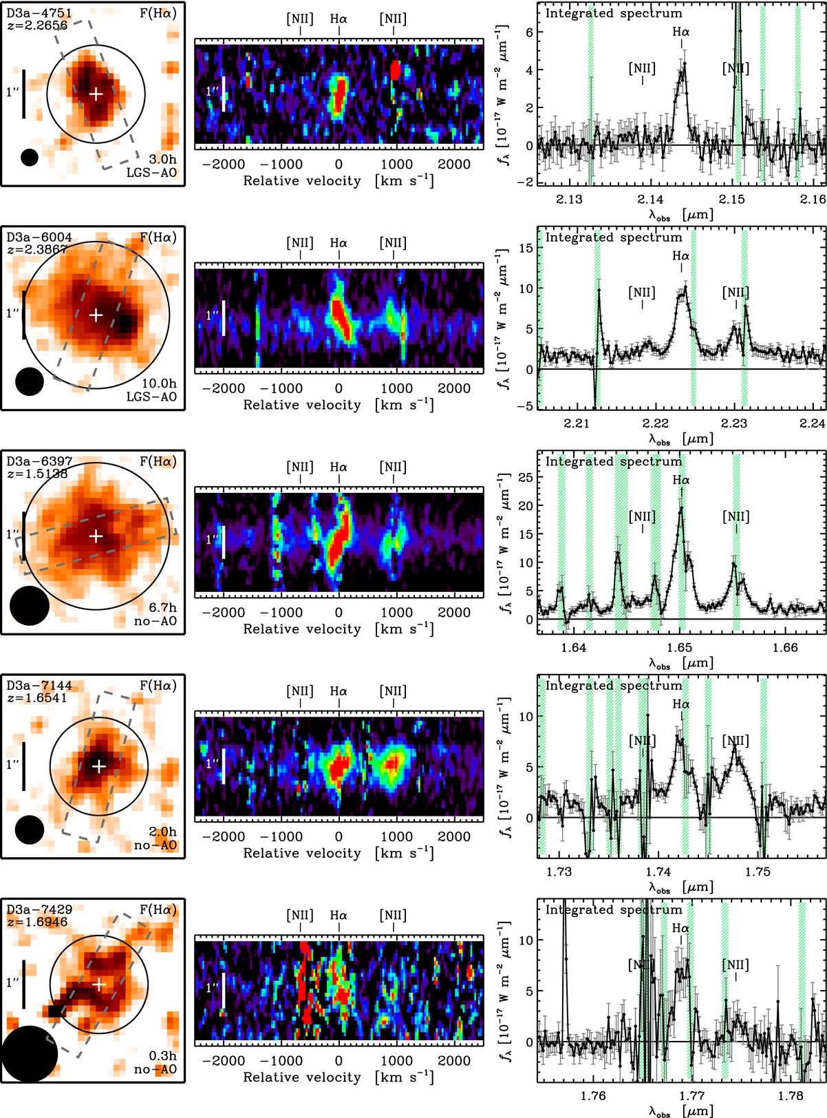
Figure 34. Same as Figure 22 for K-selected galaxies of the SINS Hα sample drawn from the GDDS survey.
Download figure:
Standard image High-resolution image
Footnotes
- *
Based on observations obtained at the Very Large Telescope (VLT) of the European Southern Observatory, Paranal, Chile (ESO Programme IDs 070.A-0229, 070.B-0545, 073.B-9018, 074.A-9011, 075.A-0466, 076.A-0527, 077.A-0576, 078.A-0055, 078.A-0600, 079.A-0341, 080.A-0330, 080.A-0635, and 080.A-0339).
- 20
Thus excluding, e.g., Spitzer/MIPS 24 μm flux-limited samples; although MIPS observations were carried out for many of the survey fields from which we drew our SINS targets, none of them were MIPS-selected.
- 21
The undetected GMASS sources include four of the irregular and multi-component systems and the two unresolved sources; the observations were taken under poorer than average seeing conditions, reducing the sensitivity for compact sources and/or subcomponents.
- 22
These and additional imaging data to help prepare the SINFONI observations were kindly provided by I. Smail, S. Chapman, and R. Ivison.
- 23
The G bandpass has an effective wavelength ≈4800 Å close to that of the various B bands at ≈4400 Å, and the color term is expected to be small compared to the measured colors of the galaxies.
- 24
For the different model assumptions considered in Appendix A, the changes in ensemble properties for the SINS Hα and CDFS samples are comparable, so that the relative differences and ranges between the two samples remain approximately the same. The median values for the SINS Hα sample using the Maraston (2005) models vary as follows: the stellar mass decreases by ≈25% to M⋆ = 2.0 × 10¹⁰ M☉, the stellar age becomes roughly twice younger or 130 Myr, the AV is higher by 0.2 mag, and the median absolute and specific SFRs increase by factors of 1.8 and 2.7, respectively, to SFR = 127 M☉ yr−1 and sSFR = 7.8 Gyr−1.
- 25
This is unchanged when using the SED modeling results for the other assumptions considered in Appendix A, and is verified with the Mann–Whitney U-test.
- 26
We note that the diffraction-limited scale of SINFONI, with pixel size of 12.5 mas and FOV of 0
8 × 08, is not suitable for our faint high-redshift targets with spatially extended emission because the smaller pixel scale results in too large read-noise penalty and the FOV is generally insufficient to cover the entire source. - 27
More generally, for other lines that are also detected in our data, we fixed the wavelength and width to those implied by the redshift and width of Hα. Fixing these parameters helped in extracting fluxes for lines in spectral regions affected by higher noise levels and/or that are intrinsically weaker but still detected. In most cases, we found that these assumptions were generally appropriate.
- 28
This holds also when using the stellar masses derived with the different SED modeling assumptions considered in Appendix A.
- 29
Other SED modeling assumptions (see Appendix A) lead to similar slopes within 5% of unity, and similar standard deviations of residuals of 0.13–0.19 dex.
- 30
The resonantly scattered Lyα line is very sensitive to radiative transfer effects, which complicates its use to constrain the dust obscuration.
- 31
Differences are small compared to the scatter of our data and qualitatively of no consequence for the discussion presented here.
- 32
Ranges in median values are, for other SED modeling assumptions, 0.3–0.9 and 0.9–1.3 for the cases without and with extra attenuation.
- 33
The median and ranges vary for the other SED modeling assumptions by up to factors of ≈3 for SFR(SED) as well as SFR0(Hα) and SFR00(Hα) (because the extinction correction is based on the best-fit AV from the SED modeling) but in all cases, the SFR0(Hα)'s are overall significantly lower than the SFR(SED)'s (by ≈30% to a factor of ∼4) while applying the extra attenuation leads to SFR00(Hα)'s in better agreement with SFR(SED)'s (to ⩽30%) with 1.3–1.5 times lower scatter in the relationship.
- 34
Changes in our SED modeling assumptions affect the zero point and scatter of the M⋆–SFR relationship by factors of ∼2–3; the resulting best-fit slopes have a power-law index consistent with unity to ±0.25 dex.
- 35
These are D3a-7429, GMASS-2454, GMASS-2550, ZC-772759, and SA12-8768NW.
- 36
This compares reasonably well with Épinat et al. (2009), who determined the vrot/σ0 in a similar way for their SINFONI sample at 1.2 ≲ z ≲ 1.6, and for which two of their nine sources have a ratio <1.
- 37
- 38
The WIRCAM Ks photometry was kindly made available to us in advance of publication.
- 39