


ABSTRACT
The Voyager 2 plasma observations of the proton distribution function downstream of the quasi-perpendicular heliospheric termination shock (TS) showed that upstream thermal solar wind ions played little role in the shock dissipation mechanism, being essentially transmitted directly through the shock. Instead, the hot supra-thermal pickup ion (PUI) component is most likely responsible for the dissipation at the TS. Consequently, the downstream proton distribution function will be a complicated superposition of relatively cool thermal solar wind protons and hot PUIs that have experienced either direct transmission or reflection at the TS cross-shock potential. We develop a simple model for the TS microstructure that allows us to construct approximate proton distribution functions for the inner heliosheath. The distribution function models are compared to κ-distributions, showing the correspondence between the two. Since the interpretation of energetic neutral atom (ENA) fluxes measured at 1 AU by IBEX will depend sensitively on the form of the underlying proton distribution function, we use a three-dimensional MHD-kinetic global model to model ENA spectra at 1 AU and ENA skymaps across the IBEX energy range. We consider both solar minimum and solar maximum-like global models, showing how ENA skymap structure can be related to global heliospheric structure. We suggest that the ENA spectra may allow us to probe the directly the microphysics of the TS, while the ENA skymaps reveal heliospheric structure and, at certain energies, are distinctly different during solar minimum and maximum.
Export citation and abstract BibTeX RIS
1. INTRODUCTION
IBEX (McComas et al. 2004, 2006, 2009a), launched on 2008 October 19, is measuring the energetic neutral atom (ENA) flux from the boundary regions of our heliosphere. Contemporaneously, Voyager 1 and 2 (V1, V2) are making in situ measurements of plasma, energetic particles, and magnetic fields along two trajectories in the heliosheath (Stone et al. 2008; Richardson et al. 2008; Decker et al. 2008; Burlaga et al. 2008; Gurnett & Kurth 2008). The interpretation of the IBEX observations will depend critically on global simulations of the solar wind–local interstellar medium (LISM) interaction (Heerikhuisen et al. 2008), informed by in situ data returned by the Voyager spacecraft. Underlying the determination of the ENA flux observed at 1 AU is the form of the proton distribution function in the inner heliosheath. ENAs are created by charge exchange of interstellar neutral H and heliosheath (inner and outer) protons or ions. Because the inner heliosheath is hot, a population of ENAs is created. The flux of ENAs will therefore depend quite sensitively on the number of particles in the wings of the hot proton population downstream of the heliospheric termination shock (TS), something recognized by both Prested et al. (2008) and Heerikhuisen et al. (2008) in their introduction of a κ-distribution to model the inner heliosheath proton distribution. In particular, in an important extension of their earlier work, Heerikhuisen et al. (Heerikhuisen et al. 2008) developed a fully self-consistent three-dimensional MHD-kinetic neutral hydrogen (H) model describing the solar wind-LISM interaction (Pogorelov et al. 2006, 2007, 2008a) using a κ-distribution to describe the underlying proton distribution in the heliosheath. Previous models assumed a Maxwellian description for the protons with self-consistent coupling to interstellar neutral H—the self-consistent coupling being crucial in determining the global heliospheric structure (Baranov & Malama 1993; Pauls et al. 1995; Zank et al. 1996b; Pogorelov et al. 2006—see, Zank 1999; Zank et al. 2009; Pogorelov et al. 2009c for extensive reviews). Prested et al. (2008) by contrast used a test particle approach to model the neutral H production based on an ideal MHD model.
The treatment of the heliospheric proton distribution function as a κ-distribution yields important differences in both the global structure of the heliosphere (decreasing the overall extent of the inner heliosheath between the TS and the heliopause) and the predicted ENA flux at 1 AU (Heerikhuisen et al. 2008). By assuming a κ-distribution with index κ = 1.63 (this motivated by the observed spectral index associated with energetic particles downstream of the heliospheric TS; Decker et al. 2005), Heerikhuisen et al. (2008) find that the ENA flux at 1 AU is substantially higher than for a corresponding Maxwellian proton distribution with the same temperature. This is not especially surprising of course because the κ-distribution contains many more particles in the wings of the distribution than the corresponding Maxwellian, thereby giving higher fluxes of ENAs at higher energies. Why the heliosheath proton distribution function should be like a κ-distribution with a spectral index close to 1.63 is however quite unclear. The answer may well reside in the processing of the upstream pickup ion (PUI) distribution by the TS and the subsequent statistical relaxation of the processed distribution in the heliosheath (Livadiotis & McComas 2009). IBEX will soon provide definitive observations of the ENA flux at 1 AU that will allow us to estimate the proton distribution in the inner heliosheath.
Related to the question of the heliosheath proton distribution are the plasma and magnetic field observations made by Voyager 2 on the second crossing of the TS. V2 has a working plasma instrument and the coverage was sufficient to identify three distinct crossings of the TS and make in situ measurements of the microstructure. The identified TS-3 crossing revealed an almost classical perpendicular shock structure (Burlaga et al. 2008; Richardson et al. 2008). However, plasma measurements revealed that the solar wind proton temperature changed from ∼20,000 K upstream to ∼180,000 K downstream (Richardson et al. 2008; Richardson 2009). Although hot solar wind plasma is sometimes observed, the average downstream proton plasma temperature is an order of magnitude smaller than predicted by the MHD Rankine-Hugoniot conditions, and the global self-consistent models all yield downstream proton temperatures of ∼2 × 10⁶ K (Zank et al. 2009). The downstream shock heated solar wind ion temperature observed by V2 is in fact so low that the downstream flow appears to remain supersonic (Richardson et al. 2008). Furthermore, the transmitted solar wind proton distribution appears to be essentially a broadened/heated Maxwellian (with a somewhat flattened peak), and there is no evidence of reflected solar wind ions being transmitted downstream (Richardson 2009). Richardson et al. (2008) and Richardson (2009) concluded that PUIs experienced preferential heating at the TS and thus provided both the primary shock dissipation mechanism and the bulk of the hot plasma downstream of the TS. Unfortunately, the Voyager spacecraft were not instrumented to measure PUIs directly. That PUIs provide the TS dissipation and heated downstream plasma had in fact been predicted by Zank et al. 1996b in their investigation of the interaction of PUIs and solar wind ions with the TS. They concluded that "P[U]Is may therefore provide the primary dissipation mechanism for a perpendicular TS with solar wind ions playing very much a secondary role." Thus the basic model of Zank et al. (1996b) for the microstructure of the TS appears to be supported by the V2 observations. However, both the observed solar wind proton distribution and a shock dissipation mechanism based on PUIs means that the downstream proton distribution function is a (possibly complicated) function of the physics of the TS. The purpose of this work is to present a basic model of the quasi-perpendicular TS, mediated by PUIs, that allows us to derive the complete downstream proton distribution function in these regions, the partitioning of energy between solar wind protons and PUIs, and infer potential implications of these results for the ENA flux observed at 1 AU in terms of spectra and skymaps. We do not attempt to synthesize a complete description of the heliosheath proton distribution at this point, preferring instead to elucidate the physics of the quasi-perpendicular TS, and relate that physics to the production of ENAs. Other regions of the TS, notably the high polar regime and possibly the heliotail region of the TS, may require the introduction of distinctly different physical processes for shock dissipation, and a complete model of the heliosheath proton distribution will therefore need to account for multiple shock regimes. In some respects, the recent IBEX observations are a little different in detail from those modeled here. In part, this stems from our using somewhat generic models for the large-scale heliosphere, both during solar maximum and solar minimum-like conditions (McComas et al. 2009b; Schwadron et al. 2009; Funsten et al. 2009). Nonetheless, the focus here is not to try and reproduce the IBEX observations but rather to develop a model or paradigm within which to incorporate the Voyager 2 TS observations and address the potential implications for the IBEX observations. As we show, these implications are that inner heliosheath proton spectra may be more complex than simple power laws and that consequently the ENA spectra may possess some structure (which appears to be the case but much more analysis of the data is needed). This work provides a framework within which to explore ENA spectra, and we will incorporate these results in a detailed comparison of IBEX data in the future. In this paper, we also consider the differences in the ENA fluxes expected of solar minimum and solar maximum-like conditions for two orientations and strengths of the interstellar magnetic field.
2. TS MODEL
In the supersonic solar wind, interstellar neutral H (and other species) is ionized by charge exchange, creating a beam of hot (∼1 keV) ions. The beam is unstable to the generation of Alfvén waves, on which the PUIs subsequently scatter. In this way, a bispherical distribution (well approximated by a shell distribution) for PUIs results (Williams & Zank 1994). The PUI shell convects at the background solar wind speed, experiencing adiabatic cooling with increasing heliocentric distance. Since shell distributions are created at all radial distances beyond the ionization cavity, the complete PUI distribution in the supersonic solar wind is a filled shell, expressed in the solar wind flow frame as (Vasyliunas & Siscoe 1976)
where c is the particle speed in the solar wind frame, c = |c|, np the PUI number density, and u = |u| is the solar wind bulk speed. The pressure contributed by PUIs is therefore
where mi is the proton mass. Because the energy gained in the pick-up process is proportional to u2, the PUI pressure dominates in the outer heliosphere, and this is reflected in the pressure/temperature distributions in the global heliospheric models (Pogorelov et al. 2008a; Heerikhuisen et al. 2008; Zank et al. 2009). From the plasma observations made by V2 upstream of the TS, we can estimate the PUI temperature in the supersonic solar wind just ahead of the shock. Using the observed plasma and magnetic field data just ahead of the shock (nSW = 0.001 cm−3, uSW = 300 km s−1, TSW = 20, 000 K, and B = 0.05 nT), and assuming conservatively that PUIs are 20% of the total ion population, i.e., np = αni, α = 0.2 and ni denotes the total number density, we estimate the upstream PUI temperature Tp to be
and the subscript 1 (2) denotes the value upstream (downstream) of the TS. Since the upstream total temperature T1 is

we find T1 ≃ 3.4 × 10⁵ K, assuming that the electron temperature and solar wind proton temperature are equal (∼20,000 K). Here TSW is the solar wind temperature. This estimate is consistent with the self-consistent MHD simulations of Pogorelov et al. (2008a) and Heerikhuisen et al. (2008). The inclusion of PUIs implies that the solar wind plasma beta is large, βSW = 4.3.
The primary dissipation mechanism at quasi-perpendicular shocks is the reflection of some incident ions by the electrostatic cross-shock potential. The cross-shock potential, formed as a result of the overshoot of protons as protons and electrons are decelerated abruptly at the shock, is associated with the steepest section of a quasi-perpendicular shock, viz., the ramp. The reflected protons are trapped ahead of the quasi-perpendicular shock, gaining energy from the upstream motional electric field, until the particle Lorentz force is large enough to overcome the electrostatic cross-shock potential barrier. The region ahead of the shock ramp, where the reflected ions are trapped, forms the shock foot—the pressure induced by the reflected protons causes a weak deceleration of the flow ahead of the ramp. Voyager 2 observed a textbook example of perpendicular shock structure on the third crossing of the TS, identified as TS-3, and the characteristic foot, ramp, and post-shock overshoot/undershoot were clearly identifiable.
Although exceedingly difficult to determine accurately using a set of single spacecraft measurements, especially in the absence of PUI data and the difficulty in establishing the shock speed (and disentangling that from the intrinsic shock motion), a Rankine—Hugoniot analysis indicates that the TS observed by V2 was quasi-perpendicular (Li et al. 2008; Burlaga et al. 2008) and moving inward at about 65 km s−1. Burlaga et al. (2008) estimate a shock ramp thickness of about 5500 km and a foot thickness of about 63,500 km. The ramp itself exhibited fine-scale structure on the order of 1000 km. For a PUI upstream of the TS, the PUI gyroradius is ∼60,000 km, which is consistent with the inferred foot thickness, and much greater than the inferred ramp and ramp fine-scale structure. The ion inertial length is c/ωpi ∼ 7100 km.
As discussed by Zank et al. (1996b) and Lee et al. (1996), protons with velocity vx in the shock frame such that
are reflected by the cross-shock potential ϕ (where E = −∇ϕ,  is the direction normal to the perpendicular shock front and
  is in the plane of the shock front). From Equation (4), we can define a threshold velocity
  such that protons with vx < Vspec in the shock frame will experience specular reflection at the cross-shock potential. PUIs, by virtue of their filled-shell distribution with radius in phase space of u (the solar wind speed), occupy a large part of phase space that satisfies this condition compared to the cold solar wind proton Maxwellian distribution—this is illustrated in Figure 1, where a projection of the phase space distribution is plotted in the two-dimensional (vx, vz)-plane, normalized to the upstream flow speed u1. Here, vx and vz are particle velocities perpendicular and parallel to the upstream mean magnetic field in the shock frame. The vertical line identifies a reasonable value of
  , showing that, unlike the PUI distribution, virtually no solar wind protons can be reflected.

Figure 1. Phase space plots of the filled-shell PUI distribution (left panel) and solar wind proton Maxwellian distribution (right) in the solar wind just ahead of the heliospheric TS, projected onto the velocity space coordinates (vx, vz) (perpendicular and parallel to the mean magnetic field) and normalized to the upstream bulk solar wind speed u1. The color coding refers to the number density. The distributions are plotted in the TS frame and the vertical line corresponds to a reasonable value of Vspec.
Download figure:
Standard image High-resolution imageTo determine the heliosheath proton distribution function, we consider separately the solar wind protons and the transmitted and reflected PUI distribution. For the solar wind protons, in view of Figure 1, we shall assume that all are transmitted downstream and that they do not contribute to the reflected proton distribution. We further assume that the solar wind proton distribution is a Maxwellian. Since the number of PUIs reflected is comparatively small (shown below specifically), we shall make the simplifying assumption that the non-reflected PUI distribution can be approximated by the filled-shell distribution (1) with number density ntp,1 (this is probably quite reasonable in view of phase mixing). On integrating the stationary transport equation for PUIs in the flow frame

across the shock, we have u1f1(c) = u2f2(c), or equivalently that the downstream distribution is simply
where r = u1/u2 is the shock compression ratio. Expression (5), with the appropriate ntp,1, yields part of the downstream proton distribution, which will be a superposition of the transmitted solar wind, the transmitted PUI, and the downstream reflected PUI distributions.
To estimate the energy gained by a particle transmitted across the TS, we must account for the proton deceleration by the cross-shock potential, thus
We Taylor expand this expression about the upstream flow speed u1 and use  to find

By taking the scalar pressure moment of the transmitted PUIs and using Equation (7) yields Ptp,2 = r3Ptp,1, or
This result holds for arbitrary isotropic distributions at an idealized shock discontinuity. For r = 2.5, as observed at TS-3, and Tp,1 = 1.56 × 10⁶ K, we have Ttp,2 = 9.75 × 10⁶ K for the transmitted PUIs. Expression (8) also yields a downstream solar wind proton temperature TSW,2= 125,000 K, which is quite close to the observed downstream solar wind temperature (see Figure 3 of Richardson 2009 which shows a temperature plateau from ∼40, 000–180, 000 K).
To estimate the temperature of the downstream reflected PUIs, we note (Zank et al. 1996a) that reflected PUIs are trapped at the perpendicular shock front by a balance of the Lorentz force evyBz and the cross-shock potential gradient −eEx. Then, approximating eϕ ∼ 1/2miu21 (Zank et al. 1996a) (see above), we estimate the velocity vy gained by a PUI in the upstream motional electric field as
where rg1 is the gyroradius of an upstream PUI. Evidently, the energy gain is large provided Lramp ≪ rg1. On using values observed by Voyager 2, rg1 ∼ 63, 000 km, which is much greater than the observed ramp thickness of ∼5, 500 km (Burlaga et al. 2008). Thus, we find that
which yields an estimate for the downstream temperature of reflected PUIs as
Thus, Voyager 2 observations and the estimates above yield Trefp,2 ∼ 7.7 × 10⁷ K for the reflected PUI temperature transmitted downstream.
Finally, to estimate the number densities of the transmitted and reflected PUIs, we assume a filled-shell distribution and slice off that section corresponding to particles with vx ⩽ Vspec. This procedure yields
We may therefore estimate the total temperature downstream of the quasi-perpendicular TS using Equations (8), (10), (11a), and (11b) on the assumption that np1 = 0.2ni1, finding that
Such a total temperature is consistent with the post-shock temperatures obtained from self-consistent global MHD-kinetic simulations of heliospheric structure (i.e., models that incorporate charge exchange source terms in the conservation equations; Pogorelov et al. 2008a; Heerikhuisen et al. 2008; Zank et al. 2009), giving us confidence that the detailed shock microphysics is translating accurately into the MHD conservation laws.
3. APPLICATION TO GLOBAL MHD-KINETIC MODELS AND INFERRED ENA FLUXES: RESULTS AND DISCUSSION
The partitioning of downstream thermal energy into transmitted solar wind protons, transmitted PUIs, and reflected PUIs can be estimated from the foregoing section. Let T2 be given by simulations and express the temperature partitioning according to
and ΓSW = TSW/T2, etc. By way of illustration, on using the estimated value T2 = 3.4 × 10⁶ and the results of Section 2, we find ΓSW ∼ 6 × 10⁻², Γtp ∼ 2.9, and Γrefp ∼ 22.6, giving a downstream temperature/energy partition of ∼4.8% in solar wind protons, 52% in transmitted PUIs, and 45% in reflected PUIs. Clearly, PUIs, both transmitted and reflected, dominate the thermal energy content in the heliosheath, just as PUIs do upstream of the TS.
It is important to emphasize again that the one-fluid plasma description used in both our self-consistent MHD models (see, Zank et al. 2009 for a review) and others (e.g., Izmodenov et al. 2005) contains both solar wind ions and PUIs, even though a separate equation for PUIs is not included. Charge exchange between solar wind ions, PUIs, and interstellar H is included in the models, through both the conservation of momentum and total energy equations with appropriate source terms. The temperature/pressure in the self-consistent models contains the contribution of both the core solar wind ions and the PUIs, and correctly computes the total temperature/pressure. However, the total temperature/pressure cannot be separated within the context of a single fluid plasma description. To estimate the relative contribution of solar wind protons and PUIs to the total pressure requires additional assumptions about the physics of the problem, but the sum of the individual pressure is constrained to satisfy the total computed pressure obtained from simulations that are based on conservation laws.
We can use our suite of self-consistent global MHD-kinetic simulations of heliospheric structure to approximate the total proton distribution function at any location and time in the heliosheath. By partitioning the thermal energy content of the plasma in each computational cell according to the algorithm above, we can construct a local proton distribution by superimposing the appropriate transmitted solar wind, transmitted PUI, and downstream reflected PUI distributions. We consider two limiting possibilities. In the first, we suppose that the transmitted solar wind, transmitted PUI, and downstream reflected PUI distributions can all be regarded as Maxwellian distributions with the appropriate number densities and temperatures, and of course that they all continue to co-move with the background flow. For the second limiting case, we suppose that the transmitted PUI distribution preserves its filled-shell character, i.e., we use expression (5). This is supported by the simulations of Burrows 2008, and Burrows et al. 2009, who calculated the transmission of an upstream filled-shell PUI distribution across the TS. They found that the transmitted PUIs tend to preserve their approximately filled-shell distribution downstream of the shock. Like Heerikhuisen et al. (2008), we use a three-dimensional MHD-kinetic simulation based on a κ-distribution for the heliosheath plasma, but we consider both solar minimum and solar maximum-like (i.e., a more-or-less isotropic solar wind but without the highly disturbed character of the wind) conditions. A detailed discussion of the former model has been given by Heerikhuisen et al. (2008), and the latter is discussed by Pogorelov et al. (2008a). Our models are based on the Multi-Scale Fluid-Kinetic Simulation Suite (MS-FLUKSS) described in Pogorelov et al. (2008b), and uses the kinetic neutral hydrogen code developed by Heerikhuisen et al. (2006). The model treats the proton population as a single fluid whose total pressure is given by the sum of the thermal solar wind protons and electrons and the PUIs. Because the pickup of interstellar neutral H yields a PUI population that co-moves with the bulk solar wind flow, a single fluid plasma model captures exactly the energetics and dynamics of the combined solar wind/PUI plasma. The pickup of protons and creation of neutral H atoms is included self-consistently through source integrals in the plasma momentum and energy equations (Pauls et al. 1995) and neutral H Boltzmann equation (Heerikhuisen et al. 2006). In a simplified approach devised to add a power-law tail to the proton population, Heerikhuisen et al. (2008) introduced a κ-distribution to describe the heliosheath plasma with an index κ = 1.63, the choice being motivated by V1 Low Energy Charged Particle data reported by Decker et al. (2005). We use two possible models of the heliosphere. In the first, we assume solar minimum-like conditions with high speed, low density, relatively hot wind over the poles and low speed, higher density, lower temperature wind in the ecliptic. For the supersonic solar wind boundary conditions at 1 AU, we assume for the slow wind in the ecliptic: uSW = 400 km s−1, TSW = 105 K, np,SW = 7 cm−3 (proton density); and for the fast polar wind: uSW = 800 km s−1, TSW = 2.6 × 10⁵ K, np,SW = 2.6 cm−3, and finally the radial component of the IMF at 1 AU is 37.5 μG. The LISM boundary conditions are taken as VLISM = 26.4 km s−1, TLISM = 6527 K, np,LISM = 0.05 cm−3, LISM neutral H number density nH = 0.15 cm−3, magnetic field magnitude |B| = 1.5 μG, and B belongs to the meridional plane and is at 30° to the LISM velocity vector, being directed into the southern hemisphere. For the second case, we consider solar maximium-like conditions in that we assume a constant solar wind speed, density, and temperature at the 1 AU base for all heliospheric latitudes and longitudes. This of course neglects the highly dynamical state of the solar wind during solar maximum. The dynamical solar wind strongly affects the location of the TS and state of the inner heliosheath (Zank & Müller 2003; Washimi et al. 2007; Pogorelov et al. 2009a). At 1 AU, we use the following parameters for the supersonic solar wind (Pogorelov et al. 2009b, 2008a): uSW = 450 km s−1, TSW= 51,100 K, np,SW = 7.4 cm−3 (proton density). For the LISM conditions, we use the same as above except that np,LISM = 0.06 and the interstellar magnetic field is stronger |B| = 3 μG and lying in the hydrogen deflection plane (Lallement et al. 2005). We note that the change from solar minimum to maximum and back again will lead to mix of timescales—the plasma timescale for restructuring of the heliosphere must incorporate the response of the global structure to the varying solar wind ram pressure, magnetic field, temperature, and density, and of course the propagation of low energy and high energy neutral H through the heliosphere introduces new (long and short) timescales that modify the gross heliospheric characteristics. Ideally, we should run a fully time-dependent simulation that allows us to follow the full evolution of the heliosphere, including neutral H self-consistently, and this would then allow us to apply the more complicated inner heliosheath proton distribution model to the problem. Unfortunately, this is currently impractical and so we have compromised by using a somewhat generic snapshot of a three-dimensional model that reflects crudely solar minimum-like or solar maximum-like conditions.
Figure 2 shows the global structure of the heliosphere during solar maximum (top) and minimum (bottom), where the plasma temperature is plotted in the ecliptic and meridional planes. The top two panels of Figure 2 show that the structure during solar maximum is relatively featureless, at least on sufficiently large global scales. An obvious asymmetry from nose to tail is evident. However, as illustrated in the meridional cut, Figure 2(a), a substantial northward asymmetry exists in the thickness of the heliosheath. This is due to the northward bending of the current sheet—the supersonic flow above the current sheet is bent sharply northward at the TS to stay above (now inside) the current sheet. Part of the supersonic solar wind that was south of the current sheet also flows northward, but behind the current sheet in the inner heliosheath. Thus, transverse flows in the north and south regions of the inner heliosheath are substantially different, and because part of the southern latitude plasma is convected northward, the northern inner heliosheath is broader than the southern region. This yields a longer line of sight for the creation of ENAs. Figure 2 illustrates the complex meridional structure of the heliosphere during solar minimum. The fast, hot polar solar wind dominates the global structure of the heliosphere, although partially offset by the slightly higher neutral H flux at high latitudes (Pauls & Zank 1997, Zank 1999, and Pogorelov et al. 2008a). The structure exhibited in the supersonic solar wind persists into the inner heliosheath, with the plasma remaining divided into essentially two thermodynamically distinct regions, this due to the distinct character of the supersonic solar wind in the polar and ecliptic regions inducing differences in the TS strength. A further asymmetry in the north–south is present due to the current sheet bending northward and creating a slightly thicker heliosheath in the north, while LISM magnetic pressure tends to squeeze and narrow the southern heliosheath. The presence of a rather pronounced heliosheath asymmetry and corresponding structure should manifest itself in ENA skymaps since hotter regions will produce an excess of ENAs. By contrast, the ecliptic regions during both solar minimum and maximum (right panes of Figure 2) are more symmetric. Finally, we note the significant differences in heliotail structure, both in the meridional and ecliptic planes, for solar minimum and maximum conditions. These differences may manifest themselves in a solar cycle dependence in the ENA skymaps.
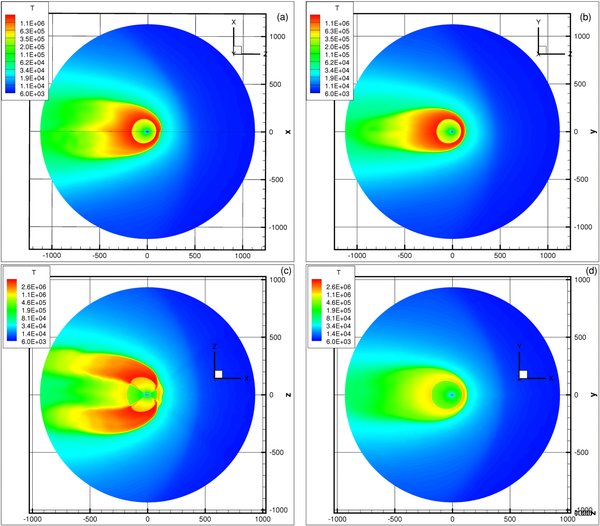
Figure 2. Three-dimensional structure of the global heliosphere used to determine the heliosheath plasma distributions. The plots show the logarithmic plasma temperature in the meridional (left) and ecliptic (right) planes for solar minimum conditions.
Download figure:
Standard image High-resolution imageWe introduce the energy partition derived above to determine the relative contribution to the total plasma energy from transmitted solar wind protons, transmitted PUIs, and downstream reflected PUIs for both cases. Because of the differing TS and consequently inner heliosheath plasma properties with latitude, the energy partitioning will be a function of latitude.
Shown in Figure 3 are examples of the heliosheath proton distribution, using on the left, the assumption that the transmitted PUIs relax to a Maxwellian distribution, and, on the right, that the transmitted PUIs remain a filled-shell distribution. A corresponding κ-distribution is plotted with index 1.63, together with a downstream total Maxwellian. Evidently, the κ-distribution resembles a smoothed form of both constructed heliosheath proton distributions. Moreover, both forms of the constructed distributions exhibit the important property that a significant number of protons reside in the wings of the distribution function, quite unlike the Maxwellian distribution. There are several noteworthy points about the distribution functions plotted in Figure 3. The first is the narrowness of the transmitted solar wind proton distribution, the second is the broadening of the distribution function by the transmitted PUIs out to about 5vth (where vth is the thermal velocity corresponding to a Maxwellian distribution with temperature T, in this case the total downstream plasma temperature), and finally the downstream reflected PUIs considerably extend the outermost wings of the total proton distribution function. The filled shell assumption for the transmitted PUIs probably overestimates the hardness of the spectrum, and we would expect the spectrum to be intermediate to the two cases illustrated in Figure 3. Nonetheless, the close correspondence between the constructed distributions and the κ-distribution with index 1.63 is quite remarkable. However, it is important to recognize that the constructed heliosheath proton distribution, under both assumptions for the transmitted PUIs, possesses some structure that may manifest itself in ENA spectra observed at 1 AU by IBEX. We therefore suggest that the microphysics of the TS may play a key role in determining the form of the total downstream or heliosheath proton distribution.

Figure 3. Plots of the local proton distribution function in the heliosheath. The blue curve shows the κ-distribution used by Heerikhuisen et al. (2008) with a value of −1.63. The black curves depict the distribution constructed from a superposition of the transmitted solar wind protons, the transmitted PUIs, and the downstream reflected PUIs. The red curve illustrates a Maxwellian distribution with the downstream density and temperature. (Left) The heliosheath constructed proton distribution (black curve) assuming that the transmitted PUIs evolve into a Maxwellian distribution. (Right) The heliosheath constructed proton distribution (black curve) assuming that the transmitted PUIs possess a filled-shell distribution. The particle velocity vx is normalized to the Maxwellian thermal speed vth = 2kT/mi where k is Boltzmann's constant and T is the total downstream temperature.
Download figure:
Standard image High-resolution imageWe can use the constructed distribution functions, illustrated in Figure 3, directly in our various global MHD-kinetic simulations (Pogorelov et al. 2008a) to evaluate the ENA flux at 1 AU and determine the skymaps at different energies. The differential intensity at 1 AU emanating from the nose (top), flank (middle), and tail (bottom) directions assuming (left column) that the transmitted PUIs form a Maxwellian distribution downstream or (right column) a filled-shell distribution is shown in Figure 4. The contribution from the individual components that make up the heliosheath proton distribution are plotted separately; blue shows ENAs created by charge exchange with transmitted solar wind protons, green with transmitted PUIs, and red with downstream reflected PUIs. The total composite flux is identified by the black line. For the purposes of comparison, the purple line corresponds to the ENA flux generated by a proton κ-distribution with κ = 1.63. Evidently, the overall intensity in ENA flux from the κ- and constructed proton distributions agrees very well over the entire energy range up to about 10 keV. Up to about 2 keV, the overall ENA spectrum is clearly dominated by H atoms created from transmitted PUIs, and above 2 keV by ENAs created from downstream reflected PUIs. As a result, the ENA spectrum from the TS microphysical model possesses some structure compared to the κ-generated ENA spectrum. If indeed spectral structure in the ENAs is measured by IBEX, one interpretation may well be that it reflects the microphysics of the TS. The results of Figure 4 suggest that the ENA flux at 1 AU in the nose direction will be dominated by transmitted PUIs in the 0.05–2 keV range and by heliosheath reflected PUIs in the 2–10 keV range. Thus, we may anticipate that the relative ENA intensity at 1 AU between these two ranges will provide time-averaged information about the detailed microphysical processes operating at the TS. Some structure in the ENA spectrum at 1 AU remains in the sidestream direction, although perhaps less pronounced than in the nose direction, but certainly more than exhibited in the heliotail direction. The heliotail ENA spectrum is considerably smoother with a double power-law-like structure with a break at ∼0.7 keV. The ENA spectrum generated by the heliotail proton distribution at lower energies is harder than the corresponding κ-distribution but is almost identical beyond the spectral break. This is an obvious consequence of the extent of the heliotail.
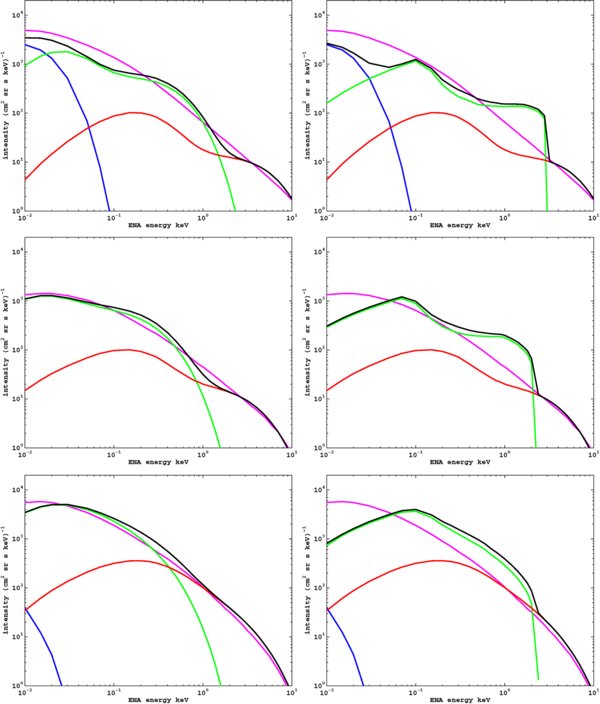
Figure 4. ENA energy spectra for solar minimum conditions at 1 AU along (a) the nose line of sight, (b) the ecliptic-sidestream, and (c) the heliotail direction. Each spectrum is a composite of contributions from the transmitted solar wind created ENAs (blue curve), the transmitted PUIs (green curve), and the heliosheath reflected PUIs (red curve). These spectra were derived assuming a Maxwellian distribution for the transmitted PUIs. The total or composite ENA spectrum is shown by the black curve, and the ENA spectrum generated by a κ-distribution with index 1.63 is identified by the purple curve. The left column assumes that the transmitted PUIs form a Maxwellian distribution downstream and the right column corresponds to the assumption of a filled-shell/power-law downstream distribution.
Download figure:
Standard image High-resolution imageThe right-hand column of Figure 4 illustrates ENA spectra at 1 AU in the same directions as those in the left column, but now under the contrasting assumption that the transmitted PUIs remain a filled-shell distribution. In view of the form of the constructed heliosheath proton distribution (hard spectrum, strong spectral break at ∼5 keV), the ENA features of the left column are now more exaggerated. All three directions exhibit clear spectral breaks that separate the transmitted PUI from the reflected PUI populations. In both cases, the transmitted thermal solar wind protons contribute very little to the ENA spectra at 1 AU.
The spectra shown in the two columns of Figure 4 illustrate a gradation in spectral features, from the featureless spectra generated by a proton κ-distribution, to the almost exaggerated features resulting from an assumed power-law spectrum for transmitted PUIs. If IBEX observes spectral features in the ENA distributions at 1 AU, we have illustrated how these can be interpreted in terms of the specific microphysics of the TS and the particular form of the heliosheath proton distribution. It is unlikely that IBEX will observe features quite as exaggerated as those in the right column of Figure 4 but they may well be intermediate to the two cases plotted here.
Illustrated in Figure 5 are plots corresponding to those of Figure 4 but now for solar maximum conditions. Small differences between solar minimum and maximum are discernable but the general conclusions above are unchanged.

Figure 5. Same as Figure 4 except that the ENA energy spectra were computed for solar maximum-like conditions at 1 AU. The left column assumes that the transmitted PUIs form a Maxwellian distribution downstream and the right column corresponds to the assumption of a filled-shell/power-law downstream distribution.
Download figure:
Standard image High-resolution imageFinally, we show in Figures 6–9 a series of skymap plots for four energies (50, 200, 2, and 5 keV), corresponding to solar minimum conditions. As above, we separate the contributions from the three proton components, and then create a composite plot that is compared to a skymap derived from the κ-distribution based plasma heliosheath model of Pogorelov et al. (2008a), following Heerikhuisen et al. (2008). We also employ the two approximations for the transmitted PUIs, viz., the Maxwellian and the filled-shell approximations. In each of the figures, the top panel of five figures (three figures in the left column, two in the right column) corresponds to the Maxwellian approximation for the transmitted PUIs, and the bottom panel of five figures to the filled-shell/power-law approximation.

Figure 6. All skymaps at 50 eV for solar minimum conditions. The top panel of five figures corresponds to an assumed Maxwellian downstream distribution for the transmitted PUIs, and the bottom panel of five figures to an assumed power-law distribution. Consider the top panel of five figures first. The ENA flux at 1 AU is measured in units of (cm−2 sr s keV)−1, and is generated by charge exchange in the inner heliosheath between interstellar neutral H and (left column, top) transmitted solar wind protons, (left column, middle) transmitted PUIs, or (left column, bottom) inner heliosheath reflected PUIs. (Right column, top) The total or composite ENA skymap, and (right column, bottom) the κ-distribution based skymap. The lower set of five panels corresponds to the top set of five except that the transmitted PUIs in this case are assumed to form a power-law distribution downstream. The direction of the LISM flow or nose direction is at the center of the plot, the poles are at the top and bottom, and the heliotail is at the far ends of the plot. Contour lines have been drawn at 15° intervals. Maps are generated by binning ENAs which intersect a sphere of radius 1 AU on radially inward trajectories.
Download figure:
Standard image High-resolution image
Figure 7. All skymaps of the 200 eV ENA flux at 1 AU in units of (cm−2 sr s keV)−1, using the Maxwellian (top five figures) and the power law (bottom set of five figures) approximation for the transmitted PUIs. Same format as Figure 6.
Download figure:
Standard image High-resolution image
Figure 8. All skymaps of the 2 keV ENA flux at 1 AU in units of (cm−2 sr s keV)−1, using the Maxwellian (top five figures) and the power-law (bottom set of five figures) approximation for the transmitted PUIs. Same format as Figure 6.
Download figure:
Standard image High-resolution image
Figure 9. All skymaps of the 5 keV ENA flux at 1 AU in units of (cm−2 sr s keV)−1, using the Maxwellian (top five figures) and the power-law (bottom set of five figures) approximation for the transmitted PUIs. Same format as Figure 6.
Download figure:
Standard image High-resolution imageAt 50 eV, Figure 6, the transmitted solar wind protons contribute in the nose direction, and the skymap exhibits a weak southward asymmetry and a split or bimodal structure. However, the ENA flux generated by transmitted solar wind protons at this energy is very low (less than ∼600 particles/(cm2 sr s keV)) because of the cold solar wind Maxwellian distribution. By contrast, transmitted PUIs produce the largest ENA flux at this energy, in excess of 2000 particles/(cm2 sr s keV) from the heliotail direction, and the skymap exhibits a bimodal and banded structure (a consequence of the separation of the solar wind into a high speed polar flow and a low speed ecliptic wind). Transmitted PUIs also create a northward feature in the nose direction of the skymap and two bands (north and south) in the ENA flux. The dominance of the northward feature in the skymap is due to the northward bending of the current sheet and the subsequent broadening of the heliosheath in the north. At the 50 keV energy, the contribution of heliosheath reflected PUIs to the ENA flux at 1 AU is about 1/2 that of the transmitted solar wind proton contribution and substantially less than that created by the transmitted PUI population. The skymaps corresponding to ENAs created by reflected PUIs exhibit heliotail and banded features. The composite skymap corresponds well with the κ-generated skymap, both in flux levels and structure. The κ-distribution based map exhibits a somewhat more uniformly distributed ENA flux than does the composite case, which has a slightly more dominating northward flux, but otherwise there are few major differences. The case with the power-law model is quite similar with respect to the heliotail regions but is noticeably different in the transmitted PUI generated ENA flux in the nose direction. In this case, the model predicts almost no ecliptic noseward flux and the skymap for the composite case is dominated by the heliotail contribution and the banding associated with the high speed solar wind. This is in marked contrast to the κ-distribution based model.
Consider first the top panel of figures in Figure 7. At 200 eV, transmitted solar wind protons create essentially no ENAs that reach 1 AU. The ENA flux at 200 eV is dominated by transmitted PUIs over heliosheath reflected PUIs by a factor of ∼2 to 1. Although the heliotail ENAs created by transmitted PUIs dominate, there is a quite strong, widely distributed ENA flux in the nose direction, with a northern asymmetry. The downstream reflected PUIs contribute to the skymap in the heliotail direction, and as a band across the sky, stronger in the north than the south, with the north band noticeably broadened. As before, the heliotail flux possesses a bimodal structure. At 200 eV, the composite skymap and the κ-distribution generated skymap are quite similar, both in flux levels and structure, with the κ-distribution map exhibiting a slightly stronger northern asymmetry. The complete skymap corresponding to the composite spectrum has a broad swathe with a weak north pole contribution.
By contrast, although dominated by the transmitted PUI created ENAs, the power-law assumption yields a skymap of distinct structure, Figure 7, bottom five panels. Contributions from the heliotail and north polar regions dominate so that the overall composite map possesses much more striking features than the more uniform κ-distribution generated map. The high fluxes associated with the features exhibited by the composite skymap result from assuming a hard power-law spectrum, which yields many more particles at these energies than even the κ-distribution.
As can be seen from the 2 keV maps, Figure 8, an interesting and important difference arises in the Maxwellian approximation (top panel) compared to the power-law approximation (bottom panel). The skymap for ENAs created from transmitted PUIs in the Maxwellian approximation possesses two broad bands at high latitudes, but with relatively low flux intensity compared to the reflected PUI created ENA contribution from the tail regions. The overall or combined skymap in the Maxwellian approximation is dominated by the tail contribution of ENAs from reflected PUIs and ENAs from the transmitted PUI population contribute rather weakly, forming a band at high latitudes. The composite Maxwellian and κ-distribution skymaps are quite similar in structure and flux. By contrast, the skymaps generated under the power-law or filled-shell approximation are dominated by the ENAs created from transmitted PUIs, both in the vicinity of the nose and in the tail. Two broad asymmetric bands are formed about the nose, and the downstream reflected PUI created ENAs are a factor of ∼2–3 smaller in flux than that of ENAs created from the transmitted PUI component. The total flux level of the ENAs in the composite skymap under the power-law approximation is significantly higher than either the composite Maxwellian case or the κ-distribution case, reflecting the very hard distribution of transmitted PUIs at the TS (Figures 3–5).
Like the 2 keV case, the 5 keV skymaps exhibit distinct differences between the Maxwellian and power-law approximations. In both cases, the flux and distribution of ENAs from reflected PUI created ENAs is the same, dominated by the heliotail contribution and a broad contribution from the nose region. However, the flux of the transmitted PUI created ENAs is ∼40 less in the case of the Maxwellian approximation but a factor of ∼2 greater in the power-law approximation. Thus the combined skymap in the Maxwellian approximation is dominated by reflected PUIs (and is very similar in both flux and structure to the κ-distribution based model) whereas the power-law approximation for transmitted PUIs yields a skymap dominated by transmitted PUIs instead (and ∼3 times greater flux levels overall for ENAs), originating from two bands at high north and south latitudes.
Finally, in Figure 10, we plot the composite skymaps for solar-maximum-like conditions. The left column corresponds to the Maxwellian approximation for the transmitted PUIs, and the right to the power-law or filled-shell approximation. Each row corresponds to a distinct energy for the ENAs (from top to bottom, 50, 200, 2, and 5 keV). As with the solar minimum cases, the overall ENA fluxes are significantly higher for the power-law approximation cases than the Maxwellian cases, at least below 5 keV. Structurally, the skymaps for solar minimum and maximum conditions in the Maxwellian approximation are different in that the solar minimum case, from 50 eV to 2 keV, exhibits pronounced banding, either at high latitudes or across the nose. The hot high-speed polar solar wind imposes itself clearly on the skymap fluxes. The flux at both solar maximum and minimum conditions with the Maxwellian approximation is very similar at 2 keV, but a factor of ∼2 less at 50 and 200 eV. The 5 keV "Maxwellian" skymap is somewhat similar for the two solar wind possibilities, except that the heliotail contribution to the ENA flux is more uniformly distributed than the bimodal structure exhibited during solar minimum and the nose contribution during solar maximum is smaller at the nose. The overall flux levels are almost identical. The power-law or filled-shell approximation yields skymaps that are structurally quite distinct between solar minimum and maximum conditions (no banded structure at 50 and 200 eV, a single strong northward band and broad heliotail contribution at 2 keV) and the fluxes are higher at 50 and 200 eV during solar maximum (by a factor ∼2.5) but similar at higher energies. However, unlike the solar minimum case, the skymaps at 5 keV in both the Maxwellian and power-law approximations are almost identical for solar maximum-like conditions. This is a result of the underlying proton spectrum about a 5 keV range being dominated by reflected PUIs during solar maximum and being approximated by a Maxwellian distribution. The hot higher speed polar solar wind during solar minimum ensures that some transmitted PUIs will contribute to the ENA flux near 5 keV energies. In summary, we may therefore anticipate that IBEX will observe structurally distinct skymaps during solar maximum-like conditions compared to the current solar cycle conditions.

Figure 10. All skymaps for the total or composite spectra models during solar maximum-like conditions. The left column corresponds to the total skymap derived from the Maxwellian approximation and the right column to the power-law approximation. In descending order, each row corresponds to the 50, 200, 2, and 5 keV ENA flux at 1 AU in units of (cm−2 sr s keV)−1.
Download figure:
Standard image High-resolution image
We may summarize our conclusions as follows.
- 1.We have developed a model describing the basic plasma kinetic processes and microphysics of the quasi-perpendicular TS in the presence of an energetic PUI population. We have shown that the solar wind protons do not experience reflection at the cross-shock potential of the TS, and are transmitted directly into the heliosheath. PUIs, by contrast, can be either transmitted or reflected at the TS, and provide the primary dissipation mechanism at the shock, and dominate the downstream temperature distribution. We have derived an inner heliosheath proton distribution function that is (1) consistent with V2 solar wind plasma observations, and (2) is similar to a κ-distribution with index 1.63. The latter result holds if we assume that the transmitted PUI distribution relaxes to either a Maxwellian or a filled-shell distribution.
- 2.The composite heliosheath proton distribution function is a superposition of cold transmitted solar wind protons, a hot transmitted PUI population, and a very hot PUI population that was reflected by the cross-shock electrostatic potential at least once before being transmitted downstream. The composite spectrum possesses more structure than the κ-distribution but both distributions have approximately the same number of protons in the wings of the distribution (and therefore many more than a corresponding Maxwellian distribution).
- 3.ENA spectra from various directions at 1 AU generated by either the composite (TS) heliosheath proton distribution or the κ-distribution are very similar in intensity, although some structure is present in the composite case. The spectral shape is a consequence of the contribution to the ENA flux by primarily heliosheath transmitted and reflected PUIs. The ENA spectrum is dominated by transmitted PUI created ENAs in the energy range below 2 keV and reflected PUI created ENAs in the range above 2 keV. This may give us an opportunity to use IBEX data to directly probe the microphysics of the TS.
- 4.Like the ENA spectra, the skymaps are dominated by ENAs created by either transmitted PUIs or reflected PUIs, depending on the energy range. The fluxes are determined by the relative contributions from the two PUI populations. The overall skymap structure at lower energies is quite similar for both the Maxwellian and power-law approximation cases, since the underlying proton distributions in both cases are very similar at this energy range. At higher energy ranges, where a noticeable difference between the two underlying proton distributions exists, the composite skymaps under the two approximations are noticeably different in fluxes and structure.
- 5.Finally, solar minimum should leave a distinctly different imprint on the skymaps than solar maximum, although the precise form will depend on whether the Maxwellian approximation or the filled-shell/power-law model is the better approximation.
We acknowledge the partial support of NASA grants NNX09AB40G, NNX07AH18G, NNG05EC85C, NNX09 - AG63G, NNX08AJ21G, NNX09AB24G, NNX09AG29G, and NNX09AG62G. Supercomputer time allocations were provided by NASA High-End Computing program award SMD-09-1148, Oak Ridge National Laboratory Director Discretion project PSS003, and NSF project MCA07S033 under the following NSF programs: Partnership for Advanced Computational Infrastructure, Distributed Terascale Facility (DTF), and Terascale Extensions: Enhancements to the Extendible Terascale Facility.