


ABSTRACT
The Michelson Doppler Imager on board the Solar and Heliospheric Observatory satellite has operated for over a sunspot cycle. This instrument is now relatively well understood and provides a nearly continuous record of the solar radius in combination with previously developed algorithms. Because these data are obtained from above Earth's atmosphere, they are uniquely sensitive to possible long-term changes of the Sun's size. We report here on the first homogeneous, highly precise, and complete solar-cycle measurement of the Sun's radius variability. Our results show that any intrinsic changes in the solar radius that are synchronous with the sunspot cycle must be smaller than 23 mas peak to peak. In addition, we find that the average solar radius must not be changing (on average) by more than 1.2 mas yr−1. If ground- and space-based measurements are both correct, the pervasive difference between the constancy of the solar radius seen from space and the apparent ground-based solar astrometric variability can only be accounted for by long-term changes in the terrestrial atmosphere.
Export citation and abstract BibTeX RIS
1. INTRODUCTION
The possibility that the Sun's radius varies is an important question, the answer to which has implications for our understanding of the static and dynamic structure of the solar interior. The first two papers in this series (Emilio et al. 2000, hereafter Paper I; Kuhn et al. 2004, hereafter Paper II) showed how the solar radius and its variation could be accurately inferred from the Michelson Doppler Imager (MDI) image time series. Our earlier analysis found no evidence of secular or cyclical radius changes at our detection level of about 9 mas yr−1 (Paper I) and 7 mas solar cycle−1 amplitude (Paper II).
The remarkable Solar and Heliospheric Observatory (SOHO)/MDI experiment has survived an entire solar cycle near the Earth–Sun Lagrange point. This allows the detection of solar-cycle radius changes with unprecedented accuracy. These data, combined with our good understanding of how small temperature changes in the MDI instrument affect the image scale, enable a refined understanding of possible solar radius variability. Now, with more than a solar cycle of accurate solar astrometry, we have strong limits on the possibility of solar-cycle radius changes.
We explored several algorithms, which are described in detail in Papers I and II, for obtaining the radius. In general, the solar radius is obtained from each image in several solar position angle sectors from the apparent solar limb darkening function (LDF) as seen through the MDI optics. Interpreting the absolute solar radius and reconciling measurements with models are difficult because the solar radius is not a well-defined observable, especially when interpreting kilometer and milliarcsecond model-observation differences. Haberreiter et al. (2007) have attempted to calibrate various empirical radius definitions against various models. We will avoid many of these problems by focusing on solar radius temporal variations, which we find to be largely independent of the details of the precise radius definition. In a future publication, we will discuss the difficult comparison of the static empirical and model solar radii. The empirical solar radius point is affected by the details of the algorithm and instrument changes that affect the apparent LDF. For example, as described in Paper II, we found that our limb definition showed significant spurious variability when the instrument was far from focus. Much of the first year MDI was operated far from best focus so that these early data will not be used in our analysis below.
Our tiny limits on radius variability described in Paper II are not consistent with many of the ground-based solar-cycle radius measurements. A corollary to our results below is that Emilio & Leister (2005), Noël (2005), Kilic et al. (2005), Chapman et al. (2008), or Lefebvre et al. (2006) may be detecting a potentially interesting solar-cycle variability of Earth's atmosphere. Perhaps the terrestrial atmospheric mechanism of Badache-Damiani et al. (2007) can account for the discrepancy between our exo-atmospheric and these sub-atmospheric measurements. We do not understand the differences between the balloon measurements (Djafer et al. 2008), obtained from above most of the atmosphere, and our satellite data. The intermittent balloon measurements from 1992 to 1996 showed a significantly larger solar radius change than the satellite results.
Several model calculations (Stothers 2006; Mullan et al. 2007; Fazel et al. 2008) relate possible radius changes to particular magnetic models of the origin of the cycle variability. Except for the Stothers model (which violates our previous limits), the models are barely constrained by the present variability, but modest improvements in the empirical limits could inform us about the interior solar magnetic structure.
Finally, we note that helioseismic radius constraints now confront solar astrometry. Lefebvre et al. (2007) demonstrated from MDI helioseismic data that solar-cycle scale radius changes at and immediately beneath the photosphere are potentially detectable with improved astrometric measurements. Helioseismic radius data obtained from acoustic propagation times (Gonzalez Hernandez et al. 2009) show tantalizing evidence of an anti-correlation of the "acoustic radius" with solar cycle. These results are difficult to interpret. While they see an acoustic phase variation of a few seconds (which is perhaps caused by a real "few kilometer" radius variation), their signal is a function of solar latitude and directly affected by solar magnetic fields. The combination of optical limb shape and radius with such acoustic measurements should help to explain the mechanisms of cycle variability within the solar atmosphere.
2. RADIUS DATA
At a cadence of 12 minutes, MDI returns a time-averaged 6 pixel annulus of solar limb brightness measurements. The data we analyze approximate the continuum limb brightness from a sum of filtergram measurements from each of the five MDI wavelength bands near the Nickel Fraunhofer line. LDFs are computed from histograms of the pixels in each of 16 angular sub-regions around the limb. Thus, about 5 × 10⁵ distinct images and 7 × 10⁶ LDFs have been analyzed to obtain the radius data described here. The limb position in each composite continuum image δr(θi) from each 22 5 sector is not strictly defined. One approach we use is to find the inflection point from the Gaussian maximum of a least-squares fit of (dI(r, θi)/dr)2 to a Gaussian plus a quadratic background. Another approach is to find the local inflection point from the simple maximum of the (dI(r, θi)/dr)2. We have compared these and, not unexpectedly, the difference is a constant for the same MDI focus setting. There are systematic differences between the two definitions at a level of 20 mas that track the changes in the focus settings during 11 years (cf. Figure 6 in Paper II). This is due to the change in the shape of the LDFs with different focus settings. Below, we adopt the local LDF inflection point as our definition of the solar radius. This is both a common empirical definition and it implies a simple algorithm with few adjustable parameters. The entire time series is treated homogeneously so that our determination of solar radius changes is quite robust as it is derived from a single-instrument, long-running, synoptic experiment.
Recently, we were able to obtain individual full-disk "filtergrams" from each MDI wavelength tuning. This has allowed us to quantify, for the first time, the variation in apparent radius as a function of wavelength across the MDI Ni i line at 676.8 nm. The five 9.4 pm passband filtergrams were spaced in wavelength by 7.5 pm across the 40 pm FWHM Ni i line. Figure 1 shows the apparent radius and median intensity at disk center for the five filtergrams used to compute the MDI continuum images. We find that the solar radius near the line center is about 100 km bigger than near the continuum (the leftmost point in Figure 1).
Figure 1. Apparent radius vs. wavelength (MDI filtergram) is plotted with "stars" and read from the left axis in arcseconds. The corresponding disk center intensity is plotted with the solid line and "diamonds" and reads from the right axis in arbitrary units. At line center, the apparent solar radius is 0.14 arcsec or approximately 100 km larger than the Sun observed in nearby continuum (filtergram index = −2).
Download figure:
Standard image High-resolution imageThe MDI instrument does change in periodic and secular ways. The primary secular change appears to be due to the deterioration and growing optical extinction of the front window, which changes its thermal and therefore its optical properties. In Paper II, we showed how this effect and the annual heating changes, due to the variable MDI–Sun distance, cause apparent solar radius changes. The MDI instrument temperature sensors give precise information on the temperature of the front-window mount, primary lens cell, and the secondary lens cell which is a proxy for the internal optomechanical structure. In addition, the best-focus position is known from periodic MDI calibrations. An important result from Paper II was the demonstration that an a priori MDI ray-trace model reproduces essentially all of the apparent periodic and most of the secular radius variability from the measured temperature without adjustable parameters. In addition, when we allowed for a reasonable parametric uncertainty in our a priori physical model of the MDI optics and front window, we found that a simple statistical procedure could account for essentially all of the apparent secular and periodic radius variability. Now, with about five additional years of radius data, we can independently test our understanding of the optical performance of the MDI instrument with the determined prior models from 2004.
Figure 2 shows a record of measured temperature changes of the MDI front-window mounting ring W(t), primary lens P(t), the secondary lens mount S(t), and the time behavior of the best focus F(t). It is clear that with time, MDI is reaching a stable best focus and that the linear trend we used to describe F(t) in Paper II has evolved.

Figure 2. Upper: record temperature of the MDI primary lens (P(t)), front-window mounting ring (W(t)), and secondary lens (S(t)) mount is plotted; bottom: change in the best focus in units of focus blocks vs. time is plotted. The quadratic temporal trend is plotted with the dashed line.
Download figure:
Standard image High-resolution imageOur physical MDI model accounts for radius changes due to variations in the radial temperature gradient of the front window, temperature changes that cause a focal shift in the primary lens, and changes in the length of the optical support structure. Our ray-trace model confirms that F(t) is a strong function of the front-window gradient, which exhibits a secular trend. Unfortunately, the front-window gradient cannot be directly measured and is a function of both the mounting ring temperature W(t) and the gradual transparency change of the window. In Paper II, we showed that we can separate the annual temperature effect from the transparency mechanism by extracting the trend from the focus change F(t). Thus, we account for radius variations from the front-window temperature function, with the trend removed, and the best-focus trend as separate contributions. We use the ray-trace model to compute the radius change from the focus change and to confirm that F(t) is only weakly sensitive to P(t) and S(t) variations. A new function WA(t) is obtained from W(t) by removing the temperature jumps and the secular variations. Thus, our a priori model uses physically derived coefficients for the secular trend in F(t), and the temperature effects P(t), S(t), and WA(t) to compute the spurious apparent radius variation. This technique successfully accounts for the apparent annual and most of the secular, radius variations. The total spurious (non-solar) radius changes are thus given by

These functions were defined in Paper II. The longer time span shows that the trend in F(t) is better described by a quadratic (not linear) function.
Figure 3 shows how each correction term affects the radius observations. We have assumed values for w, p, s, and f from the MDI physical optics model Paper II (we designate this model 1). The first curve in this figure, shows measured MDI radius variation corrected to an MDI–Sun distance of 1 AU and to a fixed focus block setting of 4 . The annual temperature variations are obvious in the radius data, and the apparent radius jump between 1998 and 2001 occurred when the MDI optics temperature was adjusted by internal heaters. That our a priori physical model is a good description of the instrument follows from the next curve in this figure, which shows the effect of applying P(t), S(t), and WA(t) corrections. The last curve shows δr after applying the focus correction F(t) which captures the radial temperature gradient trend of the front window.

Figure 3. Illustration of how each correction term affects the radius calculation. Upper: MDI radius variation corrected to an MDI–Sun distance of 1 AU and to a fixed focus block; middle: the effect of applying P(t), S(t), and WA(t) corrections; bottom: δr after all physical optics model corrections are applied.
Download figure:
Standard image High-resolution imageModel 1 follows from the optical ray-trace model of the MDI instrument but it is also limited by the temperature and thermal gradient measurement uncertainties in the instrument (see Paper II). One approach to improve this has been to allow the coefficients p, s, and f to vary in a least-squares way. Table 1 shows the model 1 coefficients (from Paper II) and the statistical coefficients (called model 2) we obtained here from the full solar-cycle data set. If our assumptions are correct, then these statistically derived coefficients must be consistent with our prior physical model coefficients and their expected uncertainties. Note that this approach does not apply an arbitrary correction for detrending the radius data. It is reassuring that the model 2 coefficients are statistically consistent with the ray-trace model coefficients (w was fixed on both models). The model 2 coefficient uncertainties were derived by refitting independent subsamples of the radius change data. The Monte Carlo coefficient uncertainty using this bootstrap procedure yields model 1 and model 2 coefficient differences that are within 1σ in each case except for f, which is within 3σ but, as we describe in Paper II, there are significant uncertainties in this a priori model coefficient. Figure 4 plots the residual solar radius variations obtained using this approach. For comparison, the middle panel here shows the sunspot cycle over this same period.

Figure 4. Upper: residual variation after taking out the gaps and correcting with the statistical least-squares model (model 2); middle: sunspot number; bottom: lagged correlation coefficient between the residual radius and the sunspots. The left vertical axis here gives the best-fit solar-cycle peak-to-peak amplitude in mas as a function of the lag between the daily averaged smoothed radius and sunspot number.
Download figure:
Standard image High-resolution imageTable 1. The Coefficients for Our Optomechanical Models Used in this Paper and in Paper II
| Model | w (pixels/°C) | p (pixels/°C) | s (pixels/°C) | f (pixels/FB) |
|---|---|---|---|---|
| Model 1 | 0.01 | −0.009 | 0.038 | −0.097 |
| Model 2 | 0.01 | −0.010 ± 0.002 | 0.039 ± 0.002 | −0.082 ± 0.005 |
Notes. Model 1 is the a priori model used in Paper II. Model 2 is the statistical model derived here. p: primary lens; s: secondary lens; f: focus block; and w: front-window annual change.
Download table as: ASCIITypeset image
3. SOLAR RADIUS RESULTS
Even casual inspection of Figure 4 shows that there is no significant change in the solar radius that is synchronous or antisynchronous with the solar cycle. We believe that the residual radius variability seen in these curves is likely a consequence of unmodeled instrument changes. Nevertheless, if we accept these measurements as solar changes, we can determine the solar-cycle variability by "fitting" the median smoothed sunspot number function, ss(t) in Figure 4, to the residual running median radius variability. Using the Monte Carlo approach described above, we estimate the solar-cycle amplitude and its uncertainty as −23 ± 9 mas peak to peak at zero lag. This limit is much smaller than any prior sub-atmospheric experimental claims of solar radius variability.
The possibility of a secular or linear trend in the true solar radius has also been examined. The fitted linear radius variability is 0.6 ± 0.6 mas yr−1. This is also not a statistically significant trend and implies a 2σ upper limit of 1.2 mas yr−1 or 0.12 arcsec/century. In comparison, Shapiro (1980) obtained 0.3 arcsec/century upper limit from about 200 years of Mercury transit data.
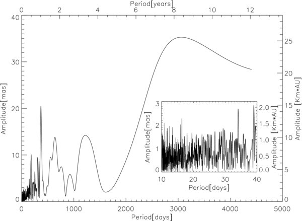
We have verified that these MDI radius data are not significantly contaminated by active regions as they rotate over the limb. Figure 5 shows the least-squares amplitude of the best-fit cosinusoid versus period over this long time series. The amplitude near one year period reflects the residual (uncorrected) satellite thermal signals also visible in the time series. The inset shows shorter period frequencies which include the rotational semi-period of about 14 days. The radius change amplitudes in this frequency range are about 1.5 mas and are not statistically significant. The absence of a 14 day signal gives us confidence that our global radius change measurements are not sensitive to active region contamination.
Figure 5. Best-fit least-squares amplitude (in units of milliarcsecond) vs. period from the radius change time series is plotted. The inset shows these results from shorter (rotational) timescales. The lack of a significant 14 day peak suggests that our radius results do not suffer from active region contamination.
Download figure:
Standard image High-resolution image
4. CONCLUSIONS
A complete solar cycle of satellite solar astrometry data has been analyzed to look for significant solar radius changes. Since these measurements are obtained from above the atmosphere and from a single long-running instrument, they are insensitive to atmospheric and many instrumental systematics. We find that the solar radius is constant to a high degree. Systematic changes in the solar radius that are synchronous/antisynchronous with the sunspot cycle must be smaller than 23 mas peak to peak. In addition, we find that the average solar size must not be changing by more than +1.2 mas yr−1 which is consistent with the Shapiro (1980) long-term planetary transit timing results. The pervasive difference between this observation of an effectively constant Sun and the ground-based solar astrometry that shows much larger apparent radius changes can only be accounted for by a changing terrestrial atmosphere (or errors in the measurements).