


ABSTRACT
First results from NASA's Interplanetary Boundary Explorer mission showed an unexpected "ribbon" of enhanced energetic neutral atom (ENA) flux spanning most of the sky. One explanation put forward suggests that the ribbon may be produced by secondary ENAs originating from pickup ions (PUIs) in the outer heliosheath (OHS). These PUIs are generated when primary ENAs born in the solar wind and inner heliosheath cross the heliopause and charge exchange in the nearby interstellar medium. One of the core assumptions underpinning this theory is that the newly born PUI ring is relatively stable with respect to wave generation, so that it can undergo charge exchange before becoming isotropized. We test this assumption using a linear kinetic theory and hybrid simulations of a low-density PUI ring interacting with instability-generated waves in a warm plasma of the OHS. It is shown that a broadband spectrum of waves is excited as a result of the cyclotron instability that efficiently scatters the ring ions. We also show that the ambient fluctuations in the OHS are unlikely to produce a measurable degree of resonant scattering of PUIs because their intensity is too low compared with the waves excited by the instability.
Export citation and abstract BibTeX RIS
1. INTRODUCTION
The Interplanetary Boundary Explorer (IBEX) satellite, launched in 2008 October, is currently observing the structure of the outer heliosphere in energetic neutral atoms (ENAs). The first year of operation brought forth a number of results that were not predicted by theoretical models (McComas et al. 2009; Fuselier et al. 2009; Funsten et al. 2009; Schwadron et al. 2009). The most striking discovery was a three-fold ENA enhancement measured at ∼1 keV above the surrounding emission (smaller at higher and lower energies) from a region in the sky in the shape of a nearly circular "ribbon." The largest intensity enhancement was measured at ∼1 keV (Fuselier et al. 2009).
Recently, Heerikhuisen et al. (2010) argued that the enhancement could be due to secondary ENAs produced in the outer heliosheath (OHS) from a parent population of heliosheath and solar wind pickup ions (PUIs). In their model, ENA emission comes primarily from those regions where the local interstellar (LISM) magnetic field is nearly perpendicular to the line of sight, i.e.,  (see also Schwadron et al. 2009). The model-predicted ribbon is consistent with both the ENA observations and the magnetic field orientation based on studies of the field draping around the heliopause (Pogorelov et al. 2009). The peak in intensity enhancement at 1 keV is explained by the fact that OHS PUIs produced from solar wind ENAs would have approximately that energy (1 keV corresponds to a proton speed of 438 km s−1).
One of the principal assumptions of the OHS PUI model of the ribbon is that the pitch-angle evolution of the ring ion distribution is slow enough to allow these particles to charge exchange (thus becoming secondary ENAs) before scattering completely onto a spherical shell. Heerikhuisen et al. (2010) used a "partial shell" distribution that is in between a narrow ring and an isotropic shell. The width of the ring was dependent on the angle between the parent ion velocity vector and LISM B implying, essentially, that scattering does not extend the velocity distribution to smaller pitch angles.
The time scale for charge exchange, τce = (nHσv)−1, where nH ≃ 0.2 cm−3 is the density of neutral H in the OHS, σ ≃ 2 × 10⁻¹⁵ cm2 is the charge-exchange cross section at 1 keV (Lindsay & Stebbings 2005), and v ∼ 400 km s−1 is the velocity of fast PUIs, is on the order of two years. This time is long compared with the electromagnetic time scales in the system that govern wave generation and pitch-angle scattering. The latter is typically some function of a gyro-period τg = 2π/Ωi (Ωi is the proton gyrofrequency) which is on the order of 4 minutes in the OHS. Thus, there is a factor of ∼105 disparity between temporal macroscales and microscales of the problem.
If waves are present in a plasma, a ring distribution will undergo pitch-angle scattering to become a shell (Williams & Zank 1994). Scattering will occur regardless of the origin of the waves, which could be part of ambient interstellar turbulence, generated near the heliopause, e.g., as a result of a large-scale instability (Axford et al. 1963; Fahr et al. 1986; Baranov et al. 1992), or excited by the PUI ring itself, which is known to be unstable to wave generation (Wu & Davidson 1972; Sharma & Patel 1986; Gary & Madland 1988). This paper deals primarily with PUI-excited waves. Below we investigate the process of wave excitation by a gyrating ion ring distribution in a warm plasma of the OHS using a linear Vlasov theory of electromagnetic fluctuations (Section 3) as well as nonlinear hybrid simulations of parallel (also called slab) modes in a plasma with thin and broadened ring-beams (Section 4). The latter approach allows us to examine self-consistently the scattering of PUIs on self-excited waves which leads, eventually, to their isotropization. We discuss the kinds of wave modes generated, the resulting spectrum of the waves, and the timescales for pitch-angle scattering. Finally, we compare the wave intensity generated as a result of the instability with possible ambient turbulence levels in the LISM (Section 5).
2. PUI DENSITIES IN THE OUTER HELIOSHEATH FROM IBEX ENA MEASUREMENTS
Using the published IBEX ENA intensities from the direction of the ribbon (Funsten et al. 2009; Heerikhuisen et al. 2010) we can estimate the parent population of PUIs produced by charge exchange of neutral solar wind atoms, which are presumably responsible for ENA emission at ∼1 keV. To do this, we note that in the limit of collisionless transport the ENA differential intensity at IBEX is an integral over the line of sight l,
where Δl is the width of the emitting region. According to MHD models (e.g., Pogorelov et al. 2009) the width of the OHS is on the order of 200 AU, which can be used for Δl above. The PUI differential intensity is fPUIp2, which for a ring distribution of thickness Δp in momentum and pitch-angle width ΔΩ may be approximated as

where nb is the number density of the PUI ring beam. With ΔΩ ∼ 2π, Δp = ΔE/v, where ΔE ∼ 0.5 keV (Figure 4 of Heerikhuisen et al. 2010), and JENA = 200 (cm2 s sr keV)−1 at 1 keV we obtain
Since the ambient plasma density in the OHS is about 0.08 cm−3 (Pogorelov et al. 2009), for all calculations in this paper we adopt a relative density of ring to background plasma ions of nb/ni = 1.8 × 10⁻⁴.
3. LINEAR VLASOV DISPERSION ANALYSIS
A warm Maxwellian electron–proton plasma supports three types of low-frequency waves propagating parallel to the LISM magnetic field B: an ion-acoustic longitudinal mode and two transverse electromagnetic waves (Alfvén-ion cyclotron and magnetosonic whistler). Relevant parameters are the plasma frequencies of the ions, assumed to be protons, and of the electrons, ωp, ωi, their cyclotron frequencies Ωp, Ωi, and their thermal speeds vti, vte. For particles of species α these are given by
where mα is the mass, eα is the signed electric charge, Tα is the temperature, and nα is the density of species α. Here we assume ni ≃ ne = 0.1 cm−3 and B = 2.5 μG, which are representative of the OHS region. With these parameters the Alfvén speed  km s−1 and the ion cyclotron frequency Ωi = 0.024 s−1.
The newly born PUIs represent an additional ring-beam component that is both drifting along B and gyrating in the perpendicular direction. We assume that the neutral solar wind hydrogen atoms are moving in a straight line radially from the Sun with a constant speed v = 400 km s−1. We work in the standard plasma frame with the z-axis directed along B. Upon ionization in a charge transfer collision with an interstellar proton the newly born PUI's velocity in this frame is vb = (v⊥bcos Ωbt, v⊥bsin Ωbt, v∥b), where v⊥b = vsin α, v∥b = vcos α, with α being the pickup angle (the angle between the direction of travel of the parent hydrogen atom and the mean magnetic field). Here we designate parameters pertaining to the PUI ring beam with the letter "b." The distribution function of the PUIs in the plasma frame is
The following analysis follows essentially that of Gary & Madland (1988), but using much lower ring-beam densities and background parameters appropriate for the OHS. We only consider parallel-propagating (slab) transverse electromagnetic waves because longitudinal electrostatic waves do not scatter ions in a pitch angle. For such modes the dispersion relation may be written as
where E is the electric field and the coefficients C and D are given by
where k is the parallel wavenumber, ω = ωr + iγ is the complex frequency, and Z is the plasma dispersion function. The normal modes of Equation (6) are given by C ± D = 0. Numerically found unstable roots are plotted in Figures 1 and 2 for Ti = Te = 0 and Ti = Te = 20, 000 K, respectively, the latter value is appropriate for the OHS plasma. The cold plasma case is included because it conveniently illustrates the physics of the instabilities and their coupling to the background plasma modes. We use three quasi-perpendicular pickup angles α = 80°, 85°, and 90°. Note that k = Ωi/Va corresponds to a wavelength of ∼5 × 108 cm.
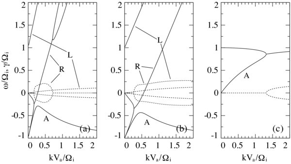
Figure 1. Cold plasma ring-beam instabilities for three pickup angles: α = 80° (a), α = 85° (b), and α = 90° (c). Solid lines show the real part of the complex frequency ωr, normalized to the ion cyclotron frequency, and dotted lines show the growth rate γ. The modes labeled "R" and "L" refer to the right- and the left-hand resonance, respectively. The mode labeled "A" is the Alfvén wave, modified by the instability. The magnetosonic wave is not shown and only positive k is used because of a space constraint.
Download figure:
Standard image High-resolution image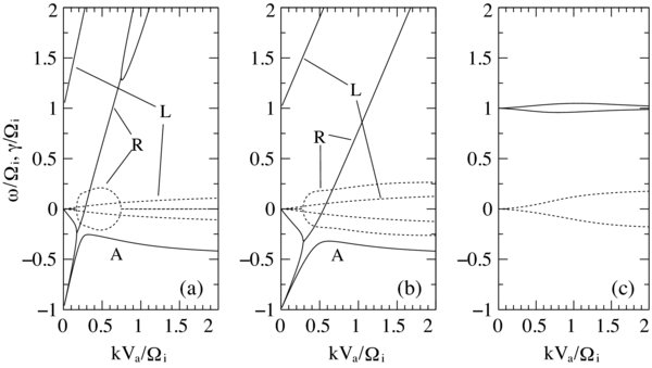
Figure 2. Same as Figure 1, but for a warm plasma in the OHS with Ti = Te = 20, 000 K.
Download figure:
Standard image High-resolution imageWith very low ring-beam densities (nb = 1.8 × 10⁻⁴ ni) instabilities arise only near resonance frequencies given by the zeroes of the denominators of the last two terms in Equations (7) and (8), i.e.,

There are several plasma beam instabilities known to operate in the low (near ion cyclotron) frequency regime (Gary et al. 1984; Winske et al. 1985). Of interest to us is the cyclotron resonant mode (Montgomery et al. 1976; Winske et al. 1984). The (mostly) right-hand part of this instability, labeled "R" in Figures 1(a) and 1(b), appears on the magnetosonic branch coupling it to the Alfvén wave, labeled "A" in that figure. This mode, corresponding to the minus sign in the resonance condition (9), can be either right-hand or left-hand polarized, with ωr > 0 and ωr < 0, respectively. The same dispersion branch features another instability at much higher (whistler) frequencies (Wu & Hartle 1974), which is of no interest here. The second instability corresponds to the plus in Equation (9) and is shown in the same figures as the "L" mode (Gary & Madland 1988). This left-hand instability generally has a smaller growth rate and is expected to be less important.
The "R" mode has regions of stability that move to higher wavenumbers with increased α, while the left-hand part is unstable for the entire range of pickup angles considered here. The low wavenumber stability region becomes an oppositely propagating magnetosonic wave (not shown). In the singular case α = 90°, the left- and the right-hand unstable branches merge together. From Figure 1(c) it can be seen that this instability modifies the parallel Alfvén dispersion branch, while the magnetosonic wave is not at all affected by the presence of the gyrating ring (Sharma & Patel 1986).
Dispersion curves in a warm plasma with a PUI beam are similar (Figure 2), except that the wave speeds are modified somewhat from the cold plasma case. Ti = 20, 000 K corresponds to a plasma β (the ratio of ion thermal to magnetic pressures) of 1.1. The Alfvén wave is strongly damped beyond Ωi/Va. At pickup angles close to 90° the right-hand mode becomes uncoupled from the Alfvén branch as seen in Figure 2(c). Apart from that the ion ring-beam instabilities in a warm heliosheath plasma have nearly identical growth rates owing to the resonant nature of the interaction. Typical growth rates are on the order of 0.2Ωi or 0.005 s−1.
4. HYBRID SIMULATIONS OF THE INSTABILITY AND PUI SCATTERING
The linear analysis predicts that waves will be excited, but reveals nothing about their behavior past the brief exponential growth phase. We certainly do not expect this phase to persist for more than a few gyroperiods because scattering will cause particles to spread in the pitch angle, leaving fewer and fewer to resonantly interact with each particular mode. While initially scattering will occur, we do not know yet whether it will lead to a complete isotropization of the ring, and if so, on what timescale. To proceed, a nonlinear model taking into account ion scattering must be used.
To investigate the excitation of slab (k||B) modes by the instability and track its nonlinear development and the scattering of freshly ionized PUI rings we use a one-dimensional (1D) hybrid electromagnetic code that treats ions as individual particles and electrons as a charge-neutralizing adiabatic fluid (e.g., Winske et al. 1984; Terasawa et al. 1986). The magnetic field is in the x-direction and the plasma is at rest initially (note the difference with Section 3, where B was in the z-direction). Grid resolution is uniform and equal to half the ion inertial length (0.5 c/ωi), which is sufficient to resolve the low-frequency electromagnetic modes. The simulation box length Lx is taken to be large enough to accommodate waves resonant with particles streaming along the field, i.e., Lx ≫ 2πv∥b/Ωi. A box size of ∼2000 c/ωi is sufficient to include the longest waves in the problem, excited by the particles with a zero pitch angle. We use equal numbers of particles (typically 25,000 per cell) for the background protons and for the ring beam. The latter are given a weight of nb/ne = 1.8 × 10⁻⁴, whereas the weight of the background ions is adjusted to 1 − nb/ne to maintain charge neutrality. These simulations have excellent statistics (∼2 × 10⁸ particles) ensuring that the weak PUI signal is easily identified against the background noise. Relevant dimensionless parameters are β = 1.1 and ωi/Ωi = c/Va = 1.74 × 10⁴. Periodic conditions are imposed at the spatial boundaries.
The first simulation starts with a narrow ring PUI distribution given by Equation (5) injected with vb = 450 km s−1 and α = 85°. Waves are excited from the thermal noise by the instability. These waves are initially counter-streaming with the beam and right-hand polarized, corresponding to the curve labeled "R" in Figure 2(b). Eventually, however, waves of both polarizations appear. Figure 3 shows several snapshots from the simulation at times t = 30/Ω−1i (1), t = 300/Ω−1i (2), and t = 4300/Ω−1i (3). The last panel corresponds to a real time of ∼2 days. The top panel for each time is the velocity distribution of the core (black) and the PUI ring (red), while the bottom panel shows the 1D power spectrum of the two transverse components of the magnetic field
where 〈 ⋅ ⋅ ⋅ 〉 denotes averaging with respect to x. In practice, a discrete Fourier transform of the two-point correlation function is taken (see Bieber et al. 1995). The spectrum above k = ωi/c is not part of the PUI signal, but is essentially white noise of numerical origin.
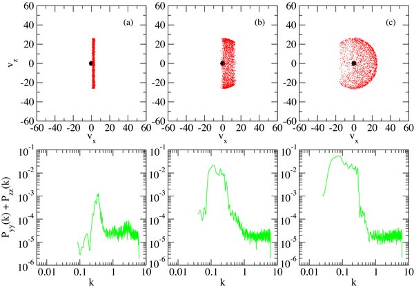
Figure 3. Top row: velocity distributions from the hybrid simulation of a thin ring (Equation (5)). Left panels (a) correspond to a time t = 30 Ω−1i = 0.35 hr into the simulation, middle panels (b) to t = 300 Ω−1i = 3.5 hr, and right panels (c) to t = 4300 Ω−1i = 50 hr since the start. Velocities are normalized to the Alfvén speed in the OHS Va = 17.2 km s−1. Core OHS protons are shown in black and PUIs are shown in red. Bottom row: power spectra in the two transverse components of the magnetic field. Wavenumber is measured in the units of ωi/c = 1.4 × 10⁻⁸ cm−1 and the power spectra are normalized to B2c/ωi = 0.045 G2 cm.
Download figure:
Standard image High-resolution imageThe narrow ring begins to broaden shortly after the start of the simulation. The waves initially form a narrowband spectrum centered at the resonant wavenumber k = (0.3–0.4) ωi/c (Figure 3(a)). As the simulation progresses particles scatter to smaller pitch angles filling the forward part of the shell and exciting progressively longer waves in the process. The spectral maximum shifts to k = (0.1–0.2) ωi/c (Figure 3(b)). Scattering across 90° is inhibited in this case in agreement with quasi-linear theory (e.g., Jokupii 1971). Some scattering is possible across the "resonance gap" due to a finite v/Va ≃ 0.038 (Schlickeiser 1989). After one day the PUI population is a nearly isotropic shell (Figure 3(c)). The wave spectrum is similar to t = 300 Ω−1i and extends down to k ≃ 0.03 ωi/c. A typical wave amplitude δB/B ∼ 0.05 near the end of the simulation. We note that the time scale for isotropization is almost 3 orders of magnitude larger than the characteristic timescale of the exponential wave growth phase (∼200 s).
Our second study case involves a broadened gyrotropic distribution of the form
(e.g., McClements & Dendy 1993), where v⊥b is the velocity spread of the PUIs in the OHS. Broadening in perpendicular velocity occurs because some of the parent ENAs were born in a fast SW, while others were produced in a slow wind or in the heliosheath. The distribution (11) is therefore a more realistic representation of the actual OHS PUI population.
In this simulation, we have used the same vb and α as in our narrow ring simulation, while the "thermal" spread of the distribution was half the mean speed v⊥t = 225 km s−1. Qualitatively, the results of this experiment, shown in Figure 4, are not very different from those obtained with a narrow ring. Both distributions have a similar number of wave-resonant particles (the resonance condition only depends on the parallel speed), which explains the similarity in the wave spectra in these two simulations. Note that in both cases the background ions, shown as black dots in Figures 3 and 4, were not affected by the low-density PUI ring.

Download figure:
Standard image High-resolution imageThe third simulation (Figure 5) shows a simulation for a widened distribution with an initial spread in the pitch angle. This is essentially the partial shell model of Heerikhuisen et al. (2010) and is given by
where θ is the pitch angle (cf. Equation (2)). A distribution of the form Equation (12) implies a range of pickup angles owing to (1) a difference in the direction of travel of parent heliosheath ENAs and (2) fluctuations in the direction of the magnetic field in the LISM. Here we used θ0 = 60° (cf. Section 2). While the initial distribution (12) resembles a partial shell attained after a scattering time of 3.5 hr in our earlier simulation (Figure 3(b)), this simulation is quite different because the partial shell is introduced without the associated turbulence. This leads to a scarcity of short waves in the spectrum.

Figure 5. Same as Figure 3, but for a widened PUI ring distribution given by Equation (12). The right panels correspond to t = 3000 Ω−1i = 35 hr since the start of the simulation.
Download figure:
Standard image High-resolution imageIn this scenario, short waves are not excited because the resonant particles are on a locally isotropic (stable) part of the shell. Only particles at the edge of the distribution (i.e., near θ0) generate the waves which explain the narrow spectrum in Figure 5(b). After some 35 hr (Figure 5(c)) the distribution has nearly relaxed to a spherical shell. Relaxation is faster in this case because there is no need for particles to scatter across 90°, as both hemispheres were equally populated by the PUIs from the start.
Selected pitch-angle distributions (PADs) of 1 keV PUI protons derived from the broad shell simulation at t = 3.5 hr and t ≃ 2 days are shown in Figure 6. PADs are constructed as phase angle averaged distributions per interval in velocity per interval in solid angle, namely, −ΔN/(2πv2ΔvΔμ), where μ is the pitch-angle cosine. At t = 3.5 hr (dashed line) the distribution is a partially filled shell with most particles traveling in the forward direction. The state at t = 50 hr consists essentially of two half shells (forward and backward) with little pitch-angle variation in each half shell. Despite some difficulty in scattering across μ = 0, particles do eventually migrate to the μ < 0 space with a final distribution invariably being an isotropic shell.

Figure 6. Phase-space density of PUIs, injected as a broad ring (Equation (11)), as a function of pitch-angle cosine μ at t = 3.5 hr (dashed line) and t = 50 hr (solid line). The units of the distribution function are arbitrary.
Download figure:
Standard image High-resolution image5. FLUCTUATION SPECTRA: INTERSTELLAR VERSUS LOCAL
The interstellar medium is known to be in a turbulent state from remote sensing measurements of electron density. The spectrum of the turbulence appears to be a power law with the Kolmogorov index −11/3, corresponding to a reduced 1D spectrum ∼k−5/3, spanning some 10 orders of magnitude in wavenumber from parsec scales down to 10−8 cm−1 (Armstrong et al. 1995). The power-law inertial range of the turbulence transitions to the energy containing range at the outer scale, where the energy input from large-scale motion of the interstellar gas occurs. Recent estimates place the outer scale at a few parsec, i.e., a few times 1018 cm (Haverkorn et al. 2008).
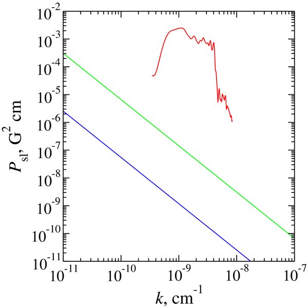
It is of interest to compare the ambient intensity of turbulent fluctuations at PUI resonant wavenumbers with the in situ turbulence generated by the ring instability. To perform this comparison we assume that the reduced (slab) LISM magnetic power spectrum is composed of a flat energy containing range followed by a Kolmogorov power law, i.e.,
where lc is the bendover length, which is related to the outer scale of the turbulence, and δB2sl is the mean square fluctuating field in the slab component. The spectrum (13) is normalized such that (cf. Equation (10))
We can also make a simple, but plausible, assumption that the turbulent magnetic field is a fixed fraction of the mean, i.e., that δB2/B2 ∼ 0.1–1. The slab component will be on average about a third of the total, so we may well take δB2sl/B2 ∼ 0.03–0.3. In addition to interstellar turbulence waves may be excited due to large-scale motions in the OHS. Some possible drivers include the solar wind large-scale transient structures and the solar-cycle dynamic pressure variations (Zank & Müller 2003; Scherer & Fahr 2003; Izmodenov et al. 2005), and the instability of the heliopause due to a difference in charge-exchange rates across the boundary (Liewer et al. 1996; Zank et al. 1996; Florinski et al. 2005; Borovikov et al. 2008). The scale of these motions is expected to be significantly shorter than the interstellar turbulent scales, perhaps on the order of 50 AU.
Figure 7 compares the LISM spectra in the slab component of the turbulence computed using B = 2.5 μG, lc = 1018 cm (blue line), the possible locally driven large-scale turbulence with lc = 7.5 × 1014 cm (green), and the wave intensity taken from the hybrid simulations in Figure 3(c) (red line). In deriving both ambient spectra we took δB2sl/B2 = 0.3, an extreme scenario which assumes LISM turbulence is very strong. Even so, the disparity in spatial scales combined with a steep power-law spectrum implies that the amount of fluctuations available to scatter PUIs is some 3–4 orders of magnitude below that of the self-excited waves. This means that ambient waves are not likely to contribute to the PUI scattering process. This conclusion remains in force for locally produced turbulence that is a result of a plasma motion on macroscopic scales, such as the Rayleigh–Taylor instability of the heliopause.
Figure 7. Comparison between the hypothetical LISM spectrum (blue), the large-scale locally driven turbulence (green), and the small-scale PUI instability-driven turbulence (red). The blue and green lines both have a slope of −5/3.
Download figure:
Standard image High-resolution image
6. DISCUSSION AND CONCLUSIONS
Independently using linear Vlasov theory and numerical hybrid simulations we have shown that a ring of pickup protons introduced into the OHS plasma by charge exchange with neutral solar wind hydrogen is unstable to wave generation by a resonant cyclotron mechanism. Hybrid simulations revealed that the generated waves in turn resonantly scatter the PUIs onto a shell. The time scale for isotropization is on the order of several days. This time, while significantly in excess of a proton gyroscale, is in turn substantially shorter than the time scale for charge exchange in the OHS, which is about two years. This appears to contradict the assumption of Heerikhuisen et al. (2010) that the PUI distribution remains narrow for an extended period of time. An anisotropic PUI distribution in the ribbon (i.e., the regions where  ) is required for their mechanism to work. While some isotropy will produce a ribbon, the flux levels will be considerably lower than what IBEX observes.
Waves generated by the PUI instability could contribute substantially to turbulence in the OHS region. The waves would persist even after the free energy in the ring has been exhausted because the damping rate of the long wave right-hand mode (i.e., the magnetosonic wave) is essentially zero in the OHS. The waves could eventually develop into a turbulent spectrum with implications for low-energy cosmic-ray scattering in the OHS (e.g., Florinski et al. 2003) and heating of the LISM plasma.
The simulations presented here were performed without taking into account spatial transport of PUIs. Particles with small pitch angles can potentially stream away from their place of origin along the interstellar magnetic field lines. Escape along field lines may alter the PUI distribution in the ENA emitting region (i.e., the ribbon). The emitting region cannot be very narrow, however, given that the width of the ribbon is about 20° (Fuselier et al. 2009), which corresponds to a width of some 100 AU in the OHS. It would take close to a year for 1 keV PUIs to travel that distance, which is again very long compared with the scale for the isotropization. We must conclude that spatial transport will not change our result appreciably except perhaps very close to the edge of the ribbon.
Our simulations were limited by the geometry of the wave field (slab only). An oblique multi-dimensional geometry could alter wave growth rates compared with the parallel case. This scenario is currently under investigation. The slab model is adequate for studying scattering in the pitch angle, but is not very suitable for spatial transport (especially, transport across the mean magnetic field) and turbulence development. Because wave growth is usually largest in the parallel direction, the slab model should provide a reasonable upper limit estimate on the wave generation process.
Our theoretical results are not the final verdict on the PUI ring stability in the OHS. On several occasions PUI rings injected at nearly perpendicular angles were observed to be stable, in seeming contradiction to the theoretical expectations. For example, Tsurutani et al. (1989) reported an absence of cyclotron waves near the comet Giacobini–Zinner when the pickup angle was between 70° and 90°. They also reported a lack of pitch-angle scattering and persistently high anisotropies of cometary PUIs. Gloeckler et al. (1995) showed that interstellar pickup H distributions measured at high heliographic latitudes (presumably for magnetic field directions close to radial) in the solar wind retained a relatively high anisotropy, which they interpreted as being due to a lack of instability-generated waves (see also Möbius et al. 1998). Finally, Oka et al. (2002) showed that He PUIs in some circumstances would have a torus-like distribution for a broad range of pickup angles. It appears that some physical effects that could delay isotropization are missing from existing theoretical models.
Turbulence cascading may be the missing piece of the puzzle. Our 1D simulations do not adequately describe this process, which is an essentially 3D effect, involving a transfer of power between oblique modes. The characteristic nonlinear time in the OHS is τnl ∼ 1/(kVa) ∼ 500 s, which is shorter than the isotropization time based on the results of Section 4. It is therefore possible that spectral transfer would channel the fluctuation power away from the resonant regime leaving fewer waves to scatter the PUIs. We will address this topic in the future using multi-dimensional electromagnetic plasma simulations (Khazanov & Singh 2008).
This research was supported, in part, by NASA grants NNX10AE46G and NNX09AG63G and by NSF grant AGS-0955700.