


ABSTRACT
This paper presents light curves as well as the first systematic characterization of variability of the 106 objects in the high-confidence Fermi Large Area Telescope Bright AGN Sample (LBAS). Weekly light curves of this sample, obtained during the first 11 months of the Fermi survey (2008 August 4–2009 July 4), are tested for variability and their properties are quantified through autocorrelation function and structure function analysis. For the brightest sources, 3 or 4 day binned light curves are extracted in order to determine power density spectra (PDSs) and to fit the temporal structure of major flares. More than 50% of the sources are found to be variable with high significance, where high states do not exceed 1/4 of the total observation range. Variation amplitudes are larger for flat spectrum radio quasars and low/intermediate synchrotron frequency peaked BL Lac objects. Autocorrelation timescales derived from weekly light curves vary from four to a dozen of weeks. Variable sources of the sample have weekly and 3–4 day bin light curves that can be described by 1/fα PDS, and show two kinds of gamma-ray variability: (1) rather constant baseline with sporadic flaring activity characterized by flatter PDS slopes resembling flickering and red noise with occasional intermittence and (2)—measured for a few blazars showing strong activity—complex and structured temporal profiles characterized by long-term memory and steeper PDS slopes, reflecting a random walk underlying mechanism. The average slope of the PDS of the brightest 22 FSRQs and of the 6 brightest BL Lacs is 1.5 and 1.7, respectively. The study of temporal profiles of well-resolved flares observed in the 10 brightest LBAS sources shows that they generally have symmetric profiles and that their total duration vary between 10 and 100 days. Results presented here can assist in source class recognition for unidentified sources and can serve as reference for more detailed analysis of the brightest gamma-ray blazars.
Export citation and abstract BibTeX RIS
1. INTRODUCTION
The high energy emission and the erratic, rapid and large-amplitude variability observed in all accessible spectral regimes (radio-to-gamma-ray) are two of the main defining properties of blazars (e.g., Ulrich et al. 1997; Webb 2006). The entire non-thermal continuum is believed to originate mainly in a relativistic jet, pointing close to our line of sight. Studies of variability in different spectral bands and correlations of multi-waveband variability patterns allow us to shed light on the physical processes in action in blazars, such as particle acceleration and emission mechanisms, relativistic beaming, origin of flares and size, structure, and location of the emission regions.
A proper understanding of the physical mechanisms responsible for variability is contingent upon a mathematical and statistical description of the phenomena. The study of variability is particularly important in gamma-ray astronomy. First, it assists in detecting faint sources, discriminating between real point sources and background fluctuations. Second, correlated multi-wavelength variability helps to recognize and identify the correct radio/optical/X-ray source counterparts within the gamma-ray position error box. A characterization of stand-alone gamma-ray variability for unidentified sources can also support the recognition of the correct source class (Nolan et al. 2003).
Even though it has already been studied for many years, the details of blazar variability in various bands have not yet been consistently compared against each other. A major contribution to our current understanding of the blazar phenomenon has been provided by EGRET, which discovered blazars as the largest class of identified and variable gamma-ray sources, in the band above 100 MeV. EGRET blazars showed variations on timescales from days to months (for the sources observed in several viewing periods) and gamma-ray flares on short timescales (1–3 days) have been detected in PKS 0528+134, 3C 279, PKS 1406 − 076, PKS 1633+382, PKS 1622 − 297, 3C 454.3 (see, e.g., von Montigny et al. 1995; Wallace et al. 2000; Nolan et al. 2003; Thompson 2006). In some cases, giant γ-ray outbursts were also found by EGRET (as for 3C 279; Hartman et al. 2001), and very rapid variability at very high energy was resolved (for example by HESS in PKS 2155 − 304; Aharonian et al. 2007). However, a complete characterization of the blazar gamma-ray variability was limited by statistics, number of the observations, and the EGRET pointed operating mode.
A new view on the gamma-ray variable sky is coming from the Fermi Large Area Telescope (LAT). Thanks to its large field of view (FOV; covering 20% of the sky at any instant and the full sky in about 3 hr), improved effective area and sensitivity, and the all-sky operating mode, the LAT is, therefore, an unprecedented instrument to monitor the variability emission of blazars in the energy band 20 MeV to >300 GeV (see, e.g., Atwood et al. 2009; Abdo et al. 2009a, 2010a). A major result obtained by the Fermi LAT during the first 3 months of observations was the publication of the Bright Source List (BSL; i.e., the 0FGL catalog; Abdo et al. 2009b), a list of 205 sources detected with a significance >10σ. Of these, 106 sources located at |b|>10° have been associated with high confidence with known active galactic nuclei (AGNs) and constitute the LAT Bright AGN sample (LBAS). The LBAS sample include two radio galaxies (Cen A and NGC 1275) and 104 blazars of which 58 are flat spectrum radio quasars (FSRQs), 42 are BL Lac objects, and 4 are blazars with uncertain classification (Abdo et al. 2009a).
This paper reports analysis results on the 11 month light curves of these 3 month selected bright AGNs, mostly blazars. Many of the light curves are, in fact, bright in the beginning of the considered 11 month period and then fade. This does not represent a particular bias, as also in the 11 month detected source catalog (Abdo et al. 2010a; first year LAT catalog, 1FGL) on average these sources are among the brightest blazars. A parallel and detailed study of spectral properties on the same LBAS sample is presented in Abdo et al. (2010b) while our analysis provides a temporal and flux variability analyses on the same sample. In Abdo et al. (2010b), the weekly gamma-ray spectral photon index is measured, in general, to vary in time only modestly (by <0.2–0.3) despite large variability of flux, and to vary only modestly within different blazar subclasses. In our paper, significant gamma-ray flux variability for about half of the LBAS objects is reported and for 1/4 of the sources, significant flares and outbursts are also found, showing a much stronger and violent variability of the flux than of the photon index.
In the following, we use a ΛCDM (concordance) cosmology with values given within 1σ of the Wilkinson Microwave Anisotropy Probe results (Komatsu et al. 2009), namely, Hubble constant value H0 = 71 km s−1 Mpc−1, Ωm = 0.27, ΩΛ = 0.73.
In Section 2, a description of the LAT observation and light curve extraction is reported, while in Section 3, results of variability search and amplitude quantification are presented. In Section 4, global variability properties of weekly bin light curves are presented through autocorrelation and structure function (SF) analysis. The analysis of the power spectral density and flare temporal profiles is presented in Sections 5 and 6, respectively, using finer sampling (3 and 4 day bins) light curves for the brightest sources. Summary and conclusions are given in Section 7. Cross-correlation studies between the γ-ray and other bands (such as radio-mm and optical bands), as well as more detailed studies on periodicity search, will be covered by other works based on the brightest sources where it is possible to obtain a finer-sampled flux light curves.
2. OBSERVATIONS WITH THE LAT AND LBAS LIGHT CURVES
The Fermi LAT (Atwood et al. 2009; Abdo et al. 2009d) is a pair-conversion gamma-ray telescope sensitive to photon energies greater than 20 MeV. It consists of a tracker (composed of two sections, front and back, with different capabilities), a calorimeter, and an anticoincidence system to reject the charged-particle background. The LAT has a large peak effective area (∼8000 cm2 for 1 GeV photons in the event class considered here), viewing ≃2.4 sr of the full sky with angular resolution (68% containment radius) better than ≃1° at E = 1 GeV.
Data used in this paper were collected during the first 11 months of the nominal all-sky survey, from 2008 August 4 to 2009 July 4 (Modified Julian Day (MJD) from 54682.655 to 55016.620).
In order to avoid background contamination from the bright Earth limb, time intervals where the Earth entered the LAT FOV were excluded from this study (corresponding to a rocking angle larger than 47°). In addition, events that were reconstructed within 8° of the Earth limb were excluded from the analysis (corresponding to a zenith angle cut of 105°). Due to uncertainties in the current calibration and the necessity of a trade-off between error accuracy and event statistics, only photons belonging to the "Diffuse" class and with energies above 100 MeV were retained. This event analysis was performed with the standard Fermi LAT ScienceTools software package59 (version v9r12) using in particular the tool gtlike, and using the first set of instrument response functions (IRFs) tuned with the flight data (P6_V3_DIFFUSE). In contrast to the preflight version, these IRFs take into account corrections for pile-up events. Since this is higher for lower energy photons, the measured photon index of a given source is about 0.1 higher (i.e., the spectrum is softer) with this IRF set as compared to the P6_V1_DIFFUSE one used previously in Abdo et al. (2009a, 2009b).
The light curves of all the LBAS sources were built using 7 day time intervals, for a total of 47 bins. For the brightest sources light curves were built using also time bins of 3 and 4 days (see Section 6). For each time bin, the flux, photon index, and test statistic (TS) of each source were determined, using the maximum-likelihood algorithm implemented in gtlike. The TS is defined as TS = 2Δlog(likelihood) between models with and without the source and it is a measure of the source significance (Mattox et al. 1996).
Photons were selected in a region of interest (RoI) 7° in radius centered on the position of the source of interest. In the RoI analysis, the sources were modeled as simple power law (F = dN/dE = N0E−p). The isotropic background (the sum of residual instrumental background and extragalactic diffuse gamma-ray background) was modeled with a simple power law. The GALPROP model version gll_iem_v01.fit (Strong et al. 2004a, 2004b) was used for the Galactic diffuse emission, with both flux and spectral photon index left free in the model fit. All errors reported in the figures or quoted in the text are 1σ statistical errors. The estimated systematic uncertainty on the flux is 10% at 100 MeV, 5% at 500 MeV, and 20% at 10 GeV.
For the 106 weekly light curves of LBAS sources analyzed in Sections 3 and 4, the flux in each time bin is reported for the energy band E > 300 MeV. This is the best band for reporting the flux because it is the band for which we have the highest signal to noise ratio for each source. The 3 day and 4 day bin light curves of the brightest sources analyzed in Sections 5 and 6 are extracted using the F(E > 100 MeV) flux.
3. VARIABILITY SEARCH AND AMPLITUDE IN WEEKLY LIGHT CURVES
The following variability analysis was performed using the weekly light curves reported in Figures 1 and 2. We used F(E > 300 MeV) (hereafter F300) in order to enable the comparison of the observed variability characteristics for the different sources.

Download figure:
Standard image High-resolution image
Download figure:
Standard image High-resolution image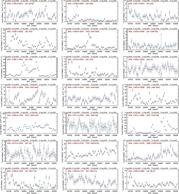
Download figure:
Standard image High-resolution image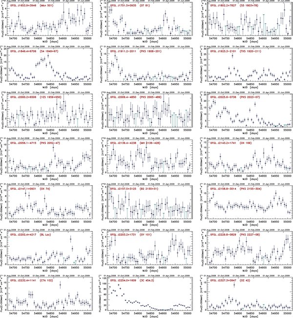
Figure 1. Light curves of the integrated flux (E > 300 MeV) measured in and averaged on weekly time bins obtained with the standard tool gtlike. In this figure, all the 84 LBAS objects that are selected for temporal variability study are reported. Filled circle symbols represent the best-fit values of the flux in the weekly bin with TS ⩾ 4 (approximatively 2σ), open circle symbols are the best-fit values of the flux in the bin with 1 < TS < 4, and the bars are the values of 1σ upper limits in the bin. Data in these plots are also available in Table 3 in the
Download figure:
Standard image High-resolution image
Figure 2. Twenty-two light curves that are excluded by the temporal analysis adopting the constraint of at least 60% of bins having a TS ⩾ 4 detection. Among these we note three peculiar light curves for the LSP blazars 0FGL J0531.0+1331, 0FGL J1719.3+1746, and 0FGL J2207.0 − 5347, showing strong flares and flux activity but only during a limited portion of the 11 months observed. Data appearing these plots are available in Table 3 in the
Download figure:
Standard image High-resolution imageBecause of the intrinsically variable nature of blazars for several sources we were not able to obtain a highly significant (TS ⩾ 25) estimate of the flux for all the 47 weeks. Therefore, in building the light curves we followed the same approach described in Abdo et al. (2009b) to preserve the maximum number of data points. For each time bin, we keep the best-fit value of the flux and its estimated error even when the source is below 5σ significance. Whenever TS ⩽ 1 we computed the 1σ upper limit and replaced the best-fit value of the flux with that upper limit. The weekly bin light curves extracted are presented in Figures 1 and 2, where filled circle symbols represent the best-fit values of the integrated flux (E > 300 MeV) in the weekly bin with TS ⩾ 4 (approximatively >2σ), open circle symbols are the best-fit values of the flux in the bin having 1 < TS < 4, and the bars are the values of 1σ upper limits in the bin.
We investigated whether a source had significant variations using a simple χ2 test,
where Fi are the F300 fluxes of each source on each bin and σi is the statistical uncertainty to which we added in quadrature σsyst = 0.03〈Fi〉 as an estimate of the systematic error (Abdo et al. 2009a, 2009d); Np is the number of points in each light curve having a TS ⩾ 4(∼2σ); and 〈Fi〉 is the unweighted mean of the flux. This test was applied to light curves containing only flux values with TS ⩾ 4 and excluding upper limits and fluxes with σi/Fi > 0.5 (see Figure 3). Figure 4 shows the distribution of the "coverage" fraction Np/Ntot, that is, the detection fraction of the total period of observation after this cut on the TS. The weekly light curves for the 84 LBAS objects for which this fraction is >60%, i.e., having at least 28 detections with TS ⩾ 4, are shown in Figure 1. The light curves of lower quality corresponding to the remaining 22 sources are shown in Figure 2.
Figure 3. Distribution of the relative flux errors  for all the 106 LBAS light curves and all the data points. The larger values of the relative error in the distribution labeled "All TS" are due to the counting of upper limits.
Download figure:
Standard image High-resolution image
Figure 4. Distribution of the coverage fraction Np/N of the observation period of each light curve.
Download figure:
Standard image High-resolution imageWe also quantify the variability amplitude of all the LBAS sources, using the "normalized excess variance" (Nandra et al. 1997; Edelson et al. 2002). This estimator is defined by
where S2 is the variance of the light curve and σ2err = σ2i + σ2sys. The error in σ2NXS was evaluated according to the prescription of Vaughan et al. (2003).
The results of this analysis are reported in Table 1: the first column lists the bright source list (0FGL list) name, Column 2 the other source name, and Column 3 the optical class. In the fourth column, we report the spectral energy distribution (SED) class, based on the peak frequency of the synchrotron component (νSp) of the broadband SED following the scheme outlined by Abdo et al. (2010c) which is an extension of the classification system introduced by Padovani & Giommi (1995) for BL Lacs. In this scheme we have: low synchrotron peaked (LSP; for νSpeak < 1014 Hz), intermediate synchrotron peaked (ISP; for 1014 Hz <νSpeak < 1015 Hz), and high synchrotron peaked (HSP; for νSpeak > 1015 Hz) blazars. Data listed in Columns 5–13 are the redshift, Np, the mean flux, the standard deviation of each light curve, the peak flux and error, the variability probability of χ2 (for Np − 1 degrees of freedom), and the normalized excess variance and error. Negative values of σ2NXS indicate absence or very small variability and/or slightly overestimated errors.
Table 1. Variability Indices and Amplitudes
| 0FGL | Other Name | Optical Class | SED Class | z | Np | 〈F300〉a | Sa | FMa | σMa | Prob | σ2NXS | err(σ2NXS) |
|---|---|---|---|---|---|---|---|---|---|---|---|---|
| J0017.4 − 0503 | PMN J0017 − 0512 | FSRQ | LSP | 0.227 | 24 | 2.30 | 1.37 | 5.65 | 1.07 | >99.0 | 0.24 | 0.08 |
| J0033.6 − 1921 | KUV 00311 − 1938 | BLLac | HSP | 0.610 | 31 | 1.12 | 0.52 | 2.80 | 1.04 | 12.0 | −0.09 | 0.08 |
| J0050.5 − 0928 | PKS 0048 − 097 | BLLac | ISP | >0.30 | 32 | 2.51 | 1.32 | 5.77 | 1.37 | >99.0 | 0.16 | 0.06 |
| J0051.1 − 0647 | PKS 0048 − 071 | FSRQ | LSP | 1.975 | 14 | 2.84 | 1.47 | 6.34 | 1.38 | >99.0 | 0.17 | 0.09 |
| J0112.1+2247 | S2 0109+22 | BLLac | ISP | >0.23 | 39 | 2.20 | 0.88 | 4.70 | 0.97 | 69.8 | 0.02 | 0.04 |
| J0118.7 − 2139 | PKS 0116 − 219 | FSRQ | LSP | 1.165 | 39 | 2.07 | 1.19 | 6.56 | 1.21 | >99.0 | 0.19 | 0.06 |
| J0120.5 − 2703 | PKS 0118 − 272 | BLLac | LSP | 0.557 | 34 | 1.52 | 0.55 | 2.89 | 0.91 | 1.8 | −0.11 | 0.06 |
| J0136.6+3903 | B3 0133+388 | BLLac | HSP | ... | 34 | 1.29 | 0.55 | 2.87 | 0.89 | 11.8 | −0.07 | 0.06 |
| J0137.1+4751 | DA 55 | FSRQ | LSP | 0.859 | 45 | 4.89 | 2.13 | 13.62 | 1.56 | >99.0 | 0.13 | 0.03 |
| J0144.5+2709 | TXS 0141+268 | BLLac | ISP | ... | 26 | 1.98 | 0.91 | 4.92 | 1.38 | 72.3 | 0.03 | 0.06 |
| J0145.1 − 2728 | PKS 0142 − 278 | FSRQ | LSP | 1.148 | 33 | 2.32 | 1.05 | 4.85 | 0.96 | >99.0 | 0.10 | 0.05 |
| J0204.8 − 1704 | PKS 0202 − 17 | FSRQ | LSP | 1.740 | 11 | 2.74 | 1.22 | 4.33 | 1.05 | >99.0 | 0.12 | 0.08 |
| J0210.8 − 5100 | PKS 0208 − 512 | FSRQ | LSP | 1.003 | 30 | 4.43 | 4.22 | 19.19 | 1.79 | >99.0 | 0.87 | 0.09 |
| J0217.8+0146 | OD 26 | FSRQ | LSP | 1.715 | 40 | 2.70 | 1.47 | 5.95 | 1.36 | >99.0 | 0.19 | 0.05 |
| J0220.9+3607 | S3 0218+35 | FSRQ | LSP | 0.944 | 42 | 3.55 | 1.71 | 8.98 | 1.37 | >99.0 | 0.15 | 0.04 |
| J0222.6+4302 | 3C 66A | BLLac | ISP | 0.444 | 47 | 7.92 | 5.05 | 34.06 | 2.52 | >99.0 | 0.38 | 0.03 |
| J0229.5 − 3640 | PKS 0227 − 369 | FSRQ | LSP | 2.115 | 20 | 2.62 | 1.45 | 6.30 | 1.18 | >99.0 | 0.22 | 0.07 |
| J0238.6+1636 | AO 0235+164 | BLLac | LSP | 0.940 | 44 | 13.19 | 10.73 | 40.78 | 2.42 | >99.0 | 0.66 | 0.03 |
| J0245.6 − 4656 | PKS 0244 − 470 | Un | ... | ... | 35 | 2.20 | 1.28 | 8.46 | 1.18 | >99.0 | 0.20 | 0.07 |
| J0303.7 − 2410 | PKS 0301 − 243 | BLLac | HSP | 0.260 | 36 | 1.95 | 0.78 | 4.78 | 1.19 | 43.3 | −0.01 | 0.04 |
| J0320.0+4131 | NGC 1275 | RG | ... | 0.018 | 46 | 6.54 | 2.42 | 12.30 | 1.71 | >99.0 | 0.09 | 0.02 |
| J0334.1 − 4006 | PKS 0332 − 403 | BLLac | LSP | ... | 44 | 1.98 | 0.72 | 4.36 | 1.16 | 15.1 | −0.04 | 0.04 |
| J0349.8 − 2102 | PKS 0347 − 211 | FSRQ | LSP | 2.944 | 33 | 2.86 | 1.51 | 7.00 | 1.55 | >99.0 | 0.18 | 0.05 |
| J0428.7 − 3755 | PKS 0426 − 380 | BLLac | LSP | 1.112 | 47 | 9.19 | 3.58 | 20.24 | 1.74 | >99.0 | 0.13 | 0.02 |
| J0449.7 − 4348 | PKS 0447 − 439 | BLLac | HSP | 0.205 | 47 | 3.40 | 1.44 | 8.79 | 1.55 | >99.0 | 0.09 | 0.03 |
| J0457.1 − 2325 | PKS 0454 − 234 | FSRQ | LSP | 1.003 | 47 | 13.56 | 6.78 | 34.39 | 2.23 | >99.0 | 0.24 | 0.02 |
| J0507.9+6739 | 1ES 0502+675 | BLLac | HSP | 0.416 | 23 | 1.14 | 0.50 | 2.63 | 0.85 | 6.3 | −0.14 | 0.10 |
| J0516.2 − 6200 | PKS 0516 − 621 | Un | ... | ... | 29 | 1.95 | 0.74 | 4.42 | 1.28 | 9.1 | −0.08 | 0.06 |
| J0531.0+1331 | PKS 0528+134 | FSRQ | LSP | 2.070 | 22 | 5.04 | 2.34 | 9.54 | 1.46 | >99.0 | 0.15 | 0.05 |
| J0538.8 − 4403 | PKS 0537 − 441 | BLLac | LSP | 0.892 | 47 | 9.23 | 3.58 | 17.65 | 2.06 | >99.0 | 0.13 | 0.02 |
| J0654.3+4513 | B3 0650+453 | FSRQ | LSP | 0.933 | 32 | 4.10 | 2.63 | 11.29 | 1.66 | >99.0 | 0.35 | 0.06 |
| J0654.3+5042 | GB6 J0654+5042 | Un | ... | ... | 28 | 2.00 | 0.94 | 3.89 | 1.06 | 91.4 | 0.06 | 0.06 |
| J0700.0 − 6611 | PKS 0700 − 661 | Un | ... | ... | 29 | 2.12 | 0.87 | 3.81 | 1.15 | 39.4 | −0.02 | 0.05 |
| J0712.9+5034 | GB6 J0712+5033 | BLLac | ISP | ... | 24 | 1.40 | 0.76 | 3.30 | 1.04 | 69.3 | 0.03 | 0.09 |
| J0714.2+1934 | MG2 J071354+1934 | FSRQ | LSP | 0.534 | 37 | 3.98 | 1.97 | 8.85 | 1.48 | >99.0 | 0.17 | 0.04 |
| J0719.4+3302 | B2 0716+33 | FSRQ | LSP | 0.779 | 37 | 2.78 | 1.59 | 7.26 | 1.11 | >99.0 | 0.23 | 0.06 |
| J0722.0+7120 | S5 0716+71 | BLLac | ISP | 0.310 | 45 | 4.94 | 2.63 | 11.56 | 1.44 | >99.0 | 0.24 | 0.03 |
| J0738.2+1738 | PKS 0735+17 | BLLac | LSP | 0.424 | 39 | 1.89 | 0.51 | 3.03 | 0.98 | 0.0 | −0.11 | 0.04 |
| J0818.3+4222 | OJ 425 | BLLac | LSP | 0.530 | 43 | 3.36 | 1.40 | 6.69 | 1.23 | >99.0 | 0.09 | 0.03 |
| J0824.9+5551 | TXS 0820+560 | FSRQ | LSP | 1.417 | 20 | 1.91 | 1.28 | 6.23 | 1.25 | >99.0 | 0.32 | 0.11 |
| J0855.4+2009 | OJ 287 | BLLac | LSP | 0.306 | 28 | 2.48 | 1.22 | 6.22 | 1.17 | >99.0 | 0.12 | 0.06 |
| J0921.2+4437 | S4 0917+44 | FSRQ | LSP | 2.190 | 44 | 6.56 | 4.32 | 19.52 | 1.70 | >99.0 | 0.41 | 0.04 |
| J0948.3+0019 | PMN J0948+0022 | FSRQ | LSP | 0.585 | 39 | 2.83 | 1.16 | 6.77 | 1.13 | >99.0 | 0.07 | 0.04 |
| J0957.6+5522 | 4C 55.17 | FSRQ | LSP | 0.896 | 47 | 3.55 | 0.76 | 5.05 | 1.07 | 2.1 | −0.03 | 0.02 |
| J1012.9+2435 | MG2 J101241+2439 | FSRQ | LSP | 1.805 | 28 | 2.11 | 0.93 | 4.09 | 0.98 | 71.7 | 0.02 | 0.05 |
| J1015.2+4927 | 1ES 1011+496 | BLLac | HSP | 0.212 | 47 | 2.40 | 0.79 | 4.74 | 1.12 | 36.4 | −0.01 | 0.03 |
| J1015.9+0515 | PMN J1016+0512 | FSRQ | LSP | 1.713 | 38 | 3.54 | 1.57 | 8.50 | 1.58 | >99.0 | 0.12 | 0.04 |
| J1034.0+6051 | S4 1030+61 | FSRQ | LSP | 1.401 | 24 | 2.00 | 0.74 | 4.44 | 1.01 | 52.4 | 0.00 | 0.04 |
| J1053.7+4926 | MS 1050.7+4946 | BLLac | ISP | 0.140 | 16 | 0.50 | 0.25 | 1.21 | 0.59 | 3.3 | −0.33 | 0.21 |
| J1054.5+2212 | 87GB 105148.6+222705 | BLLac | ISP | ... | 20 | 1.64 | 0.79 | 3.57 | 1.03 | 71.2 | 0.03 | 0.08 |
| J1057.8+0138 | 4C 01.28 | FSRQ | LSP | 0.888 | 44 | 3.50 | 1.62 | 6.77 | 1.21 | >99.0 | 0.12 | 0.04 |
| J1058.9+5629 | TXS 1055+567 | BLLac | ISP | 0.143 | 44 | 1.83 | 0.79 | 4.15 | 0.92 | 78.7 | 0.03 | 0.04 |
| J1100.2 − 8000 | PKS 1057 − 79 | BLLac | LSP | 0.569 | 18 | 2.69 | 0.86 | 4.84 | 1.42 | 9.2 | −0.08 | 0.06 |
| J1104.5+3811 | Mkn 421 | BLLac | HSP | 0.030 | 47 | 6.84 | 1.88 | 11.54 | 1.46 | >99.0 | 0.04 | 0.01 |
| J1129.8 − 1443 | PKS 1127 − 14 | FSRQ | LSP | 1.184 | 38 | 2.44 | 0.86 | 4.98 | 0.99 | 50.3 | 0.00 | 0.03 |
| J1146.7 − 3808 | PKS 1144 − 379 | FSRQ | LSP | 1.048 | 24 | 2.06 | 0.77 | 3.96 | 1.17 | 14.4 | −0.06 | 0.06 |
| J1159.2+2912 | 4C 29.45 | FSRQ | LSP | 0.729 | 43 | 3.06 | 1.14 | 6.68 | 1.17 | 98.1 | 0.05 | 0.03 |
| J1218.0+3006 | ON 325 | BLLac | HSP | 0.130 | 38 | 2.51 | 2.51 | 15.11 | 1.82 | >99.0 | 0.90 | 0.12 |
| J1221.7+2814 | W Com | BLLac | ISP | 0.102 | 43 | 2.58 | 1.27 | 6.86 | 1.44 | >99.0 | 0.12 | 0.05 |
| J1229.1+0202 | 3C 273 | FSRQ | LSP | 0.158 | 47 | 8.68 | 5.47 | 23.11 | 2.07 | >99.0 | 0.38 | 0.03 |
| J1246.6 − 2544 | PKS 1244 − 255 | FSRQ | LSP | 0.635 | 37 | 4.60 | 3.81 | 18.28 | 1.75 | >99.0 | 0.64 | 0.07 |
| J1253.4+5300 | S4 1250+53 | BLLac | LSP | ... | 29 | 1.45 | 0.47 | 2.93 | 0.89 | 0.9 | −0.12 | 0.06 |
| J1256.1 − 0548 | 3C 279 | FSRQ | LSP | 0.536 | 47 | 15.69 | 12.31 | 50.91 | 2.61 | >99.0 | 0.62 | 0.03 |
| J1310.6+3220 | OP 313 | FSRQ | LSP | 0.997 | 41 | 3.38 | 2.31 | 11.50 | 1.39 | >99.0 | 0.40 | 0.06 |
| J1325.4 − 4303 | Cen A | RG | ... | 0.002 | 44 | 3.41 | 0.82 | 5.71 | 1.20 | 0.8 | −0.05 | 0.02 |
| J1331.7 − 0506 | PKS 1329 − 049 | FSRQ | LSP | 2.150 | 39 | 3.86 | 1.86 | 7.88 | 1.20 | >99.0 | 0.16 | 0.04 |
| J1333.3+5058 | 87GB 133151.1+511313 | FSRQ | LSP | 1.362 | 20 | 1.72 | 0.53 | 3.18 | 0.89 | 4.8 | −0.09 | 0.06 |
| J1355.0 − 1044 | PKS 1352 − 104 | FSRQ | LSP | 0.330 | 13 | 2.92 | 1.76 | 7.38 | 1.45 | >99.0 | 0.27 | 0.11 |
| J1427.1+2347 | PKS 1424+240 | BLLac | ISP | ... | 45 | 2.91 | 1.08 | 6.73 | 1.47 | 94.0 | 0.04 | 0.03 |
| J1457.6 − 3538 | PKS 1454 − 354 | FSRQ | LSP | 1.424 | 46 | 8.49 | 5.16 | 24.30 | 2.08 | >99.0 | 0.34 | 0.03 |
| J1504.4+1030 | PKS 1502+106 | FSRQ | LSP | 1.839 | 47 | 29.57 | 12.15 | 78.44 | 3.79 | >99.0 | 0.17 | 0.01 |
| J1511.2 − 0536 | PKS 1508 − 05 | FSRQ | LSP | 1.185 | 31 | 2.17 | 0.58 | 3.56 | 0.99 | 0.0 | −0.14 | 0.05 |
| J1512.7 − 0905 | PKS 1510 − 08 | FSRQ | LSP | 0.360 | 47 | 28.67 | 27.21 | 115.94 | 3.82 | >99.0 | 0.91 | 0.02 |
| J1517.9 − 2423 | AP Lib | BLLac | LSP | 0.048 | 35 | 2.62 | 0.76 | 4.65 | 1.24 | 0.5 | −0.09 | 0.04 |
| J1522.2+3143 | TXS 1520+319 | FSRQ | LSP | 1.487 | 47 | 8.88 | 3.01 | 17.53 | 1.69 | >99.0 | 0.09 | 0.01 |
| J1543.1+6130 | GB6 J1542+6129 | BLLac | ISP | ... | 39 | 2.39 | 1.26 | 5.93 | 1.03 | >99.0 | 0.16 | 0.05 |
| J1553.4+1255 | S3 1551+13 | FSRQ | LSP | 1.308 | 32 | 3.92 | 2.13 | 9.14 | 1.57 | >99.0 | 0.22 | 0.05 |
| J1555.8+1110 | PG 1553+11 | BLLac | HSP | >0.09 | 44 | 3.31 | 1.12 | 6.05 | 1.21 | 93.2 | 0.03 | 0.02 |
| J1625.8 − 2527 | PKS 1622 − 253 | FSRQ | LSP | 0.786 | 26 | 3.90 | 1.20 | 7.21 | 2.00 | 3.3 | −0.08 | 0.05 |
| J1635.2+3809 | 4C 38.41 | FSRQ | LSP | 1.814 | 47 | 4.09 | 2.06 | 12.32 | 1.34 | >99.0 | 0.19 | 0.04 |
| J1653.9+3946 | Mkn 501 | BLLac | HSP | 0.033 | 42 | 2.61 | 1.27 | 5.67 | 1.23 | >99.0 | 0.12 | 0.05 |
| J1719.3+1746 | S3 1717+17 | BLLac | LSP | 0.137 | 18 | 3.04 | 2.18 | 9.40 | 1.61 | >99.0 | 0.44 | 0.11 |
| J1751.5+0935 | OT 81 | BLLac | LSP | 0.322 | 33 | 3.96 | 2.72 | 10.82 | 1.73 | >99.0 | 0.38 | 0.07 |
| J1802.2+7827 | S5 1803+78 | BLLac | LSP | 0.680 | 30 | 1.94 | 0.85 | 4.04 | 1.05 | 77.3 | 0.03 | 0.05 |
| J1847.8+3223 | B2 1846+32A | FSRQ | LSP | 0.798 | 24 | 3.30 | 1.67 | 6.85 | 1.23 | >99.0 | 0.17 | 0.06 |
| J1849.4+6706 | S4 1849+67 | FSRQ | LSP | 0.657 | 46 | 6.31 | 4.99 | 19.62 | 1.86 | >99.0 | 0.60 | 0.05 |
| J1911.2 − 2011 | PKS 1908 − 201 | FSRQ | LSP | 1.119 | 31 | 4.35 | 3.01 | 13.95 | 1.77 | >99.0 | 0.40 | 0.07 |
| J1923.3 − 2101 | TXS 1920 − 211 | FSRQ | LSP | 0.874 | 41 | 6.18 | 3.86 | 23.52 | 2.25 | >99.0 | 0.34 | 0.04 |
| J2000.2+6506 | 1ES 1959+650 | BLLac | HSP | 0.047 | 43 | 2.70 | 1.19 | 5.80 | 2.32 | 94.8 | 0.05 | 0.04 |
| J2009.4 − 4850 | PKS 2005 − 489 | BLLac | HSP | 0.071 | 30 | 1.96 | 0.62 | 3.53 | 1.71 | 1.0 | −0.11 | 0.05 |
| J2025.6 − 0736 | PKS 2023 − 07 | FSRQ | LSP | 1.388 | 40 | 7.60 | 5.07 | 19.39 | 1.85 | >99.0 | 0.42 | 0.04 |
| J2056.1 − 4715 | PKS 2052 − 47 | FSRQ | LSP | 1.491 | 37 | 3.41 | 1.66 | 8.96 | 1.41 | >99.0 | 0.15 | 0.04 |
| J2139.4 − 4238 | MH 2136 − 428 | BLLac | ISP | >0.24 | 45 | 2.71 | 1.18 | 5.60 | 1.34 | 98.4 | 0.06 | 0.04 |
| J2143.2+1741 | OX 169 | FSRQ | LSP | 0.213 | 41 | 3.75 | 1.87 | 9.95 | 1.47 | >99.0 | 0.17 | 0.04 |
| J2147.1+0931 | OX 74 | FSRQ | LSP | 1.113 | 45 | 3.32 | 1.66 | 8.93 | 1.18 | >99.0 | 0.17 | 0.04 |
| J2157.5+3125 | B2 2155+31 | FSRQ | LSP | 1.486 | 28 | 2.12 | 0.72 | 4.01 | 1.01 | 8.4 | −0.06 | 0.05 |
| J2158.8 − 3014 | PKS 2155 − 304 | BLLac | HSP | 0.116 | 47 | 7.89 | 2.38 | 14.93 | 1.75 | >99.0 | 0.06 | 0.01 |
| J2202.4+4217 | BL Lac | BLLac | LSP | 0.069 | 42 | 4.26 | 2.31 | 13.90 | 1.90 | >99.0 | 0.22 | 0.04 |
| J2203.2+1731 | OY 101 | FSRQ | LSP | 1.076 | 34 | 2.83 | 1.29 | 5.49 | 1.28 | >99.0 | 0.10 | 0.05 |
| J2207.0 − 5347 | PKS 2204 − 54 | FSRQ | LSP | 1.215 | 11 | 2.44 | 2.65 | 10.71 | 1.40 | >99.0 | 1.17 | 0.24 |
| J2229.8 − 0829 | PKS 2227 − 08 | FSRQ | LSP | 1.560 | 41 | 3.71 | 1.40 | 7.05 | 1.16 | >99.0 | 0.07 | 0.03 |
| J2232.4+1141 | CTA 102 | FSRQ | LSP | 1.037 | 43 | 3.10 | 1.50 | 9.11 | 1.34 | >99.0 | 0.15 | 0.04 |
| J2254.0+1609 | 3C 454.3 | FSRQ | LSP | 0.859 | 46 | 27.36 | 24.58 | 94.73 | 3.91 | >99.0 | 0.82 | 0.02 |
| J2325.3+3959 | B3 2322+396 | BLLac | LSP | ... | 20 | 2.07 | 1.33 | 5.32 | 1.34 | >99.0 | 0.26 | 0.11 |
| J2327.3+0947 | OZ 42 | FSRQ | LSP | 1.843 | 42 | 3.05 | 2.12 | 13.67 | 1.39 | >99.0 | 0.40 | 0.06 |
| J2345.5 − 1559 | PMN J2345 − 1555 | FSRQ | LSP | 0.621 | 19 | 2.29 | 0.93 | 4.47 | 1.03 | 69.3 | 0.02 | 0.06 |
The large majority of sources (74) belong to the LSP class, which includes all FSRQs (58) and several BL Lacs (16), while both ISP and HSP classes have each 13 BL Lacs sources. There are also two radio galaxies (NGC 1275 also known as Per A and Cen A) and four objects which cannot be well classified for paucity of data.
On the basis of the χ2 test, variability was detected in 68 out of the 106 LBAS sources with a significance higher than 99% (Column 11 in Table 1). Note, however, that as demonstrated by Figure 19 in Abdo et al. (2010e) the χ2 has a strong dependence on the statistical flux uncertainties. For the fainter sources this leads to a reduction of the χ2 for a given fractional flux variation and then a source can be considered significantly variable only if it is both intrinsically variable and sufficiently bright. Therefore, fainter sources can appear less variable than brighter sources simply because we cannot measure their variability.
In Abdo et al. (2009a), 56 sources were flagged as variable based on the results of a χ2 test applied to weekly light curves covering the first 3 months of operation. To compare our results with those reported in Abdo et al. (2009a), we divided the light curves in four consecutive segments having a duration of about 12 weeks, and the χ2 test was applied to each of them. Forty two sources were found variable with a significance higher than 99% during the first light curve segment (corresponding to about the same time interval analyzed in Abdo et al. 2009a, 2009b; 28 in the second, 23 in the third, and 19 in the last). The difference in the number of variable sources in the first segment with respect to Abdo et al. (2009a) results can be explained by taking into account that in Abdo et al. (2009a) all light curve data points, including those with TS < 4, were considered in the calculation of the χ2 and the likelihood analysis was performed with a different combination of IRFs and diffuse models. The decreasing number of variable sources revealed in the four time intervals is a selection effect. We are using the BSL sample, so there are disproportionately more objects which happened to flare up at the beginning of the interval and then faded. However, this is illustrative of one of the distinctive aspects of the intrinsic characteristics of the blazars' variability: alternate periods of flaring and low activity states. However, the total period of our observations is in most cases still too short to allow an estimation of the duty cycle of the blazar variability in the gamma-ray energy range. Flux distributions can be used to characterize the gamma-ray duty cycle, and for two FSRQs (3C 454.3 and PKS 1510 − 08) that were very active during the first 1.5 years of LAT observations, the fluxes are found distributed in a different way with respect to a lognormal distribution (Tavecchio et al. 2010).
Figure 5 shows the distribution of the peak (FM) values for LSP, ISP, and HSP. It can be noted that only a few LSP were detected in exceptionally bright states with a flux FM > 2 × 10⁻⁷ photon cm-2 s−1.

Figure 5. Distribution of FM for the LSP, ISP, and HSP light curves with a coverage factor Np/N⩾ 60%.
Download figure:
Standard image High-resolution imageFigures 6 and 7 show the distributions of σ2NXS and of the ratio between the highest measured flux to the mean FM/〈F〉 for the above three SED classes. These figures were obtained using only the 84 light curves with a coverage of Np/Ntot ⩾ 60%. Variability amplitude of LSPs is generally larger than for ISPs and HSPs with the remarkable exception of the HSP source 0FGL J1218.0+3006 (ON 325, also known as Ton 605) which has the higher values of FM/〈F〉 among the LBAS sources (see also lower panel of Figure 9 for the maximum ratio of consecutive weekly flux values). This source was always close to the detection limit on a week timescale, but a strong flare was observed during 2009 October 10–15. This shows that although HSP seems to have, on average, a variability amplitude smaller than those observed in LSP, episodic large flaring activity can also be observed for this subclass of blazars.
Figure 6. Distribution of the excess variance for the LSP, ISP, and HSP light curves with a coverage factor of Np/N ⩾ 60%.
Download figure:
Standard image High-resolution image
Figure 7. Distribution of FM/〈F〉 for the LSP, ISP, and HSP light curves with a coverage factor of Np/N ⩾ 60%.
Download figure:
Standard image High-resolution imageAmong the sources with a coverage <60% (22 sources), three sources have FM ∼ 10−7 photon cm-2 s−1. 0FGL J2207.0 − 5347 (PKS 2204 − 54) has a light curve dominated by a short and intense flare detected during 2008 September 3–8; 0FGL J1719.3+1746 (PKS 1717+177) was mainly active during 2008 September; 0FGL J0531.0+1331 (PKS 0528+134), one of the most active source during the EGRET era, was in a relative bright state during 2008 September–November, with two flaring episodes, it then decreased to a flux close to the Fermi LAT detection threshold on a week timescale.
To obtain an estimate of the time spent by each source in a bright state we evaluate the number of time bins (Nb) for which (Fi − σi)>(〈F〉 + 1.5 × S). The distribution of the ratio Nb/N in percent is reported in Figure 8. We see that high states exceeding one-fourth of the duration of the entire observation window are absent and that a very high number of sources were bright over a time interval shorter than the 5% of the total observation time. This distribution can be approximately described by a power law (NS = (382 ± 107) × (100Nb/N)−1.9 ± 0.2).
Figure 8. Distribution of Nb/N. This distribution could be described by a power law: NS = (382 ± 107) × (100Nb/N)−1.9 ± 0.2.
Download figure:
Standard image High-resolution image4. CHARACTERIZATION OF TEMPORAL VARIABILITY IN WEEKLY LIGHT CURVES
For the first time Fermi LAT is enabling a long-term view of high-energy source variability on a uniformly selected sample of gamma-ray sources. In this section, we report the first and quantitative outlook to the 11 month weekly light curves shown in the previous section. As mentioned previously, 84 of the LBAS sources have at least 60% of the 47 weekly bins (at least 28 weekly bins) with TS ⩾ 4 flux detections (filled points in Figure 1). This allowed a quantitative time series analysis along the entire light curve (global analyses such as PDS or autocorrelation that are distinct from local analysis such as the flare shape analysis reported in Section 6, or wavelet analysis). In particular, the discrete auto correlation function (DACF) and the first-order SF are suitable methods to provide these first insights into fluctuation modes and characteristic timescales. To reduce contamination in results caused by the low brightness and non-variable sources that provide a white-noise contribution, a sub-sample of the 56 brightest and most variable objects is extracted from this list based on variability probability of χ2 greater than 99% and normalized excess variance σ2NXS ⩾ 0.09 (with exception of Mkn 421, 0FGL J1104.5+3811, and PKS 2155 − 304, 0FGL J2158.8 − 3014, taken into account because of their persisting level of flux over the entire period: see Figure 1, respectively, and Table 1).
In the upper panel of Figure 9, the scatter plot of the observed maximum of subsequent weekly flux variations versus the redshift (known for 53 of the 56 brightest and variable sources selected) is represented, for a comparison with the variable blazars seen during the EGRET era. The brightest blazars also showing the most apparent violent variations on weekly timescales, during these first 11 months of Fermi survey, are FSRQs PKS 1510 − 08 (Marscher et al. 2010; Abdo et al. 2010i), PKS 1502+106 (Abdo et al. 2010d), 3C 454.3 (Abdo et al. 2009c), 3C 279 (Abdo et al. 2010g), PKS 0454 − 234, and an ISP BL Lac object, 3C 66A. In a few cases, other sources historically classified as BL Lac objects showed rather violent gamma-ray variations, such as AO 0235+164 and BL Lacertae where flux increases approximatively around or above 10−7 photon cm−2 s−1at E > 300 MeV.

Figure 9. Upper panel: scatter plot of the observed maximum of flux variations (Fhigh/Flow) in adjacent weekly bins (variations for both flux increases or decreases in subsequent weeks) vs. the redshift for the 53 brightest and most variable sources of Table 1 with known z (or lower limit) and coverage Nb/N ⩾ 60%. Most scattered sources are labeled, and different symbols and colors are used according to the classification of Table 1. Lower panel: scatter plot of the maximum ratio of flux variations in adjacent weekly bins vs. the redshift for the same sources. A possible separation band between BL Lac objects and FSRQs is indicated by the line.
Download figure:
Standard image High-resolution imageIn the lower panel of Figure 9, the observed maximum of the ratio of weekly flux values Fhigh/Flow in subsequent time bins (Fhigh being the highest value in a pair of subsequent values both in case of increasing or decreasing trend) is plotted against the redshift. This plot points out a possible separation band between BL Lac objects and FSRQs. The transition region between the two families is roughly placed between redshift 0.5 and 1. In agreement with the results of Section 3 and the spectral results reported in Abdo et al. (2010b), the HSP BL Lac objects are well separated, being at the lowest redshift and least variable sources (with the exception of ON 325 as mentioned in the previous section). This ratio, being the relative flux change in subsequent weeks, is rather independent of redshift and more directly related to intrinsic dynamics, also points out different blazars as intrinsically violent variable sources, such as DA 55, B2 0716+33, OP 313, PKS 1454 − 354, and PKS 1329 − 049 (FSRQs), and also BL Lac objects such as ON 325 and W Com. This scatter plot shows that variability and redshift for AO 0235+164 fall into the FSRQs region, as confirmed by the physical properties of this source, more similar to that of an FSRQs than to that of a BL Lac.
The analysis of the DACF and SF techniques is applied to this same sample of the LBAS list. The DACF allows us to also investigate the level of autocorrelation in discrete data sets (see, e.g., Edelson & Krolik 1988; Hufnagel & Bregman 1992) without any interpolation and any invention of artificial data points. The pairs [F(ti), F(tj)] of a discrete data set are first combined in unbinned discrete correlations
where 〈F〉 is the average values of the sample and σF is the standard deviation. Each of these correlations is associated with the pairwise lag Δtij = tj − ti and every value represents information about real points. The DACF is obtained by binning the C(u)ij in time for each lag Δt, and averaging over the number M of pairs whose time lag Δtij is inside Δt:
The choice of the bin size for irregular time series is governed by the trade-off between the desired accuracy in the mean calculation and the desired resolution in the description of the correlation curve. In this analysis, the bin is chosen equal to the sampling, 1 week, because of the limited temporal range and regularity (no gaps) of the light curves.
The SF is equivalent to the power density spectrum (PDS) of the signal calculated in the time domain instead of frequency space, which makes it less subject to sampling problems in the presence of very irregular time series, such as windowing and aliasing (see, e.g., Simonetti et al. 1985; Smith et al. 1993; Lainela & Valtaoja 1993; Paltani et al. 1997). This function represents merely a measure of the mean squared of the flux differences at times t and t + Δt of N pairs with the same time separation Δt, along the whole time series. The first-order SF is defined as
where Fi is the discrete signal at time t. The general definition involves an ensemble average. This function is a sort of a "running" variance of the process that is able to discern the range of timescales that contribute to variations in the time series.
In the DACF and SF analysis of these 56 weekly LBAS light curves, true upper limits (TS < 1) are conservatively considered as values close to zero (i.e., 10−12 photon cm-2 s−1, well below the 11 month LAT sensitivity), avoiding in this way the bias of an underestimation of low flux states that a replacement with empty gaps of such bins would cause. The SF analysis performed on light curves, taking into account upper limits as explained above and, as a test, applied again on the same light curves with upper limits replaced by empty gaps, demonstrates a very low difference in results (about 80% of the sources show a difference in the calculated SF power-law index of ±0.05).
Examples of 12 DACF and SF functions applied to these weekly light curves are reported in Figure 10. They show different autocorrelation patterns, and different central peak amplitude, and different temporal trends and slopes in logarithmic SF representation, pointing out different variability modes and timescales. The time lag Δtcross where the DACF value crosses zero for the first time can indicate the maximum correlation scale, while equally spaced and repeated peaks in the function shape can point out characteristic timescales and hints for possible periodicity. Deep drops of the SF value can mean a small variance and provide again possible signature for a characteristic timescale. The ideal SF increases with the lag Δt in a log–log representation as in the plots shown in Figure 10. PDSs of blazars' light curves usually show power-law dependence on the signal temporal frequency f in a wide range of frequencies (P(f) ∝ 1/fα). In case of sufficient sampling, sufficient total time range, and low noise, the SF can show a steep linear trend in a certain range of lags in logarithmic scale with index simply related to the PDS power index by S ∝ (Δt)α−1 (Hughes et al. 1992; Lainela & Valtaoja 1993). If a maximum correlation timescale is reached in a light curve, the SF is constant for longer lags, and such a turnover point between the power-law portion and the constant trend can identify another important characteristic timescale. In real cases, the identification of a firm break in the SF and the fit of the trend is difficult and misleading because spurious features are common in these functions, resulting in a wiggling pattern and artificial breaks. These spurious features are systematic effects resulting from the finite length of the light curves, together with the random nature of the variability process itself (Emmanoulopoulos et al. 2010).

Figure 10. Example of DACF and SF functions applied to the weekly light curves of 12 LBAS blazars (from the left to bottom right: 3C 66A, AO 0235+164, PKS 0426 − 380, S5 0716+71, S4 0917+44, Mkn 421, 3C 273, 3C 279, 4C 38.41, S4 1849+67, TXS 1920+211, and 3C 454.3). They show different autocorrelation patterns, different zero lag peak amplitudes and crossing times, and different temporal power spectral trends and slopes, pointing out more different variability modes.
Download figure:
Standard image High-resolution imageIn Figure 11, we show four distributions of the power indices α evaluated through the SF applied in a blind mode to each of the 56 selected light curves from the minimum lag Δtmin of 1 week to a maximum lag Δtmax of 1/3, 1/2, 2/3, and 4/5 of the total time range I(=tmax − tmin). Most of the α values are distributed between 1.1 and 1.6, meaning a fluctuation mode about halfway between the pure flickering (also known as red noise, α = 1) and the pure shot noise (also known as brown noise or Brownian variability, α = 2, typically produced by a random walk process). Weaker sources, more affected by error dispersion, cause a whitening of the variability and shift the distributions closer to flickering, as well as the blind application of the SF when the maximum lag adopted is above the function break. For example, for the weekly light curve of 3C 279 the power index α estimated by the average of the four blind SF runs is 1.25, whiter than the value found when adopting Δtmax = (1/3)I only (well below the break) where we have a value of about 1.6 (Figure 11, top panel), in agreement with the value for the 3 day bin light curve found with the direct calculation of PDS analysis (Section 5).

Figure 11. Distributions of the PDS power indices α for the weekly light curves of the 56 most bright and variable LBAS sources, selected as explained in the text. The values are obtained applying the SF considering four maximum lags (1/3, 1/2, top panel, and 2/3 and 4/5 bottom panel, of the total time range I = tmax − tmin). These distributions are peaked for values of the power index between 1.1 and 1.6.
Download figure:
Standard image High-resolution imageThese blind SF results at mid and long-term timescales appear roughly in agreement with the observed long-term optical variability based on some samples (for example optical spectral slope in the range 1.3–1.8 in Heidt & Wagner 1996; Webb & Malkan 2000; Fiorucci et al. 2003; Ciprini et al. 2007), and short-term X-ray variability (e.g., Green et al. 1993; Lawrence & Papadakis 1993; McHardy 2008). Radio light curves have power spectra with slopes around 2 in timescales from days up to several years (e.g., Hufnagel & Bregman 1992; Hughes et al. 1992; Lainela & Valtaoja 1993; Aller et al. 1999; Ciaramella et al. 2004; Hovatta et al. 2007; Nieppola et al. 2009).
The cases of 3C 454.3 (0FGL J2254.0+1609 a typical FSRQ) and AO 0235+164 (0FGL J0238.6+1636, LSP BL Lac object) are remarkable, showing, with weekly bin resolution, a full Brownian (α ≳ 1.8) γ-ray variability with main monotonic baseline trends at long timescales, as depicted by the two outliers of Figures 11 and 13 and as shown by the corresponding source light curves, the DACF and SF profiles of Figures 1 and 10.
In Figure 12, the DACF crossing times for the 53 brightest and variable sources (with known redshift or lower limit) are plotted against z. The distribution is reported as well. The most common Δtcross values are from 4 to 13 weeks, pointing out the duration of the autocorrelation and therefore a possible characteristic timescale. The peak bin (nine sources) corresponding to 7 weeks (∼49 days) is likely associated with the periodic modulation in efficiency produced by the 55 day precession period of the Fermi spacecraft orbit (Abdo et al. 2010h). This is more evident for weakly variable sources such as Mkn 421 and W Com for example, even if intrinsic variability can in principle appear also at these timescales (as could be the case of 3C 273). Characteristic timescales can be better searched and quantified trough PDS using better sampled light curves for the subset of the brightest sources, as described in Section 5. In Figure 12 (lower panel), the DACF crossing times of the 15 LBAS sources that are also in the MOJAVE database are compared with the total apparent isotropic gamma-ray luminosity above 300 MeV in the co-moving jet frame, defined as
where p is the gamma-ray photon index of the source spectrum modeled with a simple power law dN/dE = N0(E/1GeV)−p cm−2 s−1 MeV−1, and dL is the luminosity distance. Doppler factors  are taken from Hovatta et al. (2009) and Savolainen et al. (2010). In particular, PKS 1502+106 (z = 1.8385) showed the most intrinsically and isotropically luminous γ-ray outburst during these first 11 months of Fermi survey (for details, see Abdo et al. 2010d) and has a much shorter autocorrelation timescale with respect to the other two most powerful gamma-ray FSRQs, 4C 38.41 (S4 1633+38) and 3C 454.3 (Abdo et al. 2009c), of this period.
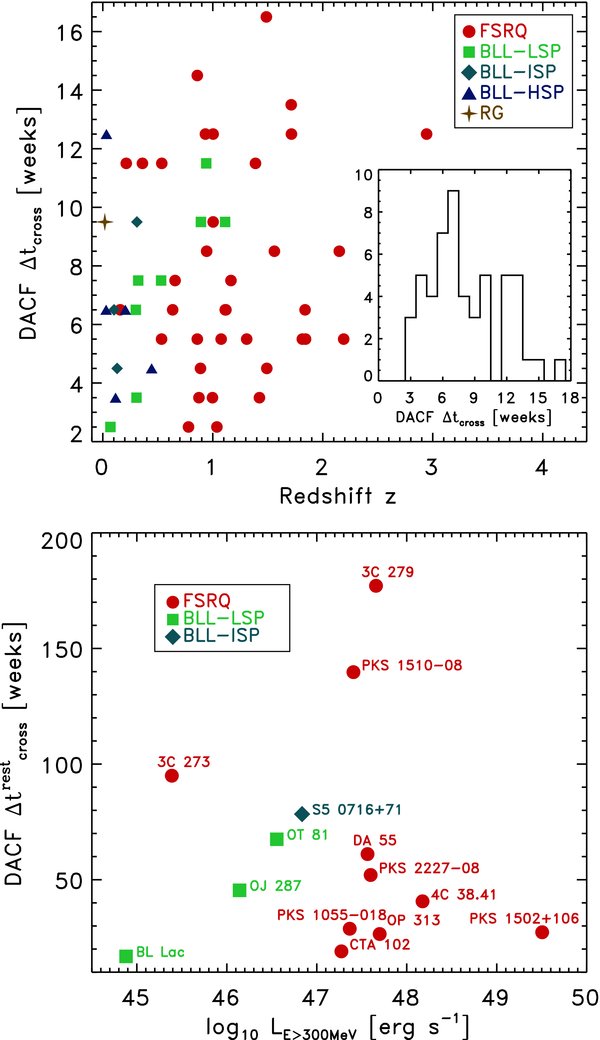
Figure 12. Upper panel: scatter plot of the DACF crossing times Δtcross in weeks vs. the redshift for the 53 brightest and variable LBAS sources with known z (or lower limit). The inset reports the values distribution for the same set. Lower panel: scatter plot of the DACF crossing times in the rest frame of the source (corrected for z and beaming) vs. the total apparent isotropic γ-ray luminosity (E > 300 MeV) in the co-moving frame, defined as in the text, for 15 of the LBAS that are also part of the MOJAVE database. 3C 454.3 is out of the plot range (with Δtcrossrest = 254.3 weeks and log10(LE) = 48.1). All sources in this panel are labeled.
Download figure:
Standard image High-resolution imageThe values of α averaged over the four runs of the SF adopting the four different maximum lags mentioned, are reported for all the 56 sources in Figure 13 against the maximum of the subsequent week-to-week flux variations. In this case, a separation between FSRQs and BL Lacs is not evident, but the difference between the variability behavior of full Brownian gamma-ray sources such as AO 0235+164 and 3C 454.3 and the variability behavior of other powerful gamma-ray blazars such as PKS 1510-08 and PKS 1502+106 is clear. FSRQs such as PKS 1510-08 and PKS 1510+106 are characterized by more de-trended flares (departing from a constant baseline level) or by intermittence, while the most apparently bright FSRQs, like 3C 454.3, have clear long-term trends and stochastic long-term memory (i.e., high-order correlation structure meaning a persistent temporal dependence between observations widely separated in time and low-frequency dominated PDS).

Figure 13. Scatter plot of the PDS power index α evaluated in time domain with the SF (averaged among the SF runs performed with four different maximum time lags, as reported in Figure 11) vs. the observed maximum of the week-to-week flux variations. Most scattered blazars are labeled.
Download figure:
Standard image High-resolution imageIn these weekly light curves no evident sign of periodicity is found, but a more detailed investigation of this aspect will be presented elsewhere using better sampled light curves over only the brightest blazars. In the following two sections, a global analysis (PDS) and a local analysis (functional fit of the flare temporal structure) are applied to more densely sampled light curves (3 day and 4 day bins, integrated flux E > 100 MeV) extracted only for the brightest 28 sources and 10 sources of the LBAS sample, respectively. These light curves starting from a lower energy threshold because of the high brightness and higher statistics are built as described in Section 2.
5. POWER DENSITY SPECTRA OF THE BRIGHTEST BLAZARS
In light curves with binning of a few days, about 15 of the sources are continuously, or almost continuously, detected throughout the 11 month period. For these 15 sources (9 FSRQs and 6 BL Lacs), we used light curves with 3 day binning and for an additional 13 sources (all FSRQs) with slightly lower detection TS, we used light curves with 4 day binning. All light curves were evenly sampled without any data gaps, and a Fourier transform routine was used to compute PDSs.
The power density is normalized to fractional variance per frequency unit (rms2 I−2 day−1), and the PDS points are averaged in logarithmic frequency bins. The white noise level was estimated from the rms of the flux errors and was subtracted for each PDS.
In this section, we present the resulting PDS for a set of individual sources and also the averaged PDS for the two classes, FSRQs and BL Lacs.
There are a number of effects that can, potentially, distort the PDS of our analysis from the "true" long-term variability pattern. This includes stochastic variability within a finite length of observation, systematics in the data, and statistical noise. The last effect dominates at high frequencies so for the determination of PDS slopes we use primarily frequencies up to 0.02 day−1.
The statistical (measurement) errors in the likelihood based light curves were investigated by simulations. These errors were also checked by comparing some light curves with corresponding ones obtained by direct aperture photometry, for which Poisson statistics is valid. This showed that the uncertainty in error estimates is not a significant problem for the brightest sources. For the less bright ones, including all the BL Lacs, this effect does introduce an uncertainty in the estimate of the white noise level in the PDS. The influence of this uncertainty on the PDS slope was estimated by repeating the analysis for a range of possible white noise levels and also by analysis of light curves extracted with different time bins (from 1 to 7 days).
Observational and instrument systematics were investigated by analyzing pulsar light curves extracted from the 11 month data with the same procedure as for the blazars. The most prominent effect is a periodic modulation that is identified with the 55 day precession period of the Fermi spacecraft orbit. This precession is consistent with the addition of the systematic error caused by the variation in effective area due to charged particles during orbital precession. This variation in the LAT effective area is a known effect that is caused by a change in exposure over the orbital precession period (Abdo et al. 2010h). In the PDS for individual blazars this peak is often hidden by the stochastic variability but does show up when averaging the PDS of a number of sources. The frequency bin at this period was not used when PDS slopes were estimated.
The PDS for some of the brighter sources are shown in Figure 14. The source to source differences are most likely dominated by the stochastic nature of the variability process and there is no significant evidence for a break in any of these cases.

Figure 14. Power density spectra computed from 3 day binned light curves for some of the brighter sources. The power density is normalized to rms2 I−2 day−1 and the estimated white noise level has been subtracted.
Download figure:
Standard image High-resolution imageTo reduce the stochastic and statistical fluctuations and study the shape of the PDS for FSRQs and BL Lacs as groups, we averaged the PDS for each of these two classes using all sources detected with TS > 4500. We do this under the assumption that the differences in PDS shape are small compared to the random fluctuations expected due to the action of the (presumed) underlying stochastic process. The resulting averaged PDS for the nine FSRQs is shown in Figure 15. The error bars are asymmetric 1σ errors for the mean over all sources and frequency points averaged in a logarithmic bin. To determine the PDS slope, we focus on the low frequency part, below 0.02 day−1, since at higher frequencies the PDS is more sensitive to systematics due to uncertainties in the white-noise contribution. For frequencies below 0.017, we obtain a best-fit slope of 1.4 ± 0.1.

Figure 15. Top: average power density spectrum (PDS) for the nine brightest FSRQs. White noise level based on light curve error estimates has been subtracted. The error bars are asymmetric 1σ errors of the mean. Our best-fit estimate is a PDS slope of 1.4 ± 0.1. Lower: a comparison of the averaged PDS for three sets of sources, the 9 bright FSRQs from the upper plot (solid line), the 6 brightest BL Lac's (dotted line) and 13 additional FSRQs with TS > 1000 (dashed line). Best-fit slope for the BL Lac and fainter FSRQs is 1.7 ± 0.3 and 1.5 ± 0.2, respectively.
Download figure:
Standard image High-resolution imageThe averaged PDS for the six bright BL Lacs is similarly fitted with a power law up to 0.017 day−1. This gives a slope of 1.7 ± 0.3 with white noise based on the light curve errors. The sample of sources consists of three LSP's (AO 0235+164, PKS 0426 − 380, and PKS 0537 − 441), one ISP (3C 66A), and two HSP's (Mkn 421 and PKS 2155 − 304). Due to the stochastic nature of the variability and the fact that few sources are considered, it is difficult to draw firm conclusions about the differences between the low- and high-peaked BL Lacs. An indication of a trend, however, is that the three LSP's show stronger variability at longer timescales and therefore dominates the determination of the average, steep slope while the two HSP's both have PDS slopes flatter than 1.0. Further observations are needed to see if this trend can be firmly established.
To increase the data sample and to test if source brightness affects the analysis we selected the remaining FSRQs with TS > 1000 and extracted light curves with a 4 day binning. Sources where parts of the light curve had very large flux errors were not used. This resulting sample consisted of 13 sources for which the PDS was averaged and analyzed in the same way as for the brightest sources. For this PDS, we obtain the best-fit slope of 1.5 ± 0.2 in good agreement with the slope for the first sample.
Figure 15 shows all three averaged PDS together for comparison. The difference in the PDS slope for BL Lacs and FSRQs is of marginal significance but we note that the BL Lac slope is consistent with 2 while this is not the case for the FSRQs. None of the averaged PDS shows any significant evidence for the presence of a break although this may still not be excluded for individual sources. From Figure 15 it is also evident that for the present data the fractional variability of the BL Lacs is less than that of the FSRQs, at least up to the 54 day satellite precession peak. The total fractional rms integrated up to 0.017 day−1 in the PDS for the nine FSRQs is 1.35 times that of the six BL Lacs. If the ratio is instead estimated by dividing the PDS for the two groups point by point (which gives equal weight to each frequency point), we get a value of 1.5. Both estimates were made after subtraction of a white noise level corresponding to the flux error values. If the actual white noise level is larger than this, the ratio between the FSRQ and BL Lac fractional variance is most likely larger than our estimate here.
6. TEMPORAL STRUCTURE OF FLARES FOR THE BRIGHTEST BLAZARS
The analysis of individual flares is performed using the extracted 3 day time bin flux (E > 100 MeV) light curves (except for PKS 1502+106 for which we chose 7day time bins), as described in Section 2. For this analysis, we selected the light curves of the 10 sources that exhibited high variability with several flares either separated or partially superimposed (see Table 2.
Table 2. Flare Structure Fit for 3 Day Bin Light Curves of the Brightest Blazars
| 3C 66A | χ2r = 8.0 | Tfl(b) |
|---|---|---|
| flare_time(a) | ξ | |
| 260 | 0.73 ± 0.30 | 14.7 ± 11.9 |
| 280 | −0.19 ± 0.19 | 8.3 ± 1.7 |
| 475 | −0.55 ± 0.33 | 8.8 ± 2.5 |
| 495 | 0.02 ± 0.67 | 11.8 ± 7.9 |
| Average | 0.003 ± 0.207 | 10.88± 3.6 |
| AO 0235+164 | χ2r = 11.4 | Tfl(b) |
| flare_time(a) | ξ | |
| 230 | 0.16 ± 0.07 | 21.7 ±1.5 |
| 251 | 0.61 ± 0.06 | 34.4 ± 1.5 |
| 291 | −0.49 ± 0.11 | 24.0 ± 1.9 |
| 301 | 0.63 ± 0.43 | 21.1 ± 7.9 |
| 380 | 0.04 ± 0.13 | 63.9 ± 8.3 |
| 401 | 0.36 ± 0.09 | 6.3 ± 0.5 |
| 425 | 0.55 ± 0.18 | 47.3 ± 7.2 |
| 460 | −0.04 ±0.38 | 19.1 ± 7.4 |
| 485 | −0.17 ±0.08 | 5.4 ± 0.4 |
| Average | 0.18 ± 0.07 | 27.02 ± 1.74 |
| PKS 0426 − 380 | χ2r = 2.2 | Tfl(b) |
| flare_time(a) | ξ | |
| 395 | 0.10 ± 0.07 | 4.4 ± 0.3 |
| 420 | 0.01 ± 0.30 | 24.2 ± 7.4 |
| 475 | -0.11 ± 0.07 | 25.2 ± 1.8 |
| Average | 0.0003 ± 0.1068 | 17.97 ± 2.52 |
| PKS 0454 − 23 | χ2r = 5.0 | Tfl(b) |
| flare_time(a) | ξ | |
| 236 | −0.39 ± 0.10 | 6.6 ±0.5 |
| 276 | 0.33 ±0.24 | 9.0 ± 2.2 |
| 325 | 0.21 ± 0.08 | 16.0 ± 1.2 |
| 344 | 0.30 ± 0.63 | 13.0 ± 7.9 |
| 375 | 0.25 ± 0.78 | 10.9 ± 8.2 |
| Average | 0.14 ± 0.21 | 11.07 ± 2.34 |
| S4 0917+44 | χ2r = 9.4 | Tfl(b) |
| flare_time(a) | ξ | |
| 364 | 0.0001 ± 0.1650 | 120.1 ± 19.8 |
| 520 | 0.0001 ± 0.0707 | 80.1 ± 5.6 |
| Average | 0.0001 ± 0.0898 | 100.10 ± 10.29 |
| 3C 273 | χ2r = 3.7 | Tfl(b) |
| flare_time(a) | ξ | |
| 229 | 0.13 ± 0.07 | 15.8 ± 1.1 |
| 263 | −0.32 ± 0.03 | 30.2 ± 1.3 |
| 278 | −0.24 ± 0.08 | 6.1 ± 0.4 |
| 290 | −0.22 ± 0.17 | 15.5 ± 2.2 |
| 340 | 0.88 ± 0.04 | 17.0 ± 0.4 |
| 398 | −0.11 ± 0.07 | 4.5 ± 0.3 |
| 445 | −0.76 ± 0.04 | 68.0 ± 1.5 |
| 483 | −0.31 ± 0.09 | 30.7 ± 2.3 |
| 525 | −0.46 ± 0.11 | 45.7 ± 3.6 |
| Average | −0.16 ± 0.03 | 25.93 ± 0.89 |
| 3C 279 | χ2r = 3.7 | Tfl(b) |
| flare_time(a) | ξ | |
| 238 | −0.33 ± 0.24 | 11.0 ± 2.3 |
| 332 | −0.22 ± 0.08 | 17.0 ± 1.2 |
| 355 | −0.41 ± 0.03 | 28.4 ±1.3 |
| 398 | −0.67 ± 0.05 | 71.9 ± 4.2 |
| 419 | 0.29 ± 0.08 | 22.4 ± 1.6 |
| Average | −0.27± 0.05 | 30.11 ± 1.07 |
| PKS 1502+106 | χ2r = 4.4 | Tfl(b) |
| flare_time(a) | ξ | |
| 242 | −0.20 ± 0.10 | 40.7 ± 3.8 |
| 305 | −0.71 ± 0.12 | 41.6 ± 2.9 |
| 336 | 0.11 ± 0.11 | 31.6 ± 3.2 |
| 365 | 0.13 ± 0.14 | 21.3 ± 3.4 |
| 405 | 0.28 ± 0.09 | 55.6 ± 4.1 |
| 485 | −0.18 ± 0.08 | 57.2 ± 4.1 |
| 525 | −0.05 ± 0.07 | 36.8 ± 2.6 |
| Average | −0.09 ± 0.04 | 40.67 ± 1.31 |
| PKS 1510 − 08 | χ2r = 17.8 | Tfl(b) |
| flare_time(a) | ξ | |
| 260 | −0.52 ± 0.12 | 25.1 ± 2.0 |
| 381 | −0.39 ± 0.10 | 19.7 ± 1.5 |
| 445 | 0.07 ± 0.01 | 24.2 ± 0.3 |
| 480 | 0.25 ± 0.08 | 11.1 ± 0.8 |
| Average | −0.15± 0.04 | 20.00 ± 0.66 |
| 3C 454.3 | χ2r = 7.3 | Tfl(b) |
| flare_time(a) | ξ | |
| 235 | 0.24 ± 0.16 | 20.3 ± 3.8 |
| 255 | 0.29 ± 0.08 | 18.0 ± 1.3 |
| 272 | 0.24 ± 0.36 | 22.2 ± 7.9 |
| 295 | 0.44 ± 0.28 | 32.2 ± 8.2 |
| 327 | 0.25 ± 0.13 | 41.8 ± 4.4 |
| 378 | -0.42 ± 0.10 | 28.5 ± 2.2 |
| 490 | 0.48 ± 0.11 | 59.4 ± 4.7 |
| Average | 0.22 ± 0.07 | 31.79 ± 1.98 |
Notes. aDay of the flare peak (DoY 2008 unit). bFraction of days.
We use the following function to reproduce the time profile of a single flare:
where Fc represents an assumed constant level underlying the flare, F0 measures the amplitude of the flares, t0 describes approximatively the time of the peak (it corresponds to the actual maximum only for symmetric flares), and Tr and Td measure the rise and decay time. This function is well suited to study both the duration and symmetry of the individual flares. Double exponential forms for the functional fit were used in the past to fit individual blazar flare pulses (Valtaoja et al. 1999). Other and more general functions are used in gamma-ray burst science (see, for example, Norris et al. 2000, 2005; Vetere et al. 2006). The time of the maximum of a flare can be easily computed from the first derivative of Equation (7):
which is equal to t0 for Td = Tr. A good estimate of the total duration of the flare is

which, for symmetric flares, corresponds to the interval where the flux level is reduced to about 20% of the peak value.
As a first step, we identify the flare to be fitted and detect the time of the peak, which was kept frozen in the fitting procedure unless the flare was clearly superimposed on to a slow trend. We build a function with as many components as the flares' number and perform a fit for each source with the function of Equation (7). To verify the validity of this procedure, we analyzed the distribution of the residuals, calculated by subtracting the observed flux from the modeled one and dividing by the flux errors, which should be compatible with a constant level. Figure 16 shows the light curves of six sources with the fit function superimposed, 3C 66A, PKS 0426 − 380, PKS 0454 − 234, 3C 273, 3C 279, and 3C 454.3. This procedure was satisfactory for the majority of the flares, but for a few events it did not provide quite good fits. For instance, in the case of the first flare 3C 273 some data points lie above the fitting curve and this discrepancy could be due to events of short duration which were not well sampled.

Figure 16. Six representative light curves (E > 100 MeV) of bright blazars (3C 66A, PKS 0426 − 380, PKS 0454 − 234, 3C 273, 3C 279, and 3C 454.3) obtained with 3 day bins. Data points represent detected flux values having a TS greater than 9, and the continuous (blue) curve represents the best-fit function described in Equation (7).
Download figure:
Standard image High-resolution imageWe also defined the following parameter to describe the symmetry of the flares:
which spans between −1 and 1 for completely right and left asymmetric flares, respectively.
The value of ξ can provide a useful indication of the physical evolution of the flare. Those having a marked asymmetric profile can be explored in terms of a fast injection of accelerated particles and a slower radiative cooling and/or escape from the active region. Symmetric flares, with or without a long standing plateau, can be related to the crossing time of radiation (or particles) through the emission region or can be the result of the superposition of several episodes of short duration. The ξ parameter is used to define three different classes of flares: (1) symmetric flares where −0.3 < ξ < 0.3, (2) moderately asymmetric flares when −0.7 < ξ < −0.3 or 0.3 < ξ < 0.7, and (3) markedly asymmetric flares when −1.0 < ξ < −0.7 or 0.7 < ξ < 1.0. The parameters are listed in Table 2, and their distributions are shown in Figure 17.

Figure 17. Distributions of the flare pulse parameters for the cumulated 10 bright blazars analyzed with this technique. Values of ξ above and Tfl below are shown.
Download figure:
Standard image High-resolution image
We also calculated the weighted mean of these parameters to study the general properties of the time profiles of gamma-ray flares. We obtain 〈ξ〉 = −0.084 ± 0.009 and 〈Tfl〉 = 11.87 ± 0.12. Looking at the results of the fitting procedure and the weighted means we can see that the list of brighter sources shows two different types of temporal profiles: the sources with a stable baseline with a sporadic flaring activity and the sources with a strong activity with complex and structured features. Based on our analysis we can put 3C 66A, PKS 0426 − 380, S4 0917+44, and PKS 0454 − 234 in the first class of objects and 3C 279, 3C 273, 3C 454.3, PKS 1502+106, AO 0235+164, and PKS 1510 − 08 in the second one, while no evidence of very asymmetric profiles is found. In Figure 16, we report cases of both classes to show the different time profiles. Note that for the majority of events the uncertainties on ξ are small; however, for a few flares of 3C 66A, AO 0235+164, and PKS 0454 − 23, the resulting asymmetries are not safely estimated. In fact, despite their large values the occurrence of symmetricity in moderately asymmetric profiles cannot be excluded within 1 standard deviation.
We found only four markedly asymmetric flares: for 3C 66A (DoY 2008 260 ξ = 0.73 ± 0.30), 3C 273 (DoY 2008 340 and 445, ξ = 0.88 ± 0.04 and ξ = −0.76 ± 0.04, respectively), and PKS 1502+106 (DoY 2008 305, ξ = −0.71 ± 0.12), where two of them have rise times longer than the decays. In the case of 3C 66A, the flare was rather short and the resulting uncertainty on ξ is large; therefore no firm conclusion on its shape can be established. The two flares of 3C 273 clearly exhibit different profiles. Note that the highest point of flare at epoch 340 is well above the fitting curve implying the possibility of an even higher value of ξ, whereas the subsequent and much longer flare (DoY 2008 445), which has a very well established negative asymmetry, may be due to confusion because of the partial superposition of low amplitude and short events, not individually detectable. 3C 273 also exhibited a couple of exceptional flares in 2009 September (Abdo et al. 2010f) in which it reached a very high level, and the light curves were very finely sampled. In both episodes rise times were shorter than the subsequent decays. Similarly, PKS 1502+106 exhibited a markedly asymmetric outburst in 2008 August, resolved with a daily binning (Abdo et al. 2010d).
7. SUMMARY AND CONCLUSIONS
Gamma-ray light curves (Figures 1 and 2) and variability properties of the 106 LBAS blazars (0FGL list; Abdo et al. 2009a, 2009b) collected during the first 11 months of the all-sky survey by Fermi LAT are presented. This represents a first systematic study of gamma-ray variability over a consistent set of homogeneously observed blazars.
The light curves of 84 of these sources have at least 60% of the 47 weekly bins with flux detection of TS>4 (≳2σ), and 56 have also a significant excess variance (Table 1). The low gamma-ray brightness states interposed among the flares are studied, for the first time as well, and high flux states do not exceed 1/4 of the total light curve range (most sources being active in periods shorter than 5% of the total light curve duration). FSRQs and LSP/ISP BL Lac objects showed the largest variations, as expected, with the high energy SED component peaked at MeV and GeV bands. HSP BL Lac object shows lower variability (with remarkable exception of ON 325), and their emission is persistent, easily detected in all the weeks of the considered period, and also because of their smaller redshift (Section 3).
In these first 11 months of Fermi mission, PKS 1510 − 08, PKS 1502+106, 3C 454.3, 3C 279, and PKS 0454 − 234 (all FSRQs) are observed to be the brightest and most violently variable gamma-ray blazars. In a few cases this was also true for BL Lac objects (3C 66A and AO 0235+164 for example). In particular, PKS 1502+106 (OR 103), 4C 38.41 (S4 1633+38), and 3C 454.3 were also the most intrinsically gamma-ray powerful blazars in these months. The other sources appear distributed with decreasing observed subsequent maximum variations with increasing redshift. Different autocorrelation patterns, central lag peak amplitudes, zero crossing times, different temporal trends, and power-law indices are shown by the DACF and SF, pointing out different timescales and variability modes (more flicker-dominated or Brownian-dominated). The weekly PDSs evaluated using the SF in blind mode point out a 1/fα trend with α values mostly distributed between 1.1 and 1.6. Light curves of AO 0235+164 and 3C 454.3 are observed to be fully Brownian (i.e., with the steepest PDS slopes, α ⩾ 2) with longer emission cycles and sustained flares that could identify more massive central black holes. Other powerful sources such as PKS 1510 − 08 and PKS 1510+106 show variability behavior half-way between the two classes above (with α ∼ 1.3), showing intermittence and de-trended complex superposed flares, respectively. The DACF crossing lag times are found mostly distributed between 4 and 13 weeks with a peak at 7 weeks.
The mean variability properties for the brighter sources are studied in more detail by calculating an average PDS for each of the two main blazar types, FSRQs (nine sources) and BL Lacs (six sources). For both types, the average PDS is described by a power law without any evidence of a break in the frequency range where our sensitivity is best (0.003 to at least 0.017 day−1). The power-law index for the averaged PDS was estimated to be 1.4 ± 0.1 and 1.7 ± 0.3 for the FSRQs and BL Lacs, respectively. The BL Lac sources show a large spread in PDS slopes with an indication of trend such that the PDS is steeper for LSPs than for the HSPs. Further observations are needed to establish this trend, but we note that in the present data the two brighter HSP's (Mkn 421 and PKS 2155 − 304) have PDS slopes of order 1 or flatter. For Mkn 421, we can compare this with the corresponding result for soft X-rays. Analyzing the RXTE ASM X-ray light curve for this source, we obtain a well-defined power-law index of 1.04 ± 0.05. Aside from Mkn 421, the best available long-term X-ray light curve is that of the FSRQ 3C 279. For this source, Chatterjee et al. (2008) found a slope of 2.3 ± 0.3 for the X-ray band and 1.7 ± 0.3 for the optical. In this case our result in the gamma-ray band, both the average for FSRQs and for 3C 279 itself (1.6 ± 0.2), is closer to the PDS slope in the optical than in X-rays. More generally, the gamma-ray PDSs of the bright Fermi LAT sources have slopes similar to those obtained from long-term optical and radio light curves (Section 4). For the X-ray band, the situation is less clear since only a few sources have good enough long-term light curve to allow for a comparison.
The power density excess (above the noise level) in the 0.003–0.017 day−1 range was found to correspond to a mean rms fractional variability (rms/I2) of 0.50 for the nine bright FSRQs and 0.37 for the six brightest BL Lacs. These results imply that in the LAT energy range and presently accessible timescales the FSRQs exhibit a larger relative variability than the BL Lac's.
Gamma-ray variability observed in these LBAS blazars can be described both as essentially steady sources with perturbations or as a series of discrete, though possibly overlapping, flares produced, for example, by traveling shock fronts. The emission could be produced in multiple regions forming an inherently inhomogeneous blazar zone or in an essentially homogenous region where all particles are accelerated, depending on the particular source considered.
Random walk processes producing such PDS variability slopes, such as instabilities and turbulence in the accretion flow through the disk or in the jet, can cause the intermittent behavior observed in several of these Fermi LAT light curves. These are stochastic processes, mostly characterized by the presence of a large number of weakly correlated elements which appear at random, live only a short time, and decay. Steep PDS slopes mean more Brownian-dominated regimes characterized more by long memory and self-similarity. Large flares likely arise from the sudden acceleration of relativistic electrons, related to bulk injections of new particles and/or strong internal shocks (Mastichiadis & Kirk 1997; Spada et al. 2001; Böttcher & Dermer 2010). These type of PDSs could be related to mass accretion avalanches providing shot pulses: larger (and longer) shots contribute to the low-frequency part of the PDS, while smaller and shorter shots determine the power law decline at high frequencies. In this case, variability would be explained as disturbances or inhomogeneities in the accretion process, opposite to intermittence, which can be evidence of dissipation in the jet and described by turbulence-driven processes. Furthermore, well identified GeV recurrent characteristic timescales, pointed out by breaks in the PDS, can be related linearly to the mass of the central supermassive black hole (Markowitz 2006; Dermer 2007; Wold et al. 2007; McHardy 2008), as happens for X-ray variability timescales in Seyfert galaxies, but more detailed analysis with improved sampling is needed to shed light on this issue.
Finally, the local analysis of flare temporal shapes for the brightest sources revealed and confirmed in a quantitative way different temporal profiles: stable baseline with sporadic flaring activity or strong activity with complex and structured temporal features. The average durations of the fitted flares varied from about 10 days up to 100 days in the case of S4 0917+44. In other very bright flares, timescales as short as a fraction of a day have been observed (3C 273, PKS 1510 − 089) and in some cases the light curves were structured in a series of shorter peaks. The low mean asymmetry of the events analyzed in Section 6 can be then explained by the superposition of a series of peaks, even if the light curves analyzed are already resolved with a short, 3 day sampling. A marked asymmetric profile can be explained in terms of a fast injection of accelerated particles and a slower radiative cooling and/or escape from the active region and could be considered cooling-dominated flares. The fast rise and slower decay can be evidence for a dominant contribution by Comptonization of photons produced outside the jet (Sikora et al. 2001). Gamma-ray flares produced by short-lasting energetic electron injections and at larger jet opening angles are predicted to be more asymmetric showing much faster increase than decay, the latter determined by the light travel time effects. On the other hand, symmetric flares, with or without a long standing plateau, can be related to the crossing time of radiation (or particles) through the emission region, dominated by geometry and spatial scales (Takahashi et al. 2000; Tanihata et al. 2001). Flares observed at or above the peak energy reflect the scale of the source along the line of sight and are symmetric in the cylindrical geometry of the active regions (Eldar & Levinson 2000; Sokolov et al. 2004). The result of the superposition and blending of several episodes of short duration could also provide symmetric flare shapes (Valtaoja et al. 1999).
The presentation of gamma-ray light curves of a consistent set of blazars observed in homogeneous conditions by Fermi LAT over almost one year, and our systematic variability characterization showed properties in some ways similar to the radio-band and optical variability. Variation amplitudes, flare durations, PDS slope values, preliminary hints for typical timescales, and morphology of the flares can be used to support the identification of the correct source class for newly discovered unidentified sources. Basically, an LAT gamma-ray blazar is displaying two "flavors" of variability: a rather constant baseline with sporadic flaring activity showing also intermittence and characterized by flatter PDS slopes resembling the red noise, flickering, fluctuations, and a few sources showing strong activity with complex and structured time profiles characterized by the long memory and steeper PDS slopes of random walk processes. Finally, our results can also serve as a preparatory study for more detailed analysis and modeling that are possible with the brightest and most variable sources through better sampling and time resolution.
The Fermi LAT Collaboration acknowledges generous ongoing support from a number of agencies and institutes that have supported both the development and the operation of the LAT as well as scientific data analysis. These include the National Aeronautics and Space Administration and the Department of Energy in the United States, the Commissariat à l'Energie Atomique and the Centre National de la Recherche Scientifique/Institut National de Physique Nucléaire et de Physique des Particules in France, the Agenzia Spaziale Italiana and the Istituto Nazionale di Fisica Nucleare in Italy, the Ministry of Education, Culture, Sports, Science, and Technology (MEXT), High Energy Accelerator Research Organization (KEK) and Japan Aerospace Exploration Agency (JAXA) in Japan, and the K. A. Wallenberg Foundation, the Swedish Research Council, and the Swedish National Space Board in Sweden.
Additional support for science analysis during the operations phase is gratefully acknowledged from the Istituto Nazionale di Astrofisica in Italy and the Centre National d'Etudes Spatiales in France.
S.C. acknowledges funding by grant ASI-INAF n.I/047/8/0 related to Fermi on orbit activities.
The Fermi LAT Collaboration extend thanks to the anonymous referee who made useful and constructive comments.
Facilities: Fermi (LAT) - .
APPENDIX
Data appearing in the plots of Figures 1 and 2 are available in Table 3.
Table 3. Tabulated Data of the Weekly Flux Light Curves Reported in Figures 1 and 2
| 0FGL name | Weekly | Flux (E > 300 MeV) | Error | TS | Upper |
|---|---|---|---|---|---|
| Indexa | [10−6 photons cm−2 s−1] | Limit | |||
| J0017.4-0503 | 0 | 0.0565 | 0.0107 | 64.2 | 0.0000 |
| J0017.4-0503 | 1 | 0.0141 | 0.0067 | 7.5 | 0.0291 |
| J0017.4-0503 | 2 | 0.0158 | 0.0072 | 10.3 | 0.0293 |
| J0017.4-0503 | 3 | 0.0514 | 0.0109 | 49.5 | 0.0000 |
| J0017.4-0503 | 4 | 0.0276 | 0.0107 | 11.1 | 0.0470 |
| J0017.4-0503 | 5 | 0.0265 | 0.0090 | 15.8 | 0.0428 |
| J0017.4-0503 | 6 | 0.0330 | 0.0099 | 20.3 | 0.0506 |
| J0017.4-0503 | 7 | 0.0276 | 0.0084 | 24.6 | 0.0426 |
| J0017.4-0503 | 8 | 0.0089 | 0.0052 | 6.6 | 0.0189 |
| J0017.4-0503 | 9 | 0.0278 | 0.0088 | 18.2 | 0.0437 |
Notes. aThe relation between weekly index and time is as follows. The week with index 0 begins on Aug. 5, 2008 at 00:00:00 UTC, MJD 54683, MET 239587200, so the week with index i begins on MJD 54683+7xi and ends on MJD 54690+7xi.
Only a portion of this table is shown here to demonstrate its form and content. A machine-readable version of the full table is available.
Download table as: DataTypeset image