


ABSTRACT
Perpendicular diffusion coefficients and mean free paths of cosmic particles are computed for an anisotropic Alfvénic turbulence spectrum corresponding to the Goldreich–Sridhar model by employing an enhanced nonlinear guiding center theory. The calculations are important for understanding cosmic ray propagation in the Galaxy and in the solar system. In addition, the knowledge of diffusion coefficients is also useful for modeling charged particles which experience diffusive shock acceleration in supernova remnants and at interplanetary shock waves. To replace the parallel diffusion coefficient in our equation for the perpendicular diffusion coefficient, we employ different models such as quasilinear results and phenomenological models. The results are compared with those derived earlier. We demonstrate that the choice of the turbulence model as well as the choice of the model for the parallel diffusion coefficient has a strong influence on the perpendicular diffusion coefficient.
Export citation and abstract BibTeX RIS
1. INTRODUCTION
The scattering of energetic charged particles (e.g., cosmic rays) occurs due to the interaction between the particles and the turbulent magnetic fields of the interplanetary or interstellar plasma  . To understand this scattering mechanism is important for modeling the propagation of cosmic particles in the Galaxy (see, e.g., Büsching & Potgieter 2008; Büsching et al. 2008) and for describing particles which experience diffusive shock acceleration (see, e.g., Kirk et al. 1988; Berezhko & Völk 2007). The latter mechanism is believed to be responsible for the origin of cosmic rays. In the physics of the solar system/solar wind, the knowledge of this scattering process is important for the study of solar modulation of galactic cosmic rays (see, e.g., Alania et al. 2010; Engelbrecht & Burger 2010; Hitge & Burger 2010; Wawrzynczak & Alania 2010) and for understanding solar energetic particles (see, e.g., Dröge & Kartavykh 2009; Dröge et al. 2010). Charged particle transport is also important in the physics of laboratory plasmas and fusion devices (see, e.g., Spatschek 2008; Hauff & Jenko 2008). While cosmic ray diffusion is generally believed to be a well-developed subject (see reviews in Schlickeiser 2002 and in Shalchi 2009b), in reality many outstanding issues exist. These are related both to the theory of turbulence with which the cosmic rays interact and to the quantitative description of the propagation.
Since large-scale magnetic fields such as the Galactic magnetic field break the symmetry of the physical system, one has to distinguish between transport of particles along and across the mean magnetic field. Spatial diffusion has to be described by a whole diffusion tensor κij. In the present paper, we use a Cartesian system of coordinates in which the z-axis points in the direction of the mean magnetic field, i.e.,  . The components κij with i, j = x, y are the perpendicular diffusion coefficients and κ∥ ≡ κzz is the parallel diffusion coefficient. To achieve a complete description of cosmic ray propagation and acceleration, one has to know all components of the diffusion tensor. The assumption of isotropic scattering, i.e., κxx = κyy = κzz and κxy = κyx = 0, is, in general, invalid even if the turbulence is isotropic (see Shalchi & Dosch 2009).
An important ingredient in the theory of particle scattering is the model of magnetic fluctuations. For describing particle transport in the solar system a phenomenological slab/2D composite model (see, e.g., Bieber et al. 1994; Shalchi et al. 2006) is frequently used. In the latter model, which is also known as the two-component model, it is assumed that interplanetary fluctuations can be described as a superposition of fluctuations with wave vectors parallel to the ambient large-scale magnetic field (so-called slab modes) and perpendicular to the mean field (so-called two-dimensional (2D) modes). This model results in a maltese cross structure of magnetic correlations. This model was developed to account for the solar wind observations which it does well by adjusting the intensity of two components (see, e.g., Matthaeus et al. 1990; Weinhorst & Shalchi 2010). From the theoretical point of view, as well as from the point of numerical testing, this standard model is rather vulnerable. Indeed, two-dimensional fluctuations are consistent with the theory of weak Alfvénic turbulence (see Ng & Bhattacharjee 1996; Lazarian & Vishniac 1999; Galtier et al. 2000), but the prediction of this analytical theory is the strengthening of the cascade with the decrease of the turbulence scale. Therefore, 2D fluctuations can describe Alfvénic turbulence only over a limited range of scales. In addition, slab modes do not arise naturally in magnetohydrodynamic (MHD) numerical simulations with large-scale driving (see Cho & Lazarian 2002, 2003). Nevertheless, the factors above cannot be used to dismiss the slab/2D model at present. First of all, the solar wind exhibits a relatively short inertial range. Moreover, the driving of turbulence there is far from being isotropic as in simulations. Further research will clarify these points.
In the interstellar medium (ISM), the inertial range of fluctuations is much more appreciable from hundreds of kilometers to dozens of parsecs (see Armstrong et al. 1995; Chepurnov & Lazarian 2010). In this situation, the details of the driving of turbulence should not be so important and therefore the correspondence with theoretical expectations and numerical simulations of turbulence with the uniform large-scale driving should be applicable.4
For Alfvénic turbulence with uniform large-scale driving an appealing model of turbulence was proposed by Goldreich & Sridhar (1995, henceforth GS95). The key element of the model is the so-called critical balance which is the rough equality between the timescale of the eddies' turnovers perpendicular to the local magnetic field and the periods of waves associated with the eddies. This equality is frequently expressed following the GS95 convention in terms of parallel and perpendicular wavenumbers k||vA ∼ k⊥vk, where vk is the turbulent velocity at scale k, vA is the Alfvén velocity, and k|| and k⊥ are parallel and perpendicular wave numbers. The caveat here is that the wavenumbers are defined in the global magnetic field frame of reference, and this may be misleading. The critical balance is the condition satisfied only in the frame related to the local magnetic field.5 In what follows we use the parallel and perpendicular wavenumbers but understand them in terms of wavelets, which allow the choice of the local magnetic field (see Kowal & Lazarian 2010).
In the GS95 model, the cascading is Kolmogorov type in terms of motions perpendicular to magnetic field lines. Indeed, the motions of the fluid perpendicular to the magnetic field are not constrained by magnetic tension and therefore the energy cascading rate is ∼v2l/tcas ∼ v2l/(l/vl), which induces the Kolmogorov scaling, namely, E(k⊥) ∼ k5/3⊥. Here, we used the turbulent velocity vl at scale l and the cascading time tcas at scale l. Combining the critical balance with the Kolmogorov cascading one gets the relation between the characteristics of the MHD eddies, i.e., the relation between k⊥ and k||, namely k|| ∼ k2/3⊥, which reflects the fact that Alfvénic motions get more and more anisotropic at small scales.
The GS95 theory was formulated under the assumption that the injection happens with Alfvénic velocity at the injection scale, which is a rather special case. However, the model can be generalized for both super-Alfvénic and sub-Alfvénic injection velocities. For the super-Alfvénic case the generalization is straightforward. One expects the turbulence to evolve along the Kolmogorov cascade while the turbulent velocity is much larger than the Alfvén velocity, with magnetic fields being advected by hydrodynamic motions. At the scale at which the turbulent velocity becomes equal to the Alfvén velocity the GS95 cascade starts. The case of sub-Alfvénic driving is a little trickier as the cascade initially develops as weak Alfvénic turbulence. In this cascade k|| stays constant and k⊥ increases, which eventually ensures that the critical balance is satisfied. At this scale, the turbulence is already strongly anisotropic and the relations for the k⊥ and k|| are modified (Lazarian & Vishniac 1999).
While the subject of MHD turbulence, in particular, its exact scaling, intermittency, dynamical alignment, and locality of the cascade are hotly debated in the literature (see Boldyrev 2005, 2006; Beresnyak & Lazarian 2006, 2009b, 2010; Gogoberidze 2007; Matthaeus et al. 2008), the keystone of the GS95 model, namely the critical balance, remains. Therefore, for the rest of the paper we shall assume the validity of GS95 scalings but adopt the analytical description of Alfvénic turbulence of Lazarian & Vishniac (1999), which covers not only the case of injection velocity vinj equal to the Alfvén velocity vA, but also vinj < vA.
The GS95 picture differs substantially both from the slab/2D composite model and the turbulence model of Iroshnikov (1964) and Kraichnan (1965). The latter model of isotropic Alfvénic turbulence strongly contradicts the numerical simulations. The former, i.e., the slab/2D composite, is also anisotropic, but in the GS95 model there are no slab waves and the fluctuations, although anisotropic, change both parallel and perpendicular dimensions coherently. In contrast, in the 2D model the parallel scale stays the same while the perpendicular scale changes, which is a feature of weak Alfvénic turbulence. The main features of the GS95 model were successfully tested numerically using different numerical schemes and approaches (Cho & Vishniac 2000; Maron & Goldreich 2001; Cho et al. 2002; Müller & Biskamp 2000; Beresnyak & Lazarian 2009b). The GS95 model of Alfvénic turbulence was proven to hold in the presence of compressibility (Cho & Lazarian 2002, 2003; Beresnyak & Lazarian 2006; Kowal & Lazarian 2010). Thus, we feel that it is safe to adopt this model for the rest of the paper. We believe that the possible inevitable ramifications of the model will not dramatically alter our results. It is general knowledge that the Kolmogorov model of incompressible hydro turbulence is incomplete, but this does not prevent its wide practical use.
A key feature of the GS95 model of Alfvénic turbulence is its high anisotropy. Due to this anisotropy, the calculations of Chandran (2000), who used the Alfvénic energy tensor motivated by the GS95 model to compute the cosmic ray diffusion coefficient along the mean magnetic field, provided a substantial reduction of the scattering rates. The energy tensor of Chandran (2000) was rather ad hoc, however. To provide better accuracy Yan & Lazarian (2002, 2004) used a tensor based on the numerical study of Cho et al. (2002, henceforth CLV02). The authors obtained the scattering rates which were appreciably larger than those of Chandran (2000). In the present paper, we complement this previous work by combining the latter correlation tensor with the latest theory for perpendicular diffusion, to compute the cosmic ray diffusion coefficient across the mean magnetic field. For comparison we also show results obtained for a slab/2D model which was used earlier to approximate solar wind turbulence.
The organization of the present paper is as follows. In Section 2, we discuss and compare two models which have been developed to approximate turbulence. In Section 3, we present an integral equation for the perpendicular diffusion coefficient and we combine this equation with the different turbulence models. As shown there, the parallel mean free path has to be known in order to compute diffusion coefficients across the mean magnetic field. Therefore, we discuss different models for the parallel diffusion coefficient in Section 4. In Section 5 we show the results for the diffusion coefficient across the mean magnetic field, and in Section 6 we present a summary and conclusion.
2. THE CORRELATION TENSOR OF MAGNETIC TURBULENCE
An important ingredient in theories of cosmic ray diffusion is the magnetic correlation tensor. In this section, we discuss some properties of this quantity. Thereafter, we review two models that were developed earlier in order to approximate interplanetary and interstellar turbulence.
2.1. Definition of Wave Vectors
Wave vectors are usually defined in the system of mean or global magnetic field. This can be a confusing point when one deals with the modern understanding of the GS95 model of turbulence. There the wave vectors should be understood more in the sense of wavelets rather than normal Fourier transforms, as the parallel and perpendicular wavenumbers are given with respect to the local direction of the magnetic field. Incidentally, such local perturbations are actually sampled by cosmic rays streaming along the actual turbulent magnetic field.
Various approaches for defining the parallel and perpendicular scales have been employed (see a comprehensive discussion of various techniques in Beresnyak & Lazarian 2009b). The essence of those techniques is defining the local direction of the magnetic field and calculating the correlations with respect to this direction. This does not involve the separation of scales assumption, as the local magnetic field can be defined at any scale. It is important that different techniques provide the same answer for the relation of the parallel and perpendicular scales of eddies (see Beresnyak & Lazarian 2009b and references therein), which, as we mentioned earlier, for the sake of historical continuity we identify with the inverse of wavenumbers k|| and k⊥.
At the same time, in the earlier theories (and even in the original GS95 publication) this distinction was not considered. Therefore, this issue is of potential confusion. In what follows, we consider k|| and k⊥ in the local system of reference whenever the GS95 model is mentioned.
2.2. The Magnetic Correlation Tensor
The time-dependent correlation tensor of magnetic fluctuations is defined as

A common assumption is that all tensor components of the magnetic fluctuations have the same temporal behavior, corresponding to  . The function
  is usually called the dynamical correlation function. For this function, different models have been discussed previously. Exponential decay of perturbations is something that has been suggested by many authors and which is roughly consistent with turbulence studies. Bieber et al. (1994), for instance, have proposed the so-called damping model of dynamical turbulence in which the dynamical correlation function is given by
with the wave vector dependent correlation time  . This form was also used by Shalchi et al. (2006), where the so-called nonlinear anisotropic dynamical turbulence (NADT) model has been discussed. In the GS95 model the time τ is different, thus, for instance, in Chandran (2000) the time
is used, with the Alfvén speed vA and the characteristic length l. Such dynamical correlation effects could be important in describing the propagation of charged particles along the mean magnetic field. In particular, for reproducing parallel mean free paths of low energetic electrons in the solar system, dynamical turbulence effects are essential (see, e.g., Bieber et al. 1994; Shalchi et al. 2006). The situation is different if one investigates diffusion of particles across the mean magnetic field. As shown by Shalchi et al. (2006), perpendicular diffusion coefficients are only weakly influenced by the turbulence dynamics. Since we focus on particles which propagate much faster than the Alfvén speed (v ≫ vA) we apply the magnetostatic approximation by setting  and, therefore,
  . In the following, we discuss the static tensor
  .
.
According to Matthaeus & Smith (1981), the correlation tensor for arbitrary but axisymmetric turbulence is given by
Here we have neglected magnetic helicity. The function A(k∥, k⊥) describes the turbulence spectrum. In the following paragraphs, we discuss two analytical forms that have been proposed previously. Those forms have to satisfy the normalization condition
Here we have used the wave vector components along and across the mean magnetic field k∥ and k⊥, respectively. Equation (4) takes into account the solenoidal constraint . Furthermore, we have assumed axisymmetric turbulence and a symmetric spectrum with A(k∥, k⊥) = A(−k∥, k⊥).
2.3. The Tensor of CLV02
The GS95 model does not predict the exact form of the tensor of Alfvénic perturbations. It only states that most energy will be in the state of critical balance. In what follows we shall adopt the tensor of magnetic field empirically obtained in CLV02. These authors argued that the actual tensor contains so-called Castang functions, but in a simplified form can be written as
The factors in this model were chosen to satisfy the normalization constraint (Equation (5)). Furthermore, we have used the ratio of the turbulence and the mean field EB ≡ δB/B0 and the characteristic length scale l. The form of tensor given by Equation (6) was adopted for calculations in Yan & Lazarian (2002, 2004, 2008). In contrast, Chandran (2000) adopted a steep cutoff of the modes beyond the critical balance k|| ∼ k2/3⊥ and thus underestimated the efficiency of the cosmic ray scattering.
2.4. The Slab/2D Turbulence Model
A lot of work has been done to improve our understanding of turbulence and charged particle transport in the solar system. Here, one needs to take into account the limited inertial range of turbulent motions over which the turbulence is present. While usually in talking about turbulence one disregards the peculiarities induced by the injection scale and the dissipation scale and concentrates on the inertial range, it is not clear whether this is possible to do for the solar wind.
While numerical simulations provide evidence in favor of the Goldreich–Sridhar spectrum, other models may be applicable to describe the transient state of the solar wind fluctuations. In particular, an empirical model of slab and 2D fluctuations was proposed (see Matthaeus et al. 1990) and was widely used for describing the properties of turbulence. In this model, the 2D fluctuations may be associated with the theoretically motivated fluctuations of the weak Alfvénic turbulence (see Lazarian & Vishniac 1999; Galtier et al. 2000), while the origin of the slab Alfvén modes may be due to the particular driving of turbulence.6
Matthaeus et al. (1990) have shown that magnetic correlations in the solar wind have the form of a maltese cross. These observations support the assumption that there are slab modes (defined as  ) superposed with dominant 2D modes (defined as
  ). The latter model is also known as the slab/2D composite model. In this case, the spectrum A(k∥, k⊥) is defined as
with the one-dimensional (1D) spectra of the slab modes gslab(k∥) and the 2D modes g2D(k⊥), respectively. Later, Weinhorst & Shalchi (2010) used an enhanced slab/2D model to reproduce the observations presented by Matthaeus et al. (1990). Although observations in the solar wind support the analytical form (Equation (7)), there has also been some theoretical work showing that the slab/2D model is indeed a good approximation for interplanetary turbulence. The theory of nearly incompressible MHD, for instance, predicts a collapse in dimensionality making turbulence in the solar wind a superposition of dominant 2D modes and a slab component (see Zank & Matthaeus 1993). The theory of plasma instabilities also predicts the existence of 2D modes (see Stockem et al. 2006).
Recently, Hunana & Zank (2010) have formulated a nearly incompressible theory of MHD in the presence of a static large-scale inhomogeneous background. This theory was primarily developed to describe solar wind turbulence where the assumption of slab/2D turbulence with the dominance of the 2D component has often been used. Those authors have shown that, compared to the homogeneous description of Zank & Matthaeus (1993), the reduction of dimensionality from three-dimensional (3D) to 2D turbulence is only weak. Close to the Sun, however, where the large-scale magnetic field can be considered as purely radial, the collapse of dimensionality to 2D is complete. It seems that in the solar system the heliocentric distance controls the structure of turbulence.
For a complete analytical description of 2D turbulence, one has to specify the two 1D spectra in Equation (7). However, we will demonstrate below that the slab modes do not contribute to the perpendicular diffusion coefficient. Thus, we only have to know the spectrum of the 2D modes. In the following, we use the model spectrum suggested by Shalchi & Weinhorst (2009). The latter authors have suggested to use
The parameter q is the energy range spectral index and controls the behavior of turbulence at large scales. For the inertial range spectral index s, we assume s = 5/3 corresponding to a Kolmogorov (1941) spectrum. In Equation (8), we have used the normalization function
with the Gamma function Γ(z). In the spectrum, we have used the bendover scale l2D and magnetic energy of the 2D modes δB22D. Analogously, one can define the parameters lslab and δB2slab to describe the slab fluctuations. There are indications from interplanetary studies (see, e.g., Bieber et al. 1996) that δB2slab ≈ 0.2δB2 and δB22D ≈ 0.8δB2. Although these values are only valid for solar wind turbulence, we use the same values for our interstellar studies.
3. AN EQUATION FOR THE PERPENDICULAR DIFFUSION COEFFICIENT
In this section, we discuss a nonlinear theory for cosmic ray diffusion across the mean magnetic field. Thereafter, we combine this theory with the two turbulence models discussed above.
3.1. The Improved Nonlinear Guiding Center Theory
To derive an analytical theory for perpendicular diffusion is a difficult task (see Shalchi 2009b for a review). A certain breakthrough has been achieved by Matthaeus et al. (2003) who derived the so-called nonlinear guiding center (NLGC) theory. Although the theory provides analytical diffusion coefficients which agree with computer simulations and solar wind observations (see, e.g., Matthaeus et al. 2003; Bieber et al. 2004; Shalchi et al. 2006) the theory is problematic for the following reasons.
- 1.For magnetostatic slab turbulence, it is well known that cross-field scattering is subdiffusive. One of the earlier papers which described this kind of transport is the article of Kóta & Jokipii (2000) where a compound (sub)diffusion model had been used.7 The original NLGC theory, however, provides a diffusive result which clearly disagrees with our understanding of particle transport.
- 2.The NLGC theory is based on the following equation of motion: vx = avzδBx/B0 where a is a parameter which has to be determined by comparing results of the theory with computer simulations. At least for a = 1 this equation corresponds to the assumption that guiding centers follow magnetic field lines. In this case, however, we expect subdiffusive transport if the particle motion along the mean field is diffusive (see Shalchi 2009b for a review) and if the turbulence is assumed to be static. This is again in disagreement with the NLGC theory which predicts diffusion even for the case a = 1.
- 3.If we set a = 1 corresponding to the assumption that particles follow field lines and if we suppress parallel diffusion by setting λ∥ = ∞, one should obtain the so-called field line random walk (FLRW) limit. This limit, however, cannot be derived from the original NLGC theory (except for very special cases).
The inability of the NLGC theory to provide the correct results for those limits is problematic, because a reliable theory should provide the correct results for all cases and limits. Therefore, the NLGC theory has been improved recently. Shalchi & Dosch (2008), for instance, have combined the Newton–Lorentz equation with some of the approximations used in the original theory. The improved theory of Shalchi & Dosch (2008) is no longer based on the assumption vx = avzδBx/B0, nor does their approach contain any unknown parameters such as a. The resulting theory, however, does not explain the subdiffusive behavior in the appropriate limits.
Thus, Shalchi (2010) has revisited the problem of perpendicular diffusion by presenting a further improvement of the NLGC theory. In his work, the author has no longer assumed that fourth-order correlations can be approximated by a product of two second-order correlations as suggested by Matthaeus et al. (2003). Shalchi (2010) has shown that this approximation is, in general, incorrect and he computed fourth-order correlations from the Fokker–Planck equation. As a consequence the following integral equation for the perpendicular diffusion coefficient has been found8
with
Here the parameter a has been used as in the original NLGC theory (see the discussion above). This result is different from the Matthaeus et al. (2003) theory, since these authors derived F(k∥, k⊥) = κ∥k2∥ and the factor 4/3 in Equation (10) does not appear. Equation (10) with Equation (11) is valid for arbitrary but magnetostatic and axisymmetric turbulence described by the tensor component  . As shown in Shalchi (2010), Equation (10) provides some interesting limits. If we suppress parallel scattering corresponding to v/λ∥ = 0 and by setting a2 = 1 (corresponding to the case that the particle is tied to a single magnetic field line), we find the well-known FLRW limit with
where we have used the diffusion coefficient of FLRW given by
This limit, which should be provided by any nonlinear theory of perpendicular diffusion, cannot be derived from the original NLGC theory. Equation (13) agrees with the nonlinear formula derived by Matthaeus et al. (1995) to describe (diffusive) FLRW.
For finite v/λ∥ and magnetostatic slab turbulence, the new theory represented by Equations (10) and (11) provides κ⊥ = 0 corresponding to subdiffusion. Furthermore, the theory contains the solution κ⊥ = 0 for other turbulence models. Subdiffusive transport in real physical scenarios has been discussed in the literature (see, e.g., Zimbardo et al. 2006). Standard quasilinear theory (SQLT) can also be obtained from the Shalchi (2010) theory as special limit. A major difference between the original theory and the new theory represented by Equations (10) and (11) can be obtained for full 3D turbulence. This case is investigated in the present paper.
Equations (10) and (11) can be combined with Equation (4) to deduce
with the function F(k∥, k⊥) defined in Equation (11).
The theory used here describes the perpendicular diffusion due to the interaction with a magnetic field which consists of a mean magnetic field superposed by turbulence. The mean field in the theory is assumed to be constant. In a spatially non-uniform mean magnetic field perpendicular diffusion is caused by the gradient and curvature drift of the guiding center (see Schlickeiser & Jenko 2010) implying that the ratio κ⊥/κ∥ ∝ R2L should increase quadratically with the Larmor radius. In the uniform mean magnetic field considered in the present paper this effect does not occur and is, therefore, neglected henceforth.
3.2. Nonlinear Perpendicular Diffusion for the CLV02 Tensor
By combining Equations (14) and (11) with Equation (6), one can describe perpendicular diffusion for the magnetic correlation tensor proposed by CLV02. By using the integral transformations x⊥ = lk⊥ and x∥ = lk∥, one finds after straightforward algebra
Here, we have used the relation λ⊥ = 3κ⊥/v.
For numerical reasons, we employ the integral transformation y = 1/x⊥. By using x ≡ x∥, we can easily derive
The perpendicular diffusion coefficient derived in Equation (16) depends on three parameters, namely, EB ≡ δB/B0, a2, and λ∥/l. Whereas the first two parameters can be considered as external parameters which have to be specified, the parallel mean free path has to be computed by employing a further transport theory. Different models for λ∥ are discussed in Section 4. In Section 5, we show the results for the perpendicular diffusion coefficient.
3.3. Nonlinear Perpendicular Diffusion for the Slab/2D Model
A well-known model to approximate interplanetary turbulence is the slab/2D model as discussed in Section 2.3. In this case, the function A(k∥, k⊥) in Equation (14) has the form given by Equation (7). Therefore, the perpendicular diffusion coefficient can be written as a sum of slab and a 2D contribution
Because we have F(k∥, k⊥ = 0) = ∞ we find a vanishing slab contribution corresponding to subdiffusion. Thus, the perpendicular diffusion coefficient for the two-component model is entirely controlled by the 2D modes. With F(k∥ = 0, k⊥) = 0 we find
Apart from the factor 4/3 this result agrees with the formula provided by the extended NLGC theory discussed by Shalchi (2006). Therefore, the analytical results for the perpendicular diffusion coefficient derived in Shalchi et al. (2010) are also confirmed. With the spectrum of the 2D modes discussed in Equation (8), we find
with l ≡ l2D.
In both models discussed above, we have to know λ∥ = λ∥(R) to solve the corresponding integral equation and to compute the perpendicular mean free path versus the magnetic rigidity R. In the following section, we discuss cosmic ray propagation along the mean magnetic field.
4. MODELS FOR THE PARALLEL DIFFUSION COEFFICIENT
Equations (16) and (19) can be solved numerically if the parallel mean free path λ∥ is known. In the following, we discuss three models/theories for this parameter that have been discussed previously.
4.1. The Bohm Diffusion Coefficient
This simplest model for the parallel mean free path is so-called Bohm diffusion. In this approach, it is assumed that the parallel mean free path cannot become smaller than the Larmor radius of the charged particle RL. For strong turbulence, one could assume that the parallel mean free path gets close to the smallest possible value. Therefore, we have

Shalchi (2009a) has derived the Bohm limit from a nonlinear diffusion theory by assuming strong turbulent magnetic fields, i.e., δB ≫ B0. Bohm diffusion is often used to model the particle diffusion coefficients in the theoretical description of particle acceleration at interstellar shock waves such as supernova remnants (see, e.g., Duffy 1992; Berezhko & Völk 2007).
In Figure 1, we compare the Bohm diffusion coefficient (Equation (20)) with the other models used in this paper to replace the parallel diffusion coefficient in our equations for the perpendicular mean free path.
Figure 1. Parallel mean free path λ∥/l vs. the ratio R = RL/l which is a measure for the particle momentum/rigidity. The parallel mean free paths visualized here were computed by employing different models, namely, Bohm diffusion (dotted line), standard quasilinear diffusion (dashed line), and the phenomenological model for the parallel diffusion coefficient in the ISM (solid line).
Download figure:
Standard image High-resolution image4.2. The Standard Quasilinear Parallel Diffusion Coefficient
The formula which emerges from SQLT (Jokipii 1966) reads (see Shalchi 2009b for a detailed derivation)
This formula has been derived for a magnetostatic slab model. Here we have used the bendover scale of the slab modes lslab, the strength of the turbulent magnetic field of the slab modes δBslab, the mean magnetic field B0, and the inertial range spectral index s. In the present paper, we assume that the characteristic length scales of the different modes are equal, i.e., lslab ≡ l. Thus, we have R = RL/lslab ≡ RL/l in Equation (21). Equation (21) has been derived for the following spectrum
For the normalization function, we have used C(s) := C(s, q = 0) with C(s, q) from Equation (9). This spectrum was originally introduced by Bieber et al. (1994).
The mean free path based on quasilinear theory is compared with those derived by employing the other models for the parallel diffusion coefficients in Figure 1. Note that Equation (21) is also correct for parallel propagating Shear Alfvén waves if the restriction v ≫ vA holds. For the turbulence and particle parameters we have employed the values shown in Table 1.
Table 1. Standard Turbulence Parameters Used for Our Studies of Particle Transport in the Interstellar Medium (ISM) and in the Solar Wind (SW)
| Parameter | Symbol | ISM | SW |
|---|---|---|---|
| Energy range spectral index | q | 1.5 | 1.5 |
| Inertial range spectral index | s | 5/3 | 5/3 |
| Bendover scales | l | 1 pc | 0.03 AU |
| Mean magnetic field | B0 | 0.6nT | 4nT |
| Turbulence strength | δB2/B20 | 0.5 | 1.0 |
| Slab fraction | δB2slab/δB2 | 0.2 | 0.2 |
Notes. Length scales are measured in parsec (pc) or Astronomical Units (AU). The energy and inertial range spectral indexes are used for the calculations performed for slab/2D turbulence. The parameter q is the energy range spectral index of the 2D modes.
Download table as: ASCIITypeset image
4.3. The Phenomenological Parallel Diffusion Coefficient in the ISM
Another possibility to obtain diffusion coefficients in the ISM is to fit models to the observed data, the boron-to-carbon ratio in the Galactic cosmic ray flux. The latter procedure suggests for particle rigidities ζ = c p/q larger ζ0≈3–4 GV a diffusion coefficient of the form
The normalization κ0 depends on the particular model used to fit the observational data, e.g., Büsching & Potgieter (2008) obtain a value of κ0 = 0.027(kpc)2(Myr)−1 for ζ0 = 4 GV, whereas Ptuskin et al. (2006) obtain a value of κ0 = 0.073(kpc)2(Myr)−1 for ζ0 = 3 GV for their plain diffusion model.
Therefore, we have for the parallel mean free path
The phenomenological parallel diffusion coefficient as given in Equation (23) is only valid for ζ>ζ0≈ 3–4 GV for the plain diffusion models (i.e., no re-acceleration, no Galactic wind) we discuss here. For these rigidities, the particles can be considered relativistic and we may approximate their speed by the speed of light, v ≈ c. As mentioned above, the rigidity ζ is defined as ζ = cp/q, whereas we have used RL = v/Ω = pc/(qB0). Therefore, we have ζ = B0RL or ζ = lB0R. The rigidity dependence derived from the cosmic ray boron-to-carbon ratio is in agreement with results derived theoretically by Shalchi & Schlickeiser (2005) who found λ∥ ∼ R0.6. The phenomenological model for κ0 = 0.027(kpc)2(Myr)−1 and ζ0 = 4 GV is shown in Figure 1 in comparison with the other models.
To compute the ratio λ∥/l, we have to specify the bendover scale l. In the following we assume 1 pc and, consequently, we derive
with
If we use l = 1 pc we have 3κ0/(cl) ≈ 0.26. For protons and for B0 = 0.6nT we have B0l ≈ 3.6 × 10⁶ GV and, therefore, R0 ≈ 10−6. Finally, we deduce
In Figure 1, this formula is compared to the other models used for the parallel mean free path for interstellar turbulence parameter values.
5. RESULTS FOR THE PERPENDICULAR DIFFUSION COEFFICIENT
In the previous subsections, we have derived equations for the perpendicular mean free path for different models for interstellar turbulence. Furthermore, we have reviewed models for the parallel diffusion coefficient which enters the nonlinear integral equation for the perpendicular diffusion coefficient. In the following, we compute the perpendicular diffusion coefficient by solving this nonlinear integral equation for the different models. To do these calculations, we set a2 = 1 in Equations (16) and (19). In reality, the value of this parameter is not clear. Matthaeus et al. (2003) obtained a2 = 1/3 by comparing the NLGC theory with computer simulations. Shalchi & Dosch (2008) derived 1 ⩽ a2 ⩽ 2 from the Newton–Lorentz equation. However, both results were obtained by employing the original NLGC theory. The value of a2 in the new theory could be different. We believe, however, that a2 is an order one constant. Therefore, we set a2 = 1 in the present paper. It will be subject of future work to compute a2 by combining the theories of Shalchi & Dosch (2008) and Shalchi (2010).
5.1. Comparison among the Different Results
Here, we compute the perpendicular mean free path by solving Equation (16) numerically corresponding to the application of the turbulence tensor proposed by CLV02. Furthermore, we apply the two-component turbulence model to compute the perpendicular diffusion coefficient. In Figures 2 and 3, we show the perpendicular diffusion coefficient and the ratio λ⊥/λ∥ versus the parallel mean free path λ∥/l. The latter parameter is normalized to the characteristic length scale (bendover scale) of the turbulence l. For the parameters in the theory we used a2 = 1 and δB2/B20 = 0.5. According to our results, the tensor of CLV02 provides a perpendicular diffusion coefficient which is about a factor 5 smaller compared to the result obtained by the slab/2D model. Furthermore, we find for λ∥ ≪ l that the ratio λ⊥/λ∥ is constant. The latter behavior is in agreement with previous results (see, e.g., Equation (27) in Yan & Lazarian 2008). We can also see by considering Figure 2 that the perpendicular mean free path becomes constant for λ∥ ≫ l. This behavior is in agreement with Equation (26) of Yan & Lazarian (2008).9 A more detailed comparison of our new results and the limits discussed in Yan & Lazarian (2008) will be subject of future work.
Figure 2. Perpendicular mean free path λ⊥/l vs. the parallel mean free path λ∥/l. Both parameters are normalized to the turbulence bendover scale l. Shown are the mean free paths obtained for the tensor suggested by CLV02 (solid line) and for the two-component model (dotted line).
Download figure:
Standard image High-resolution image
Figure 3. Ratio λ⊥/λ∥ vs. the parallel mean free path λ∥. Both parameters are normalized to the turbulence bendover scale l. Shown are the mean free paths obtained for the tensor suggested by CLV02 (solid line) and for the two-component model (dotted line).
Download figure:
Standard image High-resolution image5.2. Influence of the Model Chosen for the Parallel Diffusion Coefficient
Here, we compute the diffusion coefficient across the mean magnetic field for the tensor suggested by CLV02. To replace the parallel mean free path in this formula, we employ the three different models discussed in Section 4, namely Equations (20), (21), and (27). For the turbulence parameters, we use the values shown in Table 1 for the ISM. The results for the perpendicular diffusion coefficient are shown in Figure 4 and the results for the ratio λ⊥/λ∥ in Figure 5. If the perpendicular mean free path is plotted versus the parameter RL, we do not see a big difference between the results obtained using the quasilinear parallel diffusion coefficients and those obtained by using the phenomenological model. If we plot the ratio λ⊥/λ∥ we find a difference, especially for higher energies. The results obtained for Bohm diffusion deviate considerably from the other results. It seems that the assumption of Bohm diffusion is not appropriate for particle propagation studies in the interplanetary or interstellar system. The situation could be different in interstellar shock waves where it is common to assume Bohm diffusion (see, e.g., Berezhko & Völk 2007).
Figure 4. Perpendicular mean free path λ⊥/l vs. the ratio R = RL/l which is a measure for the particle momentum/rigidity. To obtain these results we have employed the tensor suggested by CLV02. To replace the parallel mean free paths in our equation for the perpendicular mean free path we have used different models, namely Bohm diffusion (dotted line), standard quasilinear diffusion (dashed line), and the phenomenological parallel mean free path (solid line).
Download figure:
Standard image High-resolution image
Figure 5. Perpendicular mean free path devided by the parallel mean free path λ⊥/λ∥ vs. the ratio R = RL/l which is a measure for the particle momentum/rigidity. To obtain these results, we have employed the tensor suggested by CLV02. To replace the parallel mean free paths in our equation for the perpendicular mean free path we have used different models, namely Bohm diffusion (dotted line), standard quasilinear diffusion (dashed line), and the phenomenological parallel mean free path (solid line).
Download figure:
Standard image High-resolution image5.3. Interstellar Diffusion Coefficients in Standard Units
In the previous section, we have computed the mean free paths along and across the mean magnetic field versus the parameter R which is sometimes called the dimensionless rigidity. To use parameters without units is convenient in theoretical and computational physics. If one compares theoretical results with observations, however, it is better to compute diffusion coefficients in (kpc)2 Myr−1 (here we used kpc = kiloparsecs and Myr = megayears) and rigidities in GV (here we used GV = Gigavolts).
With the parameter

we can relate the magnetic rigidities ζ to the parameter R via
For the parameter values shown in Table 1, we have for galactic protons α(p+) ≈ 3.6 × 10⁶ GeV. Therefore, the diffusion coefficient can be converted by using
with the parameter ζ0 = E0/|q| and the rest energy E0.
In Figure 6, we have shown the parallel and perpendicular diffusion coefficients for the phenomenological model by using the units described above and by employing the turbulence correlation tensor of CLV02. In Figure 7, we have plotted the ratio κ⊥/κ∥ for the same models and parameters. As shown, the perpendicular diffusion coefficient becomes approximately constant for high particle energies. For all considered energies/rigidities, the perpendicular diffusion coefficient is much smaller than the parallel diffusion coefficient.
Figure 6. Transport of protons in the ISM: the diffusion coefficients vs. the magnetic rigidity in physical units. To obtain these results we have employed the correlation tensor of CLV02. For the parallel diffusion coefficient we have used the phenomenological model. Shown is the parallel diffusion coefficient (dotted line) and the perpendicular diffusion coefficient (solid line).
Download figure:
Standard image High-resolution image
Figure 7. Transport of protons in the ISM: the ratio κ⊥/κ∥ vs. the magnetic rigidity in physical units (solid line). To obtain these results we have employed the correlation tensor of CLV02. For the parallel diffusion coefficient we have used the phenomenological model.
Download figure:
Standard image High-resolution image5.4. Interplanetary Diffusion Coefficients in Standard Units
Above we have investigated cross-field diffusion of charged particles in the ISM. Here we revisit the problem of perpendicular diffusion in the solar system which has been explored previously by employing standard NLGC theory and by assuming two-component turbulence (see, e.g., Bieber et al. 2004; Shalchi et al. 2006, 2010).
In solar wind physics, we usually measure the magnetic rigidity in MV = Megavolts instead of GV. Furthermore, one usually plots the mean free paths of the charged particles in AU instead of the diffusion coefficient in (kpc)2 Myr−1. By using the same notation as used in the previous section, we now have for interplanetary protons α(p+) ≈ 4 × 10³ MeV.
In Figure 8, we have shown the parallel and perpendicular mean free path for the quasilinear parallel diffusion coefficient by using the units described above and by employing the turbulence correlation tensor of CLV02. In Figure 9, we have plotted the ratio λ⊥/λ∥ for the same models and parameters.
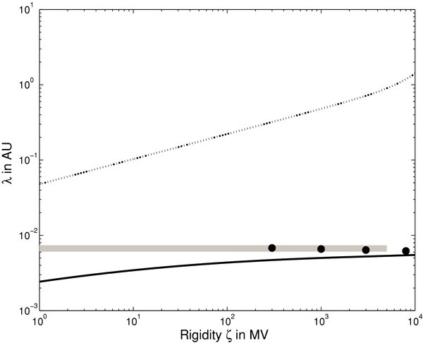
Figure 8. Interplanetary proton transport: the diffusion coefficients vs. the magnetic rigidity in physical units. To obtain these results we have employed the correlation tensor of CLV02. For the parallel diffusion coefficient we have used the quasilinear formula. Shown is the parallel mean free path (dotted line) and the perpendicular mean free path (solid line). The theoretical results are compared with those derived from solar wind observations. Shown is the value suggested by Palmer (1982, gray line) and the value derived by Burger et al. (2000, dots).
Download figure:
Standard image High-resolution image
Figure 9. Interplanetary proton transport: the ratio λ⊥/λ∥ vs. the magnetic rigidity in physical units (solid line). To obtain these results we have employed the correlation tensor of CLV02. For the parallel diffusion coefficient we have used the quasilinear formula.
Download figure:
Standard image High-resolution image
The application of SQLT to compute the diffusion coefficient is questionable. Although for the considered particle energies/rigidities the magnetostatic approximation can be used, it is unclear whether quasilinear theory is valid. There are indications that 2D modes can scatter particles due to nonlinear effects (see Shalchi et al. 2004); there are newer investigations showing that this scattering could be subdiffusive (see Shalchi et al. 2008). In any case, SQLT as used here agrees approximately with solar wind observations and can, therefore, be used for our estimations of perpendicular diffusion coefficients.
In Figure 8, we have compared our theoretical results with two values for λ⊥ obtained from solar wind observations. One value was obtained from Ulysses measurements of Galactic protons (Burger et al. 2000). The second value had been suggested by Palmer (1982) who concluded that the average perpendicular diffusion coefficient at 1 AU heliocentric distance is κ⊥ c/v ≈ 1021 cm2 s−1 corresponding to λ⊥ ≈ 0.0067 AU. Although this quite good agreement between theory and observations is impressive, one should note that it has been achieved previously using standard NLGC theory in combination with the slab/2D model (see Bieber et al. 2004; Shalchi et al. 2006). The new results shown here, however, are based on an improved theory for cross-field scattering and a magnetic correlation tensor which is based on the Goldreich–Sridhar spectrum.
6. SUMMARY AND CONCLUSION
In previous years, much progress has been achieved in the theoretical description of cosmic ray scattering (for a review see, e.g., Shalchi 2009b). Advanced theories for transport across the mean magnetic fields are based on nonlinear methods. In previous work, these theories have been used to describe particle transport and diffusive shock acceleration in the interplanetary system (see, e.g., Zank et al. 2000, 2004, 2006; Bieber et al. 2004; Shalchi et al. 2006, 2010).
In the present paper, we have started to investigate cross-field transport of cosmic rays in the ISM. Our work is based on the improved version of the NLGC theory developed by Shalchi (2010). Like the original NLGC theory proposed by Matthaeus et al. (2003), the new approach requires knowledge of the turbulence properties described by the magnetic correlation tensor  as well as the parallel mean free path λ∥. In the present paper, we have employed two models for the tensor
  , namely,
- 1.The model of CLV02 which is based on the Goldreich & Sridhar (1995) scaling.
- 2.The two-component model which was used previously to approximate solar wind turbulence.
The first model was used by Yan & Lazarian (2002, 2004, 2008) to describe parallel scattering by using quasilinear and nonlinear theories. The second model has been developed to describe parallel and perpendicular diffusion in the solar system (see, e.g., Bieber et al. 1994, 2004; Shalchi et al. 2006).
Another essential ingredient in theories for cross-field scattering is the parallel mean free path. In the present paper, we have tested three different models to replace the parallel diffusion coefficient in our integral equation for the perpendicular diffusion coefficient, namely,
- 1.the Bohm limit, defined as λ∥ = RL,
- 2.the result obtained by employing SQLT,
- 3.the phenomenological model suggested by Büsching & Potgieter (2008).
It is important here to note that for the different models we have a different rigidity dependence of the parallel mean free path. By assuming the form λ∥ ∼ Rν, we find ν = 1 for Bohm diffusion, ν = 1/3 for standard QLT and R < 1, and we have ν = 0.6 in the phenomenological model. The latter rigidity dependence has been reproduced theoretically by Shalchi & Schlickeiser (2005). The three models are compared with each other in Figure 1.
By combining the different turbulence models with the different analytical forms of the parallel mean free path, we have computed the perpendicular mean free path as well as the ratio λ⊥/λ∥. The results obtained for the different models are presented in Figures 2–9. We find the following results.
- 1.
- 2.According to Figures 4 and 5, we find very extreme values if we assume Bohm diffusion. As shown by Figure 1, the Bohm diffusion coefficient does not agree with the phenomenological model. It seems that the assumption of Bohm diffusion is not appropriate in descriptions of particle propagation in the Galaxy and in the solar system.
- 3.As shown in Figure 4, the difference between perpendicular diffusion coefficients calculated by using the phenomenological and the quasilinear diffusion coefficient is small. If we compute the ratio λ⊥/λ∥ we find a discrepancy.
- 4.For interstellar turbulence and particle parameter values, we find that the perpendicular diffusion coefficient is much smaller than the parallel diffusion coefficient (see Figures 6 and 7). The perpendicular diffusion coefficient is approximately κ⊥ ≈ 10−3–10−2(kpc)2 Myr−1 and becomes nearly constant for high rigidities. To obtain these results we employed the phenomenological model to replace the parallel diffusion coefficients in our equations. Furthermore, we find for the ratio of the two diffusion coefficients κ⊥/κ∥ ≈ 10−4–10−1.
- 5.To complement previous work (e.g., Shalchi et al. 2006), we have revisited cross-field transport in the solar system. For the first time we have computed the perpendicular mean free path and the ratio λ⊥/λ∥ for a magnetic correlation tensor which is based on the Goldreich–Sridhar spectrum (see Figures 8 and 9). We find λ⊥/λ∥ ≈ 0.005–0.05 and λ⊥ ≈ 0.006 AU. The latter value is close to the observations of Ulysses measurements of Galactic protons (Burger et al. 2000) and the value suggested by Palmer (1982) who concluded an average perpendicular diffusion coefficient at 1 AU of κ⊥ c/v ≈ 1021 cm2 s−1 corresponding to λ⊥ ≈ 0.0067 AU.
A.L. acknowledges the NSF Grant 08081118, NASA Grant NNX09AH78G, and the NSF-funded Center for Magnetic Self-Organization, as well as an Alexander von Humboldt Award. R.S. thanks the Deutsche Forschungsgemeinschaft (grant Schl 201/19-1) for support. I.B. thanks the 'Galactocauses' project (FI 706/9-1) funded by the Deutsche Forschungsgemeinschaft.
Footnotes
- 4
Whether the independence of the properties of magnetic fluctuations of the particular properties of driving is a valid assumption should be decided considering the problem at hand. If we are concerned with the properties of Alfvénic fluctuations, this means that the coupling between them and the compressible fluctuations should be weak and the inertial range should be long enough for the fluctuations to get into asymptotic regime. The first property, namely weak coupling, was tested in Cho & Lazarian (2002), while the second property, namely the point at which the asymptotic regime is reached, depends on whether turbulence is balanced or imbalanced (see discussion in Beresnyak & Lazarian 2009a).
- 5
The original GS95 work also uses closure relations which are true only in the global frame of reference. The importance of the local system of reference for the GS95 model is first discussed in Lazarian & Vishniac (1999). It is only in the local frame that the critical balance relations are valid.
- 6
- 7
- 8
- 9
Note: there is a misprint in Equation (26) of Yan & Lazarian (2008). The correct formula is D⊥ ≈ 1/3LvE4B or κ⊥ ≈ 1/3lvE4B in the notation used in the present paper.