


ABSTRACT
We present an analysis of the star formation history (SFH) of the transition-type (dIrr/dSph) Local Group galaxy LGS-3 (Pisces) based on deep photometry obtained with the Advanced Camera for Surveys onboard the Hubble Space Telescope. Our observations reach the oldest main-sequence turnoffs at high signal to noise, allowing a time resolution at the oldest ages of σ ∼ 1.1 Gyr. Our analysis, based on three different SFH codes, shows that the SFH of LGS-3 is dominated by a main episode ∼11.7 Gyr ago with a duration of ∼1.4 Gyr. Subsequently, LGS-3 continued forming stars until the present, although at a much lower rate. Roughly 90% of the stars in LGS-3 were formed in the initial episode of star formation. Extensive tests of self-consistency, uniqueness, and stability of the solution have been performed together with the IAC-star/IAC-pop/MinnIAC codes, and these results are found to be independent of the photometric reduction package, the stellar evolution library, and the SFH recovery method. There is little evidence of chemical enrichment during the initial episode of star formation, after which the metallicity increased more steeply reaching a present-day value of Z ∼ 0.0025. This suggests a scenario in which LGS-3 first formed stars mainly from infalling fresh gas, and after about 9 Gyr ago, from a larger fraction of recycled gas. The lack of early chemical enrichment is in contrast to that observed in the isolated dSph galaxies of comparable luminosity, implying that the dSphs were more massive and subjected to more tidal stripping. We compare the SFH of LGS-3 with expectations from cosmological models. Most or all the star formation was produced in LGS-3 after the reionization epoch, assumed to be completed at z ∼ 6 or ∼12.7 Gyr ago. The total mass of the galaxy is estimated to be between 2 and 4 × 10⁸ M☉ corresponding to circular velocities between 28 km s−1 and 36 km s−1. These values are close to but somewhat above the limit of 30 km s−1 below which the UV background is expected to prevent any star formation after reionization. Feedback from supernovae (SNe) associated with the initial episode of star formation (mechanical luminosity from SNe Lw = 5.3 × 1038 erg s−1) is probably inadequate to completely blow away the gas. However, the combined effects of SN feedback and UV background heating might be expected to completely halt star formation at the reionization epoch for the low mass of LGS-3; this suggests that self-shielding is important to the early evolution of galaxies in this mass range.
Export citation and abstract BibTeX RIS
1. INTRODUCTION
The present paper is part of the Local Cosmology from Isolated Dwarfs (LCID)13 project. The Hubble Space Telescope (HST) has been used to obtain deep photometry of six isolated dwarf galaxies in the Local Group: IC 1613, Leo A, Cetus, Tucana, LGS-3, and Phoenix. Color–magnitude diagrams (CMDs) reaching the oldest turn-off points have been derived. The Advanced Camera for Surveys (ACS; Ford et al. 1998) has been used to observe the first five, while Phoenix was observed with the Wide Field and Planetary Camera-2. The main goal of the LCID project is to derive the star formation history (SFH), age–metallicity relation (AMR), and stellar population gradients of this sample of galaxies. Our objective is to study their evolution at early epochs and to probe effects of cosmological processes, such as the cosmic UV background subsequent to the onset of star formation in the universe or physical processes such as the gas removal by supernovae (SNe) feedback. Our sample consists of field dwarfs which were chosen in an effort to study systems as free as possible from environmental effects due to strong interactions with a host, massive galaxy. The SFH is a powerful tool to derive fundamental properties of these systems and their evolution, but to study the earliest epochs of star formation, deep CMDs, reaching the oldest main-sequence turnoffs, are required.
Here we present our analysis of LGS-3. LGS-3 is a dIrr/dSph low-luminosity galaxy discovered by Karachentseva (1976). From its location, it appears to be a member of the Andromeda subgroup of the Local Group (van den Bergh 2000). The distance to the galaxy has been estimated by several authors. Lee (1995), Tikhonov & Makarova (1996), Mould (1997), and Aparicio et al. (1997) used the tip of the red giant branch (TRGB) to estimate distances ranging from 0.6 to 0.96 Mpc. This measurement is inherently challenging because the TRGB region of LGS-3 is very sparsely populated. Miller et al. (2001) also used the TRGB but complemented with observations of the horizontal branch (HB), the red clump (RC), and the overall match of the CMD to model CMDs to estimate a distance of 0.62 ± 0.02 Mpc. Finally, from a study of the RR Lyr stars in LGS-3, Bernard (2009) derived a distance of 0.65 ± 0.05 Mpc ((m − M)0 = 24.07 ± 0.15 mag). We will assume this value in this paper.
The stellar content of LGS-3 has been studied by Lee (1995), Mould (1997), Aparicio et al. (1997), and Miller et al. (2001). Mould (1997) discovered the first Cepheid variable candidates in this galaxy. These works show that LGS-3 contains stars of all ages; it has been forming stars since at least 12 Gyr ago and shows a low recent star formation rate (SFR; Aparicio et al. 1997). The SFH shows a dependency with radius (Miller et al. 2001).
No H ii regions have been found in the galaxy (Hodge & Miller 1995), which is consistent with the low recent star formation activity. The metallicity of the stars has been estimated from the color of the red giant branch (RGB). In this way, Lee (1995) obtained a mean metallicity of ![$\rm [Fe/H]=-2.10\, \pm \, 0.22$](https://content.cld.iop.org/journals/0004-637X/730/1/14/revision1/apj382201ieqn1.gif) , while Aparicio et al. (1997) derived a metallicity range
, while Aparicio et al. (1997) derived a metallicity range ![$\rm -1.45\le [\rm M/H]\le -1.0$](https://content.cld.iop.org/journals/0004-637X/730/1/14/revision1/apj382201ieqn2.gif) . Miller et al. (2001) derived
. Miller et al. (2001) derived ![$\rm [Fe/H]=-1.5\pm 0.3$](https://content.cld.iop.org/journals/0004-637X/730/1/14/revision1/apj382201ieqn3.gif) for the stars older than 8 Gyr, and
for the stars older than 8 Gyr, and ![$\rm [Fe/H]\sim -1$](https://content.cld.iop.org/journals/0004-637X/730/1/14/revision1/apj382201ieqn4.gif) for the most recent generation of stars.
for the most recent generation of stars.
The H i content of LGS-3 was first studied with single disk spectra by Thuan & Martin (1979) and, more recently, with interferometry by Young & Lo (1997). Using the results by the latter authors and the adopted distance of 0.65 Mpc, the results from Young & Lo (1997) correspond to a total H i mass of  M☉, which corresponds to a total atomic gas mass of 3.8 × 10⁵ M☉ when corrected for helium. They also measured a gas velocity dispersion of 8 km s−1 and negligible rotation at a galactocentric radius of 470 pc. The corresponding virial mass estimate is Mvir = 2.1 × 10⁷ M☉.
In this paper, we present the SFH of LGS-3 obtained from observations with the ACS on the HST. The photometry reaches the oldest main-sequence turnoffs of the galaxy, allowing us to obtain an accurate SFH even for the oldest stellar populations. The structure of this paper is as follows. In Section 2, the observations and data reduction are discussed, the CMD is presented, and the completeness tests are described. In Section 3, we describe many of the details of the IAC-pop/MinnIAC methodology and its application to the LCID program observations. The derived SFH of LGS-3 is presented in Section 4 and is compared with those of other LCID galaxies in Section 5. The consequences of SN-driven winds and cosmic reionization on the SFH of LGS-3 are discussed in Section 6. The main conclusions of the work are summarized in Section 7. Finally, in Appendix A, the uniqueness, self-consistency, stability, and statistical significance of the solution are discussed.
2. OBSERVATIONS AND DATA REDUCTION
The ACS observations of LGS-3 were obtained between 2005 September 12 and 17. The F475W and F814W bands were selected as the most efficient combination to trace age differences at old ages, since they provide the smallest relative error in age and metallicity in the main-sequence and sub-giant regions. The total integration time was 15,072 s in F475W and 13,824 s in F814W. The observations were organized in six visits of two orbits each, and each orbit was split into one F475W and one F814W exposure. In the first orbit of each visit, exposure times were 1250 and 1147 s, respectively, while in the second orbit they were 1262 and 1157 s, respectively. Dithers of a few pixels between exposures were introduced to minimize the impact of pixel-to-pixel sensitivity variations ("hot pixels") in the CCDs. The observed field of LGS-3 is shown in Figure 1. The core radius of LGS-3 is 0 82 and its optical scale length is 078 (Mateo 1998), so the 34 × 34 format of the ACS covers a substantial fraction of the stars in LGS-3. Table 1 gives a summary of the observations.

Figure 1. LGS-3 observed field. Orientation and scale are marked.
Download figure:
Standard image High-resolution imageTable 1. Summary of Observations
| Date/UT | Exp. Time (s) | Filter |
|---|---|---|
| 2005 Sep 12 16:18:15 | 2512 | F475W |
| 2005 Sep 12 16:42:00 | 2304 | F814W |
| 2005 Sep 14 16:16:02 | 2512 | F475W |
| 2005 Sep 14 16:39:47 | 2304 | F814W |
| 2005 Sep 15 14:38:40 | 2512 | F475W |
| 2005 Sep 15 15:02:25 | 2304 | F814W |
| 2005 Sep 16 13:01:46 | 2512 | F475W |
| 2005 Sep 16 13:25:31 | 2304 | F814W |
| 2005 Sep 17 11:24:47 | 2512 | F475W |
| 2005 Sep 17 11:48:32 | 2304 | F814W |
| 2005 Sep 17 14:36:38 | 2512 | F475W |
| 2005 Sep 17 15:00:23 | 2304 | F814W |
Download table as: ASCIITypeset image
We analyzed the images taken directly from the STScI pipeline (bias, flat-field, and image distortion corrected). Two point-spread function fitting photometry packages, DAOPHOT/ALLFRAME (Stetson 1994) and DOLPHOT (Dolphin 2000), were used independently to obtain the photometry of the resolved stars. Non-stellar objects and stars with discrepant large uncertainties were rejected based on estimations of profile sharpness and goodness of fit. The final photometric lists contain ∼30, 000 stars each. See Monelli et al. (2010b) for more details about the photometry reduction procedures.
Individual photometry catalogs were calibrated using the equations provided by Sirianni et al. (2005). The zero-point differences between the two sets of photometry are ∼0.05 for F475W–F814W and ∼0.03 for F814W. These small differences are typical for obtaining HST photometry with different methods (Hill et al. 1998; Holtzman et al. 2006). In Section 3, we discuss a technique which minimizes the already small impact of these differences in the obtained SFHs.
The CMD of LGS-3 is shown in Figure 2 for the DOLPHOT photometry. Individual stars are plotted in the left panel and density levels are shown in the right panel. The left axis shows magnitudes in the ACS photometric system corrected for extinction. Absolute magnitudes are given on the right axis using the adopted values for the distance modulus ((m − M)0 = 24.07) and extinctions (AF475w = 0.156 and AF814w = 0.079 mag) (Bernard 2009). In the left panel, the lines across the bottom show the 0.25, 0.50, 0.75, and 0.90 completeness levels derived from false star tests (discussed later in this section). Finally, in order to highlight the main features of the CMD, three isochrones from the BaSTI stellar evolution library (Pietrinferni et al. 2004) are also shown in the right panel.

Figure 2. Color–magnitude diagram of LGS-3. In the left panel, individual stars are plotted while the right panel shows star density levels. Star densities bordering the plotted levels run from 8 to 512 stars dmag−2, evenly spaced by factors of two. The left axis shows magnitudes corrected from extinction. The right axis shows absolute magnitudes. A distance modulus of (m − M)0 = 24.07 and an extinction AF475w = 0.156, AF814W = 0.079 have been used. Bottom lines in the right panel show the 0.25, 0.50, 0.75, and 0.90 completeness levels. Three isochrones from the BaSTI stellar evolution library have been overplotted.
Download figure:
Standard image High-resolution imageThe CMD of LGS-3 shown in Figure 2 reaches ∼1.5 mag below the oldest main-sequence turnoff; these observations are ∼2 mag fainter than the deepest CMD previously obtained for this galaxy (Miller et al. 2001). A comparison of the observations with the overplotted isochrones and the presence of an extended HB indicate that a very old, very low metallicity stellar population is present in the galaxy. The gap produced in the HB by the RR Lyrae variables is visible as well as a narrow RGB. The latter is populated by stars all older than 1–2 Gyr and its narrowness is an indication of a low spread in metallicity. The RC can be observed at the red end of the HB. A main sequence (MS) with stars younger than 200 Myr is clearly apparent. Some blue and red core helium-burning stars might also be present above the RC (m814 < 22.3; 0.5 < (m475 − m814) < 1.2). The RGB bump can also be observed at (m475 − m814) ∼ 1.4 and m814 ∼ 23.2 mag. This evolutionary feature may be used as an indicator of a dominant coeval stellar population homogeneous in metallicity (Monelli et al. 2010a).
Signal-to-noise limitations, detector defects, and stellar crowding can all impact the quality of the photometry of resolved stars with the resulting loss of stars, changes in measured stellar colors and magnitudes, and systematic uncertainties. To characterize these observational effects, we have used the standard technique of injecting a list of false stars in the observed images and obtaining their photometry in an identical manner as for the real stars. These observational effects must be simulated in the stars of the global, synthetic CMD (sCMD, hereafter synthetic stars) to be used for the analysis of the SFH (see below).
Monelli et al. (2010b) provide a detailed description of the procedures we adopt for the characterization and simulation of these observational effects. For the present case of LGS-3, ∼5 × 10⁵ false stars were used for the DOLPHOT photometry and ∼6.5 × 10⁵ were used for the DAOPHOT photometry. The completeness factor, Γ, is defined as the rate of recovered to injected stars as a function of magnitude and color. Figure 2, right panel, shows Γ = 0.25, 0.50, 0.75, and 0.90 for the DOLPHOT photometry. Results for DAOPHOT are similar. At the magnitude level of the oldest MS turn-off stars, Γ ∼ 0.90, allowing for very strong constraints on the oldest epochs of star formation.
We simulate the observational effects in the stars of the sCMD with the routine obsersin. It uses the unrecovered false stars and the differences between the injected (mi) and measured magnitudes (mr) of the recovered stars for the simulation (Aparicio & Gallart 1995). Since the density of stars (and thus the amount of crowding) normally varies substantially across the galaxy's field, spatial information has also been taken into account in the completeness test. To do so, first the spatial density distribution of observed stars in LGS-3 is measured. For that, a grid of 100 × 100 pixel size bins is defined, stars are counted in each bin, and the result is smoothed and normalized. This is used as a density probability distribution to assign positions to each synthetic star. Then, for each synthetic star with magnitude ms, a list of the false stars with |mi − ms| ⩽  m; r ⩽ r is created for each filter, where r is the spatial distance between synthetic and false stars and m and r free input searching intervals. If the number of false stars selected in this way, in common to both filters, is <10, the parameters m and r are increased in turn until 10 or more false stars are found. Then, one of them is randomly selected from this list. If that star was unrecovered, the synthetic star is eliminated from the sCMD. If the selected star was recovered and m'i and m'r are its injected and recovered magnitudes in a given filter, then mes = ms + m'i − m'r will be the magnitude of the synthetic star with observational effects simulated. The same is done for both filters.
3. THE IAC METHOD TO SOLVE FOR THE SFH
3.1. Details of the IAC-star, IAC-pop, and MinnIAC Codes
Our analysis of the SFH of LGS-3 and the rest of LCID galaxies is done upon two fundamental requirements: (1) the consistency of the method, in order to obtain SFHs that are readily comparable and (2) the stability and uniqueness of the solution. To accomplish (1), we have adopted the same criterion on the selection of input parameters to derive the SFH for all galaxies of the LCID project. For (2), we have further developed our method and created new tests and control procedures. Details are given in the following and Appendix A.
The IAC method to solve the SFH is based in three main codes: (1) IAC-star (Aparicio & Gallart 2004) is used for the computation of synthetic stellar populations and CMDs; (2) IAC-pop (Aparicio & Hidalgo 2009) is the core algorithm for the computation of SFH solutions, and (3) MinnIAC (introduced in Aparicio & Hidalgo 2009, but explained in more detail in this paper) is a suite of routines created to manage the process of sampling the parameter space, creating input data, and averaging solutions. As a summary, Figure 3 shows a data flow diagram for the SFH computation process.

Figure 3. Data flow diagram followed in the LCID project to obtain the SFHs of the galaxies. See the text for details.
Download figure:
Standard image High-resolution imageConsidering that time and metallicity are the most important variables in the problem (see Aparicio & Hidalgo 2009), we define the SFH as an explicit function of both. We will use two definitions, one in terms of the number of formed stars and another in terms of gas mass converted into stars. Formally, ψN(t, Z)dtdZ is the number of stars formed within the time interval [t, t + dt] and within the metallicity interval [Z, Z + dZ], while ψ(t, Z)dtdZ is the mass converted into stars within the same intervals. The relation between ψN(t, Z) and ψ(t, Z) is the average stellar mass at birth. Both can be identified with the usual definitions of the SFR, but as a function of time and metallicity.
Several criteria can be used to grid the CMD. The simplest is to use a uniform grid and count stars within each box. However, not all the regions of the CMD and stellar evolutionary phases contain information about the same quality for the purpose of the SFH derivation. An alternative is to give higher weights to regions with more certain stellar evolutionary phases (such as the main-sequence or the sub-giant branch), regions which are more heavily populated or regions in which the photometry is more accurate. To do so, we have introduced what we call bundles (see Aparicio & Hidalgo 2009, and Figure 4), that is, macro-regions on the CMD that can be subdivided into boxes using different appropriate samplings. The number and sizes of boxes in each bundle determine the weight of that region in the derived SFH. This is an efficient and flexible approach for two reasons. First, it allows a finer sampling in those regions of the CMD where the models are less affected by uncertainties in the input physics. Second, the box size can be increased, and the impact on the solution decreased, in those regions where the small number of observed stars could introduce noise due to small number statistics or where we are less confident of the stellar evolution predictions.

Figure 4. Regions of the CMDs (bundles) used for gridding. Bundles are shown overplotted on the observed CMD (left panel) and on one of the synthetic CMD used as an input model for the SFH derivation (right panel). Quantities in the right panel give the number of bins used to sample each bundle.
Download figure:
Standard image High-resolution imageIAC-pop provides a solution for the input set of data and parameters. It can also provide several solutions for the same set by changing the initial random number generator seed. Alternatively, it can deliver several solutions by randomly changing the input data Oj (the number of stars in the original, oCMD, boxes) according to a Poisson statistic. However all of these solutions are eventually sensitive to several other input functions and parameters. To better analyze their effects, we can divide them into four groups. The first group consists of sampling parameters; the main ones are the number and boundaries of parent, pCMDs, and the criteria to define the bundles and grid arrays for sampling the CMDs. The second group consists of external parameters; these are the photometric zero points, distance modulus, and reddening. The third group consists of model functions, which are those functions defining the sCMD; the main ones are the initial mass function (IMF), ϕ(m), and the function accounting for the frequency and relative mass distribution of binary stars, β(f, q) (see Aparicio & Hidalgo 2009). Finally, we have the external libraries, which consist of stellar evolution and bolometric correction libraries. Limiting and measuring the effects of all these parameters in the SFH solution requires several thousand runs of IAC-pop using different input sets. MinnIAC is used to test for the effects of the four groups are treated separately. In general, the solutions obtained with varying sampling parameters are averaged; their rms deviation is also a good estimate of the solution internal error. As for the external parameters and model functions, the set with the best χ2ν is usually adopted. Regarding the external libraries, the solution with the best χ2ν may be adopted, but all the solutions are usually conserved; their differences can provide an indication of the external uncertainties associated with such libraries.
MinnIAC (from Minnesota and IAC) is a suite of routines developed specifically to manage the process of selection of sampling parameters, creating input data sets, and averaging solutions. More in detail, regarding the parameter selection and data input, MinnIAC is used for two tasks. First, to divide the sCMD in the corresponding pCMD according to the selected age and metallicity bins. Second, to define the bundles and box grids in the CMDs and counting stars in them. With this information, MinnIAC creates the input files for each IAC-pop run. Several selections of both simple populations and bundle grids are used within each SFH solution process. MinnIAC does this task automatically, requiring only the input of bundles and corresponding grid sizes, age and metallicity bin sizes, and the steps by which the starting points of the CMD grid as well as age and metallicity bins should be modified from one IAC-pop run to another. A second module of MinnIAC is used to average single solutions found by IAC-pop as required.
3.2. Solving Procedure, Results, and Uncertainties for LGS-3
In this section, we will describe with some details the specific application of the IAC method to the case of LGS-3, detailing the different effects mentioned in Section 3: sampling parameters, external parameters, model functions, and external libraries. Our choices are summarized in Table 2. For each item, Columns 2, 3, and 4 give minimum (or choice 1), maximum (or choice 2), and the step used (if relevant), respectively. Column 5 gives the final adopted value (if relevant). The SFH of LGS-3 has been derived independently for the DOLPHOT and DAOPHOT photometry sets following the same procedure as described below.
Table 2. Functions and Parameters Tested and Adopted for the SFH
| Function/Parameter | Min. Value | Max. Value | Step | Adopted |
|---|---|---|---|---|
| Stellar evolution library | BaSTI | Girardi | ⋅⋅⋅ | BaSTI |
| Binary fraction | 0.0 | 1.0 | 0.2 | 0.4 |
| IMF (0.1 ⩽ m ⩽ 0.5 M☉)a | 0.0 | 4.0 | 0.1 | 1.3 |
| IMF (0.5 < m ⩽ 100 M☉) | 0.0 | 5.0 | 0.1 | 2.3 |
| ΔZF475Wb | −0.21 | 0.21 | 0.105 | 0.13/0.08 |
| ΔZF814Wb | −0.15 | 0.15 | 0.075 | 0.11/0.11 |
| CMD griddingc,d | 0.01 × 0.2 | 0.01 × 0.2 | ⋅⋅⋅ | ⋅⋅⋅ |
Age sampling ( )d )d |
0.2 Gyr | 0.5 Gyr | ⋅⋅⋅ | ⋅⋅⋅ |
Age sampling ( ) ) |
1.0 Gyr | 1.0 Gyr | ⋅⋅⋅ | ⋅⋅⋅ |
| Metallicity sampling (Z ⩽ 0.001)d | 0.0002 | 0.0002 | ⋅⋅⋅ | ⋅⋅⋅ |
| Metallicity sampling (Z>0.001) | 0.0005 | 0.0005 | ⋅⋅⋅ | ⋅⋅⋅ |
Notes. aValues are the exponent x in the IMF defined as ϕ(m) = Am−x, where m is the mass and A is a normalization constant. bZero-point offsets are relative to Sirianni et al. (2005). The adopted values were selected by interpolation. Results for DOLPHOT/DAOPHOT are given in the last column. cValues are the box size (color × magnitude) for the CMD sampling. dSeveral bin sets were tested using the same bin size but applying different offsets to the starting point of the bin set.
Download table as: ASCIITypeset image
Using IAC-star, several sCMDs were computed, one with each of the IMFs and binarity functions listed in Table 2. Each sCMD was built with 8 × 10⁶ stars with a constant SFR in the range of age 0–13.5 Gyr and a metallicity range 0.0001–0.005. The latter value has been assumed after a preliminary test with isochrones which showed that stars with metallicity larger than 0.005 do not exist in LGS-3. Using a large number of synthetic stars in the sCMD is important in order to minimize the stochastic effects of the Monte Carlo simulations used in IAC-star, to have a statistically significant number of stars in each pCMD (>6000 stars), and to reduce the uncertainties in the stellar composition of simple populations in the pCMDs.
The bundles and one of the grid sets used to bin the CMDs are shown in Figure 4. In total, 72 combinations of IMF and binarity (model functions) have been tested. For each of them, 24 solutions have been obtained by varying the CMD binning and the simple stellar population sampling (sampling parameters). The average  of these 24 solutions is adopted as the solution for the specific IMF and binarity. These averages have been obtained by using a boxcar of width 1 Gyr and step 0.1 Gyr for t and width 0.0006 and step 0.0001 for Z. A
  is also obtained as the average of the 24 single χ2ν values. The average solution with the smallest
  is assumed as the best one. The IMF and the binary fraction corresponding to this solution are assumed here as the ones best representing our photometry data, although we do not intend to reach any strong conclusions concerning their true values.
To minimize the effects of external parameters (distance, reddening and photometry zero point), the SFH is derived for different offsets in color and magnitude applied to the oCMD. The offset giving the minimum  is assumed as the best. These are obtained when the oCMD is shifted by [Δ(F475W−F814W), Δ(F814W)] = [0.02, 0.11] and [ − 0.03, 0.11] for the DOLPHOT and DAOPHOT photometry sets, respectively. These tests also provide a way to estimate how distance, reddening, and zero-point uncertainties translate into the solution of the SFH. Defining
  as the
  value of the best solution, if
  is its corresponding rms deviation, all the solutions with
  should be considered valid. We can assume that the rms deviation of all the corresponding single solutions is a proxy of the error of the adopted solution, σP.
The former error, σP, includes the effects of sampling and external parameters. However, there is one more source of uncertainty that must be taken into account, namely, the effect of statistical sampling in the oCMD. To estimate this, the solution is again obtained after varying the numbers of stars in the oCMD grid according to a Poisson statistic. This is done 20 times and the rms deviation of the solutions, σI, is obtained. The final adopted error is the sum in quadrature σSFH = (σ2I + σ2P)1/2.
Finally, solutions have been obtained using both the BaSTI (Pietrinferni et al. 2004) and the Girardi et al. (2000) stellar evolutionary libraries (external libraries). In both cases, the bolometric corrections by Bedin et al. (2005) were used. Both produced qualitatively similar results, and a comparison between them together with the results obtained with other methods is presented in Section 4.3. For detailed analysis presented in the following sections, for simplicity, we use only the BaSTI stellar evolutionary libraries.
4. THE SFH OF LGS-3
4.1. Main Features of the SFH of LGS-3
Figure 5 shows plots of the SFH of LGS-3, ψ(t, Z), as a function of both t and Z derived from the two different photometry sets. ψ(t) and ψ(Z) are also shown in the ψ − t and ψ − Z planes, respectively. The projection of ψ(t, Z) on the age–metallicity plane shows the AMR, including the metallicity dispersion.

Figure 5. Star formation history, ψ(Z, t), of LGS-3 obtained from DOLPHOT (upper panel) and DAOPHOT (lower panel) photometry sets. The SFH as a function of age ψ(t) and metallicity ψ(Z) are shown projected on the ψ–time and ψ–metallicity planes, respectively. Dashed lines give the error intervals. The age–metallicity relationship is the projection onto the look-back time–metallicity plane.
Download figure:
Standard image High-resolution imageIn Figure 6 we show ψ(t), the AMR, and the cumulative mass fraction of LGS-3 as a function of time with their associated errors. Three vertical dashed lines show the ages of the 10th, 50th, and 95th percentiles of the integral of ψ(t). Table 3 gives a summary of the integrated and mean quantities for the observed area and estimates for the whole galaxy.

Figure 6. ψ(t) (upper panel), metallicity (middle panel), and cumulative mass fraction (lower panel) of LGS-3 obtained from DOLPHOT (thick, solid lines) and DAOPHOT (thick, dashed lines) photometry sets. Thin lines give the uncertainties. Cyan lines show the final adopted solution, which is the mean of DOLPHOT and DAOPHOT ones. Vertical dotted-dashed lines indicate the times corresponding to the 10th, 50th, and 95th percentiles of ψ(t), i.e., the times for which the cumulative fraction of mass converted into stars were 0.1, 0.5, and 0.95 of the current one. A redshift scale is given in the upper axis, computed assuming  , Ωm = 0.273, and a flat universe with ΩΛ = 1 − Ωm.
Download figure:
Standard image High-resolution imageTable 3. Summary of Integrated and Mean Quantities of the LGS-3 SFH
| Area (kpc2) | Mass Formed (106 M☉) | 〈[M/H]〉 | 〈ψ(t)〉(10−3 M☉ yr−1) |
|---|---|---|---|
| 0.42 | 1.26 ± 0.04 | −1.7 ± 0.1 | 0.09 ± 0.03 |
| Total Galaxy | 1.95 ± 0.04 | −1.7 ± 0.1 | 0.14 ± 0.03 |
Download table as: ASCIITypeset image
The main features of the SFH of LGS-3 can be observed in Figure 6. The bulk of the star formation of LGS-3 occurred at old epochs, with a main peak located ∼11.5 Gyr ago. The initial episode of star formation lasted until roughly 9 Gyr ago. Approximately 85% of the stars were formed in this initial episode. Since then, the SFR has been very low and slowly declining until the present. The SFR at the measured main peak is a factor of 15 larger than the mean SFR between 0 and 9 Gyr ago (because of limited time resolution, this is a lower limit, see Section 4.2). It is worth noting that the age at which the rate of the AMR starts to increase more steeply matches up with the age at which the SFR decreases to a low level. This may indicate a scenario in which the stars were formed at a higher rate at old epochs from fresh, low-metallicity gas. When the initial episode of star formation was over, the gas reservoir would have been nearly exhausted. As a consequence, subsequent star formation would occur at a much lower rate and from an ISM including a high fraction of processed gas, hence significantly increasing the metallicity enrichment rate.
It is interesting to test whether the number of SNe produced in LGS-3 during its lifetime is sufficient to produce the chemical enrichment we have derived. Focusing on the main episode, 1.7 × 10⁶ M☉ of gas was converted into stars from 13.5 to 8.5 Gyr ago. Assuming a minimum progenitor mass for core collapse SNe of 6.5 M☉ (Salaris & Cassisi 2005) we obtain a total of 2.9 × 10⁴ SNe produced in the old episode. Accounting for stellar mass loss and assuming a minimum initial mass of 10 M☉ for SNe progenitors, the total number of SNe decreases to 1.6 × 10⁴. This can be compared to an estimate of the total number of SNe necessary to produce the observed chemical enrichment. Assuming the solar abundance distribution from Grevesse & Noels (1993), that only Type II supernovae (SNe II) are involved, and using the iron mass production rate from Nomoto et al. (1997) (see Monelli et al. 2010c, for more details), we estimate that ∼80 SNe II are enough to produce an increment of metallicity from 0 to 0.0007, which is the upper value obtained for LGS-3 8.5 Gyr ago. This estimate was derived assuming the iron mass production of a 13 M☉ star (which may vary by a factor of 2–3 with different assumptions). Although relatively uncertain, our calculation shows that the galaxy needs to retain only roughly 1% of the material released by SNe in order to produce the observed metallicity increase. The same calculation can be made for the chemical evolution from 8.5 Gyr ago to the present. In this case, the mass of gas converted into stars is 2.4 × 10⁵ M☉ and the corresponding numbers of SNe are 4.1 × 10³ and 2.4 × 10³. In this time, the metallicity increases from Z = 0.0007 to a current upper value of Z = 0.003, requiring 290 SNe. This is less than 15% of the total, a much larger fraction than calculated for the initial star formation episode. This implies that a significantly larger fraction of the newly synthesized material was captured at later times at lower SFRs. Note that only SNe II have been considered for this estimate; if Type Ia supernovae (SNe Ia) were also included, even lower fractions of captured newly synthesized material would result. Note also that much of the latter enrichment could be achieved by SNe Ia from the initial star formation episode.
The SFH shown in Figure 6 corresponds to the observed area, which covers the center and a major fraction of the galaxy. The total mass of stars created in this area over the lifetime of the galaxy is 2.0 × 10⁶ M☉. Assuming an exponential density distribution of scale length 112 pc (S. Hidalgo et al. 2011, in preparation), we estimate that the total mass of stars ever formed in LGS-3 is 1.1 × 10⁶ M☉. Adding in the gas mass (Young & Lo 1997, see Section 1), the total baryonic mass of LGS-3 is 1.5 × 10⁶ M☉. These values correspond to the best solution with the adopted IMF (x = 1.3 for the interval 0.1 ⩽ m ⩽ 0.5 M☉; x = 2.3 for the interval 0.5 ⩽ m ⩽ 100 M☉; see Table 2). If a Salpeter IMF with an exponent of 2.35 for the range 0.1–100 M☉ is used, then the result would be larger by a factor of ∼1.5.
Figure 7 shows the observed CMD, the best-fit CMD, and the corresponding residuals. The calculated CMD has been built using IAC-star with the solution SFH of LGS-3 as input. Residuals are given in units of Poisson uncertainties, obtained as  , where noi and nci are the numbers of stars in bin i of a uniform grid defined on the observed and calculated CMDs, respectively.

Figure 7. Observed (left panel), calculated (central panel), and residuals (right panel) CMDs. The calculated CMD has been built using IAC-star with the solution SFH of LGS-3 as input. The gray scale and dot criteria for the first two are the same as for Figure 2. The residuals are in units of Poisson uncertainties.
Download figure:
Standard image High-resolution image4.2. Estimating the Effects of Time Resolution on the SFH
Observational uncertainties as well as the uncertainties inherent to the SFH computation procedure result in a smoothing of the derived SFH and a decrease of the age resolution (see Appendix A.3). Having an accurate estimate of this age resolution is fundamental in order to obtain reliable information of the actual properties of the galaxy. We have calculated the age resolution as a function of time by recovering the SFH of a set of mock stellar populations corresponding to very narrow bursts occurring at different times. Five mock populations have been computed, each one with a single burst at ages of 1, 4, 8, 11.5, and 13 Gyr. We used IAC-star to create the CMDs associated with each mock stellar population. For the mock populations at ages of 11.5 and 13 Gyr, five simulations have been done with different random number seeds in order to better characterize them. The assumed metallicities and SFRs correspond to those obtained for LGS-3. Observational uncertainties were simulated in the CMDs by using the results of the DOLPHOT completeness tests. The SFHs of the mock stellar populations were then obtained using the identical procedure as for the real data. In all cases, the recovered SFH is well fitted by a Gaussian profile with σ depending on the burst age. Figure 8 shows the input bursts and the corresponding Gaussian profile fits to the solutions, including their peak age and σ. From these results, we estimate an intrinsic age resolution of ∼1.1 Gyr at the oldest ages which decreases to ∼0.5 Gyr at an age of 1 Gyr. Also, a slight shift is observed between the input and solution ages. For the oldest trials, the shift is toward younger ages (up to 0.4 Gyr for the oldest trial) and for the youngest trials it is toward older ages (about 0.2 Gyr).

Figure 8. Results of the tests of time resolution. Arrows indicate the burst age of the simulated populations. Bursts have a duration of 105 M☉ and their intensities are similar to the SFR of LGS-3 at the corresponding age. The heights of the arrows are not indicative of burst intensity. Curves show the Gaussian profile fits to the solutions. The Gaussian profile areas are normalized to the same value for easier comparison. The solution peaks (μ) and standard deviations (σ) are given.
Download figure:
Standard image High-resolution imageIt is particularly important to determine the oldest age at which star formation occurred in LGS-3 and the real duration of the first, main star formation episode. Our SFH solution (Figure 6) is well fitted by a Gaussian profile with a peak, μobs = 11.5 Gyr and σobs = 1.2 Gyr in the age range 9.5–13.5 Gyr (using the DOLPHOT photometry). The shifts shown in Figure 8 indicate that the actual star formation peak would have occurred at about 11.7 Gyr ago. A comparison of the solution with our estimated resolution indicates that the initial episode of star formation is just barely resolved in our observations. A quadratic subtraction of σ ∼ 1.1 that we have obtained for a sharp burst at this age from the derived σobs = 1.2 provides a first estimate of the actual, intrinsic dispersion of σreal ∼ 0.5.
Given the importance of this measurement, we have pursued a more detailed analysis. We have extended the former tests to a set of mock stellar populations with SFHs defined as Gaussian profile shaped bursts of different σ and centered at 11.5 Gyr. Observational uncertainties were simulated in the associated CMDs and the SFHs were recovered following the same process as for the galaxy. In all cases, the recovered SFHs are well fitted by Gaussian profiles in the age range 9.5–13.5 Gyr. Figure 9 shows a quadratic fit to the standard deviation of the solutions, σmockrec, as a function of the input ones, σmockin. If the actual LGS-3 SFH were well described as a Gaussian profile, its σ could be inferred by interpolating in this fit, which gives σobsin = 0.6 Gyr. We will adopt this value for the forthcoming discussion.

Figure 9. Standard deviation, σmockrec, of Gaussian profile fit solutions obtained for a set of Gaussian profile mock input SFHs with standard deviation σmockin, centered at about the age of the peak of the main episode of LGS-3 (11.5 Gyr). Observational uncertainties were simulated in the associated mock CMDs, and the SFHs were recovered following the same procedure as for LGS-3. A quadratic fit to the data is shown, together with the σ value measured in the real data solution (σobsrec) and the corresponding real value inferred using the fit (σobsin).
Download figure:
Standard image High-resolution image4.3. Comparison with Other SFHs Derivation Methods
As for the rest of the LCID galaxies, we have obtained the SFH of LGS-3 using the Match (Dolphin 2002) and Cole (Skillman et al. 2003) methods in addition to the IAC method. These two methods use Girardi et al. (2000) for the stellar evolution library, and we have adopted the DOLPHOT photometry to be used with them for this comparison (for a description of the main features of these methods and the particulars of their application to LCID galaxies, see Monelli et al. 2010b). For a proper comparison, we have also obtained the SFH with IAC-star/MinnIAC/IAC-pop using the same library and photometry. This also allows us to compare the solutions obtained with the IAC method using two different stellar evolution libraries.
Figure 10 shows the cumulative mass fraction of LGS-3 as obtained with the three tested methods. The agreement between the three methods resulting in the same cumulative mass fraction (0.8) at 8 Gyr is very good. This strongly supports the conclusion that the majority of the star formation in LGS-3 occurred during this initial episode of star formation. Also, all three methods find star formation continuing at much lower rates, until the present. The similar behavior of the three solutions allows us to be confident that our scientific conclusions are independent of the SFH solution method. In particular, the fact that the galaxy has formed most of the stars after the reionization epoch is also confirmed and even reinforced.

Figure 10. Cumulative mass fraction as a function of look-back time of the solutions obtained for LGS-3 with different methods indicated in the label. All of them use the DOLPHOT photometry. IAC-B corresponds to the solution adopted and discussed in this paper, obtained with IAC-star/MinnIAC/IAC-pop using the BaSTI stellar evolution library. IAC-G has been obtained with IAC-star/MinnIAC/IAC-pop but using the Girardi et al. (2000) stellar evolution library. Cole and Match methods make use of the Girardi et al. (2000) stellar evolution library.
Download figure:
Standard image High-resolution imageFigure 10 also shows the effect of using different stellar models by comparing the IAC-star/MinnIAC/IAC-pop results using two different stellar libraries. Here, we see that the SFH derived using the BaSTI stellar evolution library has a slightly faster rise compared to the SFH derived using the Girardi et al. (2000) library. However, otherwise, the two are in very good agreement, and the main features of the SFH of LGS-3 are found in both derived models at roughly equivalent levels.
An analysis of the actual resolution provided by the Match and Cole methods of the kind of that done for IAC-star/MinnIAC/IAC-pop in Section 4.2 would be necessary before going deeper in this comparison, which is beyond our objectives here. In the following, we will use only the results obtained with IAC-star/MinnIAC/IAC-pop and the BaSTI stellar evolution library.
5. THE SFH OF LGS-3 COMPARED TO OTHER LCID GALAXIES
In this section, we will compare the SFH of LGS-3 with that of Phoenix (the other dSph/dIrr transition galaxy of the LCID sample; Hidalgo et al. 2009) and with those of Cetus and Tucana (the two dSphs of the sample; Monelli et al. 2010b, 2010c).
Figure 11 shows the SFH and the AMR of LGS-3 compared to those of Phoenix (Hidalgo et al. 2009). The correspondence between the main properties of both galaxies is remarkable. Both galaxies show a dominant period of initial star formation at early times, with a result that both galaxies had formed 50% of their total stellar mass about 10.5–11.0 Gyr ago, or before a redshift of 2. Both galaxies had also formed more than 95% of their total stellar mass by 2 Gyr ago. The AMRs of Phoenix and LGS-3 show similar behavior from the earliest times, with ![$[\rm M/H]\sim -1.7$](https://content.cld.iop.org/journals/0004-637X/730/1/14/revision1/apj382201ieqn18.gif) , until reaching 95% of the cumulative mass fraction, with
, until reaching 95% of the cumulative mass fraction, with ![$[\rm M/H]\sim -1.2$](https://content.cld.iop.org/journals/0004-637X/730/1/14/revision1/apj382201ieqn19.gif) . Note that, in both cases, the slope of the AMR increases about ∼8–9 Gyr ago, after the initial episode of star formation.
. Note that, in both cases, the slope of the AMR increases about ∼8–9 Gyr ago, after the initial episode of star formation.

Figure 11. Comparison between the SFHs and the AMRs of LGS-3 (this paper) and Phoenix (Hidalgo et al. 2009). A redshift scale is given on the top axis, computed assuming  , Ωm = 0.273, and a flat universe with ΩΛ = 1 − Ωm. Vertical dotted-dashed lines indicate the times corresponding to the 10th, 50th, and 95th percentiles of ψ(t) for each galaxy, i.e., the times for which the cumulative fraction of mass converted into stars were 0.1, 0.5, and 0.95 of the current one.
Download figure:
Standard image High-resolution imageThe SFHs of both transition-type galaxies are similar to those of the two dSphs in the sense that an old, main episode exists and that a sharp drop off in the SFR occurred ∼9 Gyr ago. After this, the transition galaxies, Phoenix and LGS-3, were able to form stars at low, steadily decreasing rates while the dSphs completely stopped their star formation. Monelli et al. (2010c) showed that the first, main episode of star formation occurred earlier in Tucana than in Cetus. The main episode of star formation LGS-3 has an age comparable to that of Cetus and is also clearly younger than that of Tucana.
There are significant differences between the AMRs of the transition and the dSph galaxies even for t>9 Gyr. The metal enrichment from the earliest times up to ∼9 Gyr ago is less than 0.1 dex in LGS-3 and Phoenix, while it is more than 0.4 dex in the same period in the dSph galaxies (Monelli et al. 2010b, 2010c). In the case of the transition galaxies, more than 80% of the stars were formed with roughly the same metallicity. This result is supported by the narrow RGB of LGS-3 as described in Section 2, indicative of a low-metallicity spread for the intermediate-to-old age stars.
The differences between the AMRs of the transition and dSph galaxies are intriguing. Galaxy mass is the fundamental parameter which is thought to determine a galaxy's ability to retain gas. This might naively imply that the dSphs were initially more massive systems than the transition galaxies. However, today, Cetus, Tucana, LGS-3, and Phoenix all have comparable luminosities. Tidal stripping is thought to be very important in the evolution of dSph galaxies (see Peñarrubia et al. 2008, and references therein). The comparable present-day luminosities, combined with the difference in AMRs, could point to significantly larger halo masses for the isolated dSphs which have been lost to tides, or, in other words, a much smaller impact of tides on the evolution of the transition galaxies.
6. COSMOLOGICAL CONSIDERATIONS AND THE EARLY EVOLUTION OF LGS-3
6.1. Background
Dwarf galaxies are the focus of a major cosmological problem affecting the CDM scenario; the number of dark matter subhalos around Milky Way-type galaxies predicted by CDM simulations is an order of magnitude larger than observed (Kauffmann et al. 1993; Klypin et al. 1999; Moore 1999). Several explanations have been proposed to solve this problem but most of them use two main processes that can dramatically affect the formation and evolution of dwarf-sized halos: heating from the ultraviolet (UV) radiation arising from cosmic reionization and internal SN feedback. Both are, in principle, capable of stopping the star formation in a dwarf halo and even to fully remove its gas. The detailed information about the SFH at early and intermediate ages, such as we have obtained here, may provide fundamental insight into the problem and help to discriminate between the different scenarios proposed so far. Detailed discussions about this complex problem can be found in Mac Low & Ferrara (1999), Bullock et al. (2001), Stoehr et al. (2002), Kravtsov et al. (2004), Ricotti & Gnedin (2005), Strigari et al. (2008), and Sawala et al. (2010), among others. Here, we will give a short summary just to place our forthcoming discussion in context.
Feedback from SNe can suppress star formation or even blow out the gas completely from the smallest systems. Mac Low & Ferrara (1999) presented detailed models showing that the mass ejection efficiency is low in galaxies with baryonic mass above ∼107 M☉ and that only galaxies with baryonic mass below ∼106 M☉ could have their gas completely blown away almost independently of the SNe mechanical luminosity. It is worth mentioning that, according to the assumptions of Mac Low & Ferrara (1999), a baryonic mass of ∼106 M☉ would correspond to a total mass of 6.8 × 10⁷ M☉, while a baryonic mass of ∼107 M☉ would correspond to 3.5 × 10⁸ M☉.
There is a consensus that UV background heating establishes a characteristic time-dependent minimum mass (a filtering mass) for halos that can accrete gas (e.g., Gnedin 2000; Kravtsov et al. 2004). The UV background will heat the gas in low-mass halos, preventing star formation, and eventually photoevaporate them. As a result, halos not massive enough to have accreted gas before the reionization epoch would fail to do so later, unless they accrete mass faster than the rate at which the filtering mass increases. The redshift of the reionization epoch has been estimated from polarization observations of the CMB to be z = 10.9 ± 1.4 (WMAP 5 year results; Komatsu et al. 2009). However, the presence of the Gunn–Peterson trough in quasars at z ∼ 6 shows that the universe was not yet fully reionized at earlier epochs (Loeb & Barkana 2001; Becker et al. 2001).
According to models (see, e.g., Mac Low & Ferrara 1999), the minimum circular velocity for a dwarf halo to accrete and cool gas in order to produce star formation is vc ∼ 30 km s−1, which corresponds to a total mass of ∼109 M☉. However, most dwarf galaxies in the Local Group, including all the Milky Way satellites and five out of the six of the LCID sample, show circular velocities well below that value. Nevertheless, there are currently several proposed ways to overcome this apparent contradiction. Bullock et al. (2001) have proposed that dSph and the rest of the smallest halos would have been formed during the prereionization era. The processes of photoionization feedback resulted in the suppression of the star formation below an observable level in 90% of them. This was supported by Ricotti & Gnedin (2005), who found that if positive feedback is considered, a fraction of low-mass halos (total mass below 108 M☉) would have been able to form stars before the reionization era. The star formation in these galaxies would have been halted by internal mechanisms, like photodissociation of H2 or SN feedback in advance of the reionization era. Another possibility is that masses of dark matter halos of the dSphs galaxies would be much larger than those measured at the optical limit of the galaxies and larger than the limit required by the reionization scenario (Stoehr et al. 2002). In these scenarios, dark matter halos of lower masses would have failed to form stars and remain dark. Alternatively, dark matter halos could have been much larger in the reionization epoch, with total masses above the mass required for star formation, but they lost a large fraction of their mass afterward due to tidal harassment (Kravtsov et al. 2004). It is also possible that a self-shielding mechanism would be present, protecting the gas in the inner regions or in regions denser than some limit from being heated by the UV background (Susa & Umemura 2004). Finally, it has been suggested that inhomogeneous reionization can lead to large variations in the masses of halos that survive and produce stars (Busha et al. 2010).
In summary, it is useful to note that the first scenario (Bullock et al. 2001; Ricotti & Gnedin 2005) and also the last ones (Susa & Umemura 2004; Busha et al. 2010) allow star formation in low-mass halos (total mass below 108–109 M☉), while the second and third are compatible with star formation in more massive halos only (total mass above 109 M☉). Additionally, the first scenario would imply that star formation would have been produced before reionization and would have been halted afterward in the smallest galaxies.
Recently, Sawala et al. (2010) have presented a set of high-resolution hydrodynamical simulations of the formation and evolution of isolated dwarf galaxies including the most relevant physical effects, namely, metal-dependent cooling, star formation, feedback from Type II and Ia SNe, and UV background radiation. Their results are very useful for a direct comparison with observations. They study halos with present-day total masses between 2.3 × 10⁸ M☉ and 1.1 × 10⁹ M☉ and reach an interesting set of conclusions that include many of the aforementioned ones. First, halos that are not massive enough to accrete sufficient gas to form stars before z = 6 lose their gas subsequently due to UV background heating. In this sense, reionization sets a lower mass limit of the halo for star formation. Second, in halos that form stars, feedback is the main process driving the evolution of the galaxy and regulating its star formation. It alone can blow out all the gas of a dwarf system before z = 0, while UV background alone has almost no effect. However, if feedback has previously made the gas diffuse and reduced its radiative cooling efficiency, then the UV background has a strong effect, producing a sharp cutoff in the star formation at the epoch of reionization. Finally, self-shielding is effective only in the inner regions of the halos at the more massive end.
All the aforementioned mechanisms are founded on solid and extensive theoretical modeling. However to decide to what extent one or another should be preferred, detailed observational evidence is necessary. One such observable is whether the star formation in the smallest galaxies was halted at reionization. To answer this question, a precision of ∼1 Gyr is required in the determination of the SFH at 12.5–13 Gyr ago (Ricotti & Gnedin 2005), which is indeed what we have reached in our work. In the following, we will discuss the different possibilities in light of our results for LGS-3 paying attention first to SN feedback effects and second to UV background effects.
6.2. SN Feedback in LGS-3
The SFH obtained for LGS-3 allows us to make a direct estimate of the importance of feedback in LGS-3. To do so, the mechanical luminosity of the SNe produced in the main star formation episode and the mass of the galaxy can be compared with the results of Mac Low & Ferrara (1999). They used models to calculate the conditions for blow-away, partial mass loss, and no mass loss of dwarf galaxies as a function of the baryonic mass of the galaxy and the mechanical luminosity, Lw, of the SNe produced during a central, instantaneous star formation episode.
The kinetic energy released to the interstellar medium by the SNe produced in the old, main star formation episode in LGS-3 can be computed as follows. For a continuous SFR of 1 M☉ yr−1, the STARBURST99 models (Leitherer et al. 1999) predict a mechanical luminosity of log Lw = 41.9. This is the equilibrium value reached after a few tens of million years from the first star formation. The SFR is for a mass range 1–100 M☉ and is computed using a classical IMF with exponent −2.35. For direct comparison, we convert this rate to the same stellar mass interval and IMF that we have used and obtain 1.7 M☉ yr−1. Scaling these values to the SFR obtained for LGS-3, the total mass converted into stars in the initial episode is 1.7 × 10⁶ M☉. Assuming a Gaussian profile of σ = 0.6 Gyr, or a duration (FWHM) of 1.4 Gyr, results in an average SFR of 1.3 × 10⁻³ M☉ yr−1. Scaling STARBURST99 models to this average SFR results in a mechanical luminosity of Lw = 5.3 × 1038 erg s−1.
Alternatively, we can compute the mechanical luminosity from core collapse SNe only (note that STARBURST99 includes all sources of mechanical luminosity). From Section 3, the total number of SNe formed during the old, main episode was 2.9 × 10⁴ or 1.6 × 10⁴ for minimum core collapse progenitor masses of 6.5 M☉ or 10 M☉, respectively (Salaris & Cassisi 2005). Assuming an energy release per SN of 1051 erg (Leitherer et al. 1999), we obtain a total mechanical luminosity released during the old, main episode of Lw = 6.8 × 1038 erg s−1 or Lw = 3.8 × 1038 erg s−1, respectively. Since these values are compatible with the STARBURST99 estimate, we will adopt Lw = 5.3 × 1038 erg s−1. Combining this with a baryonic mass of 1.5 × 10⁶ M☉ (Section 4.1), the model results of Mac Low & Ferrara (1999) shown in their Figure 1 place LGS-3 in the regime of mass loss, but fairly close to the blow-away regime.
However, Equation (1) from Mac Low & Ferrara (1999) gives a relation between the baryonic and dark matter masses of dwarfs which is an extrapolation to low-mass galaxies of the relation derived by Persic et al. (1996) for more massive galaxies (total masses above 1010 M☉). From this relation, the total mass for LGS-3 is 9 × 10⁷ M☉. Alternately, Sawala et al. (2010) give the final (z = 0) stellar, gaseous, and total masses for their model runs. The relations between these parameters depend on the model ingredients, but for a baryonic mass like that of LGS-3, the total mass is in the range from 2 × 10⁸ M☉ to 4 × 10⁸ M☉. Using this estimate instead of the Persic et al. (1996) extrapolation places LGS-3 well within the regime of mass loss due to feedback and far from the blow-away regime.
6.3. The Effects of Reionization
A flat Einstein–de Sitter universe with  , Ωm = 0.273 (as derived from the WMAP 5 year data; Komatsu et al. 2009), has an age ∼13.7 Gyr. The WMAP 5 year data indicate the epoch of reionization occurred at z ∼ 10.9 corresponding to a look-back time of ∼13.3 Gyr. Evidence from quasar spectra indicates that the epoch of reionization is over at a redshift of z ∼ 6 or a look-back time of ∼12.7 Gyr (Becker et al. 2001). We will focus on the latter since it is more conservative from the point of view of the forthcoming discussion.
Did LGS-3 form most of its stars before or after the epoch of reionization? Using the cumulative mass fraction from Figure 6, we find that more than 80% of the stellar mass of LGS-3 has been formed later than ∼12.5 Gyr ago (z ∼ 5). Thus, the observations indicate that the majority of the stars in LGS-3 were formed after the epoch of reionization.
We can use synthetic data to better assess this constraint. In Figure 12, we show the results of two synthetic SFHs, one in which all stars are formed between 13.4 and 12.4 Gyr ago (before the epoch of reionization) and another where all of the stars are formed between 11.9 and 10.9 Gyr ago. Figure 12 shows that the model where all of the stars formed before the epoch of reionization is clearly inconsistent with the SFH of LGS-3. On the other hand, the model with all stars forming after the epoch of reionization is a good match to our SFH for LGS-3, indicating that it is highly unlikely that LGS-3 formed a large fraction of its stars before reionization had concluded.

Figure 12. SFH obtained for two mock galaxies, compared with the actual SFH of LGS-3. One of the mock galaxies simulates a system in which most or all the star formation occurred before reionization (star formation between 12.4 and 13.4 Gyr ago; gray, vertical lines). The other one simulates a system in which all the star formation occurred after reionization (star formation between 10.9 and 11.9 Gyr ago; black, vertical dotted lines). Gray solid and black dotted lines show the solutions obtained for them while the black solid line corresponds to LGS-3. This figure provides strong evidence that most, if not all, of the star formation in LGS-3 occurred after reionization.
Download figure:
Standard image High-resolution imageHowever, the absolute ages in our comparisons are intrinsically dependent on the stellar evolution models which have intrinsic uncertainties (e.g., Chaboyer 1995; Chaboyer et al. 1998). Modern stellar evolution models have addressed many of the shortcomings in earlier generations of models (e.g., see discussion in Dotter et al. 2007), and the results of the relative ages derived from main-sequence stars are in excellent agreement (better than 0.5 Gyr) as demonstrated by Marín-Franch et al. (2009). The accuracy of the absolute ages is also increasing. For example, the average age of the oldest globular clusters obtained from the age analysis by Marín-Franch et al. (2009), using the BaSTI library, is 12.3 Gyr with an age dispersion of ±0.4 Gyr (A. Marín-Franch 2011, private communication). In this regard, the complete inconsistency of our SFH for LGS-3 with the model in which all stars are formed before reionization is persuasive.
Nonetheless, as argued in Monelli et al. (2010c), the strongest constraints come from relative ages. Because all of the LCID galaxies were observed and analyzed in an identical manner, we can make the following argument. Since we find an age difference of >1.5 Gyr between the peak of star formation in LGS-3 and that of Tucana, and since that difference is larger than the difference between the age of the universe and the epoch of reionization, it is highly unlikely that a significant fraction of the stars in LGS-3 have been formed before the epoch of reionization. An identical conclusion was found for the Cetus dSph (Monelli et al. 2010b). In summary, Figure 5 provides strong evidence that most, if not all, of the star formation in LGS-3 occurred after the end of reionization.
Although LGS-3 is a low-mass galaxy, do theoretical models expect it to form its star before reionization? Before putting the former result in the context of current theoretical model predictions, some estimates of integrated physical quantities of LGS-3 are necessary. The velocity dispersion of the gas in LGS-3 is 8 km s−1 at a radius of 470 pc (Young & Lo 1997) which corresponds to a total mass within that radius of 2.1 × 10⁷ M☉. According to Stoehr et al. (2002), this value should not be considered indicative of the total mass of the galaxy, but only of the virial mass at the measured radius. Following the results of Sawala et al. (2010), the total mass of LGS-3 would be expected to be in the interval ∼2 × 10⁸ M☉ to ∼4 × 10⁸ M☉. Equation (16) of Mac Low & Ferrara (1999) gives a relation between circular velocity and total mass in a density distribution given by a modified isothermal sphere. Using h = 0.7, it can be written as vc(r) = 10.5 M1/3h,7, where Mh,7 is the total mass in units of 107 M☉ and vc is given in km s−1. Thus, for a total mass in the range of 2 × 10⁸ M☉ to ∼4 × 10⁸ M☉, the resulting circular velocity for LGS-3 is between 28 km s−1 and 36 km s−1. These values are close to or somewhat above the limit of 30 km s−1 below which the UV background is expected to prevent any subsequent star formation.
In summary, it is possible that LGS-3 was massive enough that its star formation was not halted by UV background heating and it was also able to preserve at least part of its gas against feedback from SNe. However, models by Sawala et al. (2010) indicate that, for its estimated mass, the combination of the UV background together with SN feedback should have halted the star formation at z ∼ 6 (or ∼12.7 Gyr ago). Since this is evidently not the case, a mechanism such as self-shielding seems necessary to allow the galaxy to continue forming stars, at least in its inner regions, as suggested by Sawala et al. (2010). If the total mass of LGS-3 would be of the order of 108 M☉ or lower (as obtained from the relation used by Mac Low & Ferrara 1999), the circular velocity would drop to values of the order of 20 km s−1. For this total mass estimate, our observation that most of the star formation in LGS-3 has taken place after z ∼ 6 would be difficult to reconcile with models. However, one possibility is that a mechanism like mass loss due to tidal harassment (as proposed by Kravtsov et al. 2004) would be at play. On the other hand, the Mac Low & Ferrara (1999) relation requires a large extrapolation for the mass of LGS-3, and this may simply imply that the Sawala et al. (2010) mass estimates are to be preferred.
7. SUMMARY AND CONCLUSIONS
We have presented an analysis of the SFH of the transition-type dwarf galaxy LGS-3, based on deep HST photometry obtained with the ACS. The assumed distance of the galaxy is 652 kpc (Bernard 2009). A summary of the results is as follows.
- 1.A deep CMD reaching the oldest main-sequence turnoffs with completeness of ∼0.90 has been obtained. Exhaustive crowding tests have been performed in order to properly characterize the observational effects. Careful simulations of the observational effects have been conducted, taking into account the variable amount of crowding within the galaxy.
- 2.The SFH for the entire lifetime of the galaxy has been obtained. Tests of self-consistency, uniqueness, and stability of the solution have been performed together with tests exploring the dependency of the solution on the photometric reduction package, stellar evolution library, and the SFH derivation code.
- 3.The solution shows that the SFH of LGS-3 is dominated by an old, main episode with maximum occurring ∼11.7 Gyr ago and a duration estimated in 1.4 Gyr (FWHM). Subsequently, LGS-3 has continued forming stars until the present at a much lower rate.
- 4.The total mass of stars produced is 2.0 × 10⁶ M☉. Of that, 1.7 × 10⁶ M☉ corresponds to the old, main star formation episode. The current mass in stars and stellar remnants is 1.1 × 10⁶ M☉. Using a gas mass of 3.8 × 10⁵ M☉ (Young & Lo 1997) the total baryonic mass of the galaxy is 1.5 × 10⁶ M☉.
- 5.There is little evidence of chemical enrichment during the first main episode of star formation lasting until ∼9 Gyr ago. After that, the metallicity increased more steeply to a present-day value of Z ∼ 0.0025. The epoch in which the enrichment rate increased is coincident with the epoch at which the star formation drops to a low value. This suggests a scenario in which LGS-3 formed stars mainly from fresh gas during the first part of its life. After 9 Gyr ago much of the gas supply was exhausted and stars formed from a larger fraction of recycled gas. This resulted in both a lower SFR and an increase of the chemical enrichment rate.
- 6.The difference between the lack of early chemical enrichment in the isolated transition galaxies compared to the significant early chemical enrichment in the isolated dSph galaxies of comparable luminosities may be indicative that the dSph galaxies experienced significantly more tidal stripping.
- 7.Most or all the star formation was produced in LGS-3 after the reionization epoch, assumed to occur ∼12.7 Gyr ago.
- 8.The mass of LGS-3 and the mechanical luminosity from SNe associated with the old, main episode (Lw = 5.3 × 1038 erg s−1) indicate that mass loss by galactic winds is important, but that complete blow-away was not likely according to the models of SN feedback by Mac Low & Ferrara (1999). In other words, LGS-3 seems to be massive enough to conserve at least a fraction of its gas against SN feedback.
- 9.According to models by Sawala et al. (2010), the total mass of LGS-3 is about 2 × 10⁸ M☉ to 4 × 10⁸ M☉, which corresponds to a circular velocity of 28 km s−1 to 36 km s−1 (Mac Low & Ferrara 1999). These values are close to or somewhat above the limit of 30 km s−1 below which the UV background radiation would prevent any subsequent star formation.
- 10.According to Sawala et al. (2010), the combined effects of feedback and UV background radiation could have stopped the star formation in a galaxy like LGS-3 after reionization, unless some other mechanism like self-shielding is present. Indeed, comparison of the SFH of LGS-3 with model results by Sawala et al. (2010) indicates that self-shielding should be at play to prevent complete cessation of star formation in LGS-3 at the epoch of reionization.
The results presented in this paper allow us to sketch the following scenario for the early evolution of LGS-3. The peak of star formation occurred ∼11.7 Gyr ago, and the SFR dropped dramatically ∼9 Gyr ago or earlier, although a low star formation activity is observed until present. Most or all the star formation occurred in the galaxy after the end of reionization (although some star formation before that time cannot be ruled out). Feedback from SNe would have created outflows, but would have been insufficient to completely blow away the gas. The drop in star formation at ∼9 Gyr ago may have been due to the combined results of feedback, UV background heating, and gas exhaustion due to star formation. According to models presented by Sawala et al. (2010), at the epoch of reionization, (in the absence of self-shielding), the combination of heating by cosmic UV background and SN feedback should have completely stopped the star formation in the galaxy. The presence of the star formation activity extending to the present leads us to infer that a self-shielding mechanism has been important in the early evolution of LGS-3.
We are very grateful to Dr. C. Pérez González and C. Muñoz-Tuñón for fruitful comments. The computer network at IAC operated under the Condor software license has been used. Authors S.H., A.A., C.G., and M.M. are funded by the IAC (grant P3/94) and by the Science and Technology Ministry of the Kingdom of Spain (grant AYA2007-3E3507). S.C. is funded by the Science and Technology Ministry of the Kingdom of Spain (grant AYA2007-3E3507). Support for this work was provided by NASA through grant GO-10515 from the Space Telescope Science Institute, which is operated by AURA, Inc., under NASA contract NAS5-26555. This research has made use of NASA's Astrophysics Data System Bibliographic Services and the NASA/IPAC Extragalactic Database (NED), which is operated by the Jet Propulsion Laboratory, California Institute of Technology, under contract with the National Aeronautics and Space Administration.
APPENDIX: CONFIDENCE OF THE SOLUTION
As we have mentioned in Section 3, solutions which are unique, stable, self-consistent, and as independent as possible of the choice of parameters and model functions are desirable. We have done many tests to evaluate these properties in the SFHs derived for LCID galaxies. Here, we briefly discuss these aspects of the calculated SFHs.
A.1. Uniqueness
This condition is fulfilled if combinations of simple populations which are within the error bars of the adopted solution produce CMDs which are indistinguishable from the best-fit CMD. It is also required that combinations of simple populations significantly different from the adopted solution produce calculated CMDs significantly different from the solution one. Simulations done during the tests for the IAC-star/MinnIAC/IAC-pop method (Aparicio & Hidalgo 2009; Hidalgo et al. 2009, and this work), consisting in obtaining the SFH of mock stellar population of known SFH, show that the aforementioned conditions are fulfilled in general.
A.2. Self-consistency
By self-consistency we refer to the capability of the method to reproduce synthetic input. When a mock population is computed according to a given SFH and analyzed in an identical manner as real data, the resulting SFH should be equal to the input one, within errors and resolution limits. Such tests have been executed in Aparicio & Hidalgo (2009) and repeated here using the best-fit SFH given in Figure 5 to compute the mock population to be analyzed. For simplicity, we will show here only the tests for the DOLPHOT photometry but the result is equivalent for the DAOPHOT photometry. See also tests presented in Section 4.2.
To minimize the dependency of the test results on the associated statistical fluctuations inherent to the method (present in the observational uncertainties simulation and in the sCMD modeling), we have obtained the SFHs for 10 CMDs calculated from the SFH of Figure 5 changing only the random number generation seed. An example is shown in Figure 7. Figure 13 shows the average of all of the new SFHs and the AMRs obtained. The input values, i.e., the SFH and AMR of LGS-3, are also shown for comparison. The main conclusion of the self-consistency test is that the SFH recovering process introduces no significant bias in the location of the main peak nor in the AMR, and that the SFH features are properly recovered, although it introduces some degree of degradation in time resolution. This has to be taken into account and corrected for when quantities such as the maximum intensity of a burst or its duration are relevant (see Section 4.2).

Figure 13. Consistency test of the SFH of LGS-3. Thick solid line gives the solution SFH and metallicity of the galaxy using the DOLPHOT photometry. Thick dashed line shows the recovered SFH when the solution SFH is used as mock SFH input. Thin lines show error intervals in the top panel and real dispersion in the bottom panel.
Download figure:
Standard image High-resolution imageA.3. Stability
Stability is related to uniqueness, but the question we want to address here is what is the maximum excursion of the model functions and external parameters producing an SFH within the error bars of the solution? We have tested the effects of changing the fraction of binary stars, the IMF, and the photometric zero points. The latter are discussed in Section 4. The dependency of the solution on the fraction of binary stars and the IMF has been analyzed in detail in Monelli et al. (2010b) and E. Skillman et al. (2011, in preparation), respectively. In short, any fraction of binary stars larger than 0.4 gives an SFH within the error bars. In the case of the IMF, for the interval of stellar masses 0.5 < m ⩽ 100 M☉, the range of values producing solutions within the errors is 2.2 ⩽ x ⩽ 2.4, where x is the mass exponent index in ϕ(m) = Am−x. The solution is independent of x for the interval 0.1 ⩽ m ⩽ 0.5 M☉, although the total stellar mass is not. As an indication, the total mass converted into stars in LGS-3 would be increased by a factor ∼1.5 if the IMF exponent changes from x = −1.3 to x = −2.3 for the interval 0.1 ⩽ m ⩽ 0.5 M☉. The same factor of ∼1.5 exists between the corresponding current masses in existing stars and stellar remnants. As a summary, Table 4 shows the range of variation for the binary fraction, IMF, and photometric offsets which give solutions within the error bars for the adopted SFH of LGS-3.
Table 4. Model Function and External Parameter Best Fit Range
| Function/Parameter | Min./Max. Value |
|---|---|
| Binary fraction | 0.4/0.8 |
| IMF (0.1 ⩽ m ⩽ 0.5 M☉)a | −4.0/0.0 |
IMF ( ) ) |
−3.0/−2.0 |
| ΔZF475W | −0.04/0.02 |
| ΔZF814W | −0.06/0.04 |
Note. aValues are the exponent x in the IMF defined as ϕ(m) = Am−x, where m is the mass and A is a normalization constant.
Download table as: ASCIITypeset image
A.4. Statistical Significance
Since the number of real stars is limited, the observational sampling could be insufficient and could introduce undesirable biases in the solution. To check this point, we have obtained the SFH of five different random subsets of the observed stars. Each one contains 50% of the total, so that each star may have been included in several subsamples. Figure 14 shows the SFH of LGS-3 and the average of the SFHs of the five subsamples. For the comparison to be meaningful, the test results have been normalized by a factor. Error bars show the dispersion of the five subsample SFHs. The agreement is very good and no bias is apparent, which indicates that our solution does not suffer from undersampling effects.

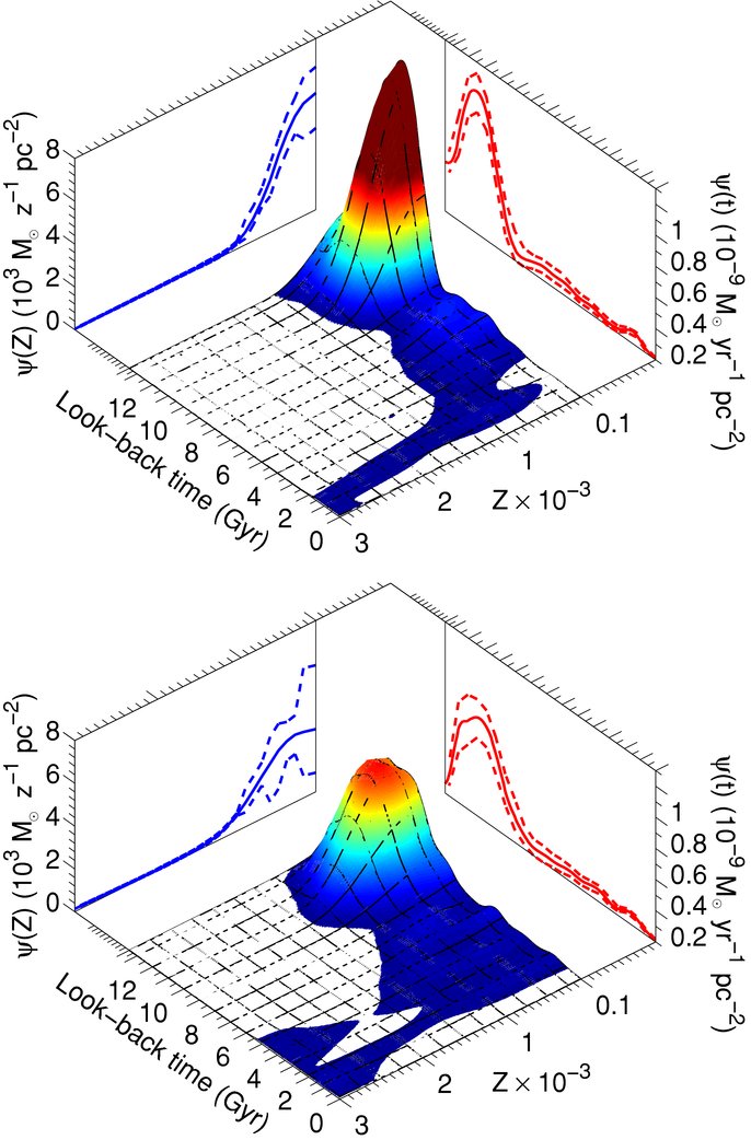
Figure 14. Statistical significance of the SFH of LGS-3. Solid lines show the SFH of LGS-3 and its error interval. Thick dashed line shows the average of the SFHs of five subsets of stars of LGS-3 each one containing 50% of the stars randomly selected. The results of the tests were normalized by scaling by a factor of two. Thin dashed lines show the rms deviations of the five solutions.
Download figure:
Standard image High-resolution image
Footnotes
- *
Based on observations made with the NASA/ESA Hubble Space Telescope, obtained at the Space Telescope Science Institute, which is operated by the Association of Universities for Research in Astronomy, Inc., under NASA contract NAS 5-26555. These observations are associated with program 10505.
- 13
Local Cosmology from Isolated Dwarfs: http://www.iac.es/project/LCID/