


ABSTRACT
Magnetic field data acquired by the Ulysses spacecraft in high-speed streams over the poles of the Sun are used to investigate the normalized magnetic helicity spectrum σm as a function of the angle θ between the local mean magnetic field and the flow direction of the solar wind. This spectrum provides important information about the constituent modes at the transition to kinetic scales that occurs near the spectral break separating the inertial range from the dissipation range. The energetically dominant signal at scales near the thermal proton gyroradius k⊥ρi ∼ 1 often covers a wide band of propagation angles centered about the perpendicular direction, θ ≃ 90° ± 30°. This signal is consistent with a spectrum of obliquely propagating kinetic Alfvén waves with k⊥ ≫ k∥ in which there is more energy in waves propagating away from the Sun and along the direction of the local mean magnetic field than toward the Sun. Moreover, this signal is principally responsible for the reduced magnetic helicity spectrum measured using Fourier transform techniques. The observations also reveal a subdominant population of nearly parallel propagating electromagnetic waves near the proton inertial scale k∥c/ωpi ∼ 1 that often exhibit high magnetic helicity |σm| ≃ 1. These waves are believed to be caused by proton pressure anisotropy instabilities that regulate distribution functions in the collisionless solar wind. Because of the existence of a drift of alpha particles with respect to the protons, the proton temperature anisotropy instability that operates when Tp⊥/Tp∥ > 1 preferentially generates outward propagating ion-cyclotron waves and the fire-hose instability that operates when Tp⊥/Tp∥ < 1 preferentially generates inward propagating whistler waves. These kinetic processes provide a natural explanation for the magnetic field observations.
Export citation and abstract BibTeX RIS
1. INTRODUCTION
This paper presents an analysis of solar wind magnetic field fluctuations measured by the Ulysses spacecraft. Our emphasis here is on the normalized magnetic helicity σm, which is the magnetic helicity spectrum divided by the magnetic energy spectrum, a quantity that takes values in the interval −1 < σm < 1. A closely related quantity, the reduced magnetic helicity spectrum, can be measured in the solar wind by virtue of Taylor's hypothesis and a technique developed by Matthaeus et al. (1982) and Matthaeus & Goldstein (1982). Solar wind measurements at 1 AU show that in the inertial range the quantity σm fluctuates randomly between +1 and −1 indicating that the magnetic helicity in the inertial range is approximately zero, on average (Matthaeus & Goldstein 1982; Goldstein et al. 1994; Smith 2003). However, in the so-called dissipation range, the σm spectrum is different. Measurements of σm in the dissipation range usually show a nonzero magnetic helicity signature that can be caused by waves with a right-hand sense of polarization propagating predominantly outward, away from the Sun (Goldstein et al. 1994; Leamon et al. 1998b, 1998a; Smith 2003; Hamilton et al. 2008).
At first, this was thought to be a consequence of collisionless damping of a cascade of nearly parallel propagating left-hand polarized ion-cyclotron waves (ICWs) at the proton inertial length k∥c/ωpi ∼ 1. A simultaneous cascade of nearly parallel propagating right-hand polarized whistler waves are not damped at that scale and may thus produce the observed signal (Goldstein et al. 1994). But, if solar wind turbulence is composed primarily of a cascade of highly oblique Alfvén waves as incompressible MHD turbulence simulations and theories suggest (Shebalin et al. 1983; Oughton et al. 1994; Goldreich & Sridhar 1995; Matthaeus et al. 1996; Boldyrev 2006; Schekochihin et al. 2007, 2009), then the explanation for the σm spectrum may be different than first thought. At kinetic scales k⊥ρi ∼ 1, where ρi is the thermal proton gyroradius, the oblique Alfvén wave with k⊥ ≫ k∥ becomes the kinetic Alfvén wave (KAW) and the polarization of the KAW becomes right-handed as first discovered by Gary (1986). Thus, a spectrum of oblique KAWs propagating predominantly outward, away from the Sun, will also produce a right-handed magnetic helicity signature that is consistent with solar wind data as first pointed out by Howes & Quataert (2010).
To further investigate the origin of the magnetic helicity signature observed in the dissipation range of solar wind turbulence, the purpose of the present study is to analyze the normalized magnetic helicity spectrum as a function of the angle θ between the flow direction and the direction of the local mean magnetic field  . This analysis allows one to associate angles of propagation with different spectral features and to tentatively identify the waves responsible for the right-hand polarization signature seen by previous investigators using traditional Fourier spectral analysis. The technique used here was first introduced by He et al. (2011) and applied to study high-speed solar wind streams in the ecliptic plane near 1 AU. In the present study, the same technique is used to analyze high-speed streams outside of the ecliptic plane—over the poles of the Sun—using data from the Ulysses spacecraft.
The results reported here partially support the hypothesis that the right-hand polarized σm signature observed at k⊥ρi ∼ 1 using traditional Fourier analysis techniques is primarily caused by a nearly perpendicular propagating spectrum of KAW waves, in agreement with the scenario proposed by Howes & Quataert (2010). But there is at least one result of the data analysis that raises serious doubts about this physical interpretation as is explained in the conclusions. The results also show the existence of a nearly parallel propagating component of the wave spectrum localized around k∥c/ωpi ∼ 1, a component first seen in the angular decomposition of the σm spectrum performed by He et al. (2011). The existence of these parallel propagating waves had previously been inferred from the enhancement in magnetic field fluctuations near parallel propagation at k∥c/ωpi ∼ 1 observed by Podesta (2009) and Wicks et al. (2010) using a novel solar wind analysis technique introduced by Horbury et al. (2008) and reviewed by Podesta (2010). They may be closely related to the enhancements in solar wind density fluctuations at the proton Larmor radius scale reported by Neugebauer (1975, 1976). The parallel propagating electromagnetic waves in question are likely the copious waves first observed by Behannon (1976) and recently rediscovered by Jian et al. (2009, 2010).
Behannon (1976), in a comprehensive study of interplanetary magnetic field (IMF) data from 0.46 to 1 AU, identified many examples of coherent, nearly parallel propagating, transverse electromagnetic waves having both right- and left-hand polarization and frequencies between 10−2 and 10 Hz in the spacecraft frame. Many more examples have been investigated by Jian et al. (2009, 2010). Based on the general knowledge of solar wind distribution functions and the related plasma instabilities at the time, Behannon (1976) concluded that the waves "may be associated with temperature anisotropy-driven instabilities" (see, for example, Hollweg 1975; Gary et al. 1976). A similar explanation was put forward by Neugebauer et al. (1978) for the enhancements in density fluctuations observed by Neugebauer (1975, 1976). In the present study, it will be shown that the magnetic helicity observations of parallel propagating waves reported here also point to pressure- or temperature-driven instabilities as the most likely generation mechanism. Remarkably, the powerful data analysis technique employed in this study is providing valuable new insights that shed light on the nature and composition of solar wind fluctuations at kinetic scales and the kinetic processes that operate there.
The contents of this paper may be summarized as follows. Section 2 discusses the data used in this study. Section 3 describes the details of the data analysis techniques. The results of the data analysis and a discussion of the physical interpretation of these results are presented in Section 4. A summary of the results and the conclusions of this study are contained in Section 5.
2. DATA SELECTION AND CHARACTERIZATION
The data analyzed in this study consist of data from the vector helium magnetometer on board the Ulysses spacecraft (Balogh et al. 1992), data acquired during the first southern polar pass in late 1993 and 1994 and the first northern polar pass in 1995 (Smith & Marsden 1995; Marsden & Smith 1997; Balogh et al. 2001). These two phases of the mission occurred near the solar minimum in 1996 and under typical solar minimum conditions so that all the time intervals studied here pertain to high-speed flows with average radial speeds usually greater than 700 or 750 km s−1. The heliocentric distance of the spacecraft (radial distance) decreased monotonically from approximately 4 AU to 1.8 AU during the first southern polar pass, 1993 November through 1994 November, and then increased monotonically from approximately 1.5 AU to 3 AU during the first northern polar pass, 1995 May through December; see Figure 1. These are the time periods analyzed here. Related studies of the same time periods have been performed by many investigators including Balogh et al. (1995), Goldstein et al. (1995), Horbury et al. (1995a, 1995b, 1996), and Forsyth et al. (1996).
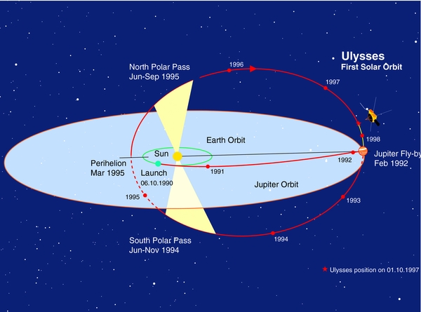
Figure 1. Schematic diagram of Ulysses first orbit.
Download figure:
Standard image High-resolution imageHigh time resolution 1 s magnetic field data and lower resolution ∼8 minute plasma data employed in this study are publicly available through the NASA CDAWeb Internet site http://cdaweb.gsfc.nasa.gov/. Although the magnetic field data have a nominal 1 s cadence (sampling time), the time cadence of the data sometimes changes to 1/2 s or 2 s and, in addition, data gaps of various durations occur somewhat randomly throughout the data set. In this study, time intervals were selected for analysis based on a strict selection criterion such that no data gaps larger than 3.8 s are allowed. This ensures adequate coverage of small scales and, in particular, the kinetic scales k⊥ρi ∼ 1 and k∥di ∼ 1 that constitute the main focus of this study. Most of the data selected for analysis contain no data gaps greater than 2 s and in each time interval the total number of gaps ⩾2 s represents a negligible fraction of the total duration of the time interval. As part of the selection process, the data for each of the magnetic field components were visually inspected for outliers and unusual behavior. Once a time interval was selected for analysis, the data were linearly interpolated onto a time grid having a uniform cadence of precisely 1 s, thereby smoothly interpolating any data gaps and any data with a 1/2 s cadence.
The durations of the time intervals analyzed in this study range in size from approximately 8 hr to 16 hr or more. Most of the intervals have a duration between 8 and 11 hr. The existence of gaps in the spacecraft data limited the duration of the selected time intervals to less than 16 hr, roughly. Intervals meeting the selection criteria but lasting for less than approximately 8 hr were not used. Longer time intervals are preferable since they usually provide better angle coverage at the timescales of primary interest, approximately 1–10 s. Nevertheless, many of the intervals provide little or no coverage in the important range of angles nearly parallel to the local mean magnetic field. Intervals that sample the full range of angles from the parallel direction through the perpendicular direction are, of course, of special interest. In all, a total of 182 distinct time intervals were analyzed in this study. Of those, 90 provide coverage spanning the full range of angles.
The characteristic plasma parameters for each solar wind interval were obtained using plasma data from the SWOOPS instrument (Bame et al. 1992). Average values of the proton number density np, proton temperature Tp, and magnetic field strength B0 taken over each time interval were used to compute estimates of the proton thermal gyroradius ρi = vth, i/Ωi and proton beta βp = npkBTp/(B20/2μ0), where  is the proton thermal speed, Ωi = eB0/mp is the proton cyclotron frequency, kB is Boltzmann's constant, μ0 is the permeability of free space, e > 0 is the proton charge, and mp is the proton mass. The proton temperature was crudely estimated as the average of the two radial proton temperatures Tlarge and Tsmall provided in the data set. Taylor's hypothesis τ = λ/VR is used to estimate the timescale τ in the spacecraft frame that corresponds to the wavelength λ in the plasma frame. If VR is the average radial solar wind speed over a given time interval, then the wavenumber where k⊥ρi = 1 is approximately equivalent to the timescale τ = 2πρi/VR. This timescale is marked on the spectral measurements for reference. The ratio of the wavenumbers k⊥/k∥ such that k⊥ρi = 1 and k∥di = 1, where di = c/ωpi is the proton inertial length, is k⊥/k∥ = β1/2i. The ratio of the corresponding timescales in the spacecraft frame, using Taylor's hypothesis, is τ∥/τ⊥ = β1/2i. For the Ulysses data analyzed here, the proton temperatures are on the order of 10 eV and typical values of βi range from 1 to 2.5.
3. ANALYSIS PROCEDURE
Each time interval is analyzed using a two-step procedure. In step 1, the magnetic energy spectrum (trace spectrum), the magnetic helicity spectrum, and the normalized magnetic helicity spectrum σm are computed using traditional Fourier transform techniques. In step 2, the magnetic helicity spectrum and magnetic energy spectrum are both computed as a function of the angle θ between the local mean magnetic field and the average flow direction using wavelet techniques. The results from steps 1 and 2 are then compared to see what signals in the angular σm spectrum are responsible for producing the σm signal observed in the Fourier spectrum and to determine the possible wave modes which these signals represent. The details of the analysis procedures are described in the following two subsections.
3.1. Fourier Spectral Analysis
Fourier spectra are computed for each of the three RTN components of the magnetic field vector using standard fast Fourier transform (FFT) techniques as described in Chapter 6 of Percival & Walden (1993). The trace spectrum or total magnetic energy spectrum EB is equal to the sum of the spectra for the three orthogonal components BR, BT, and BN. Because of the large dynamic range of solar wind spectra, the spectral analysis is performed using a data taper (data window) which consists of a discrete prolate spheroidal sequence with a time-bandwidth product NW = 4 (Percival & Walden 1993). The procedure used to compute the spectra is briefly summarized as follows; further details can be found in Percival & Walden (1993). First, the mean value is subtracted from the time series, then the time series is multiplied by the data taper (window function), the length of the resulting time series is doubled by zero padding, and then the FFT is applied to obtain the raw spectrum given by the square amplitudes of the Fourier coefficients. The raw spectrum is smoothed by means of convolution with a Papoulis window function. The bandwidth Δf of the smoothing window is frequency dependent such that Δf/f = 7% and the smoothed spectrum is evaluated on a uniformly spaced frequency grid in log–log space.
The reduced magnetic helicity spectrum is obtained from the relation
where k1 is the wavenumber in the radial direction, Im(z) is the imaginary part of the complex number z, and Sr23(k1) is the reduced cross-spectrum between BT and BN. This important result, first derived by Matthaeus & Goldstein (1982), allows the reduced magnetic helicity spectrum in the solar wind to be measured using data from a single spacecraft provided Taylor's hypothesis holds. The normalized magnetic helicity spectrum is given by
which takes values in the interval −1 < σm < 1. The procedure used to compute σm is briefly summarized as follows. First, the mean value is subtracted from each of the time series BT(t) and BN(t). Both time series are then multiplied by the data taper (window function) and the length of the resulting time series are both doubled by zero padding. The FFT is applied to each time series and the raw cross-spectrum Sr23 is evaluated as the product of the Fourier coefficients of BT times the complex conjugates of the Fourier coefficients of BN. This raw cross-spectrum is smoothed by means of convolution with a Papoulis window function with a frequency-dependent bandwidth such that Δf/f = 7% and the smoothed spectrum is evaluated on a uniform frequency grid in log–log space that coincides with the grid used to compute the spectrum EB. The normalized magnetic helicity σm is then evaluated using the formula
obtained from Equations (1) and (2), where f is the frequency in the spacecraft frame.
3.2. Wavelet Analysis
The wavelet analysis procedure is similar to that employed in the study by Podesta (2009) and is based on the Morlet wavelet

where ω0 = 6. The analysis covers the range of timescales from s = 2 s to s = 100 s using a uniformly spaced grid in log–log space with a total of 50 grid points. At any given time tn, the local mean magnetic field at a given scale s is equal to
where the normalization factor is given by
For time series data, the local mean magnetic field is defined by
where
The results of the spectral analysis of the time series data are binned according to the angle θ between the local mean magnetic field  and the heliocentric radial direction
  as described below. The direction
  is approximately equal to the average flow direction of the solar wind since VR ≫ |VT| and VR ≫ |VN|. The angle is given explicitly by

Thus, θ may take any value in the range 0° ⩽ θ ⩽ 180°. Previous studies by Horbury et al. (2008) and Podesta (2009) have found that the power in the magnetic field fluctuations is azimuthally symmetric about the direction of the local mean magnetic field so measurements of the azimuthal dependence have not been attempted here.
The energy or power in the magnetic field component BR at time t and at the scale s is proportional to  , where
  is the wavelet coefficient
tn = nΔt, and "*" denotes the complex conjugate (Podesta 2009, Equation (13)). The quantity of primary interest is the normalized magnetic helicity σm. By analogy with Equation (3), the normalized magnetic helicity at a given time t and scale s is defined by
where  ,
,  , and
, and  are the wavelet coefficients of the signals BR(t), BT(t), and BN(t), respectively. This is the same formula employed by He et al. (2011). The wavelet coefficients are computed using the procedure described by Podesta (2009).
The average power at a given scale s is

where the brackets denote a time average (an average over tn, n = 1, 2, ..., N) and a constant coefficient that is independent of scale has been omitted for simplicity. The average power when the local mean magnetic field lies in the angular interval θa < θ < θb is equal to
where the average includes only those times tn for which θa < θn < θb and θn is the direction of the local mean magnetic field at time tn and scale s given by Equation (9). Similarly, the average normalized magnetic helicity when the local mean magnetic field lies in the interval θa < θ < θb is defined by
This quantity has the important property that −1 < σm(s, θ) < 1 and is the same definition adopted by He et al. (2011). The average power (13) and the normalized cross helicity (14) are both computed as a function of the angle θ for each time interval of solar wind data analyzed here. The angle bins used in this study have a width of 6°. The endpoints of the angle bins are 0°, 6°, 12°, 18°, ..., 180°.
4. RESULTS
The results from the first northern polar pass of Ulysses are shown in Figure 2 and the results from the first southern polar pass are shown in Figure 3. Note that the results have been plotted as a function of the timescale of the fluctuations in the spacecraft frame, although from a physical point of view it is more useful to plot them versus k⊥ρi using Taylor's hypothesis. The timescale corresponding to k⊥ρi ≃ 1 has been marked by a dashed line in the figures for reference. Only spectra that cover the complete range of parallel and perpendicular directions are included in the figure sets given in Figures 2 and 3; this requirement selected 90 out of the 182 spectra analyzed in this study. It should be noted that a small percentage of these spectra have marginally adequate (perhaps inadequate) statistics in the bin closest to the parallel direction or in the vicinity of data dropouts (white patches) and this may cause false σm signals in some instances, especially near θ = 0° or θ = 180° and more often at scales greater than 10 s. It should be kept in mind that the data processing is not flawless.

Figure 2.
Example of the reduced magnetic helicity spectrum σm (upper left), trace magnetic power spectrum (lower left), magnetic helicity spectrum as a function of angle θ between  and the flow direction (upper right), and the trace magnetic power spectrum as a function of angle (lower right) observed during the first northern polar pass. The physical units of the power spectrum in the lower right are arbitrary. The dashed line indicates the approximate scale where kρi = 1. The proton beta for this interval is βp ≃ 1.7. (The complete figure set (30 images) is available in the online journal.)
Download figure:
Standard image High-resolution image
Figure 3.
Example of the reduced magnetic helicity spectrum σm (upper left), trace magnetic power spectrum (lower left), magnetic helicity spectrum as a function of angle (upper right), and the trace magnetic power spectrum as a function of angle (lower right) observed during the first southern polar pass. The physical units of the power spectrum in the lower right are arbitrary. The dashed line indicates the approximate scale where kρi = 1. The proton beta for this interval is βp ≃ 1.4. (The complete figure set (62 images) is available in the online journal.)
Download figure:
Standard image High-resolution imageFrom 1993 through 1995, the radial component of the large-scale solar magnetic field was directed radially outward over the northern hemisphere (positive polarity) and radially inward over the southern hemisphere (negative polarity). As a consequence, the magnetic helicity spectra obtained during the northern polar pass, Figure 2, and the southern polar pass, Figure 3, usually exhibit opposite polarities (opposite algebraic signs). The same change in polarity is observed for σm spectra observed in different magnetic sectors in the ecliptic plane (Goldstein et al. 1994; Leamon et al. 1998b; He et al. 2011).
At the proton Larmor radius scale k⊥ρi ≃ 1, indicated by the dashed line in the upper right-hand panel in Figure 2, the yellow patch in the neighborhood of θ = 90° is tentatively identified as the KAW signal as explained below. The lower right-hand panel in Figure 2 shows that at kinetic scales (timescales in the neighborhood of the dashed line) the perpendicular power is larger than the parallel power implying that most of the power at those scales is concentrated in the vicinity of the yellow patch. Note that the algebraic sign of the yellow patch in the upper right-hand panel matches the sign of the σm signal in the upper left-hand panel, σm > 0, as it should if the yellow patch is the dominant cause of that signal.
The magnetic helicity spectrum is logically divided into two parts, parallel propagating fluctuations and perpendicular or obliquely propagating fluctuations. The parallel propagating fluctuations appear as a colored patch on the magnetic helicity spectrum usually within 10° or 20° of the parallel direction (θ = 0° or θ = 180°); for example, the blue patch in the upper right-hand panel of Figure 2. The perpendicular propagating fluctuations appear as a colored patch around 90° ± 30°, such as the yellow patch in the upper right-hand panel in Figure 2, although oblique signals with smaller and larger angular ranges are also observed. The subsections below describe the observations and physical interpretations for these two classes of fluctuations. It must be emphasized that all the signals appearing in the magnetic helicity spectrum are believed to be electromagnetic perturbations or waves since, if they were electrostatic perturbations ( ), then they would not generate a magnetic field signature. In this discussion, the terms "signals" and "contiguous colored patches" are synonymous.
4.1. Parallel Propagating Fluctuations
The dark blue patch close to the parallel direction θ = 0 in the upper right-hand panel in Figure 2 and similar parallel signals found in other intervals are most naturally explained as being caused by electromagnetic ICWs propagating away from the Sun nearly parallel to the local mean magnetic field or by whistler waves propagating toward the Sun nearly parallel to the local mean magnetic field. These waves are believed to be caused by proton pressure anisotropy instabilities and related distribution function anisotropies which are ubiquitous in the solar wind plasma (Gary et al. 2001, 2002; Kasper et al. 2002; Marsch et al. 2006). In a majority of those intervals where there is good spectral coverage in the parallel direction, the parallel power is seen to rise slightly at scales where a strong parallel signal occurs, such as the dark blue patch in Figure 2. Consequently, this spectral feature is not believed to be part of the turbulent energy cascade which, according to the model of incompressible MHD turbulence, is expected to exhibit monotonically decreasing power as the scale size decreases in the parallel direction. We believe that this parallel power is injected at scales k∥c/ωpi ∼ 1 by plasma instabilities as previously surmised by several investigators (Behannon 1976; Neugebauer et al. 1978; Podesta 2009; Wicks et al. 2010, and others).
The parallel propagating ICW is a left-hand polarized electromagnetic wave such that, for propagation that is radially outward (away from the Sun), σm < 0 if  and σm > 0 if
  (here
(here  is the local mean magnetic field), in agreement with the majority of observations for parallel propagation in Figures 2 and 3. In a stable plasma the ICW is strongly Landau-damped at k∥c/ωpi ∼ 1, but when Tp⊥ ≫ Tp∥ the plasma is unstable to the generation of parallel propagating ICWs at k∥c/ωpi ∼ 1. Moreover, when there is a field-aligned drift velocity
  between the alpha particles and the protons, as is often observed in the solar wind at 1 AU, then the maximum growth rate of the instability is larger in the direction of
  (Gary et al. 2003; Podesta & Gary 2011). The latter feature is necessary to explain the observations presented in this study since ICWs propagating with equal powers both parallel and anti-parallel to
  would produce a vanishing magnetic helicity signature σm = 0, which is not observed. In the solar wind,
  is usually directed away from the Sun and approximately parallel to
  (Marsch et al. 1982; Kasper et al. 2008).
The parallel propagating whistler mode is a right-hand polarized electromagnetic wave such that, for propagation radially inward (toward the Sun), σm > 0 if  and σm < 0 if
  , consistent with many of the observations in Figures 2 and 3. When Tp∥ ≫ Tp⊥, the plasma is unstable to the generation of parallel propagating whistler waves at k∥c/ωpi ∼ 1. This is a type of fire-hose instability. Moreover, when there is a field-aligned drift between the alpha particles and the protons, then the maximum growth rate for this instability is larger in the direction anti-parallel to
  (Podesta & Gary 2011). Thus, the dark blue patch in Figure 2 is consistent with outward propagating ICWs generated by the electromagnetic ion-cyclotron instability when Tp⊥ > Tp∥ or by sunward propagating whistler waves generated by the fire-hose instability when Tp∥ > Tp⊥. In this mechanism, the direction of propagation of ICWs is always outward, in the direction of the alpha–proton drift velocity, and the direction of propagation of the whistlers is always inward, opposite to the direction of the alpha–proton drift velocity, independent of the IMF polarity (Podesta & Gary 2011). Which wave is driven unstable depends on the sign of the proton pressure anisotropy. The regulation of plasma pressure anisotropies through this mechanism has been discussed by Kennel & Scarf (1968), Eviatar & Schulz (1970), Hollweg (1975), Schwartz (1980), Gary et al. (2001), and by many others, although the effects of the alpha–proton drift on these instabilities have not been studied in detail until recently (Podesta & Gary 2011).
In the spacecraft frame, the timescale at which these instabilities are observed is equivalent, by Taylor's hypothesis, to the spatial scale k∥c/ωpi ∼ 1 and is equal to β1/2i times the timescale marked by the dashed line in the figure, where βi is the proton beta. The physical interpretation just described can be further confirmed by finding the times of occurrence of the most intense parallel waves in the data, such as those that produce the blue patch in Figure 2, and by comparing these with the observed temperature anisotropies of the ions at those same times. However, this would also require a definitive identification of the wave modes and their propagation directions which is not possible without low-frequency electric field data. Another possibility is to see if the parallel waves consistently disappear during intervals with very small temperature anisotropies. This has not been attempted here.
4.2. Perpendicular Propagating Fluctuations
The perpendicular fluctuations usually show a signature indicative of a right-hand sense of polarization for outward propagating waves, such as the yellow patch in the upper right panel in Figure 2. At small scales, the power is usually greater for near-perpendicular angles than for near-parallel angles as seen, for example, in the lower right-hand panel in Figure 2. Although, it should be noted that in a few of the observations the parallel signal at k∥c/ωpi ∼ 1 is so intense that it has roughly the same power as the perpendicular power at the same scale. More often, however, the perpendicular signal dominates the power at kinetic scales (k⊥ρi ∼ 1) which partly explains why at these scales the magnetic helicity spectrum obtained using Fourier transform techniques, the upper left panel in Figure 2, has approximately the same magnitude and the same algebraic sign as that for the perpendicular fluctuations in the upper right panel in Figure 2. But, even if the parallel signal has equal power, the perpendicular signal will still dominate the total power because the fraction of time the magnetic field points in the near-parallel direction is almost always small compared to the fraction of time it points in the oblique directions (Podesta 2009) and, consequently, the oblique and/or perpendicular σm signal will dominate the time average affected by the Fourier transform.
The perpendicular propagating fluctuations observed in the solar wind near k⊥ρi ∼ 1 are believed to consist mainly of KAWs propagating away from the Sun with k⊥ ≫ k∥ and with  of predominantly one sign. This conclusion is based on previous work which demonstrates that in the wavenumber range k⊥ρi ∼ 1 solar wind fluctuations are predominantly composed of KAWs with k⊥ ≫ k∥ (Leamon et al. 1999; Bale et al. 2005; Howes et al. 2008; Sahraoui et al. 2010); although, for a different point of view see Narita et al. (2011). In particular, Bale et al. (2005) have shown that the measured phase velocity of Alfvénic fluctuations is consistent with the dispersion relation for KAWs and with a transition from highly oblique Alfvén waves at MHD scales to KAWs at k⊥ρi ∼ 1. Howes et al. (2008) have shown using gyrokinetic simulations of Alfvénic turbulence spanning the range from MHD scales to kinetic scales that energy spectra for electric and magnetic fields are in qualitative agreement with the in situ observations presented by Bale et al. (2005). More direct observational evidence for the existence and dominance of KAWs come from measurements by Sahraoui et al. (2010) of the frequency and wavevector spectrum of the waves in the plasma frame using the three-dimensional wave telescope technique. These novel measurements show that at k⊥ρi ∼ 1 the wavevectors of the waves have wave normal angles near 85° with respect to
  and that the dispersion relation in the plasma frame is in reasonable agreement with that for KAWs. Hence, it is reasonable to conclude that the perpendicular signal observed in the magnetic helicity versus angle spectra in the present study is predominantly caused by KAWs.
Gary (1986) has shown that for KAWs with k⊥ ≫ k∥, the magnetic helicity approaches zero at MHD scales and takes values of order unity at kinetic scales, k⊥ρi ≳ 1, such that
indicating a right-hand sense of polarization of the wave (with respect to the direction of  ). This appears to explain why the perpendicular σm signals observed in the solar wind remain near zero at MHD scales and then "turn on" at kinetic scales, although a zero σm signal could also be caused by a wavevector spectrum that is an even function of
  . Howes & Quataert (2010) have shown that a spectrum of KAWs in which
  is of predominantly one sign, say
  , will give rise to a normalized magnetic helicity spectrum σm that is consistent with solar wind observations at 1 AU. However, if instead the KAW spectrum is an even function of k∥, then the σm spectrum observed by a single spacecraft vanishes. This further supports the view that in the neighborhood of k⊥ρi ∼ 1, solar wind fluctuations consist of KAWs propagating away from the Sun with k⊥ ≫ k∥ and with
  of predominantly one sign. It should be noted, however, that the peak values of the σm spectra observed using Ulysses data, |σm| ≃ 0.25, are much smaller than the near unity values expected if
  is of one sign only (see, for example, Figure 2 in Howes & Quataert 2010). This implies that there must be a non-negligible component of sunward propagating KAWs that causes a reduction in the observed value of σm or, possibly, that there may be some other waves or physical processes involved which are not yet understood. The former possibility is consistent with the idea that the fluctuations are turbulent, meaning that nonlinear interactions at these kinetic scales are not negligible, an idea supported by observations of power-law spectra extending from proton kinetic scales to much smaller electron scales (Sahraoui et al. 2009; Kiyani et al. 2009; Alexandrova et al. 2009).
In general, from Equation (15), it follows that when the large-scale solar magnetic field  is directed radially outward, as it is during Ulysses' northern polar pass, a perpendicular signal with a positive magnetic helicity signature σm > 0 is consistent with a spectrum of oblique KAWs which are predominantly propagating away from the Sun and such that
  . Likewise, when the large-scale IMF
  is directed radially inward, as it is during Ulysses' southern polar pass, a perpendicular signal with a negative magnetic helicity signature σm < 0 is consistent with a spectrum of oblique KAWs which are predominantly propagating away from the Sun and such that
  .
.
5. DISCUSSION AND CONCLUSIONS
A study of the normalized magnetic helicity spectrum as a function of the angle θ between the solar wind flow direction and the direction of the local mean magnetic field  has been carried out using Ulysses data characteristic of sustained high-speed solar wind streams over the poles of the Sun around solar minimum. By focusing on the important range of kinetic scales k⊥ρi ∼ 1 and k∥c/ωpi ∼ 1, the results presented here shed new light on the kinetic plasma processes that operate at these scales. While the observations at MHD scales are consistent with a vanishing magnetic helicity spectrum as previous measurements have shown, the observations at kinetic scales show at least two distinct populations of fluctuations, one that occurs at angles nearly parallel to
  and another that occurs at oblique angles centered approximately perpendicular to
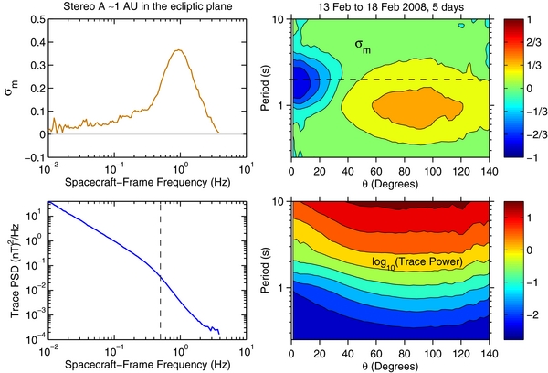
  . Two distinct populations are also found for high-speed streams in the ecliptic plane (He et al. 2011), as the example in Figure 4 shows, and have likewise been observed using new multi-spacecraft analysis techniques (see the upper panel in Figure 3 in Narita et al. 2011). Note that the contours in Figure 4 are much smoother than those in Figures 2 and 3 because the spectra in Figure 4 are based on the analysis of a five-day interval whereas the spectra in Figures 2 and 3 are each based on approximately 8–12 hr of data. Hence, the spectra in Figure 4 represent a time average over a much longer time interval and this yields better statistics.
Figure 4. Analysis of a five-day interval of high-speed wind observed in the ecliptic plane near 1 AU by the STEREO A spacecraft. This is one of the same intervals studied by Podesta (2009). The dashed line indicates the approximate scale where kρi ≃ 1 and for the plasma parameters here βp ≃ 2. The data were analyzed using the same procedure used to obtain the spectra in Figures 2 and 3 except that the angle bin width was 2 5 instead of 6°. Note that one-day subintervals of this five-day interval have been analyzed by He et al. (2011).
Download figure:
Standard image High-resolution image
The physical characteristics of the parallel and perpendicular wave populations at high heliographic latitudes are found to be qualitatively and quantitatively similar to those in the ecliptic plane. These characteristics may be summarized as follows. In many of the intervals presented in Figures 2 and 3, a large magnetic helicity signature |σm| ≃ 1 was found near k∥c/ωpi ∼ 1, usually within 10° or 20° of the direction parallel to  . These signals are not believed to be caused by the turbulence which primarily transfers energy toward perpendicular wavevectors, even at kinetic scales. We believe that the observed parallel signals are caused by left-hand polarized ICWs propagating outward, away from the Sun, or by right-hand polarized whistler mode waves propagating inward, toward the Sun. This interpretation is consistent with the regulation of solar wind pressure anisotropies through plasma instabilities since in the presence of an outward drift of alpha particles with respect to the protons—a drift along the direction parallel to
  —the proton temperature anisotropy with Tp⊥ > Tp∥ favors the growth of outward propagating ICWs and the fire-hose instability with Tp∥ > Tp⊥ favors the growth of inward propagating whistlers, independent of the direction of
  or of the dominant polarity of the IMF (Podesta & Gary 2011). This is a logical physical interpretation for the measured signals near the parallel direction.
The perpendicular propagating fluctuations typically form a wide angular band, θ ≃ 90° ± 30°, and are the energetically dominant fluctuations at MHD scales but, at kinetic scales, intense parallel waves can occasionally have power similar in magnitude to that of the perpendicular fluctuations. The magnetic helicity signature of the perpendicular fluctuations is approximately zero at MHD scales and usually shows a predominance of right-hand polarization with a typical amplitude |σm| ≃ 0.25 at kinetic scales for the Ulysses data studied here. The signal around 90° in the σm versus θ spectra matches the magnetic helicity signature seen in the Fourier transform spectra at these scales, both in sign and amplitude, as a consequence of the fact that solar wind time series usually contain relatively few periods when the IMF is nearly parallel to the flow (see, for example, Figure 4 in Podesta 2009). The perpendicular fluctuations are most naturally associated with Alfvénic fluctuations at MHD scales and with KAW fluctuations at kinetic scales, consistent with previously obtained evidence (Leamon et al. 1999; Bale et al. 2005; Howes et al. 2008; Sahraoui et al. 2010). However, the existence of a nonvanishing σm signal for KAWs requires that the waves propagate predominantly outward so that  is predominantly of one sign. Otherwise, if the energy spectrum were an even function of
  , then the perpendicular σm signal would necessarily vanish. In summary, the observations are consistent with a dominant population of outward propagating KAWs (
 of one sign) accompanied by a subdominant population of inward propagating KAWs (
 of opposite sign) that may all be nonlinearly interacting.
One aspect of the measurements presented here that is puzzling is the wide angular extent of the supposed KAW signal. Solar wind measurements by Sahraoui et al. (2010) using the wave telescope technique show that around k⊥ρi ∼ 1, the wavevectors in the KAW spectrum are concentrated between 80° and 90°, implying an angular width of approximately 10° and this seems consistent with what is expected for a critically balanced cascade. However, the majority of measurements presented in Figures 2 and 3 in the present study often exhibit angular widths in excess of ±20°. It is not known why the angular widths obtained using these two different measurement techniques are quantitatively different. However, it should be kept in mind that the two quantities being measured are very different: the wavevector  on the one hand and the magnetic helicity σm on the other hand.
A more serious issue concerns the observed balance or imbalance of energies of inward and outward propagating fluctuations. At kinetic scales, the data in Figure 4 clearly indicate that in the neighborhood of θ = 90° where k⊥ ≫ k∥ the power is an even function of k∥. That is, for the population of perpendicular waves there is equal power for propagation toward or away from the Sun. By symmetry, this implies that the "KAW" signal in the σm versus θ spectrum must vanish. If so, then it may be that the σm signal observed near 90° is instead caused by plasma instabilities, such as the oblique mirror instability and the oblique fire-hose instability, rather than by the KAW cascade. This may also explain the wide angular extent of the signal and, consequently, this possibility needs further investigation. The oblique mirror and oblique fire-hose instabilities are also believed to play a role in the regulation of pressure anisotropies in the solar wind (see, for example, Bale et al. 2009 and references therein).
Another puzzle is why the measurements in Figure 4 show that the power is symmetric about θ = 90° in the range 50° ≲ θ ≲ 140° (lower right panel), while the measurements shown in Figure 4 of Sahraoui et al. (2010) show that for the random sample of measured wavevectors there are many more wavevectors propagating outward,  , than inward,
  . Even though the measurements presented in Figure 4 above reflect a much larger statistical sample than the data presented by Sahraoui et al. (2010), this appears to be a serious discrepancy that needs further investigation.
The knowledgeable reader may wonder how the data in the lower right panel in Figure 4, which indicate that for k⊥ ≫ k∥ the KAW spectrum is an even function of k∥, can be reconciled with the established notion that Alfvénic fluctuations in the solar wind are predominantly outward propagating. There is no contradiction here. The fact is that for strong incompressible MHD turbulence it is possible for the two Elsasser spectra to have different amplitudes while, at the same time, they are both azimuthally symmetric and even functions of k∥. In fact, numerical simulations of incompressible MHD turbulence necessarily satisfy the property ![$\bm w^+(-\bm k,t) = [\bm w^+(\bm k,t)]^*$](https://content.cld.iop.org/journals/0004-637X/734/1/15/revision1/apj389068ieqn49.gif) and
and ![$\bm w^-(-\bm k,t) = [\bm w^-(\bm k,t)]^*$](https://content.cld.iop.org/journals/0004-637X/734/1/15/revision1/apj389068ieqn50.gif) , where
, where  are the Elsasser fields,
  is the wavevector, and "*" denotes the complex conjugate. This is required for the fields to be real valued. Hence, if solar wind turbulence is axisymmetric about the direction of the local mean magnetic field as is clearly evident in the inertial range analyses of Horbury et al. (2008) and Podesta (2009), then the three-dimensional turbulence spectra must be even functions of k∥, even when the cross helicity is very different from zero. Thus, the data in Figure 4 showing that in the neighborhood of θ = 90° the spectrum is an even function of k∥ are entirely consistent with the hypothesis that solar wind turbulence is strong, meaning that large numbers of Fourier modes are simultaneously excited and nonlinearly interacting.
Useful discussions with Joe Borovsky, Ruth Skoug, Chuck Smith, Melvyn Goldstein, and Fouad Sahraoui are gratefully acknowledged. This work was supported by the NASA Solar and Heliospheric Physics Program and the NSF SHINE Program.