


ABSTRACT
We have extended the recent analyses of magnetohydrodynamic third moments as they relate to the turbulent energy cascade in the solar wind to consider the effects of large-scale shear flows. Moments from a large set of Advanced Composition Explorer data have been taken, and chosen data intervals are characterized by the rate of change in the solar wind speed. Mean dissipation rates are obtained in accordance with the predictions of homogeneous shear-driven turbulence. Agreement with predictions is best made for rarefaction intervals where the solar wind speed is decreasing with time. For decreasing speed intervals, we find that the dissipation rates increase with increasing shear magnitude and that the shear-induced fluctuation anisotropy is consistent with a relatively small amount.
Export citation and abstract BibTeX RIS
1. INTRODUCTION
The layers above the Sun's photosphere receive heating that overcomes the gravitational potential and thus causes its atmosphere to accelerate and develop an outgoing flow. Regions of slow and fast wind emanate from the Sun, ranging in speed at 1 AU from about 300 to 800 km s−1. These winds interact with each other as they travel outward. The evolving velocity shears in the wind are an important driver of the interplanetary turbulence and impact in detail the properties of the turbulent fluctuations (Coleman 1968; Roberts et al. 1992; Matthaeus et al. 1996b; Roberts & Ghosh 1999; Goldstein et al. 1999, 2003; Breech et al. 2009).
The direct measurement of the nonlinear turbulent energy cascade rate comes from evaluating third moments of the magnetohydrodynamic (MHD) variables in the relation of Politano & Pouquet (1998a, 1998b), where the third moments are proportional to the scale times the dissipation rate. This work has been carried out at 1 AU using Advanced Composition Explorer (ACE) data (MacBride et al. 2005, 2008; Stawarz et al. 2009, 2010) and in polar winds near 3 AU using Ulysses data (Sorriso-Valvo et al. 2007; Forman et al. 2010). In all the above work, no analyses distinguishing the velocity shear were made.
Recently, Wan et al. (2009, 2010a, 2010b) have derived modified third-moment equations for incompressible MHD with homogeneous shear. This new theory introduces two new terms to the Politano and Pouquet equations. These new terms are proportional to the shear times certain integrals over the second moment which are sensitive to anisotropy in the second moment. This approach can be used to approximate the influence of shear away from boundaries and for regions where the speed varies nearly linearly with position. We have adapted these ideas to single-spacecraft analysis techniques and present the first observational results from the application of this approach to the solar wind at 1 AU.
In Section 2, we discuss the basic theory and determine the necessary relations to be used for the observational analyses presented in Section 3. Section 4 discusses the results, and Section 5 summarizes the conclusions.
2. THEORETICAL APPROACH AND APPLICATION TO SOLAR WIND DATA
We want to examine the role of large-scale velocity shear in generating and modifying the MHD turbulence in the solar wind near 1 AU. At large scales, kinetic energy significantly exceeds magnetic energy, and thus the energy-containing scale of interplanetary turbulence is dominated by the contribution of velocity shear. This velocity shear is a source of the turbulent energy cascade. In addition, the velocity shear affects the flux of the energy through the inertial range and imposes a peculiar anisotropy on the fluctuations in addition to what arises from the presence of the magnetic field.
The role of velocity shear in turbulence is more profitably examined first with respect to hydrodynamics (HD) in Section 2.1 and then applied to MHD in Section 2.2. From the HD case, we will see that the anisotropy in the second moment contributes with the shear to the evaluation of the energy dissipation rate.
2.1. Third Moments and Hydrodynamics
The Navier–Stokes equations for incompressible HD and constant density can be re-expressed under assumptions of homogeneous fluctuations to yield a relation between the mean rate of energy dissipation per unit mass  and correlation functions of velocity v. This approach is used to describe turbulent fluctuations with a large number of degrees of freedom such that the fluctuations become well behaved in a statistical sense. In these situations, velocity shears associated with turbulent eddies are presumed to exist over a large range of directions and to vary in speed up and down with equal repetition so that the average shear is zero. More explicitly, v is a random variable whose average is centered at zero and has the same statistical properties everywhere so as to satisfy homogeneity. The energy cascade is forward from larger to smaller scales, and this corresponds to a positive value of .
von Kármán & Howarth (1938) re-expressed the Navier– Stokes equations in the above manner for homogeneous isotropic turbulence. Their resulting equation and its generalizations will be referred to as the KH equation. Kolmogorov (1941a, 1941b) introduced increments of velocity δv(≡ v(x + r) − v(x), where r is the spatial separation lag). Like differential quantities in the Navier–Stokes equations, these increments are sensitive to the flow dynamics and for the given flow are also homogeneous. Kolmogorov recast the KH equation in terms of δv, and in doing so, he derived the four-fifths law of isotropic and fully developed HD turbulence in the limit of small but inertial range r. His findings state that 〈(δvr)3〉 = −(4/5)r, where δvr are increments of the longitudinal velocity (i.e., components of velocity along the lag direction r) and 〈⋅⋅⋅〉 is the ensemble average of the enclosed quantity. Here, the third power of the increment, called a third-order structure function, varies linearly with lag r, has the opposite sign to r, and is proportional to the . Monin (1959; see also Monin & Yaglom 1975) showed that (in the inertial range where viscous terms may be neglected) the KH equation is generalizable to anisotropic turbulence as ∇ · 〈(δv)2δv〉 = −4, where (δv)2 ≡ δv · δv. This vector form may be simplified to one dimension by integrating it over the volume of the sphere of radius r, and applying Gauss' theorem to the divergence operator to get a surface integral. In this paper, we use the KH in spherical average form
where dΩ(≡ sin θdθdϕ) is the element of solid angle, θ and ϕ are spherical polar coordinates, and  is the unit radial vector normal to the sphere (see Nie & Tanveer 1999). The integral in Equation (1) is carried out over all angles and normalized by 4π, and so calculates the scale-to-scale flux of energy through the sphere. In Equation (1) and throughout the remainder of the paper, we assume statistically stationary flow. Owing to this, also equals the energy cascade rate. Equation (1) is valid regardless of the anisotropy of the δv. Note that the integral of the third-order structure function is negative, linear in radius (r is always nonnegative in spherical coordinates), and proportional to . The sense in which v is a homogeneous field is critical to the derivation of the KH equation. Here, v refers to a fluctuating velocity with a mean value that is zero everywhere.
Casciola et al. (2003) obtained a different third-moment equation for examining the role of velocity shear on turbulence in the absence of boundary effects. They set

Equation (2) separates total velocity into a fluctuation component u and a varying mean part U. Here the mean velocity is incompressible and is restricted to a plane-parallel shear flow that varies linearly with position. This case is referred to as a homogeneous shear flow (e.g., Hinze 1975; Townsend 1976; Davidson 2004). As such, increments of U for any lag are the same no matter the position of the origin. Casciola et al. call v in Equation (2) a homogeneous field, but we do not since the average of v varies with position. As such, the velocity used in the KH equation given by Equation (1) will not prove to be interchangeable with the one given by Equation (2). The decomposition of velocities into fluctuating and mean parts also follows the Reynolds analysis of the Navier–Stokes equations and usefully employs results from this approach. The Navier–Stokes equation is then rewritten in a similar manner as the KH equation. The resulting equation will have structure functions that are separated into parts showing the role of the background shear. Numerous experiments have explored quasi-homogeneous shear flows. These include physical experiments (e.g., Champagne et al. 1970; Harris et al. 1977; Shen & Warhaft 2000, 2002) and numerical simulations (e.g., Rogers & Moin 1987; Lee et al. 1990; Kida & Tanaka 1994; Pumir & Shraiman 1995; Pumir 1996; Schumacher & Eckhardt 2000; Schumacher 2004; Gualtieri et al. 2002; Casciola et al. 2003, 2007).
For the homogeneous velocity shear and without loss of generality, we select a coordinate system so that the background flow magnitude varies linearly with position in a single direction across the flow. Taking the background velocity U to be  , its gradient is
  , where α is the magnitude of speed change with position and is a constant because the solution of the mean momentum equation has U independent of time. The mean kinetic energy is then fixed as its production and dissipation are balanced by its convection in the mean gradient direction (e.g., Champagne et al. 1970). Fluctuations on the background shear have velocities u in all three directions and vary with position in all three directions. Casciola et al. (2003) derive an equation for this case in terms of velocity increments and averaged over of a sphere of radius r. The resulting equation is referred to here as the Casciola–Gualtieri–Benzi–Piva (CGBP) equation. We neglect a viscous term for r values greater than the dissipative scales, and in terms of structure functions, the CGBP equation is given by
where
and
Here, the superscript HD refers to the hydrodynamic case, δu(≡ u(x + r) − u(x)) is the increment of u along the lag, and (δu)2 ≡ δu · δu. Integrals are definite. In Equations (4) and (5), they are evaluated over all angles, and in Equation (6) they are evaluated over the spherical volume with radius r. SHD3 is the third moment due to fluctuations alone and has the same form as the left-hand side of Equation (1). The terms SHDU and SHDP are proportional to the shear, and their values are reliant on the particulars of the fluctuation anisotropy in the (trace and off-diagonal x–y element of the tensor) second moment in the presence of shear. The term SHDU calculates the flux of energy through the sphere due to shear, while SHDP is the shear production of energy in the volume.
From Equation (3), the sum of the individual terms on the left-hand side is linear with r. Casciola et al. (2003) used three-dimensional (3D) incompressible HD numerical simulations to examine a linearly varying plane shear flow with turbulent fluctuations (see also Gualtieri et al. 2002). From the simulation results, they found that the fluctuations satisfy Equation (3) well in the inertial and energy-containing ranges. The individual terms themselves are not, however, linear with r. The sum of transfer terms SHD3 and SHDU is most significant in the inertial range, corresponding to the cascade of energy from larger to smaller scales. In the energy-containing scales, both of these transfer terms become small at large r. The term SHDP can be insignificant at the smallest scales of the inertial range but becomes significant in the energy-containing range, and the dominant term at large r. It is referred to as the shear production term because it accounts for the energization of the cascade. The sum SHD3 + SHDU is comparable to SHDP at the scale rs = (/|α|3)1/2 (Toschi et al. 1999).
The importance of the terms is certainly affected by the magnitude of α. In the limit α = 0, Equation (3) reduces to the KH equation given by Equation (1). In the opposite limit of large |α|, we can consider |α|r ≫ [δu(r)]rms, where [δu(r)]rms is the root-mean-squared value of δu averaged over all angles at fixed r. For this condition, |SHD3| can be small compared to either |SHDU| or |SHDP| or to both. If only one term proportional to α remains in this limit in Equation (3), then the corresponding fluctuation correlation is independent of r. This situation is likely in the energy-containing range where |SHDU| ≪ |SHDP| when r ≫ rs. It might also occur within a large inertial range if |SHDU| ≫ |SHDP| and [δu(r)]rms/|α| ≪ r ≪ rs.
The SHD3 term can contribute significantly to the cascade even when the fluctuations are isotropic or nearly so. For smaller r, fluctuations tend to become more isotropic (e.g., Hinze 1975) due in part to the effects of pressure strains that cancel relative to energy scale transfer, but not for energizing fluctuation velocity components of the same scale. As a result, SHD3 is likely to be dominant at the small-scale end of the inertial range, and isotropy can be used to estimate this term.
The shear term SHDU is sensitive to the fluctuation anisotropy and so is more difficult to estimate. In Equation (5), the angular sensitivity comes from the projection of δU onto the normal to the sphere  . The factor sin θcos ϕ is from the projection along the flow direction
  onto
onto  , and the sin θsin ϕ part is from the projection along the flow gradient direction
  onto
onto  . With this projection, an isotropic fluctuation energy dependence, or one where the fluctuation energy is isotropic in the x–y plane, causes SHDU to vanish. This velocity shear in 3D is, however, associated with the nonlinear vortex stretching of eddies. It is known to yield a strain along two principal axes in the x–y plane located half-way between
  and
and  (see Tennekes & Lumley 1972; Kundu 1990). Along one axis, the vorticity and energy of eddies are maximally amplified at the expense of these same quantities along the other axis. The principal axis on which eddies are amplified or not reverses with the sign of α. This contributes to fluctuation anisotropy and gives SHDU a negative value.
The strain associated with vortex stretching also causes the correlation between δux and δuy to become nonzero. This is a condition indicative of anisotropic fluctuations. For α > 0, this correlation is negative, and for α < 0 this correlation is positive. As a result, SHDP will have a negative value. Lumley (1967) used dimensional analysis to determine the value of the 〈uxuy〉 omni-directional spectrum in the inertial range of a homogeneous shear flow turbulence. He showed that the Kolmogorov energy cascade would be associated with a k−7/3 wavenumber spectrum for 〈uxuy〉. This indicates that the corresponding second-order structure function 〈δuxδuy〉 should vary as r4/3.
To evaluate cases for a homogeneous velocity shear, we need to use the CGBP equation and not the KH equation. To illustrate this, we replace δv in Equation (1) with δu + δU as would occur when the velocity shear is not detrended. We then obtain
where SHDextra is given by
and the cubic term involving δU vanishes upon integration. These extra terms do not equate with SHDP in Equation (3), and thus the value of obtained from Equation (7) would differ from that in Equation (3).
When solar wind velocity shear intervals of particular magnitude and sign are combined, the background velocity is not spatially invariant. This situation requires using the generalization of the CGBP equation to MHD. Moreover, we will need a method for representing the shear-induced anisotropy to evaluate a term analogous to SHDU, which will rely heavily on the above discussed vortex stretching process. We now turn to consider the above approach to MHD.
2.2. Third Moments and Magnetohydrodynamics
The incompressible (single fluid) MHD equations that are normally written in terms of the Elsässer variables Z±(=V ± B/(4πρ)1/2, where V is the velocity, B is the magnetic field, and ρ is a constant density) can also be re-expressed using the same assumptions for HD as relations between and third-order structure functions. In this paper, the magnetic Prandtl number is assumed to be unity so that viscosity and resistivity are made equal. The two-dimensional (2D) and 3D cases without shear were derived by Politano & Pouquet (1998a, 1998b), and we will refer to these relations as the PP equations. For this paper, the 3D PP equations in spherical average form are given by
where δZ± ≡ Z±(x + r) − Z±(x) and (δZ±)2 ≡ δZ± · δZ±. The integral represents the flux of the energy from scale to scale through the sphere. Equation (9) is quite general and valid for both anisotropic turbulence and for flow with zero average shear.
The total rate T is given by T = (+ + −)/2 and is also the mean dissipation rate. The (twice) total fluctuation energy per unit mass is given by the sum ((δZ+)2 + (δZ−)2)/2 which is why the sum of rates leads to the rate for total energy. The difference corresponds to the cross-helicity σc which is normalized by total energy and is given by ((δZ+)2 − (δZ−)2)/((δZ+)2 + (δZ−)2).
Wan et al. (2009, 2010a, 2010b) examined the resulting relations for MHD when the velocity is separated into fluctuations and background linear shear flow in both two and three dimensions. Wan et al. (2010b) particularly focus on the 2D case where the velocity and magnetic field fluctuations are confined to a plane, and where there is no background magnetic field. In this 2D case, the fluid vorticity is nonlinearly strained via electrodynamic vortex amplification associated with a differential Lorentz force (e.g., Spangler 1999). They undertook incompressible 2D MHD numerical simulations with periodic boundaries of driven turbulence amidst a velocity shear. The prescribed time constant background velocity varied up and down spanwise, and sharply between two regions of nearly linear shear. In the linear shear region, the contributions from fluctuations and shear terms were evaluated and found to be in good agreement with theory. They showed that the power spectrum of the fluctuations exhibits anisotropic behaviors at lower wavenumbers. This is induced by the velocity shear which, judging from their Figure 10, is oriented approximately with principal axes that are streamwise and spanwise. Power is greater in the spanwise direction. Moreover, they considered the total velocity without any detrending for shear, and the 2D PP equations were found to give good estimate of the cascade rate when the entire spatial domain was considered so that the net shear vanished.
In the solar wind, the effects of the velocity shear influence fluctuations with vectors and variations in all three spatial directions. Moreover, there is a background interplanetary magnetic field B0 that must also be considered, and here we assume that B0 is a constant. We set

where z± = u ± b/(4πρ)1/2 is the fluctuating part, b is the fluctuating magnetic field, and the mean velocity is as in Section 2.1. Wan et al. (2009) derive the shear expressions from the 3D MHD equations that we refer to here as the Wan–Servidio–Oughton–Matthaeus (WSOM) equations. The WSOM equations are obtained using the fluctuating and mean parts and integrating over a spherical volume. We recast the equations in a form analogous to Equation (3) as
where

and
Again we have neglected dissipative terms since the application will be for lags longer than the dissipation scale. The nature of the terms and limits with respect to α are in accord with the above discussion for HD. Summing over the ± terms in Equations (11)–(14) and then dividing by 2 gives the corresponding dissipation rate for total energy. The WSOM equations are valid for any form of anisotropic turbulence which arises in association with the velocity shear.
When σc = 0, all corresponding ± terms in Equations (12)–(14) are equal to each other (SMHD, +3 = SMHD, −3, etc.) and contribute to the forward energy cascade so that each term is nonpositive. When σc = ±1, nonlinearity in the incompressible MHD equations vanishes and so should all terms. For intermediate σc, there is no known constraint on the sign of the terms. The expectation is that for σc not near ±1, the cascade will be forward and all terms in Equations (12)–(14) will be nonpositive.
Equation (11) provides what is needed to examine simulation results from incompressible 3D MHD quasi-homogeneous shear flow. Yet, the solar wind is a flow where the ratio of the plasma to magnetic pressure is typically below unity, and thus is far from an incompressible medium. Here, B0 and its attendant anisotropy with respect to direction become vitally important. Turbulent velocity and magnetic field fluctuations in the presence of B0 nonlinearly interact most strongly across B0 (e.g., Shebalin et al. 1983; Matthaeus et al. 1996a). With highly oblique wave vectors, the fluctuations are found to approach a nearly incompressible (e.g., Zank & Matthaeus 1993) or weakly compressive (e.g., Bhattacharjee et al. 1998) state. For this case, the incompressible MHD equations contain the dominant nonlinear effects needed to describe the turbulent fluctuations. Observations show that interplanetary fluctuations are relatively noncompressive in the inertial range. Moreover, lags across B0 are readily available at 1 AU. MacBride et al. (2005, 2008) showed from Equation (9) with B0-directed anisotropy models that the cross-field cascade in the solar wind is indeed stronger than along B0. The amount of anisotropy is modest enough that an isotropic approximation for Equation (9) is still useful in cascade rate determination (see also Stawarz et al. 2010). We will henceforth ignore anisotropy arising from B0 in order to focus on velocity shear.
In order to proceed further with solar wind data analyses, we need to consider approximations for the individual terms in Equation (11) since single-spacecraft analyses lack direct measurement of fluctuation anisotropy with respect to the velocity shear. Again, because we are going to combine intervals with a particular varying background velocity, we must use the WSOM equations to obtain and not the PP equations, for the same reasons discussed earlier concerning the HD case. In Section 3, we show that the PP equations, using only the observed lag measurements and assuming isotropy to evaluate the integral in Equation (9), yield incorrect results for such cases.
In Equation (11), the terms SMHD, ±U require anisotropy, and thus we treat first the estimation of these terms. The SMHD, ±U terms from Equation (13) involve an integral over the fluctuation energy that vanishes for isotropic fluctuations in the x–y plane. With the assumed form of the velocity shear and with fluctuations varying in all three spatial dimensions, the most straightforward expectation for fluctuation energy anisotropy induced by the shear is the alignment of this anisotropy with the mean strain principal axes  . This is due to the aforementioned mechanism of vortex stretching. We can evaluate the integral in Equation (13) by assuming that the fluctuation energy [δz±(r, ϕ, θ)]2 varies with θ and ϕ in the simplest possible manner: θ and ϕ vary according to an ellipsoidal model with coefficients that are independent of r so that the anisotropy is constant with r. This neglects the expected attenuation of anisotropy for smaller r in the inertial range. In the solar wind, however, the inertial range is moderately short, and moreover the estimates for will be based on averages taken over the observed linear range of r. Thereby, the model coefficients can approximate an average anisotropy over the extent of this range. In this approach, the range of coefficients is limited to values where mean dissipation and expected plasma heating rates are in acceptable agreement.
We replace [δz±(r, ϕ, θ)]2 with f(ϕ, θ)[δz±(r)]2 where
is the ellipsoid of anisotropy with principal axes radii a and b in the x–y plane and the out of plane axis with radius c. (Note that a larger radius along its axis corresponds to smaller amplitude along that axis for fixed radius r.) The value of f is normalized so that 4π results when f is integrated over all solid angle. The mean values 〈[δz±(r)]2〉 over all angles can be related to the values along the streamwise lag 〈[δz±(r, 0, 90°)]2〉. The values along the streamwise lag are hereafter denoted by 〈[δz±(r)]2s〉, that in application will be replaced by measured values from solar wind data. Dividing through with the value of f in the x direction, we obtain

where the factor As ≡ 1/f(0, 90°) is given by
or more compactly by
With these assumptions, the resulting form for Equation (13) is
which is independent of c by virtue of the cancellation of factors in Equations (15) and (17). We assume that the forward energy cascade is enhanced by both SMHD, +U and SMHD, −U when they are nonzero because the data used in Section 3 combine intervals without regard for σc. The average |σc| is not so large as to significantly alter the inertial range cascade (Smith et al. 2009; Stawarz et al. 2009). With this assumption, we take absolute values in Equation (19) so that SMHD, ±U is always nonpositive. This then means that we can also take b2 ⩾ a2 without loss of generality and not be concerned with the sign of α when evaluating Equation (19). Note that isotropy in the x–y plane a2 = b2 gives SMHD, ±U = 0. Moreover, the choice of principal axes in the x–y plane in Equation (15) maximizes |SMHD, ±U| for fixed x–y anisotropy b2/a2, whereas if the axes were along  and
and  , SMHD, ±U are zero. Alternatively, for fixed values of SMHD, ±U, b2/a2 is minimized because a different orientation for the principal axes in the x–y plane requires larger b2/a2 to obtain the same values of SMHD, ±U.
The model Equation (19) will be essential in the analyses below. The values of a and b are to be taken as free parameters to vary anisotropy in the x–y plane and to examine the resulting values of ± to compare with independently determined dissipation and heating rates. We neglect the effect of σc in the present analysis and use the same parameters a, b, and c for the Elsässer amplitudes |z+| and |z−|. Taking a case from Section 3, one sets a = 1, and b = 2, then SMHD, ±U = −0.08|α|r〈(δz±)2〉 with a proportionality constant of 0.08. The actual range of the proportionality constant is quite limited. The largest magnitude is 2/15 and occurs when b2/a2 → ∞. As a result, the magnitudes of SMHD, ±U are sensitive to small departures from isotropy but insensitive to large departures.
Remaining terms on the left-hand side of Equation (11) give nonzero values even for isotropic fluctuations, but the underlying fluctuations will be anisotropic for finite α. To lowest order, we expect the anisotropy of these terms to align with the mean strain principal axes. We approximate the anisotropy as one equivalent to the fluctuation energy and separate integrands as quantities whose angular dependence is given by Equation (15) and whose amplitude dependence is only on r. The integration over all angles of f(ϕ, θ) only results in the cancellation of the 4π factor in Equations (12) and (14). The mean value of the amplitude dependence ratioed to that measured in the streamwise direction is proportional to As. This introduces a dependence upon the free parameter c, as well as a and b. From Equation (12), the terms dependent only on fluctuations are estimated by

which retain the signs of the third-order structure functions along the streamwise lag. The shear production terms SMHD, ±P involve an evaluation over the volume. With this approach, we use the streamwise values of 〈δz±xδz∓y〉 so that
With increasing r, the values of SMHD, ±P accumulate and generally increase in magnitude. Note that absolute values are not introduced in Equation (21) because the signs and magnitudes of the integrands are obtained with measurements. Their relation with the sign of α will give a consistency check on the assumption that velocity shear driving of turbulence is preeminent.
The dependence of As on c can vary the magnitude of the estimates for SMHD, ±3 and SMHD, ±P. For the typical case in Section 3, a = c = 1 and b = 2, we find from Equation (18) that As = 1.2 which differs little from complete isotropy where a = b = c = 1 and As = 1. In the limit that c2/a2 → ∞, which corresponds to fluctuation wave vectors confined increasingly to the x–y plane, As = 2/3. In the opposite limit where c2/a2 → 0 and b2/a2 is finite, As → ∞, so that large anisotropy in the z direction can greatly affect the values of SMHD, ±3 and SMHD, ±P.
The final expressions used in the present analyses change some notation and this notation is consistent with that used in MacBride et al. (2005, 2008) and Stawarz et al. (2009, 2010). The signs of Z± and z± are redefined with respect to the background magnetic field so as to correspond to propagating Alfvén waves traveling inward to (denoted by superscript "I") or outward from (denoted by "O") the Sun. (Note that propagation here can be a formality since in directions where k · B0 = 0, Alfvén waves do not propagate and yet eddies with mixed Elsässer signs do interact nonlinearly.) The background velocity is mainly in the heliocentric radial direction  away from the Sun. In Cartesian coordinates, this corresponds to the
  direction used above. We take
  to be in the direction of the Earth's revolution about the Sun which is the
  direction of the Radial–Tangential–Normal (RTN) coordinate system. The RTN coordinate system is used in the present analyses of ACE spacecraft measurements. The measured lag is taken from VSWτ, where VSW is the solar wind speed and τ is the time lag of increments. Since the wind carries the fluctuations past the spacecraft, the increasing time lag corresponds to positions going back to the Sun, so that the spherical radius lag r is replaced by the Cartesian lag −VSWτ. We hereafter also drop the subscript denoting streamwise measurements, and the superscript MHD since that is the only case we will consider. Equation (11) with all approximations included is rewritten as
where the functions of VSWτ are

and
We also define the sum of structure functions in Equation (22) by

and total structure functions by


and

The total and mean dissipation rate is given by

The subscript "SH" denotes that the expressions correspond to the WSOM theory for the case of homogeneous shear, and use detrended velocities to evaluate fluctuations and their moments. Note that the sign of the structure functions as most naturally sampled with the spacecraft is positive when the energy cascade is forward.
For comparison purposes, the case with total velocity given by Equation (9) without detrending and ignoring shear uses

assuming isotropy. (Note that the DU and DP terms are not relevant here since total velocity is used.) The total rate ignoring shear is taken from

and

Here the subscript "NOSH" denotes no shear.
We now turn to ACE observations.
3. DATA ANALYSES
We use a merged 64 s data set from the ACE spacecraft's thermal proton instrument SWEPAM and magnetic field instrument MAG. These data are taken at 1 AU and span 10 years from 1998 until the end of 2007. A wide range of solar wind conditions are encompassed in these data including solar minimum and solar maximum conditions, as well as intervals of increasing and decreasing solar wind speed associated with velocity shears.
The analyses of MacBride et al. (2005, 2008) and Stawarz et al. (2010) have demonstrated that the PP equations given by Equation (9) can provide scale-independent mean dissipation rates within the inertial range at 1 AU. Since stationary conditions are assumed, the mean dissipation rate is equivalent to the cascade rate of the turbulent energy. The calculated rates match up well with inferred proton heating rates in the solar wind. In this study we use the WSOM equations and the modified third-moment shear expressions DI/O3, SH(VSWτ) described in Section 2 to analyze solar wind observations with regard to velocity shear.
Plasma and magnetic field measurements are combined into individual intervals with period lengths satisfying lower and upper bounds. A lower bound is set by the correlation of time of the turbulent fluctuations (∼1 hr), and an upper bound by the need to select intervals where the VSW follows a linear trend. We have considered two interval times tinterv of 6 and 12 hr which meet the above bounding criteria. Additionally, we remove intervals containing coronal mass ejections and other transients based on a list of known events, and intervals with fewer than 50% of the total possible proton number density measurements. This latter criterion excludes intervals that most often have VSW < 300 km s−1 where plasma measurements are relatively less accurate.
We compute values of both TSH and TNOSH based on the 6 and 12 hr intervals. The method for computing TNOSH is the same as that used by MacBride et al. (2005, 2008) and Stawarz et al. (2009, 2010), while the method used to compute TSH is a slightly modified version of the same procedure.
Computed moments from intervals with 12 hr are found to give results consistent with those from 6 hr. Thereby, we present only the results for 12 hr which is also the same interval size used by Stawarz et al. (2009, 2010) to display their results.
The shear analyses assume a uniform shear, and hence we need to obtain the linear trend in each data interval. We perform a linear fit of the radial velocity data in each 12 hr interval and subtract the linear trend from the raw radial velocity data set. This gives us the linear trend characterizing the shear and a detrended set of data characterizing velocity fluctuations.
In the solar wind, we take the directions R (radially outward from the Sun) and T (in the direction of the Sun's rotation) to correspond to the x and y directions in the theory. In other words, we are assuming the gradient to be in the (R, T) plane. This neglects any latitudinal component to the shear and is the natural starting point for a single-spacecraft analysis. We will return to this assumption in Section 4. The background solar wind velocity is mainly in the R direction, but varies with time at the spacecraft and has a gradient in the T direction due to the rotation with the Sun of sources of different solar wind speeds. Then, the wind speed is constant on the local Parker spiral, so that α = ∂VSW/∂T is given by

where ΔVSW is the change in speed based on the linear trend for the whole 12 hr interval and is in units of km s−1, R = 1 AU is heliocentric distance, Ω = (2π/27) day−1 is the synodic angular frequency of solar rotation taken to be the value near the solar equator, and tinterv = 0.5 days is used. Note that ΩRtinterv corresponds to a distance traversed along a circular arc for time tinterv owing to solar rotation.
Fluctuation velocity and magnetic field data, and the proton density, which is averaged for the 12 hr interval, are used to compute (δzI/O)2δzO/IR, (δzI/O)2 and δzI/ORδzO/IT as a function of time lag for each 12 hr interval. These quantities are then interpolated to a grid of spatial lag based on the average VSW for the interval. This grid has a range and points that are common to all 12 hr intervals analyzed and is used to construct ensemble averages discussed further below. The above fluctuation moments along with α and the chosen free parameters a, b, and c are then used to calculate DI/O3, DI/OU, DI/OP, and DI/O3, SH as a function of the spatial lag given by Equations (23)–(26), as well as the total quantities DT3, DTU, DTP, and DT3, SH given by Equations (27)–(30).
When using the PP equations, we compute (δZI/O)2δZO/IR as a function of time lag for each 12 hr interval, which is equivalent to DI/O3, NOSH given by Equation (32). Values are interpolated onto a common spatial grid based on the average VSW for the 12 hr interval. The same interpolation is made for values of DT3, NOSH given by Equation (34).
In addition, the expected proton heating rate heat for each 12 hr interval is calculated and when ensemble averaged is compared to a mean dissipation rate. The proton heating rate is inferred from the radial gradient of the R-component of proton temperature and for 1 AU is given by

where VSW is the average solar wind speed within the 12 hr interval in units of km s−1 and TP is the average R-component of proton temperature in units of Kelvin (Vasquez et al. 2007).
Averaging the 12 hr interval quantities, we carry out two analyses. First, in Section 3.1, we subset intervals into bins of velocity shear and examine the predictions of the WSOM equations and those of shear-driven turbulence. Second, in Section 3.2, we bin according to VSWTP and reanalyze the results by Stawarz et al. (2010) using the WSOM equations. This compares the WSOM approach to the PP approach in a setting where both are applicable.
3.1. Sorting Results by Local Velocity Shear
In order to apply Equations (22)–(31), intervals are sorted into bins according to ΔVSW in a specified range. The ΔVSW bins that we use range from −100 to +100 km s−1 with equal widths of 25 km s−1. Note that negative values of ΔVSW correspond to regions where faster wind is followed by slower wind so that these are regions of rarefaction. Positive values of ΔVSW correspond to regions where a slower wind is being overtaken by a faster wind, and thus these are regions of compression.
The present analysis bins compression and rarefaction intervals for equivalent levels of shear without regard for the duration of the event. With equivalent levels of shear, the theory has dissipation rates that are the same in the rarefaction and compression intervals. Important differences in these intervals when analyzed, however, will be shown below. This might arise due to assumptions in our analysis such as the neglect of latitudinal gradients. Our theory, in general, is symmetric regardless of whether the shear is positive or negative. Results are shown without additional comment on these assumptions. Section 4 then discusses how the assumptions can impact the results.
Averages over the 12 hr intervals having ΔVSW within the appropriate bins are performed to find the average value of DT3, SH as a function of spatial lag. Then the uncertainty-weighted average of 3DT3, SH/(4 r) is calculated for each spatial lag r which is less than the corresponding time lag τ of 8000 s based on a reference speed of 400 km s−1. The long-lag limit is further constrained so that DT3, SH varies almost linearly from the shortest lag to the long-lag limit. The linear scaling of DT3, SH is required by the theory. This constraint is further shown below to be important when ΔVSW > 0. This calculation gives the average TSH for each bin. A similar approach is used to obtain TNOSH.
To compute uncertainties we use the same method described in Stawarz et al. (2009, 2010). Take X to be some quantity, e.g., DI/O3, at a particular spatial lag, which is to be averaged over the 12 hr intervals analyzed. Each value of X computed from an individual 12 hr interval is taken to be a statistically independent estimate with no intrinsic uncertainty because 12 hr is greater than the correlation length and the propagation of measurement error is likely the same for all samples. As such, estimates from the 12 hr intervals will follow a Gaussian distribution, and Gaussian statistics can be used to compute the mean standard deviation and error of the mean for the ensemble-averaged quantities. From there this uncertainty can be propagated through further calculations using standard methods.
The average value of heat is also obtained from all 12 hr intervals per ΔVSW bin. The expression for heat in Equation (37) is determined by an analysis based on the spherically symmetric proton equation of state. Hence, the heating rate is the average over the spherical polar angles and so does not correspond to rates in separate rarefaction and compression regions. Based on the work of Burlaga & Ogilvie (1973) who found that the net heating in compressions over rarefaction is ∼15% on average, we would expect that the ΔVSW > 0 bins have somewhat more heating than predicted by heat, while ΔVSW < 0 bins would have less. The amount of relative deviation is, however, likely to be only ≲ 5%. Thus, heat is deemed to be a sufficiently good guide to the required dissipation rate from the turbulence in the present analyses. Uncertainty for the average value of heat is determined as above.
Figure 1 plots the value of TSH, TNOSH, and heat as a function of ΔVSW (see also Table 1). Here the value of TSH is obtained by assuming an anisotropy of 2:1, corresponding to the values a = c = 1 and b = 2 in Equations (18) and (24). Errors of the mean are plotted but are typically smaller than the symbols used, and horizontal bars indicate the range of ΔVSW analyzed for each data point. Except for TNOSH, the plotted rates increase with |ΔVSW|, as would be expected of a turbulent energy cascade driven by velocity shear. The values of TSH and heat approximately follow each other, and TSH is always above zero, consistent with a forward cascade dissipating and heating the plasma. The dissipation rate TNOSH ignoring shear appears to be dominated by the sign of the shear and has no correspondence with heat. The absolute value of TNOSH is smaller for the bin with ΔVSW < 0 than the one for the same but positive signed ΔVSW bin.

Figure 1. Mean dissipation rate vs. ΔVSW for 12 hr intervals and comparison with the average proton heating rate. The no-shear analysis is dominated by the signal from the background shear. The shear analysis yields acceptable results for ΔVSW < −25 km s−1. Error bars are smaller than symbols. Table 1 gives plotted data values, errors, and sample numbers.
Download figure:
Standard image High-resolution imageTable 1. Rates for Figure 1
| ΔVSW Range | Number of | TSH |
TNOSH |
Theat |
|---|---|---|---|---|
| (km s−1) | Samples | (× 103 J kg−1 s−1) | ||
| −100 < ΔVSW < −75 | 159 | 3.94 ± 0.11 | −4.59 ± 0.09 | 2.39 ± 0.14 |
| −75 < ΔVSW < −50 | 404 | 3.20 ± 0.05 | −2.75 ± 0.04 | 1.94 ± 0.07 |
| −50 < ΔVSW < −25 | 915 | 1.56 ± 0.03 | −1.89 ± 0.03 | 1.63 ± 0.05 |
| −25 < ΔVSW < 0 | 1334 | 0.62 ± 0.06 | −0.85 ± 0.02 | 1.54 ± 0.04 |
| 0 < ΔVSW < +25 | 782 | 0.32 ± 0.11 | 1.41 ± 0.04 | 1.72 ± 0.05 |
| +25 < ΔVSW < +50 | 410 | 1.51 ± 0.29 | 5.18 ± 0.09 | 2.36 ± 0.09 |
| +50 < ΔVSW < +75 | 204 | 1.18 ± 0.34 | 9.66 ± 0.12 | 2.70 ± 0.13 |
| +75 < ΔVSW < +100 | 136 | 6.59 ± 0.38 | 16.94 ± 0.26 | 3.02 ± 0.17 |
Download table as: ASCIITypeset image
The values of TSH for the bins closest to zero, i.e., −25 to 0 km s−1 and 0 to +25 km s−1, in Figure 1 are anomalously small compared to heat and are not a good match. The poor match probably occurs because cases of weak shear are less likely to be characterized well by a linear trend of velocity shear. In these cases, the intervals tend to be located between intervals of positive and negative shear and may be at local maximum or minimum VSW. Thus, we will focus on the outlying bins where the shear is more significant and better characterized.
The farther outlying bins on the left and negative side of ΔVSW = −25 km s−1 have TSH that matches or exceeds heat. These can then provide sufficient energization for the plasma including electron and alpha heating, as well as proton heating. Taking electron heating to be about 50% of proton heating provides a good upper bound to the expected total plasma heating (Vasquez et al. 2007; Stawarz et al. 2010), and the values obtained for TSH can satisfy these bounds. On the other hand, farther outlying bins on the right and positive side of ΔVSW = +25 km s−1 have a more irregular up and down trend with respect to heat and are less in agreement with heat than is the case on the opposite side. This is not a trend to be expected for an ensemble of true homogeneous shear-driven turbulence, where the sign of α or ΔVSW does not affect the mean dissipation rate. Section 4 discusses how compressional regions in the solar wind can deviate from the theory and contribute to the observed trends.
The analysis based on the PP equations giving TNOSH clearly does not provide the mean dissipation rate for cases with persistent shear. This was explained in Section 2, and these results are in agreement with conclusions reached there. The signal from the velocity shear itself contaminates the measurements to such an extent that the sign of the calculated TNOSH is the same as that of ΔVSW.
We now consider the relative contribution of fluctuation-only and shear-dependent terms to the mean dissipation rates. The theory requires DT3, SH to vary linearly. The individual terms that sum to DT3, SH can vary differently from a linear scaling. Figure 2 plots the values of DT3, DTU, DTP, and the sum of these three terms DT3, SH as a function of lag for the ΔVSW bin from −75 to −50 km s−1. The value of DT3, NOSH as a function of lag within this bin is also plotted for completeness sake, but we do not discuss this quantity further. Figure 3 plots the same but for the ΔVSW bin from +50 to +75 km s−1. The trends in each figure are typical of the bins with the same sign of ΔVSW.
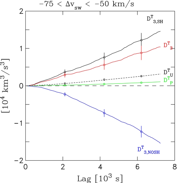
Figure 2. Structure function terms vs. lag for the second leftmost speed bin in Figure 1. The plot shows the contribution from fluctuation and shear terms to the total sum where the sum for shear analysis is DT3, SH (solid black line), fluctuation term is DT3 (solid red line), shear transfer term is DTU (short dashed black line), shear production term is DTP (solid green line), and the no-shear analysis is DT3, NOSH (solid blue line). Error bars included with data points. The time lag used in this plot and following is the spatial lag divided by a wind speed of 400 km s−1.
Download figure:
Standard image High-resolution image
Figure 3. Structure function terms vs. lag for the second rightmost speed bin in Figure 1. Plot quantities rendered as in Figure 2.
Download figure:
Standard image High-resolution imageIn Figure 2, all quantities vary approximately linearly with lag over the plotted range. By far the largest contribution to DT3, SH comes from the detrended third-moment term DT3. The values of DTU and DTP are smaller, with DTU larger than DTP. Though small, DTP has a value that is more than one standard deviation from zero. The relative error for DTP is less than 1%, and the error bars for DTP in Figure 2 are smaller than the plotted symbol size. Its magnitude and sign can be compared to the predictions of shear-driven turbulence. Here, DTP has a positive sign as expected from the generation of energy from the shear. Its relatively small value is consistent with the plotted range of lags being in the inertial range. Since DTP according to Equations (25) and (30) depends on 〈δzI/ORδzTO/I(τ)〉 which we measure to be nonzero at all lag times τ, fluctuations are anisotropic, and this too is consistent with shear-driven turbulence.
In Figure 3 where ΔVSW > 0, we find complicated behavior which is beyond our expectations for homogeneous shear-driven turbulence. In Section 4, we will discuss how compressive effects can contribution to this behavior. The term DT3, SH varies linearly with lag starting from near zero out to about 2000 s, which is in accordance with theory, but then decreases and follows a nonmonotonic course. The linear range is only a quarter of the plotted range and smaller than the expected inertial range. The computed value of TSH is taken only from this range. The term DT3 changes from positive values to negative ones beyond 2000 s. Both DT3, SH and DT3 have values with much larger uncertainty than corresponding points in Figure 2. The term DTU varies nearly monotonically over the whole range which corresponds to increasing fluctuation energy with increasing lag. It even exceeds DT3 beyond lags of 1000 s. The term DTP remains close to zero in the plotted range. The irregular behavior of DT3, SH with lag which is found for all bins with ΔVSW > 0 and its relatively large uncertainty undoubtedly contributes to the scatter about heat in TSH.
In the theory we expect symmetrical results for rarefaction and compression intervals. In Figure 2, we find that the plotted quantities for rarefactions are well behaved with consistent behavior throughout the entire range and measurement uncertainties are relatively small. By contrast, Figure 3 shows for compressions that the plotted quantities do not follow a consistent trend and do not conform to expectations of linear scaling. Therefore, we fail to find the expected symmetry and conclude based on the observed nonlinear scaling and larger uncertainties that the analysis provides a poorer assessment of compression regions.
Because the terms DI/OP provide the most direct measurement of the effects of shear-driven turbulence, we examine separately the underlying fluctuation structure functions. These are the second-order structure functions given by 〈δzI/ORδzO/IT〉. In the theory the sign of 〈δzI/ORδzO/IT〉 matches that needed to produce energy for the cascade. In addition, the absolute value of 〈δzI/ORδzO/IT〉 increases with increasing scale since production is strongest at the large, energy-containing scales. Figure 4 plots 〈δzIRδzOT〉 and 〈δzORδzIT〉 as a function of lag for the ΔVSW bin from −100 to −75 km s−1. Figure 5 plots the same but for the ΔVSW bin from +75 to +100 km s−1.
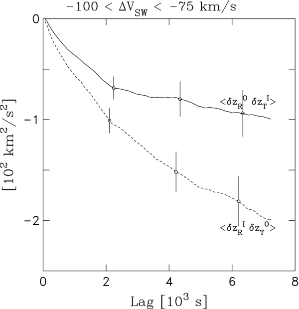
Figure 4. Second-order structure functions vs. lag for the leftmost bin in Figure 1. The values are intrinsic to shear production. Negative values are consistent with shear-driven turbulence. Table 2 gives fit parameters.
Download figure:
Standard image High-resolution image
Figure 5. Second-order structure functions vs. lag for the rightmost bin in Figure 1. Positive values are consistent with shear-driven turbulence. Table 2 gives fit parameters.
Download figure:
Standard image High-resolution imageIn Figure 4, both 〈δzIRδzOT〉 and 〈δzORδzIT〉 have a negative sign consistent with the production of shear-driven turbulence and the magnitude increases with increasing scale, as is expected for driving by shear. Other bins with ΔVSW < −25 km s−1 show the same behavior.
On the other hand, for compressive flow, Figure 5 shows 〈δzIRδzOT〉 and 〈δzORδzIT〉 that are increasing for lags shorter than 2000 s but then are decreasing for larger lags. The sign is positive for shorter lags, consistent with shear-driven turbulence, but can become negative at a large enough lag. This behavior is not found in all bins with ΔVSW > +25 km s−1 wherein 〈δzIRδzOT〉 and 〈δzORδzIT〉 are sometimes found to be negative for all lags. Thereby, results for positive ΔVSW bins continue to show inconsistencies with shear-driven turbulent predictions.
In Figures 4 and 5, power-law fits have been made to quantities as a function of lag. Fit parameters and lag ranges are given in Table 2. The power-law index is roughly 3/4. This is smaller than the expected value of 4/3 based on Lumley's (1967) dimensional analysis of Kolmogorov-like cascade with linear strain (see Section 2.1). Departures from the Kolmogorov prediction at 1 AU are also found by Tessein et al. (2009) for the second-order velocity fluctuation structure function, whereas the corresponding structure function for the magnetic field fluctuation does satisfy the prediction. Thus, the results for 〈δzI/ORδzO/IT〉 may be another manifestation of the velocity fluctuation departure. Potentially, the lack of correspondence with a Kolmogorov cascade indicates that the turbulent state at 1 AU has not yet reached an asymptotic statistically steady state.
Table 2. Fits for Figures 4 and 5
| ΔVSW Range | Quantity | Fit | Lag Range |
|---|---|---|---|
| (km s−1) | (s) | ||
| −100 < ΔVSW < −75 | 〈δzIRδzOT〉 | (− 0.339+0.004 − 0.004)τ0.73 ± 0.01 | 0 < τ < 7232 |
| −100 < ΔVSW < −75 | 〈δzORδzIT〉 | (− 0.479+0.009 − 0.009)τ0.62 ± 0.02 | 0 < τ < 7232 |
| +75 < ΔVSW < +100 | 〈δzIRδzOT〉 | (0.072+0.007 − 0.006)τ0.86 ± 0.10 | 0 < τ < 2048 |
| +75 < ΔVSW < +100 | 〈δzORδzIT〉 | (0.158+0.008 − 0.008)τ0.82 ± 0.06 | 0 < τ < 2048 |
Download table as: ASCIITypeset image
The anisotropy of the fluctuation energy is set by the free parameters b and c where a = 1 without loss of generality, and we now consider how this impacts the mean dissipation rate. Here, we limit the discussion to the two bins with ΔVSW ⩽ −50 km s−1 which are the ones that agree best with homogeneous shear-driven turbulence. Moreover, we only consider varying b, keeping c = 1. We do this because b gives the anisotropy in the plane of the background velocity and gradient, which is the important factor to consider regarding linear shear.
Figure 6 plots TSH as a function of the free parameter b for the ΔVSW bin from −100 to −75 km s−1. A value of b = 1 corresponds to isotropy, and a value of b = 2 corresponds to the 2:1 anisotropy used in the previous plots. The lower dashed line corresponds to heat and the upper dashed line corresponds to 50% above heat, which gives an approximate bound for the additional energy required to heat electrons. For this bin, values of b between 1.06 and 1.69 yield mean dissipation rates in the expected range of plasma heating. For the next adjacent ΔVSW bin which ranges from −75 to −50 km s−1 (not shown), b = 1 has TSH slightly greater than heat, while 50% excess is reached for b = 1.69. Thereby, for these bins modest amounts of anisotropy are consistent with plasma heating.

Figure 6. Plot of mean dissipation rate vs. in-plane fluctuation energy anisotropy parameter b for the leftmost bin in Figure 1. Departure of b from 1 indicates the amount of anisotropy. Lower dashed line corresponds to = heat and upper to = 1.5heat.
Download figure:
Standard image High-resolution image3.2. Sorting Results by VSWTP
In the present analysis based on the WSOM equations, we have modeled the anisotropy induced by the velocity shear on the fluctuations. Anisotropy associated with the direction of B0 has not been considered here.
Previous studies (MacBride et al. 2005, 2008; Stawarz et al. 2009, 2010) employed data that were selected without regard to shear and therefore averaged over approximately equal amounts of increasing and decreasing shear regions, as is required for this approach. These studies found that the PP equations give mean dissipation rates that could account for expected proton heating rates. In order to determine how the results using the WSOM equations compare with these previous studies, we perform the Stawarz et al. (2010) analysis for bins of VSWTP using Equations (32)–(35) which correspond to the isotropic fluctuation formalism in their paper. Stawarz et al. (2010) also obtained rates parallel and perpendicular to B0 whose sums are in better agreement with the expected total plasma heating than the rates based on the isotropic case. Here, we only compare with the isotropic case since the shear formalism does not yet include additional anisotropy effects associated with B0.
In accordance with Stawarz et al. (2010), 12 hr intervals are placed into seven overlapping VSWTP bins based on the average product of the solar wind velocity and the proton temperature within the interval. For each of the VSWTP bins, we again compute TSH with a 2:1 anisotropy, TNOSH, and heat using the methods described above.
Figure 7 plots these three quantities against the average value of VSWTP within each bin, and values are given in Table 3. Although the shear is considered in calculating TSH for each 12 hr interval, values are only averaged in Figure 7 by VSWTP bins. Compressions and rarefactions occur in all bins. Note that due to a small error in the selection of 12 hr intervals in the Stawarz et al. (2010) analysis and new selection criteria in applying the shear formalism, the values plotted for TNOSH are slightly different from those shown in Stawarz et al. (2010). The same conclusions that were drawn in Stawarz et al. (2010) can, however, be inferred from the slightly revised data. All quantities in Figure 7 tend toward larger rates for increasing VSWTP. The value of TSH trends from above heat in the two lowest VSWTP bins to below heat in the highest bins. The value of TNOSH deviates from heat in the opposite sense.
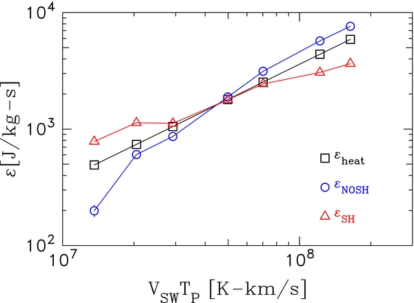
Figure 7. Reanalysis of Stawarz et al. (2010) plotting mean dissipation rate vs. VSWTP for 12 hr intervals and comparison with the average proton heating rate. Error bars are smaller than symbols. Table 3 gives the plotted data values, errors, and sample numbers.
Download figure:
Standard image High-resolution imageTable 3. Rates for Figure 7
| VSWTP Range | Number of | TSH |
TNOSH |
Theat |
|---|---|---|---|---|
| (× 107 km s−1 K) | Samples | (× 103 J kg−1 s−1) | ||
| 0.2 < VSWTP < 2.0 | 978 | 0.78 ± 0.03 | 0.20 ± 0.02 | 0.49 ± 0.00 |
| 1.1 < VSWTP < 3.0 | 1536 | 1.13 ± 0.04 | 0.60 ± 0.03 | 0.73 ± 0.01 |
| 2.0 < VSWTP < 4.0 | 1446 | 1.12 ± 0.05 | 0.86 ± 0.04 | 1.05 ± 0.01 |
| 3.0 < VSWTP < 8.0 | 1851 | 1.78 ± 0.04 | 1.89 ± 0.03 | 1.79 ± 0.01 |
| 4.0 < VSWTP < 12.0 | 1814 | 2.44 ± 0.04 | 3.13 ± 0.04 | 2.52 ± 0.02 |
| 8.0 < VSWTP < 26.0 | 991 | 3.06 ± 0.07 | 5.71 ± 0.07 | 4.39 ± 0.04 |
| 12.0 < VSWTP < 40.0 | 413 | 3.65 ± 0.15 | 7.63 ± 0.15 | 5.88 ± 0.07 |
Download table as: ASCIITypeset image
Stawarz et al. (2010) noted that the two lowest bins of VSWTP contain intervals mainly from the lower temperature extremes of the solar wind. Following Vasquez et al. (2007), they suggested that heat may be overestimated in these lower bins because the analyses for heat only considered VSW selection to obtain the radial proton temperature gradient. Freeman & Lopez (1985) found that cold intervals at 1 AU are more consistent with nearly adiabatic behavior. This differs significantly from the average behavior based on VSW. Thereby, the deviations in the lower bins for TNOSH were not considered detrimental to the analysis of TNOSH, at least with the current knowledge of heating rates.
The two highest bins of VSWTP have TNOSH greater than heat. Stawarz et al. (2010) found that these intervals mostly come from fast winds that always have high TP. Electron heating has been noted by Pilipp et al. (1990) for fast winds and there is no discernible heating in slower wind intervals. The trend from TNOSH near heat for the lower bins of VSWTP to TNOSH greater than heat at the highest bins is then consistent with the expectations for total plasma heating.
Two concerns are then evident about the values of TSH as a function of VSWTP. For the two lowest VSWTP bins, TSH certainly provides sufficient energization for proton heating. Are these values too high even for total plasma heating? Additionally, in the two highest bins, TSH is too small to explain even proton heating.
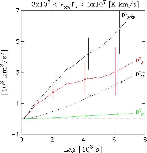
Figure 8 plots DT3, DTU, DTP, and DT3, SH as a function of lag for the middle VSWTP bin. As expected, DT3, SH is approximately linear with respect to lag. The term DT3 provides the dominant contribution to the total DT3, SH. These results are typical of all VSWTP bins except for the two largest bins where DTU begins to dominate the sum at long lags. Recall that DTU dominance at longer lags is a feature of ΔVSW > 0 intervals (see Figure 3). Combine this with the fact that TSH is not well determined for ΔVSW > 0 and that intervals with ΔVSW of both signs are mixed together in VSWTP bins, and we surmise that intervals with ΔVSW > 0 are a likely contributor to the lack of agreement between TSH and heat. Moreover, the highest bins of VSWTP contain relatively more intervals of large positive ΔVSW and thus strong compression regions.
Figure 8. Structure function terms vs. lag for the shear analysis where VSWTP is near the middle of the plotted range in Figure 7. Corresponding plot quantities rendered as in Figure 2.
Download figure:
Standard image High-resolution image
4. DISCUSSION
For homogeneous shear flow, the sign of the shear gradient should have no influence on the mean dissipation rates. Rather, only the magnitude of the shear contributes. This is clearly not found in the analyses of the ACE data. Rising VSW time intervals do not predict the same dissipation rate as the corresponding falling intervals. Moreover, the predicted linear trend of total modified third moments DT3, SH in rising intervals is only achieved on a relatively short range of time lags smaller than the expected inertial range.
The most probable reason for the difference is the importance of compressional flow near sharply rising VSW intervals. Corotating interaction regions where slow wind is overtaken by fast wind have been simulated with MHD numerical codes (see Gosling & Pizzo 1999 for a review). The simulation results show that the velocity is compressional in the interaction region in that the velocity is deflected from the radial direction and has gradients normal to the stream interface with components along the radial direction, as well as along the tangential and northward directions. This means that the background flow near the interaction region is not consistent with a homogeneous shear flow.
The differences between the actual flow and the assumed homogeneous shear flow appear to be too great to apply the present analyses accurately. The linear behavior of the structure functions at small lags for rising intervals suggest, however, that the fluctuations are noncompressive at these same scales. The background velocity may then require the most attention and would at least involve calculating the shear based on a determination of the actual orientation of the stream interface. In the present analyses, the normal to this surface has been assumed to be along the  direction so that α is then generally underestimated for rising intervals.
The falling VSW intervals correspond to extensive rarefactions which have rather gentle gradients of background plasma density. Conditions here are closer to ones matching a homogeneous shear flow. We find that DT3, SH is linear over a considerable range of lags. Dissipation rates can be determined which are consistent with plasma heating rates. Thereby, the approach of homogeneous shear flow is better with rarefaction intervals.
The difference between rising and falling intervals impacts the analysis of dissipation rates versus proton heating as a function of VSWTP. When the analysis is made with regard to shear-dependent terms, the dissipation rates fall below observed proton heating rates for the two largest VSWTP bins. These bins contain the highest percentages of high-speed winds and intervals of large rising VSW. The inconsistency here is likely ascribed to the relative strength of compression in the rising speed intervals and its impact on the shear analysis. On the other hand, third-moment analysis without velocity detrending which combines rising and falling intervals finds dissipation rates in accord with observations in these same bins.
5. SUMMARY
We have obtained moments from a large set of ACE data and examined 6 and 12 hr intervals with the exclusion of known interplanetary shock intervals and magnetic cloud intervals. Moments are interpolated to a common spatial lag grid and behavior examined out to lags of ∼2 hr based on a reference speed of 400 km s−1. Lags in this range correspond to values expected for the inertial range of fluctuations in the solar wind.
Moments are compared with the results from incompressible MHD for homogeneous fluctuations. When the total velocity is considered with no detrending of the background velocity shear, the PP equations, given by Equation (33), are used to determine dissipation rates assuming isotropy. Since stationary conditions are assumed, the mean dissipation rate is equivalent to the cascade rate of the turbulent energy. These equations predict that the third moment for outward and inward Elsässer components varies linearly with lag. The average of the outward and inward third moments, called the total third moment DT3, NOSH, is proportional to the mean dissipation rate.
When the velocity shear is detrended from data, the WSOM equations, given by Equation (22), for MHD homogeneous shear flow turbulence are used. In the WSOM equations, the modified third moments for each of the outward and inward components are expressible as the sum of a fluctuation-only inertial range transfer term and two shear dependent terms. One shear term involves transfer in the inertial range, and the other involves production that is most significant in the energy-containing range. The sum of individual terms in each WSOM equation is linear with lag. The total modified third moment DT3, SH is proportional to the mean dissipation rate.
The background solar wind flow is taken to be in the radial direction from the Sun, which is largely true. Gradients across this flow are not directly measured by a single spacecraft. As the solar wind convects past the spacecraft, different sources of wind are, however, brought to bear by the rotation of the Sun. The velocity gradient, given by Equation (36), is then determined from the ratio of the change of the linearly detrended background velocity for the interval time and the distance along a heliocentric circular arc traversed at 1 AU due to solar rotation for the same amount of time. Moreover, the gradient is assumed to be along the direction of solar rotation. As such, the shear is contained in the RT plane. In this approach, the tilt of the shear out of this plane is neglected, and the flow is assumed to be incompressible.
Another essential aspect to the approach using the WSOM equations concerns the fluctuation anisotropy which cannot be directly assessed using single-spacecraft techniques. Therefore, a set of approximations is used for the terms in the WSOM equations so that they are re-expressed using observed quantities and free parameters for fluctuation anisotropy. The assumed fluctuation anisotropic energy distribution averaged over lag was developed based on the behavior of vortex stretching of eddies associated with shear-driven turbulence. The assumed form of the anisotropy most strongly impacts the estimation of the shear transfer terms. The range of the free parameters is limited to values where mean dissipation and expected plasma heating rates are in acceptable agreement.
With data selection emphasizing velocity shear, the evaluation of the mean dissipation rate using the PP equations and no velocity detrending finds approximately linear behavior for DT3, NOSH with lag. The sign of DT3, NOSH has, however, the same sign as the shear, and DT3, NOSH yields a value of the mean dissipation rate that is not in agreement with the heating rate. This behavior is consistent with the need to apply the PP equations only to cases where the average shear is near zero.
When the same data are evaluated using the WSOM equations and assuming an anisotropy of 2:1 in the RT plane, linear scaling for DT3, SH was found for the entire range of lags for intervals of falling VSW. The range, however, was much smaller and confined to the smaller lags when VSW rises. From these linear portions, mean dissipation rates were obtained. These have positive values regardless of the sign of the shear and so are consistent with a forward energy cascade that at small scales would dissipate and heat the plasma.
As the magnitude of the shear increases, the mean dissipation rate generally increases, and so does the proton heating rate. This is also consistent with shear-driven turbulence because the production of energy is proportional to the magnitude of the shear. These results are in apparent contradiction with the recent work by Borovsky & Denton (2010).
The trend of the mean dissipation rates is, however, only rigorously followed for falling VSW intervals, while the rising VSW intervals contain more scattered and less certain values for rates. The observations further show that there is a lack of one-to-one correspondence between falling and rising intervals of equal magnitude regarding mean dissipation rates and the extent of the linear range of lags for DT3, SH. This is inconsistent with the predictions based on homogeneous shear flow for which the sign of the shear does not affect the above quantities. In the solar wind, the rising intervals correspond to compression regions and the falling intervals to rarefaction regions. The deviations from the predictions of homogeneous shear flow are much larger for the compression regions. This is to be expected based on the development of corotating interaction regions. Thus, shear analysis which assumes incompressible flow is better performed for the rarefaction regions rather than for the compression regions.
The WSOM formalism provides an assessment of the relative contribution of three total terms to the mean dissipation rate when homogeneous velocity shear is present. Confining this assessment to the falling VSW intervals with significant shear magnitude, we find in the solar wind that of the two terms that we can calculate more directly, the total production term DTP in Equation (29), arising from the cross-correlation of the detrended fluctuating components in the RT plane, is negligible compared to the third moment of the detrended fluctuations DT3 in Equation (27). The small relative value of DTP is consistent with a value expected from the inertial range. The estimate of the remaining total shear transfer term DTU in Equation (28), which arises from shear-induced anisotropy in the second moment, is also less than DT3. For all terms, anisotropy less than 2:1 yields a mean dissipation rate consistent with the expected plasma heating rate. The required amount of shear-induced anisotropy is then small.
In addition to the above, the production terms provide direct measurements that test the predictions of velocity shear-driven turbulence. Its nonzero value is more than one standard deviation from zero and thus is consistent with the presence of fluctuation anisotropy, which velocity shear is expected to produce. Its sign is found to be consistent with a shear-driven forward turbulent energy cascade. The scaling of the cross-correlations, which are second moments, that underlie the values of the shear production terms vary, however, less with lag than is expected from a generalization of the dimensional analysis of Lumley (1967). This corresponds to a spectrum for the cross-correlation that is flatter than the same spectrum associated with a Kolmogorov-like energy cascade. This finding is consistent with the lack of correspondence at 1 AU of the total energy and velocity spectrum to the Kolmogorov form.
A final analysis was carried out to determine the mean dissipation rate as a function of the product of solar wind speed and proton temperature VSWTP, which is proportional to the proton heating rate (Gazis & Lazarus 1982; Gazis et al. 1994; Totten et al. 1995). In this case, the sorting of intervals is not according to velocity shear and thus combines rising and falling VSW intervals so that the average shear is near zero. This favors the approach using the PP equations. When third moments are determined without detrending velocity, mean dissipation rates from the PP equations can match or exceed expected proton heating rates as a function of VSWTP. In particular, for the largest values of VSWTP, this approach obtains mean dissipation rates greater than proton heating rates which are to be expected based on additional electron heating present in fast winds.
The corresponding analysis carried out with shear terms leads to rates that can match proton heating rates for the middle ranges of VSWTP. However, the mean dissipation rates are too small at the largest values of VSWTP even to account for proton heating alone. This latter discrepancy likely indicates that improvements are needed to the shear approach to determine accurately rates from compressional, rising VSW intervals.
The authors thank the ACE/SWEPAM team for providing the thermal proton data used in this study. J.E.S. and C.W.S. are supported by Caltech subcontract 44A1085631 to the University of New Hampshire in support of the ACE/MAG instrument. C.W.S., B.J.V., and M.A.F. are supported by NASA Sun–Earth Connection Guest Investigator grants NNX08AJ19G and NNX09AG28G. B.J.V. is also supported by NSF SHINE grant ATM0850705 and NASA Solar and Heliospheric Physics SRT grants NNX07AI14G and NNX10AC18G. J.E.S. is an undergraduate physics major at the University of New Hampshire.