


ABSTRACT
The addition and incorporation of highly ordered distributions of pickup ions can increase the ordering of space plasmas, decreasing their entropy, and driving them away from equilibrium. In this study, we present a model for describing the entropy decrease of heliospheric plasmas caused by the pick-up ions and their highly ordered arrangement. We consider a plasma flow consisting of two proton populations: (1) a solar wind distribution that is in quasi-equilibrium and (2) a spherical shell distribution of pick-up protons. Because all protons are indistinguishable, they equally share a hybrid state, where the hybrid probability distribution is given by the normalized sum of the distributions of the solar wind and pick-up protons. We derive an analytical formulation of the thickness of the pick-up proton shell distribution. Then we show that the entropy of the hybrid state depends on a dimensionless fluctuation number, Θ, which is a measure of the organizing role of pick-up protons. This number characterizes and compares two types of fluctuations, the thermal motion of solar wind protons and the bounded motion of pick-up protons that forms the spherical shell distribution. We find that the entropy variation between the hybrid and original states is proportional to the negative logarithm of Θ. When the two competing fluctuations balance each other, Θ ∼ 1, the pick-up protons have no effect on the entropy of solar wind protons. Remarkably, while sunward of the termination shock pick-up ions act to slightly increase entropy, throughout the inner heliosheath their effect is to decrease the entropy dramatically.
Export citation and abstract BibTeX RIS
1. INTRODUCTION
The solar wind expands outward through the heliosphere and interacts in multiple ways with both itself and the plasma of the Local InterStellar Medium (LISM). Pick-up protons are created in the outer heliosphere, mostly via (1) charge-exchange interactions between the LISM hydrogen atoms and solar wind protons or/and (2) photoionization of the former by solar extreme-ultraviolet (EUV) radiation. In particular, neutral hydrogen atoms that originate in the LISM can penetrate deeply into the heliosphere and undergo either a charge-exchange interaction with the solar wind protons or photoionization, respectively, according to

The rate of (1) is roughly one order of magnitude larger than that of (2) for hydrogen/protons (see Rucinski et al. 1996). Hereafter we focus on the influence of pick-up protons on the bulk space plasma that is the solar wind protons sunward of the termination shock and the inner heliosheath.
The neutral hydrogen atom produced (1) continues to propagate inside the heliosphere following the solar wind flow (S) and its bulk velocity  , is unimpeded by any electromagnetic field interaction. On the other hand, the protons produced from either (1) or (2) initially inherit the bulk velocity of the LISM flow (L), i.e.,
  , and interact with the interplanetary magnetic field
  . In the reference frame of the solar wind flow, the relative velocity of the proton is
  , and because its direction typically does not coincide with the magnetic field vector, the proton gyrates around the magnetic field
  . In this way, the proton produced which originates from the neutral hydrogen of the LISM is picked up by the solar wind flow with an initial gyrospeed that equals
  , because
  , where
  ,
,  and ⊥ means the projection on the direction of
  .
.
After ionization, the picked-up proton's initial gyrospeed has a constant magnitude wPUI. Hence, the values of velocities of the picked-up protons are distributed in a ring of radius wPUI in the three-dimensional velocity space and centered at the solar wind velocity. This ring is quickly transformed into a spherical surface, with approximately the same center and radius wPUI, due to scattering that does not affect the energy of the pick-up protons, e.g., by self-generated Alfvénic fluctuations (Sagdeev et al. 1986; Lee & Ip 1987). Subsequently, fluctuations of the velocity wPUI of the pick-up protons can gradually transform the spherical surface of velocities into a spherical shell distribution of thickness Δw (Zank 1999).
While the physical meaning of the radius wPUI of the spherical shell distribution is well understood, the origin of the fluctuations of velocities that produces the thickness Δw of the shell is not so trivial. It is a challenge to interpret and reach a physically meaningful value for this thickness, 0 < Δw ≪ wPUI. It is notable that in previous studies the value of Δw was appropriately handled so that its actual value was avoided, e.g., in the work of Heerikhuisen et al. (2010) that examines the pick-up protons of the outer heliosheath as a possible source of the ENAs detected by IBEX (McComas et al. 2009a, 2009b, 2010), the thickness Δw was related to the specified energy window ΔE of the instrument counting energetic neutral atoms (ENAs), wPUIΔw ≈ ΔE/μ (μ is the proton mass).
The solar wind protons without the addition of the pick-up protons are well described by kappa distributions (see Livadiotis & McComas 2009, 2010a, and references therein). These involve a certain generalization of the Maxwellian distribution (Maxwellians exclusively characterize systems at thermal equilibrium). The kappa index (indicated by the Greek letter "κ"), which parameterizes these distributions, labels the specific stationary state out of equilibrium in which the system resides. The range of all possible values of the κ-index corresponds to an arrangement of stationary states lying between equilibrium, having a maximum value of κ → ∞, and the furthest state from equilibrium that is characterized by the minimum value  .
.
The solar wind together with pick-up protons are characterized by a hybrid probability distribution. This is the normalized sum of the probability distribution of the original stationary state of the solar wind protons (the initial kappa distribution) and the spherical shell distribution of the pick-up protons. Potentially, it describes a more organized state having lower entropy than the stationary state assigned by the original probability distribution of the solar wind, before the inclusion of pick-up protons.
The solar wind generally refers to the stream of particles accelerated out of the solar corona. However, in its continuing flow outward through the heliosphere, it is continuously enriched with pick-up ions. After enough time, the pick-up ions are incorporated into the original solar wind, which then has a single, indistinguishable distribution, which is a kappa distribution with a new kappa index (Livadiotis & McComas 2010a). Throughout the paper, we refer to this simply as "solar wind," by which we mean the "pick-up ion incorporated solar wind" and not the solar wind coming directly out of the corona. The incorporated solar wind protons are also referred to as either original solar wind protons or bulk solar wind protons in order to separate them from the newly formed pick-up protons.
The organizing role of pick-up ions in the solar wind is of great importance because the associated decrease in entropy leads the system far from thermal equilibrium (Livadiotis & McComas 2010a). In their co-motion with the solar wind in the heliosphere, pick-up protons undergo adiabatic cooling that reduces the radius of the shell (Zilbersher & Gedalin 1997). Ultimately, pick-up protons move from the shell distribution and merge with the solar wind protons into a new kappa distribution (Figure 1). This characterizes a new stationary state with lower entropy than the initial one. Far from equilibrium the stationary states are typically characterized by entropy lower than that near equilibrium (Livadiotis & McComas 2010a, 2010c). Hence, the new stationary state can be described by a kappa distribution with a κ-index smaller than its initial value and closer to the furthest state limit of  . Following this, in the distant solar wind of the outer heliosphere, where pick-up protons represent an increasing fraction of the population, the entropy may become smaller as the plasma transits to stationary states further from equilibrium that have lower entropy. The pick-up ion effect leads to stationary states far from equilibrium.

Figure 1. Transition of space plasmas in near equilibrium stationary states is characterized by monotonic entropic behavior. As the entropy decreases, the κ-index also decreases and the system is diverted further from equilibrium. Solar wind protons, p+(S), residing in a stationary state with kappa-index κ1 and entropy S1, are mixed with pick-up protons, p+(PUI), forming the hybrid state of indistinguishable protons, [p+(S)  p+(PUI)]*, which finally degenerates into a new stationary state with kappa index κ2 and entropy S2.
Download figure:
Standard image High-resolution imageThis paper is organized as follows. In Section 2, we examine the radial thickness of the spherical shell distribution of pick-up protons. In Section 3 we introduce the "fluctuation number" by volume, Θv, and by density, Θd, which characterize pick-up protons and their spherical shell distribution. In Section 4, we construct the probability distribution that describes the hybrid state of the solar wind and pick-up protons. Then, the influence of pick-up protons on the entropy is analytically developed. In Section 5 we examine how the fluctuation number is distributed in the heliosphere, and we discuss the implications for the entropy and the κ-index. Finally, Section 6 summarizes the primary results of this study and provides some conclusions. Appendix A derives the thickness of the spherical shell distribution of pick-up protons; Appendix B calculates the entropy variation ΔS and shows how this depends on the fluctuation numbers.
2. THICKNESS OF THE SPHERICAL SHELL
If a is the pitch angle of the solar wind protons, which is between  and the local interplanetary magnetic field
  , then the pick-up proton gyrates around
  approximately with a velocity of
  . Taking into account the bulk velocity of the LISM flow
  , the exact pick-up proton initial velocity
  does not coincide with the solar wind bulk velocity
  , either in magnitude or direction, exhibiting a small angle ϑ between their vectors,
  and
and  (see Figure 10 in Appendix A). The pitch angle of the pick-up protons, i.e., aPUI = a + ϑ, gives the direction of the pick-up protons' initial velocity,
  , with respect to the direction of the magnetic field
  . This velocity in the heliospheric reference frame is
  , while in the bulk solar wind frame it is
  , where the ring radius is

This is the spherical shell radius of the pick-up proton distribution, while variations of this radius contribute to the thickness of this shell, Δw.
In Appendix A (see (A7)) we calculate the thickness Δw of the spherical shell expressed in terms of the solar wind bulk velocity  and the longitude from the nose φ, as well as of the average pitch angle,
  , and its deviation δa, i.e.,
  .
.
The direction of the local interplanetary magnetic field  is on average roughly perpendicular to the solar wind flow and its bulk velocity
  (a = 90°). In general, however, the solar wind bulk velocity and the interplanetary magnetic field are subject to strong and complicated variations. Fluctuations of the angle a which constitute an angular deviation δa from an average value
  can also contribute to the thickness of the spherical shell (Zank 1999).
We start examining the thickness by considering the simple case of  . In Figure 2 we show the dependence of
  on the velocity ratio
  and the longitude φ (for δa = 5°). In particular, in Figure 2(a) we depict
  in terms of
  and for various longitudes (φ = 0°, 15°, 30°, 45°, 60°, 75°, 85°, 90° and its supplementary angles). We note that for values of
  greater than ∼20 (slightly dependent on φ), the thickness is stabilized to a certain value depending on φ. The realistic values of the ratio
  range from ∼10 to ∼40. However, our graph covers a wider range,
  , to make clearer the thickness asymptotic behavior for large solar wind velocities. In Figure 2(b) we depict
  in terms of the longitude φ and for various values of
  (2, 3, 5, 10, and 100). The thickness varies from its maximum value
  (for φ = 0°, 180°) to its minimum value
  (for φ≅90°, 270°). While the maximum value is always
  , independent of the value of
  , its minimum value is slightly dependent. The longitude φMin for which the minimum thickness appears also depends on
  ; for small values of
  , the value of φMin is slightly larger than 90° (slightly smaller than 270°), while for larger values of
  this tends to be exactly 90° (270°).

Figure 2. Thickness of the spherical shell,  , depicted for the simple case of pitch angle
  (δa = 5°), as a function (a) of the solar wind bulk velocity
  , for longitudes φ = 0°, 15°, 30°, 45°, 60°, 75°, 85°, 90° (solid lines) and its supplementary angles (dash-dot lines) and (b) of the longitude φ, for velocities
  = 2, 3, 5, 10, 100. (All the velocities are expressed in terms of the LISM bulk velocity
  .) (c) The minimum thickness that appears for longitudes ∼90° and ∼270° (panel b) depicted as a function of
  which is almost constant for
  >10 and equal to δa≅5°≅0.0873 rad. Note that when
  , the thickness takes bounded values,
  (see text and Appendix A).
Download figure:
Standard image High-resolution imageThe dependence of the minimum thickness on  , i.e.,
  , is shown in Figure 2(c). We observe that
  decreases monotonically and for large values of
  , this tends toward a limit value of
  that coincides with δa≅5°≅0.0873 rad. This is the smallest possible value of the thickness. It can be easily shown analytically that the maximum and minimum values of the thickness are
  (φ = 0°) and
  (φ = 90°), respectively (see Appendix A). Therefore, when
  , the thickness can take values in the interval
  .
.
The thickness minimum value is interesting since it indicates where there may be large decreases of entropy. The smaller the minimum is, the more organized the pick-up protons are, and the more effective they are in decreasing the entropy of the solar wind. Hence we investigate the specific parameter values that determine the thickness minimum. As we will see, in the case of  (but with
  being close to 90°), the minimum (or minima) of thickness may become much smaller than δa.
The functional behavior of the thickness is extremely different when the orientation of the pick-up proton velocity and the magnetic field are not at right angles ( ). For instance, the dependence of the thickness on the longitude is symmetric on the reflection φ → −φ, only for
  (and all multiples of 90°, i.e., 0°, 90°, 180°...), while this symmetry breaks as the average angle
  deviates from a right angle. Certainly, the thickness is symmetric to the double transformation
  , φ → −φ.
In Figure 3 we depict the thickness  as a function of the velocity ratio
  for longitude φ = 90°, pitch angle deviation δa = 10°, and various values of the pitch angle,
  . We observe that for reasonable values of the solar wind velocity, that is, for values of the ratio
  from ∼10 to ∼40, the thickness typically increases with the solar wind bulk velocity. Precisely, however, there is a minimum (for
  ); in most of the cases this is located in the region
  , which is slower than the solar wind. The minimum is meaningful when the pitch angle is very close to ∼90°. Therefore, for values of the pitch angle of
  (that is, specifically for φ = 90°, δa = 10°) the minimum of
  appears in the interval
  .
.

Figure 3. Thickness of the spherical shell,  , depicted as a function of the solar wind bulk velocity,
  , for longitude φ = 90°, pitch angle deviation δa = 10°, and various values of the pitch angle,
  . The thickness has a non-monotonic behavior as a function of the solar wind bulk velocity,
  . This function is convex, exhibiting a minimum. The minimum can appear for reasonable values of the solar wind velocity, that is, for values of the ratio
  from ∼10 to ∼40. For example, in the present case of φ = 90° and δa = 10°, the minimum is located in the interval
  for values of the pitch angle
  . Otherwise, the thickness decreases or increases monotonically in the interval
  , for values of the pitch angle
  or
or  , respectively. Note that generally, the maximum of the thickness is not bounded by the LISM bulk velocity, in contrast to the case of
  , where we have
  (as demonstrated in Figure 2).
Download figure:
Standard image High-resolution imageFigure 4 shows the longitude dependence of the thickness on the equatorial plane in polar coordinates and for various pitch angles  (columns) and deviations δa = 5°, 10° (rows). For each panel we depict the thickness for four values of solar wind bulk velocity,
  . We observe that the thickness increases with the deviation δa; the scale in the second row (δa = 10°) is double that in the first row (δa = 5°). For
  , the thickness forms a curve with a shape of a "lying 8" having two minima for longitudes ∼90° and ∼270°, as showed in Figure 2(b). As the pitch angle decreases, these minima become weaker, while the curves for different velocities become farther from each other. The minimum thickness at φ ∼ 90° is smaller than that at φ ∼ 270°, but this asymmetry occurs since we depict pitch angles
  . For
. For  we have the symmetrical diagrams (for the relation φ → −φ), i.e., the minimum thickness at φ ∼ 270° would be smaller than that at φ ∼ 90°. Finally, we note that the thickness can increase with the solar wind bulk velocity without any upper limit, as when
  where there is a maximum thickness
  when φ = 0° or 180°.

Figure 4. Thickness of the spherical shell,  , depicted as a function of the longitude φ on the equatorial plane in polar coordinates, Δw = Δw(φ). The panels in each column are characterized by a different pitch angle,
  (1st column), 80° (2nd column), 85° (3rd column), 90° (4th column), while in each row they have a different deviation, δa = 5° (upper row) and 10° (lower row). In each panel we depict the thickness for four values of solar wind bulk velocity,
  = 10 (red solid), 20 (blue dot), 30 (green dash), 40 (purple dash-dot). Note that in the second row (δa = 10°) the scale is double that in the first row (δa = 5°) because the thickness increases with the deviation δa.
Download figure:
Standard image High-resolution image3. CHARACTERISTIC FLUCTUATION NUMBERS BY VOLUME AND DENSITY
3.1. Basic Physical Quantities
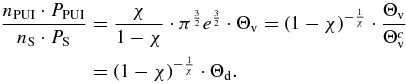
Both populations of protons in the solar wind flow, namely, the original solar wind and the pick-up protons, can be separately characterized by their particle densities, nPUI and nS, as well as by the fractions, χ ≡ nPUI/(nS + nPUI) and the complementary 1 − χ = nS/(nS + nPUI), respectively. We utilize these normalized fractions to quantitatively express the pick-up protons in the solar wind flow, especially for constructing the hybrid probability distribution (next section).
Another characteristic quantity of the pick-up proton population is the volume of the spherical shell distribution in the three-dimensional velocity space, VPUI = 4πw2PUIΔw. The larger this volume is, the more fluctuations the pick-up protons experience, and thus, the less effective an organizing role they have. However, we will see that the organizing pick-up protons have more influence when the original solar wind protons are not well organized by themselves, that is, when the solar wind thermal fluctuations are strong (higher temperature).
Temperature is a crucial parameter for characterizing entropy. Solar wind protons are well-described by kappa distributions. In this formulation the temperature is usually expressed in terms of the effective speed-scale parameter θ, which is simply the temperature in dimensions of velocities, i.e.,

where kB is the Boltzmann's constant, and μ and T are the mass and temperature of the solar wind protons, respectively. Here, with T, we denote the kinetically defined temperature (second statistical moment of velocities). This coincides with the thermodynamic definition of temperature, called "physical temperature," as given and developed in the framework of non-extensive statistical mechanics that generalizes the classical Boltzmann–Gibbs statistical mechanics (Livadiotis & McComas 2009).
The pick-up protons are subject to fluctuations, whose characteristic volume in three-dimensional velocity space is given by the volume of the spherical shell VPUI. On the other hand, the solar wind protons are subject to thermal fluctuations represented by the standard deviations  (here we used the reference frame of the bulk flow
  , in which the velocity of the solar wind protons is
  ). The characteristic volume VS of the thermal fluctuations of solar wind protons is defined to be the volume of the cube with length equal to
  . Hence, VS = θ3.
Below we show how the above parameters are involved in quantifying the organizing role of pick-up protons and the change in entropy. We develop two dimensionless numbers that can measure the organizing role of pick-up protons. These characterize and compare the two types of fluctuations that compete in the change in entropy: the thermal motion of bulk solar wind protons and the bounded motion of pick-up protons that forms the spherical shell distribution. The first number is related to the volume of these fluctuations in the velocity space, and eventually leads to the definition of the second number which is related to the phase space densities of these fluctuations.
3.2. Characteristic Fluctuation Number by Volume, Θv
Here we define a dimensionless quantity Θv that characterizes the organizing role of pick-up protons in the solar wind. This quantity has to be proportional to VS (i.e., increasing with the temperature θ), and inversely proportional to VPUI.
Indeed, a larger volume of the pick-up proton spherical shell, VPUI = 4πw2PUIΔw, signifies larger fluctuations, and thus less effective organizing pick-up protons. However, their organizing character is not absolute, but rather has to be described in comparison with the initial organization of the solar wind protons. When these protons have low temperature, their thermal fluctuations are weak and their characteristic volume VS = θ3 is small. In other words, they are already well organized by themselves, and the pick-up protons are less effective in increasing the order of the system, and thus, in decreasing its entropy. In contrast, for high temperatures, the solar wind protons are subject to strong thermal fluctuations with large characteristic volume VS, and thus, the pick-up protons have much more impact on increasing the order of the system and decreasing its entropy.
We define the quantity Θv to be given by the dimensionless ratio Θv ≡ VS/VPUI. Hence,
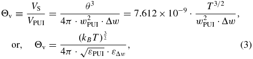
where  and
and  . Note that for aPUI ∼ 90° (e.g., for
  and φ ∼ 0°) we have
  and thus
  .
.
The dimensionless quantity Θv compares the two competing fluctuations of (1) the thermal motion of the bulk solar wind protons and (2) the bounded motion of the pick-up protons. When the former dominates the latter, that is, for large values of Θv, the organizing role of pick-up protons is more effective. This justifies the name given to Θv, which is the fluctuation number. Since we describe the fluctuations by their characteristic volumes in the velocity space, we call Θv the fluctuation number by volume.
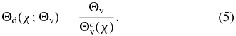
For any given value of the fraction χ of the pick-up protons in the solar wind flow, there is a critical value of the fluctuation number, Θcv, for which the average entropy (entropy per particle) of the system neither decreases nor increases (isentropic influence). In this case, we say that the two competing fluctuations are "entropically equivalent." For greater values of the fluctuation number, Θv > Θvc, the entropy decreases, because pick-up protons add order to solar wind protons and their influence has an effective organizing role in the hybrid state. However, for smaller values of the fluctuation number, Θv < Θvc, the entropy increases, because pick-up protons are less organized than solar wind protons.
The critical value of the fluctuation number depends on the fraction χ of the pick-up protons in the solar wind flow, namely, Θcv = Θvc(χ). For example, when this fraction is smaller than ∼10% (χ < 0.103), the fluctuation number must be Θv > 1 for the entropy to decrease, namely, Θcv(χ = 0.103)≅1. When the fraction χ is 10 times smaller (less than ∼1%), then the fluctuation number has to be 10 times larger, Θv > 10, for the entropy to decrease, namely, Θcv(χ = 0.0108)≅10. In general, we find that for small values of the fraction χ, the critical fluctuation number is inversely proportional to this fraction, i.e., Θcv(χ)∝1/χ. Indeed, in Appendix B we prove the relation
which for small fractions χ is approximated to

Figure 5 illustrates Θcv(χ), for small fraction values χ ≪ 1 (Equation (4b)) and also for any non-small values 0 < χ ⩽ 1 (Equation (4a)).

Figure 5. Critical fluctuation number (by volume), Θcv(χ), depicted as a function of the fraction of pick-up protons χ (log–log scale). For small fractions χ ≪ 1, this behaves like Θcv(χ)∝1/χ (Equation (4b)), that is the linear part of the graph (green dot line), while for arbitrary non-small values, this is concave (Equation (4a)).
Download figure:
Standard image High-resolution image3.3. Characteristic Fluctuation Number by Density, Θd
The sign of the variation of the (average) entropy ΔS between the hybrid state and the original stationary state of the solar wind protons is given by


The definition by volume, Θv, has been defined by the ratio between the characteristic volumes of the two competing fluctuations of the solar wind thermal motion and the bounded variation of the pick-up protons (3). Unfortunately, the critical value Θcv for which the entropy is stabilized ΔS = 0 is not identical to 1. Therefore, we cannot postulate that when ΔS = 0 the two fluctuations become equivalent by means of their characteristic volumes, VS and VPUI. Thus, it is more suitable to compare the two fluctuations through another dimensionless quantity Θd, defined by the ratio
We show that Θd is related to the ratio of the phase space densities of the pick-up and solar wind protons, nPUI · PPUI and nS · PS, respectively. Here,  and
and  are the probability distributions of velocities
  (in the solar wind reference frame) of the pick-up protons (spherical shell) and of the solar wind protons (kappa/Maxwell distribution), respectively. As we will see in Section 4, the distribution of pick-up protons inside the spherical shell is considered to be constant, equal to 1/VPUI, and the phase space density of pick-up protons is nPUI/VPUI. On the other hand, the solar wind distribution is not constant and we calculate its value at a velocity equal to one standard deviation, i.e.,
  . The Maxwellian formulation gives
  . Hence, we find that the ratio of the phase space densities is proportional to the fluctuation number Θd
For small fractions χ, this ratio becomes independent of χ, having the asymptotic behavior ∼(1/e) · Θd. For this reason, we call Θd the fluctuation number by density.
4. HYBRID STATE
4.1. Distribution of the Hybrid State
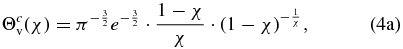
The spherical shell distribution of pick-up protons, PPUI(w; wPUI; Δw), can be approached by a rectangular function in the velocity space. (Note that with  , we denote the proton velocities in the reference frame of the bulk solar wind, while
  denotes the velocities in the frame of the heliosphere.) This is generally expressed as follows:
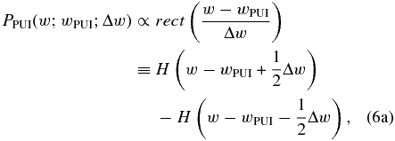
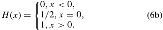
where H(x) is the Heaviside-step function,
After normalization, we have
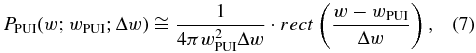
where the normalization constant is equal to the spherical shell volume, which is given by
The bulk solar wind protons are described by the three-dimensional kappa distribution (Livadiotis & McComas 2009). The κ-index that labels this distribution characterizes the stationary state of solar wind protons. Usually solar wind exists at more than one specific stationary state (at any heliocentric distance). In this paper we use quasi-equilibrium stationary states in order to describe the solar wind, prior to the incorporation of pickup ions; for kappa indices larger than κ ∼ 10, the kappa distribution is extremely close to a Maxwellian:

After the inclusion of pick-up protons, the solar wind flow includes two populations of protons, the solar wind protons described by the Maxwellian distribution PS(w; θ), and the pick-up protons described by the spherical shell distribution PPUI(w; wPUI; Δw). All the protons of the two populations are indistinguishable, equally sharing the newly formed hybrid state. The relevant hybrid probability distribution is written in terms of the hybridization fraction of pick-up protons χ, as follows:
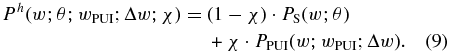
Inside the shell,  , the part of (1 − χ) · PS(w; θ) is quite small. Indeed, let us examine this for the representative case of w = wPUI. For aPUI ∼ 90° (e.g., for
  and φ ∼ 0°) we have
  . For
. For  km s−1 near Earth (∼1 AU) we have
  km s−1 near the termination shock (∼100 AU, near the nose; cf. Figure 1 in Whang et al.). Hence, for wPUI≅350 km s−1, kBT≅10 eV (T≅116, 000K or θ≅44 km s−1), and χ = 0.5, we find that (1 − χ) · PS(wPUI; θ)≅0.59 × 10−39, while the complementary part of χ · PPUI(wPUI; wPUI; Δw) is χ/(4πw2PUIΔw)≅0.93 × 10−9/ΔwRel, where ΔwRel ≡ Δw/wPUI. With almost 33 orders of magnitude smaller for a typical thickness of ΔwRel = 10−3, or 30 orders of magnitude smaller for the extreme case of maximum thickness ΔwRel = 1, the contribution of the original distribution (1 − χ) · PS(w; θ) inside the shell
  can surely be ignored. Hence,
In Figure 6 we depict the hybrid probability distribution (its logarithm), for various values of temperature, spherical shell radius, and thickness. Note that reasonable values of temperature for the heliospheric plasma are from T≅104 K (lower value for inner heliosphere) to T≅3 × 10⁶ K (upper value for inner heliosheath) that corresponds to values of θ from ∼13 km s−1 to ∼224 km s−1. In the examples demonstrated in Figure 6 we use θ = 200 km s−1 and θ = 150 km s−1.

Figure 6. Hybrid probability distribution of velocities (given in the bulk solar wind reference frame with  and
and  ) for two examples with temperature values, θ = 200 km s-1 (red) and θ = 150 km s-1 (blue). The thickness is taken to be Δw = 20 km s-1 and Δw = 40 km s-1, respectively. We consider three cases of spherical shell radius, (1) wPUI = 300 km s-1, (2) 400 km s-1, and (3) 500 km s-1.
Download figure:
Standard image High-resolution image4.2. Entropy and Transitions Further from Equilibrium
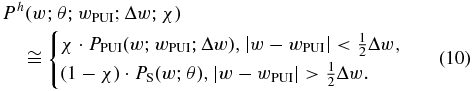
For stationary states close to equilibrium, entropy can be derived from its Boltzmann–Gibbs statistical formulation, namely,
where we indicate only the velocity dependence of probabilities for simplicity; Sh is the entropy of the hybrid state; the entropy units are given in terms of the Boltzmann constant kB; σ is a speed scale parameter, characteristic of the system and given by σ3 = VPUI or σ = θ (see similar treatment in: Tsallis et al. 1995; Prato & Tsallis 1999; Livadiotis & McComas 2010a). Note that we deal with the average entropy, i.e., entropy per particle. By substituting Ph(w), as given in Equation (10), into Equation (11), we conclude that the entropic variation ΔS between the entropy Sh of the hybrid state and the entropy S0 of the stationary state at equilibrium is given by (see Appendix B)

Equation (12) reads that pick-up protons will divert the system closer to equilibrium if Θd < 1, or further from equilibrium if Θd > 1. As soon as the fraction χ of the pick-up protons, the temperature, and bulk velocity of solar wind protons have suitable values so that Θd > 1, namely, the solar wind thermal fluctuations are stronger than the radial fluctuations of pick-up protons, then the average entropy decreases. This justifies the conjecture postulated in Livadiotis & McComas (2010a) that the pick-up ions can have an effective organizing role in space plasmas and decrease their (average) entropy.
5. DISCUSSION
Having developed the characteristic fluctuation number, Θd, and explained its physical meaning and connection to the change in average entropy ΔS of joint particle distributions, it is straightforward to find its values in the heliosphere. Combining Equations (3) and (4a) we have
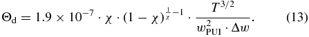
A typical value of the fluctuation number Θd in the inner heliosphere is ∼10−7, obtained for χ = 0.001,  , T = 104 K,
  (and δa = 5°), and φ = 0° (nose). This is a very small value and we hardly expect to find any position in the inner heliosphere where the pick-up protons significantly decrease the entropy of the solar wind protons. This holds even in some more distant locations in the heliosphere, e.g., near and sunward of the termination shock. The fluctuation number is simply increased by two orders of magnitude, Θd ∼ 10−5, for the parameter values χ = 0.01,
  , T = 5 × 10⁴ K,
  , δa = 5°, and φ = 0°. However, in the inner heliosheath the fluctuation number should be much larger, i.e., Θd ∼ 1 for χ = 0.3,
  , T = 3 × 10⁶ K, while Θd ∼ 10 for χ = 0.6,
  , T = 3 × 10⁶ K (see Table 1).
Table 1. Fluctuation Number and Entropy within the Heliosphere
| Location | T (K) |  |
χ | Θd | ΔS |
|---|---|---|---|---|---|
| Inner heliosphere | 104 | 20 | 0.001 | ∼10−7 | >0 |
| ≫ | 5 × 10⁴ | 15 | 0.01 | ∼10−5 | >0 |
| Inner heliosheath | 3 × 10⁶ | 10 | 0.3 | ∼1 | ∼0 |
| ≫ | 3 × 10⁶ | 5 | 0.6 | ∼10 | <0 |
| ≫ | 3 × 10⁶ | 5 | >0.9 | ∼20–30 | <0 |
Notes. The values are taken for φ = 0° (nose) and for pitch angle  and deviation δa = 5°. These do not have any important effect on the fluctuation number in the inner helioshere. In the inner heliosheath the fraction χ may take very large values such as χ ≈ 0.982 (nPUI ≈ 2.5 cm−3, nS ≈ 0.045 cm−3, e.g., cf. Figure 2 in Chalov et al. 2004).
Download table as: ASCIITypeset image
Since the fluctuation number Θd is typically small in the inner heliosphere, we examine its maximum values whether these can be larger than 1 or not. Therefore, we examine the maximum fluctuation number; the solar wind bulk velocity is  , while the thickness is minimized when the pitch angle is taken to be the approximately supplementary angle of the longitude,
  . In (13) we observe that for deriving the distribution of Θd in the heliosphere, we need the heliospheric values of several other parameters, such as the fraction χ, the solar wind bulk velocity
  , the temperature T, and the pitch angle
  (its deviation δa is a free parameter rather than depending on the heliospheric position). In order to express Θd as a function of heliocentric distance r, the expressions for T(r),
  and χ(r) are needed. T(r) and
  are taken from the fitting of data from Ulysses and Voyager 2 (cf. Figure 1 in Wang & Richardson 2001) compared also with the formulae given in Whang et al. (2003). χ(r) is taken from (Richardson & Stone 2009). These heliocentric functions are valid for longitudes near the nose, i.e., from φ≅0° to φ≅ ± 30°. We find that for any pitch angle
  and deviation δa, the fluctuation number Θd increases with heliocentric distance r, but becomes ∼1 far beyond the termination shock. Hence, concerning the observational data (for φ near the nose), we conclude that no decrease of the entropy can be caused by the organizing effect of the pick-up protons on the solar wind protons sunward of the termination shock. Furthermore, in Figure 7 we show the longitude dependence of Θd for χ = 0.5, temperature values T = 3 × 10⁴ K, 3 × 10⁵ K, 3 × 10⁶ K, and pitch angle deviation δa = 10°, 5°, 0°. Similarly, in Figure 8 we show the longitude dependence of Θd for χ = 0.3, and temperature values T = 2 × 10⁴ K, 2 × 10⁵ K, 2 × 10⁶ K.

Figure 7. Logarithm of the fluctuation number (by density), log Θd, depicted as a function of the longitude φ. The solar wind bulk velocity is  . The fraction is χ = 0.5, while the pitch angle is taken to be supplementary to the longitude, i.e.,
  . The panels in each column have different temperatures: T = 3 × 10⁴ K (left column), 3 × 10⁵ K (center column), 3 × 10⁶ K (right column), while in each row they have different pitch angle deviations, i.e., δa = 10° (upper row), 5° (middle row), and 0° (lower row). The critical value Θd = 1, for which the competing fluctuations are entropically equivalent, is indicated by the blue dashed horizontal line (at log Θd = 0). Values of Θd below the horizontal line correspond to ΔS > 0 (green), while above the horizontal line they correspond to ΔS < 0 (yellow). Note the slight asymmetry between ∼90° and ∼270°.
Download figure:
Standard image High-resolution image
Figure 8. Logarithm of the fluctuation number (by density), log Θd, depicted as a function of the longitude φ, similar to Figure 7. The fraction is χ = 0.3, while the values of temperature are T = 2 × 10⁴ K (left column), 2 × 10⁵ K (centered column), 2 × 10⁶ K (right column).
Download figure:
Standard image High-resolution imageIn Figures 7 and 8 we observe that for high temperature values up to T ∼ 106 K the logarithm of the fluctuation number is positive, log Θd > 0, leading to a decreasing average entropy, ΔS < 0. For lower temperatures (T ∼ 105 K and less), log Θd > 0 is achieved only for longitudes near ∼0° and ∼180°, and, if the pitch angle deviation δa is sufficiently small, near ∼90° and ∼270°. Solar wind protons with temperatures as high as T ∼ 106 K can be found only in the inner heliosheath. The temperature of the shocked ion distributions in the inner heliosheath was predicted by several models to be T ∼ 106 K on average (e.g., Heerikhuisen et al. 2008; cf. Figure 1 in Richardson & Stone 2009), and verified by the analysis of the IBEX-Hi spectra (Livadiotis et al. 2011).
It is interesting that while the plasma in the heliosphere sunward of the termination shock exhibits an increasing average entropy, ΔS > 0, the opposite holds beyond the termination shock in the inner heliosheath, where the pick-up protons are effectively organizing the solar wind protons exhibiting ΔS < 0. The pick-up protons interact with the solar wind protons and decrease the entropy of the coupled system, moving it into "far-equilibrium" stationary states. This statement was first postulated by Livadiotis & McComas (2010a), and verified by the IBEX observations as shown in the analysis of Livadiotis et al. (2011). Here we presented a solid analytical proof of this statement, which can also be used to find analytically the predicted velocity distributions after the entropy reduction.
Livadiotis & McComas (2010a) showed that a specific connection of the variance of the distribution with the temperature changes the entropic behavior depending on the κ-index in principle. By expressing the entropy in terms of the κ-index, S(κ), it was shown how variations of entropy can gradually lead the system toward, or away from, equilibrium. Entropy S(κ) is generally a non-monotonic function with respect to the κ-index. In particular, it is monotonic in the near-equilibrium region, i.e., for ∞ > κ > 2.5, while the non-monotonicity (concave upward) appears in the far-equilibrium region, i.e., for 2.5 ⩾ κ > 1.5, exhibiting thus a more complicated behavior.
In the near-equilibrium region, the entropy S(κ) increases with the κ-index,
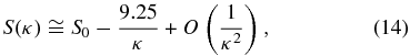
with  (B8). Therefore, starting at equilibrium, which corresponds to the maximum κ-index (κ → ∞) and a Maxwellian distribution, any decreases of entropy will lead to kappa distributions with smaller κ-indices, and thus, the system will be directed further from equilibrium. Hence, ΔS ≡ S(κ) − S0 = −9.25/κ, and when ΔS < 0, this gives a solution for a finite κ-index. The initial Maxwellian distribution is replaced by a kappa distribution of (finite) κ-index given by

Starting from a quasi-equilibrium stationary state that corresponds to a large κ-index in the near-equilibrium region (κ ≫ 2.5), the entropy variation between two stationary states with κ-indices κ1 → κ2 is given by

Therefore, if the entropy of the system varies by ΔS, then its initial kappa distribution of index κ1 will be replaced by a kappa distribution of index κ2, given by
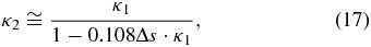
and thus, the system will transmit in a stationary state with κ2 nearer to equilibrium (for ΔS > 0), or further from equilibrium (for ΔS < 0). The relation between the initial κ1 and the resulting κ2 κ-indices is shown in Figure 9 for various values of the entropy variation, either positive ΔS > 0 (green) or negative ΔS < 0 (yellow). The red arrow indicates an example for ΔS≅ − 0.7, where the initial kappa distribution of κ1≅40 after the entropy reduction leads to a resulting kappa distribution of κ2≅10. The blue arrow shows the opposite case of increasing entropy ΔS≅0.7, where the initial kappa distribution of κ1≅10 leads to a resulting kappa distribution of κ2≅40.

Figure 9. Non-equilibrium transitions caused by entropy variations. If the entropy of a system varies by ΔS, then its initial kappa distribution of index κ1 will go to a kappa distribution of index κ2, as given by Equation (17), which is valid for sufficiently large κ-indices (κ ≫ 2.5). Then, the system transits in a stationary state with κ2 nearer (for ΔS > 0) or further from equilibrium (for ΔS < 0). In the case of the solar wind protons described initially by a kappa distribution of κ1, pick-up ions in the inner heliosheath can effectively reduce the system's entropy leading to incorporated solar wind protons described by a kappa distribution of κ2 < κ1 (further from equilibrium). On the contrary, pick-up ions increase the system's entropy in the heliosphere sunward of the termination shock, resulting in a kappa distribution of κ2 > κ1 (nearer to equilibrium). An example of decreasing entropy is shown by the red arrow where the initial index κ1≅40 leads to an index κ2≅10 for ΔS = −0.7 (for even larger entropy decreases, we have even smaller κ-indices, i.e., κ2≅5 for ΔS = −1.5, and κ2≅3 for ΔS = −3). The blue arrow shows the opposite case of increasing entropy, where the index κ1≅10 leads to κ2≅40 for ΔS = 0.7.
Download figure:
Standard image High-resolution imageFinally, we note that there are a variety of other processes that may become important beyond the termination shock with the shock heating and scattering both the solar wind and pick-up ions. The present work has been restricted to the large-scale topological properties of the interplanetary magnetic field, and in the specific ways that these properties can be involved in the pick-up ion distributions, e.g., via the pitch angle (its average value and deviation). In this way, we explicitly excluded small-scale magnetic variations and structures, e.g., turbulent magnetic fields, which, however, do affect the detailed particle distributions. Furthermore, it is very interesting that in spite of various global models of the heliosphere that were based on the assumption that the magnetic field in the heliosheath would be laminar, recent analyses show that the magnetic field in the heliosheath may in fact not be laminar at all and may even consist of magnetic bubbles (e.g., Drake et al. 2006; Opher et al. 2011). Folding of the heliospheric current sheet in the heliosheath could be another important factor in determining the solar wind dynamics therein. Nonetheless, our analysis here focuses on the interaction and evolution of the solar wind and pick-up ion populations, with emphasis on the role of pick-up ions in modifying the entropy of the solar wind plasma.
6. CONCLUSIONS
In this paper we showed how the addition and incorporation of highly ordered distributions of pick-up ions can increase the ordering of space plasmas decreasing its entropy, and driving it away from equilibrium. We presented a model for describing the entropy decrease in space plasma protons, potentially caused by the pick-up protons and their highly ordered arrangement. The flow of protons consists of two populations, the solar wind protons that are in stationary states close to thermal equilibrium and well described by a Maxwellian distribution, and the pick-up protons described by a spherical shell distribution.
The solar wind protons are described by kappa distributions. These distributions characterize stationary states out of equilibrium, with their kappa index, κ, providing a measure of how far the stationary state is from equilibrium (Livadiotis & McComas 2010a, 2010b, 2010c). The model presented was used for quasi-equilibrium stationary states in order to describe the solar wind, prior to incorporation of pick-up ions; for κ-indices larger than κ ∼ 10, the kappa distribution is extremely close to a Maxwellian distribution.
The variation in the average entropy (entropy per particle) between the hybrid state (after the entrance of pick-up protons) and the original stationary state of the bulk solar wind protons, ΔS, depends on a dimensionless "fluctuation number," which is a measure of the organizing role of the pick-up protons in the solar wind flow. This number characterizes and compares the two competing fluctuations of the thermal motion of the solar wind protons, and of the bounded motion of the pick-up protons that forms the spherical shell distribution. We derived two different but relevant definitions of this fluctuation number; the fluctuation by volume, ΘV, and fluctuation by density, Θd. The former, ΘV, is simply the ratio of the characteristic cubic volume VS of the thermal fluctuations of bulk solar wind protons, with the volume in which the pick-up protons are fluctuated, that is, their spherical shell volume, VPUI. The latter, Θd, is proportional to the ratio of the phase space density of the pick-up protons with the relevant density of the bulk solar wind protons. These are the phase space densities corresponding to the relevant fluctuation volumes VPUI and VS. The fluctuation by volume definition is expressed in terms of the temperature and bulk velocity of the solar wind protons, as well as the thickness of the pick-up proton spherical shell. The fluctuation by density Θd, is actually equal to, ΘV multiplied by a specific function of the fraction χ of the pick-up protons in the solar wind. This was conveniently set so that the value Θd = 1 corresponds to no change in entropy. Therefore, when Θd > 1 we have strong thermal fluctuations of the bulk solar wind protons, and the entrance of the less disorganized pick-up protons decreases the entropy, i.e., ΔS < 0. When Θd < 1, then the bulk solar wind protons are already well organized and the entrance of the more disorganized pick-up protons increases the entropy, i.e., ΔS > 0. In the critical case of Θd = 1, the two competing fluctuations somehow balance each other, causing no change to the entropy, i.e., ΔS = 0. This is consistent with the proportionality of ΔS to the negative logarithm of Θd, ΔS∝ − ln Θd.
This relation was analytically demonstrated by considering that all the protons are indistinguishable, equally sharing a hybrid state. Therefore, the solar wind protons together with the pick-up protons are characterized by a probability distribution that is the normalized sum of the probability distributions of the bulk protons (kappa distribution) and the pick-up protons (spherical shell distribution). Potentially, this hybrid describes a more organized state, having lower entropy than the stationary state assigned by the original probability distribution of the solar wind before the inclusion of pick-up protons.
We calculated the possible values of Θd in the heliosphere and the consequences on the entropy and the transitions of solar wind as a thermodynamical system. While sunward of the termination shock the entropy generally increases, beyond the termination shock in the inner heliosphere, where the pick-up ions can be found in large fractions, the entropy decreases significantly. The decrease of entropy redirects the proton population back to far-equilibrium. Therefore, the model concludes that the heliosphere sunward of the termination shock resides mostly in near equilibrium stationary states, while the inner heliosheath resides mostly in far equilibrium stationary states. The latter was verified by the recent analysis on IBEX-Hi ENA spectra (Livadiotis et al. 2011). Other, more distant, astrophysical systems have vastly different plasma parameter regimes, where the effects of both strongly enhancing entropy (driving the system toward equilibrium) and strongly decreasing entropy (driving the system toward more order and away from equilibrium) may have critical implications for the evolution of plasma environments and remotely observable emissions. For instance, Soker et al. (2010) showed that the presence of pick-up ions in some planetary nebulae and symbiotic astrophysical systems might reduce the post-shock temperature of the fast wind and jets. These pick-up ions might also reduce the entropy of these systems, leading them into far-equilibrium transitions.
Livadiotis & McComas (2010a) showed that spontaneous increases in entropy gradually lead the system toward equilibrium. On the contrary, any exterior factor that decreases the entropy can redirect the plasma back to far from equilibrium stationary states. Here we examined the specific mechanism of decreasing entropy that is related to the pick-up ions as soon as they can add "order" to the solar wind protons. Indeed, at least in the inner heliosheath, their highly ordered arrangement, which arises in the small thickness of their spherical shell distribution, decreases the average entropy and redirects the system away from equilibrium.

Figure 10. Pick-up proton (p+) velocity in the solar wind (SW) flow reference frame. The dotted and dashed arrows show the solar wind (SW) and LISM flows, respectively. The angles ϑ, β, a, ϕ and the longitude from the nose φ = 180° − ϕ, are indicated, as defined in the text. In (a) we show the LISM flow that vertically hits the solar wind flow (φ = 90°), while in (b) the LISM hits the solar wind at an arbitrary longitude φ. Here we demonstrate the case of a = 90°, i.e., the interplanetary magnetic field  is vertical to the solar wind flow.
Download figure:
Standard image High-resolution image
APPENDIX A: THICKNESS OF THE SPHERICAL SHELL DISTRIBUTION OF PICK-UP PROTONS
A.1. Pitch Angle of Pick-up Protons Equal to aPUI = 90°
We begin our approach for estimating the thickness, Δw, by setting the pitch angle of pick-up protons aPUI ≡ a + ϑ equal to 90°, i.e., considering the simple example where the pick-up proton velocity  is perpendicular to the interplanetary magnetic field
  . In this case, Equation (1) gives
  . First we examine the case where the LISM flow is perpendicular to the solar wind flow, i.e., ϕ = 90° (perpendicular to the heliospheric nose–tail direction) (Figure 10(a)), and subsequently we examine the general case of the arbitrary direction of solar wind flow (arbitrary angle ϕ between the LISM and solar wind flow) (Figure 10(b)). The angle ϕ is supplementary to the longitude from the nose, φ, i.e., φ = 180° − ϕ.
A.1.1. Longitude φ = 90°
The radius  of the spherical shell is
  (Figure 10(a)). This is because the pick-up proton is created with an initial velocity approximately equal to the parent neutral hydrogen atom velocity, namely, ∼
 (in the heliosphere reference frame). However, any possible loss of energy during its creation leads to a smaller initial velocity that can typically vary from 0 to ∼
 , and thus, the spherical shell radius varies in the interval
  (triangle in Figure 10(a)). Consequently, an estimation of the thickness of the shell Δw can be given by the difference between the maximum and the minimum value of the spherical radius, i.e.,
  , or
, or

where  . Given that
  or εL≅4.12 eV (e.g., cf. Table 2 in Frisch et al. 2002), we find

where both velocities,  and Δw, are expressed in km s−1.
For example, we consider the distant solar wind in the outer heliosphere near the termination shock (that is, at a heliocentric distance of ∼100 AU near the nose) with a bulk velocity of about  (this corresponds to a bulk velocity of about
  near Earth (∼1AU); e.g., cf. Figure 1 in Whang et al. 2003). Hence, we have wPUI≅350 km s−1, or in terms of (kinetic) energy, εS≅640 eV (for protons). Then, the thickness is Δw≅1.13 km s−1 or εΔw≅0.00663 eV, while its ratio to the whole radius is
  . Finally, the volume of the spherical shell is VPUI = 1.73 × 10⁶ (km s−1)3.
A.1.2. Arbitrary Longitude φ
The spherical shell radius wPUI varies in the interval  (triangle in Figure 10(b)). Now the shell thickness is

A.2. Arbitrary Pitch Angle of Pick-up Protons aPUI
We proceed by calculating the thickness for any arbitrary values of a, and ϑ. The spherical shell radius is given by (1), i.e.,  , and by varying the three included quantities,
  , a, and ϑ, we find the total variation of wPUI, that is δwPUI. Indeed,

where  , δa, and
  , δϑ are the expectation values and deviations of the angles a and ϑ, respectively. For a given longitude φ, the small angle ϑ varies from 0 to a maximum value ϑMax given by

so its average value and deviation are estimated by half of this maximum value

The radius wPUI varies from wPUI − δwPUI to wPUI + δwPUI, thus, the spherical shell thickness is given by Δw = 2 · δwPUI. Hence, we have

where the variation  equals the thickness that was estimated for the case aPUI = 90° (given in Equation (A3)). Thus,

Hence, we find

with  and
and

We stress the fact that the shell thickness Δw(φ; aPUI = 90°) (A3) is due to mechanical and not geometrical or statistical factors; namely, the initial pick-up proton velocity can vary from 0 to  because of loss of energy. Further, Equation (A4) also includes the statistical variations of the angles a and ϑ. Finally, it will be interesting to include thermal variations of the bulk velocities
  and
and  in the thickness formulation. In addition, we note that a more accurate approach would include both the heliospheric longitude φ and latitude θ. In this case the angle ϕ has to be replaced by cos ϕ = −cos φ · cos θ.
APPENDIX B: ENTROPY VARIATION CAUSED BY PICK-UP IONS
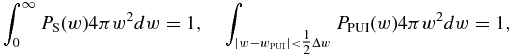
In this appendix we prove the formula given in Equation (12), ΔS = −kB · χ · ln Θd. According to the Boltzmann–Gibbs statistical formulation, the entropy Sh of the hybrid probability distribution Ph(w) is given by Equation (11):

where σ is a speed scale parameter, characteristic of the system. A reasonable value for this can be given by σ3 = VPUI or σ = θ (Livadiotis & McComas 2010b). However, we mention that, in the end, the value of σ is not important because it is eventually cancelled out. Then, substituting Ph(w) from Equation (10) into Equation (B1) yields

which is
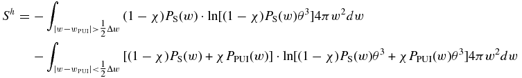

with

We approximate the integrand G(w; x) following the step from Equations (9) to (10) in Section 4

Hence,

Ultimately, Equation (B1) gives
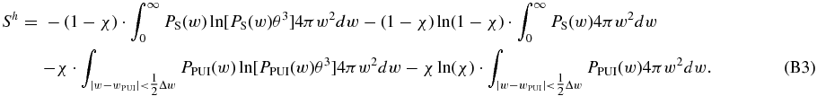
By utilizing the normalizations
and the entropy at equilibrium, S0

the hybrid entropy in Equation (B2) becomes

Then, substituting the fluctuation number by volume Θv = θ3/VPUI into Equation (B4) yields

and thus, the entropy variation is given by

where we substituted S0 defined in Equation (B4) which equals

Hence, Equation (B7) is written as

where Θcv(χ) is given by Equation (4a) so that ΔS = 0 when Θv = Θvc. Finally, using Equation (5) and restoring the Boltzmann's constant kB yields
