


ABSTRACT
The γ-ray sky >100 MeV is dominated by the diffuse emissions from interactions of cosmic rays with the interstellar gas and radiation fields of the Milky Way. Observations of these diffuse emissions provide a tool to study cosmic-ray origin and propagation, and the interstellar medium. We present measurements from the first 21 months of the Fermi Large Area Telescope (Fermi-LAT) mission and compare with models of the diffuse γ-ray emission generated using the GALPROP code. The models are fitted to cosmic-ray data and incorporate astrophysical input for the distribution of cosmic-ray sources, interstellar gas, and radiation fields. To assess uncertainties associated with the astrophysical input, a grid of models is created by varying within observational limits the distribution of cosmic-ray sources, the size of the cosmic-ray confinement volume (halo), and the distribution of interstellar gas. An all-sky maximum-likelihood fit is used to determine the XCO factor, the ratio between integrated CO-line intensity and H2 column density, the fluxes and spectra of the γ-ray point sources from the first Fermi-LAT catalog, and the intensity and spectrum of the isotropic background including residual cosmic rays that were misclassified as γ-rays, all of which have some dependency on the assumed diffuse emission model. The models are compared on the basis of their maximum-likelihood ratios as well as spectra, longitude, and latitude profiles. We also provide residual maps for the data following subtraction of the diffuse emission models. The models are consistent with the data at high and intermediate latitudes but underpredict the data in the inner Galaxy for energies above a few GeV. Possible explanations for this discrepancy are discussed, including the contribution by undetected point-source populations and spectral variations of cosmic rays throughout the Galaxy. In the outer Galaxy, we find that the data prefer models with a flatter distribution of cosmic-ray sources, a larger cosmic-ray halo, or greater gas density than is usually assumed. Our results in the outer Galaxy are consistent with other Fermi-LAT studies of this region that used different analysis methods than employed in this paper.
Export citation and abstract BibTeX RIS
1. INTRODUCTION
The diffuse Galactic γ-ray emission (DGE) is produced by cosmic-ray (CR) particles interacting with the gas and radiation fields in the interstellar medium (ISM). As has been recognized since the late 1950s (Morrison 1958), measurements of the DGE can be used to study CR origin and propagation in the Galaxy, and also to probe the content of the ISM itself, independent of other methods. They are complementary to direct measurements of CRs by balloons and satellites, and to radio astronomical surveys of synchrotron radiation that is produced by CR electrons and positrons losing energy in the Galactic magnetic field.
The first γ-ray observations made by the OSO-3 satellite (Kraushaar et al. 1972) showed emission in the inner Galaxy. The breakthrough came with the SAS-2 (Fichtel et al. 1975) and COS-B (Bignami et al. 1975a) instruments, whose Galactic plane surveys above 100 MeV allowed testing of DGE models based on CRs and their interactions in the ISM (e.g., Puget & Stecker 1974; Bignami et al. 1975b; Stecker et al. 1975; Bloemen et al. 1986; Strong et al. 1988). The COMPTEL and EGRET instruments on the Compton Gamma-Ray Observatory provided higher-quality data covering the entire sky in the energy range 1 MeV–10 GeV, which stimulated more detailed modeling (Hunter et al. 1997; Strong et al. 2000, 2004b, 2004c). Recently, the SPI instrument on the INTErnational Gamma-Ray Astrophysics Laboratory (INTEGRAL) observatory has extended the observations of CR-induced diffuse emissions into the hard X-ray range (Bouchet et al. 2008, 2011), while ground-based instruments (Aharonian et al. 2006; Abdo et al. 2008) have detected emission at TeV energies from the Galactic plane and Galactic center regions that are likely to have a CR-induced origin. For a recent pre-Fermi review of the subject see Strong et al. (2007).
The Fermi Large Area Telescope (Fermi-LAT) provides a view of the entire γ-ray sky from 30 MeV to beyond several hundred GeV with a sensitivity surpassing its predecessor instrument, EGRET, by more than an order of magnitude. Studies of the DGE by the Fermi-LAT Collaboration have so far concentrated on specific regions of the sky. At intermediate Galactic latitudes, Fermi-LAT observations did not confirm the EGRET "GeV excess" and showed that the spectrum was consistent with a DGE model based on measured CR spectra (Abdo et al. 2009a). The emissivity of nearby H i gas was derived from analysis of a selected high-latitude region (Abdo et al. 2009b) and found to agree with the emissivity calculated assuming measured CR spectra. Analysis of data for the second and third Galactic quadrants (Abdo et al. 2010d; Ackermann et al. 2011b) showed a higher-than-expected H i emissivity in the outer Galaxy with respect to the DGE model used by Abdo et al. (2009b). These studies of the outer Galaxy also indicated a lower XCO factor (the ratio between integrated CO-line intensity and H2 column density) compared to that used by Strong et al. (2004a). The early studies with the Fermi-LAT data have systematically moved from understanding the DGE produced by CRs interacting with the relatively nearby ISM to progressively larger regions of the Galaxy.
Modeling the DGE requires knowledge of CR intensities and spectra, along with the distributions of interstellar gas and radiation fields, throughout the Galaxy. Starting from the distribution of CR sources and the injection spectra of CRs, the CR intensities and spectra can be estimated by modeling their propagation in the Galaxy, taking into account relevant energy losses and gains. The resulting CR distributions are then folded with the target distributions of the interstellar gas and radiation fields to calculate the DGE (e.g., Strong et al. 2004c). Defining the input distributions and calculating the models is not a trivial task and involves analysis of data from a broad range of astronomical and astroparticle observatories.
CR propagation models can be constrained to a certain extent using measurements of CRs in the solar system (see, e.g., Strong et al. 2007 for a recent review). For an assumed propagation model, e.g., plain diffusion, diffusive-reacceleration, diffusion-convection, etc., the propagation parameters of the model and size of the CR confinement region can be derived by comparing the modeled secondary-to-primary CR nuclei ratios with data. However, some key components are difficult to constrain with this method. An example is the CR source distribution because the CR data essentially probe only relatively nearby sources, and not the Galaxy-wide distribution. Because γ-rays are undeflected by magnetic fields and absorption in the ISM is negligible below ∼10 TeV (Moskalenko et al. 2006b), the DGE is a direct probe of the CR intensities and spectra in distant locations, allowing the study of the Galactic distribution of CR sources.
In this paper, we analyze the DGE from the full sky observed with Fermi-LAT. We use data from the first 21 months of observations with Fermi-LAT for energies 200 MeV–100 GeV that contain the lowest fraction of background events in the Fermi-LAT data. The DGE is modeled using the GALPROP code (see, e.g., Moskalenko & Strong 1998; Strong et al. 2000, 2004b; Ptuskin et al. 2006; Porter et al. 2008; Vladimirov et al. 2011a, and references therein). We create a grid of DGE models by varying the CR source distribution, the CR halo size, and the distribution of interstellar gas. The models are constrained to reproduce directly measured CR data, and then compared to the γ-ray data using an iterative maximum-likelihood fitting procedure. Our fits allow for variations in the XCO factor, the fluxes and spectra of the point sources in the first Fermi-LAT catalog (1FGL; Abdo et al. 2010a), the intensity and spectrum of an isotropic γ-ray background component, and scaling of the optical and infrared component of the interstellar radiation field (ISRF). We compare the likelihood of the models, and match observed and predicted intensities and spectra for various regions of the sky. Maps of the residual γ-ray emissions after subtraction of the DGE models are presented with the discussion of possible interpretations.
Our study is necessarily limited due to the (potentially) large number of DGE model parameters. Only diffusive-reacceleration models are considered for the CR propagation, even though models with convection and even plain diffusion models can in some cases provide an equivalent fit to the CR data (Strong et al. 2007). We assume a smooth distribution of CR sources with homogeneous injection spectra, although we expect CRs to originate in discrete sources and show variability in their emission spectra (Abdo et al. 2010b, 2010c, 2010e, 2010f). Because the homogeneity assumption tends to mainly affect the CR electrons, this is a very good approximation for the source distributions of the CR nuclei producing the bulk of the DGE in the energy range considered in this paper. Our propagation and emissivity calculations are limited to two dimensions (2D). Depending on the correlation of CR sources and gas densities, three-dimensional (3D) calculations taking the spiral arm structure of the Galaxy into account might quantitatively change the results of the paper even though the azimuthal-averaged distributions are not changed. Our qualitative conclusions are, however, independent of these assumptions.
The intent of this paper is not to find the perfect DGE model, but rather to test a selection of astrophysically motivated models and their compatibility with γ-ray observations. An essential aspect of this study is also assessing the impact of uncertainties involved in the many astrophysical inputs needed for a proper calculation of the DGE. Finally, we compare our results with the earlier mentioned analyses by the Fermi-LAT Collaboration that have used different methods to this paper.
2. DATA PREPARATION
The Fermi-LAT instrument, event reconstruction, and response are described by Atwood et al. (2009). In this paper, we use the Pass 6 DataClean event selection and instrument response functions (IRFs) employed in Abdo et al. (2010g) to derive the isotropic γ-ray intensity and spectrum. The DataClean event selection is used for our analysis because of the greatly reduced CR background, particularly in the 10–100 GeV energy range, compared to the standard low-background Diffuse class event selection (Atwood et al. 2009). The slight reduction in effective area compared to the Diffuse class IRFs is not a limitation for this analysis because the data are not limited by counting statistics for energies <100 GeV. The reduced CR background is especially important at high latitudes where the γ-ray signal is weakest. For the description of the procedure to select these data and generate the IRFs, we refer to Abdo et al. (2010g). Note that we restrict the upper energy range of our analysis to 100 GeV because the CR background for the DataClean event selection is determined only up to this energy.
We use 21 months of data, starting from 2008 August 5 to 2010 May 4. To minimize the contribution from the very bright Earth limb, we apply a maximum zenith angle cut of 100°. In addition, we also limit our data set to include only photons with an incidence angle from the instrument z-axis of <65°. The rejection power for CRs is reduced at large incident angles and the fraction of events converting in the thick tracker layers increases, causing the effective point-spread function (PSF) to worsen significantly (Atwood et al. 2009). The signal loss is minimal because the effective area for γ-rays is reduced significantly at high-incidence angles. Exposure maps and the PSF for the pointing history of the observations were generated using the standard Fermi-LAT ScienceTools package available from the Fermi Science Support Center.58 We use the GaRDiAn package (see Appendix A for a description) to process the data and exposure maps to produce all-sky intensity maps, and the same package for the maximum-likelihood fitting procedure. The counts are spatially binned with a HEALPix59 order 7 isopixelization scheme giving an angular resolution ≈0 5 (Górski et al. 2005). For the fitting procedure, the data are binned with nine equally spaced logarithmic bins between 200 MeV and 100 GeV. This relatively coarse energy binning is used to ensure stable fits for the point sources that have a free scaling parameter for each energy bin. The intensity maps are created by dividing the counts map with the exposure that is weighted using a DGE model. The model weighting of the exposure is required because of the strong energy dependence of the exposure at energies below ∼1 GeV (Abdo et al. 2010g). However, this causes insignificant variations between the intensities for the different DGE models considered in this paper due to the similarity of their spectra. Note that for our plots of the intensities for the DGE models and data, we use 15 equally spaced logarithmic energy bins for the same energy range to better utilize the energy resolution of the Fermi-LAT instrument.
When comparing the data and models we perform the maximum-likelihood fit in photon space, forward folding the models to create the expected counts, using the exposure maps and PSF as described in Appendix A. To ensure that we properly take the PSF into account for the spectra and longitude/latitude profiles, we calculate the model intensity maps from their expected counts in the same way as the intensity maps of the observed counts. This ensures that the comparison of intensity and photon counts is consistent. When selecting special regions of the sky, all pixels whose centers are within the region are used. Because the pixel size is significantly smaller than these regions the edge effects are minimal.
The systematic error in the effective area of Fermi-LAT is estimated to be 10% below 100 MeV, 5% at 562 MeV, and 20% above 10 GeV with linear interpolation in logarithm of energy between the values (Abdo et al. 2010g). The systematic error is not taken into account in the parameter estimates but is included in the figures below, which compare the spectra and profiles of the models to the data.
The selection corresponding to the Pass 760 data used for the second Fermi-LAT source catalog (2FGL; Nolan et al. 2011) was not available at the start of the analysis presented in this paper. The effect of the improved IRFs in the several-GeV energy range was tested by repeating the last step of the analysis for a single model using the Pass 7 clean photon class. The data were prepared in the same way as the Pass 6 DataClean photons described above. The results of the test are described in Section 4.2.2.
3. GRID SETUP AND ANALYSIS PROCEDURE
We use a "conventional" CR propagation model paradigm where a set of CR propagation models that reproduce locally measured CR intensities and spectras is created. All of the models investigated in this paper are based on, and constrained by, a variety of non-γ-ray data: CRs measured near the Earth, the distribution of potential CR sources in the Galaxy derived from observations, and the distributions of interstellar gas and radiation fields from survey data and modeling. We summarize these details below.
3.1. Models of the Diffuse Galactic γ-Ray Emission
We use the recently released version 54 (ver. 54) of the GALPROP code (Vladimirov et al. 2011a) to create models of the DGE. We limit ourselves to models using diffusive-reacceleration with no convection for a Kolmogorov spectrum of interstellar turbulence as has been successfully used to explain CR data and the EGRET γ-ray sky (Strong et al. 2004b) as well as INTEGRAL data (Porter et al. 2008). For a detailed description of the GALPROP code and the improvements in ver. 54 with respect to earlier versions we refer the reader to the dedicated Web site.61
The parameter files of the GALPROP models used in this paper are available in the supplementary material to this paper available in the online journal. These give a precise definition of the models used which can be reproduced as required. Note that only one scaling factor for the ISRF is given in each file which is the average of the local and inner scaling factors found from the fit (see Sections 3.4 and 3.5.3).
The collection of models used in this analysis is created using the CR source distributions and propagation parameters as described in Section 3.2 for different sizes for the CR confinement region: for an assumed cylindrical geometry where the Sun is located in the Galactic plane 8.5 kpc from the Galactic center, we use radial boundaries, Rh, of 20 kpc and 30 kpc, and vertical boundaries (halo size), zh, of 4, 6, 8, and 10 kpc, respectively. In addition, we use two assumptions for the optical depth correction of the H i component (see Section 3.3.1) and also two values for the cut at which dust emission is no longer used to correct the total column density (see Section 3.3.4). This results in a total of 128 models.
3.2. Cosmic-Ray Injection and Propagation
Supernova remnants (SNRs) are believed to be the principal sources of CRs. However, their Galactic distribution is not well determined (Case & Bhattacharya 1998; Green 2005). Therefore we consider, in addition to the measured SNR distribution from Case & Bhattacharya (1998)62 (hereafter SNR distribution), other tracers of supernovae (SNe) explosions. The pulsar distribution is a prime candidate as a proxy distribution, because pulsars are an SN explosion end state. The distribution of pulsars is also better determined than SNRs. Still, it suffers from observational biases and for that reason we test two different pulsar distributions, one from Yusifov & Küçük (2004, hereafter Yusifov distribution) and another from Lorimer et al. (2006, hereafter Lorimer distribution). One of the main differences between the two distributions is the functional form used to fit the observational points. Both have a maximum between R = 0 and R = R☉ and fall off exponentially in the outer Galaxy. However, Lorimer et al. (2006) force the source spatial distribution to zero at R = 0, whereas it is non-zero in Yusifov & Küçük (2004). As an additional proxy for the distribution of CR sources, we consider the distribution of OB stars from Bronfman et al. (2000, hereafter OB stars distribution). OB associations are putative CR acceleration regions and these stars are also the progenitors of core collapse SNe that can leave compact objects, such as pulsars. The four CR source distributions used in this paper are plotted in Figure 1.

Figure 1. CR source density at z = 0 in arbitrary units as a function of Galactocentric radius. Solid black curve: SNRs (Case & Bhattacharya 1998). Dashed blue curve: pulsars (Lorimer et al. 2006). Dotted red curve: pulsars (Yusifov & Küçük 2004). Dash-dotted green curve: OB stars (Bronfman et al. 2000). While the units are arbitrary, the relative normalizations of the curves in the figure match those found in the GALPROP models used in this analysis. The CR flux of the models is normalized to the observed CR flux at the solar circle after propagation. The normalization is done at 100 GeV and is therefore unaffected by modulation.
Download figure:
Standard image High-resolution imageTo determine the CR injection spectra and propagation parameters we perform a χ2 fit to CR nuclei, electron, and positron data, using the Minuit263 minimizer. To reduce computation time, the fit is done in two parts. The propagation parameters and CR nuclei injection spectrum are found from a fit to the CR nuclei data first. The electron injection spectrum is then found by fitting to the total CR electron and positron spectrum, including the contribution by secondary electrons and positrons from CR protons and He interacting with the interstellar gas. Fitting the propagation parameters in the first step decreases the computation time because nuclei up to 14Si must be included in the propagation calculation for an accurate B/C ratio determination, while for the secondary electrons and positrons only protons and He are important. Not calculating the secondary electrons and positrons in the fit to the propagation parameters also saves a considerable amount of time. We use the CR database created by Strong & Moskalenko (2009) and use the data sets and parameters as discussed below. When comparing the models to the CR data we account for solar modulation using the force-field approximation (Gleeson & Axford 1968). In addition to the propagation parameters, the modulation potential for each experiment that has data below a few GeV (AMS, BESS, and ACE) is a free parameter during the fit. For Fermi-LAT and HEAO-3 we fixed the modulation at 300 MeV and 600 MeV, respectively, appropriate for the low solar activity during observations by each instrument as observed with the ACE satellite (Wiedenbeck et al. 2005). Solar modulation is unimportant for JACEE data.
3.2.1. Protons and Heavier Nuclei
We assume that the injection spectra for all CR nuclei species are described by the same rigidity-dependent function

where the indices and break rigidities are obtained by tuning the model to the observed spectrum of CR protons as well as the He, C, and O nuclei spectra. The low-energy intensity and spectrum are affected by solar modulation so we use data taken at low periods in the solar activity cycle. The inclusion of nuclei up to O is to ensure the major contributor species to the production of the secondaries B and Be are properly included. For the proton and He spectra we use low-energy data from BESS (Sanuki et al. 2000) and high-energy data from JACEE (Asakimori et al. 1998). For the C and O spectra we use low-energy data from ACE (ACE Team 2005) and high-energy data from HEAO-3 (Engelmann et al. 1990). To determine the diffusion coefficient, D0, and Alfvén speed, vA, for an assumed halo size, we use the B/C ratio because it is the most accurately observed secondary-to-primary ratio. Low-energy ACE (Davis et al. 2000) and high-energy HEAO-3 (Engelmann et al. 1990) data are used for this ratio.
The break in the CR proton and He spectrum observed by ATIC-2, CREAM, and PAMELA (Wefel et al. 2008; Ahn et al. 2010; Yoon et al. 2011; Adriani et al. 2011b) is not taken into account in this modeling and neither are the different spectral indices for protons and He. Vladimirov et al. (2011b) explore different scenarios for the break and different indices and find that the γ-ray intensities and spectra for their models are smaller than the systematic uncertainty of the Fermi-LAT effective area.
Because we derive constraints on the halo size from the γ-ray data, the radioactive secondary ratios are not directly used to fix the propagation conditions, as is usually the case in propagation model studies. However, the models are compared to the 10Be/9Be ratio to check the consistency of the constraints derived from the γ-rays. The 10Be/9Be data uncertainties are large enough to allow a halo size range from 4 kpc to 10 kpc (Strong et al. 2007), depending on the assumed propagation model. We keep the source abundances of nuclei fixed to values determined for ACE data (Moskalenko et al. 2008).
3.2.2. Electrons and Positrons
We assume the injection spectrum of primary CR electrons is described by the rigidity-dependent function

and use data from AMS (Aguilar et al. 2002), Fermi-LAT (Abdo et al. 2009c; Ackermann et al. 2010) and H.E.S.S. (Aharonian et al. 2008, 2009) to determine the spectral indices and break rigidities.64 Unfortunately, the data are insufficient to constrain the entire parameter set and unphysical values are obtained if all are freely fit. We therefore fix the values of γe, 1 = 1.6 and γe, 3 = 4, allowing only for freedom in ρe, 1, ρe, 2, and γe, 2. The γe, 1 used in this paper is consistent with that employed by Strong et al. (2011) for modeling the Galactic synchrotron emission, while the exact value of the high-energy index does not significantly affect our results. There is a strong correlation between γe, 1 and the modulation potential for the AMS data in the fits. We therefore caution that the derived values for the modulation potential are biased, although they are in reasonable agreement with the values derived by ACE for the same period (Wiedenbeck et al. 2005). The primary electron injection spectrum is dependent on that obtained from the CR nuclei fits through the size of the confinement volume and corresponding propagation parameters, as well as the contribution of secondary CR electrons and positrons produced by the CR nuclei interacting with the interstellar gas.
The overall fit is made to the data as described above. The normalization is essentially determined from the Fermi-LAT total electron and positron data. No attempt is made to fit the increasing positron fraction reported by Adriani et al. (2009). These can be neglected because the contribution from the excess positrons at high energies to the γ-ray emission is small.
3.3. Interstellar Gas and its Tracers
The DGE in the energy range considered in this paper has a strong contribution from π0-decay emission.65 The treatment in GALPROP is described in detail by Moskalenko & Strong (1998). For proton–proton interactions we use the formulation described in Kamae et al. (2006) for the calculation of the production cross sections. The production of pions from interactions of He nuclei with the interstellar hydrogen, as well as from collisions of CRs with interstellar He, are explicitly included, where we assume in this paper an interstellar He/H ratio of 0.11 by number (Strong & Moskalenko 1998). This is slightly higher than the canonical value of 0.1 found by observations of H ii regions (Deharveng et al. 2000), but it is within systematic uncertainty of those observations. We also ignore production of pions from CR and interstellar gas nuclei heavier than He while their contribution could be as high as ∼10% (Mori 2009). It is assumed that the distribution of interstellar He follows that of interstellar hydrogen, detailed below.
3.3.1. Atomic Hydrogen
The atomic hydrogen (H i) is the most massive component of the ISM and has a large filling factor, being observed in all directions. A recent comprehensive review of the H i content of the Galaxy can be found in Kalberla & Kerp (2009). For the CR propagation, the GALPROP code uses a 2D analytical gas model for the H i distribution (Moskalenko et al. 2002). The radial distribution is taken from Gordon & Burton (1976) while the vertical distribution is from Dickey & Lockman (1990) for 0 ⩽ R ⩽ 8 kpc and Cox et al. (1986) for R ⩾ 10 kpc with linear interpolation between the two ranges. For the evaluation of the diffuse γ-ray intensity, the spatial structure of the gas is essential and we renormalize the column densities of the analytical gas model with those found from the Leiden–Argentine–Bonn (LAB) 21 cm H i line survey of Kalberla et al. (2005). Using the distance information derived from the radial velocity of the gas and the Galactic rotation curve of Clemens (1985), we assign the gas to Galactocentric annuli, generating column density maps for each annulus (see Appendix B for a detailed description of the procedure and Table 1 for annuli boundaries used in this analysis).
Table 1. Boundaries of Galactocentric Annuli Used in Gas Maps
| Annulus | Rmin | Rmax |
|---|---|---|
| No. | (kpc) | (kpc) |
| 1 | 0 | 1.5 |
| 2 | 1.5 | 2.0 |
| 3 | 2.0 | 2.5 |
| 4 | 2.5 | 3.0 |
| 5 | 3.0 | 3.5 |
| 6 | 3.5 | 4.0 |
| 7 | 4.0 | 4.5 |
| 8 | 4.5 | 5.0 |
| 9 | 5.0 | 5.5 |
| 10 | 5.5 | 6.5 |
| 11 | 6.5 | 7.0 |
| 12 | 7.0 | 8.0 |
| 13 | 8.0 | 10.0 |
| 14 | 10.0 | 11.5 |
| 15 | 11.5 | 16.5 |
| 16 | 16.5 | 19.0 |
| 17 | 19.0 | 50.0 |
Download table as: ASCIITypeset image
The main uncertainty when deriving H i column densities, N(H i), from 21 cm H i line surveys is the assumed spin temperature TS used to correct for the opacity of the 21 cm line (see Appendix B for the definition of TS). The value TS = 125 K has been almost universally adopted in previous γ-ray studies but the quality of the Fermi-LAT data require that this assumption be critically examined. H i in the ISM exists in a mixture of phases, with TS ranging from 40 K to a few thousand kelvin. A recent study using H i absorption in the outer Galaxy (Dickey et al. 2009) suggests that ∼15%–20% is in the cold (40–60 K) phase, while ∼80%–85% is in the warm phase, resulting in an average TS value in the range 250–400 K. To limit the scope of the present paper, we gauge the uncertainty of the assumed TS value by using results for TS = 150 K and the optically thin assumption, which is suitable for a TS many times larger than the observed brightness temperature of the 21 cm spectral line. These two values should encompass the real TS value for most of the sky. Our choice of TS = 150 K over 125 K is motivated by the fact that the maximum observed brightness temperature in the LAB survey is around 150 K and TS must be greater than the observed brightness temperature. Note that we are not trying to determine the value of TS from the γ-ray data, only probing the uncertainty associated with using a single TS value over the entire sky. Due to the nonlinearity of the optical depth correction, no attempt is made to correct the analytical model of the H i distribution used in the GALPROP code, which assumes TS = 125 K. Because we renormalize the analytical gas model when generating the γ-ray sky maps, the uncertainty associated with this inconsistency is minor and mostly affects the CR propagation parameters.
For a large region of the sky, N(H i) is replaced by the dust-reddening-corrected column density. (The region depends on the actual magnitude cut used, see Section 3.3.4.) Changing TS affects the inferred dust-to-gas ratio and hence the column density estimate from dust-reddening. Because the latter replaces that of CO and H i combined (see Section 3.3.4), the TS value has an effect only through the gas-to-dust ratio in this region. In addition, there is a small secondary effect caused by a slightly different distribution of N(H i) that is used to distribute the dust-reddening correction. For these reasons the assumed TS value should be interpreted with care.
3.3.2. Molecular Hydrogen
The molecular hydrogen (H2) has less mass overall than the H i but is concentrated in massive cloud complexes with large column densities. For typical cold interstellar conditions it cannot be directly observed in emission. Instead, the 2.6 mm line of the 12CO molecular J = 1 → 0 transition is used as a tracer of H2, assuming a proportionality between the integrated line intensity of CO, W(CO), and the column density of H2, N(H2), given by the factor XCO. For the CR propagation, the GALPROP code uses a 2D analytical gas model for the CO distribution. The model described in Moskalenko et al. (2002) uses the gas distribution from Bronfman et al. (1988) for 1.5 kpc < R < 10 kpc, and that from Wouterloot et al. (1990) for R ⩾ 10 kpc, and is augmented with the Ferrière et al. (2007) model for R ⩽ 1.5 kpc. We use the 2.6 mm CO-line survey of Dame et al. (2001) for the spatial structure of the gas. To reduce noise the data have been filtered with the moment masking technique (Dame et al. 2001). This technique uses a smooth version of the map to create a mask selecting regions of the sky that have a large signal-to-noise ratio. This way the noise is reduced but the resolution of the original survey is preserved. As with H i, we use the distance information from the line-of-sight (LOS) velocity together with a rotation curve to assign the gas to Galactocentric annuli. These are used for the evaluation of the diffuse γ-ray intensity where the spatial structure of the gas is essential, and we renormalize the column densities of the analytical gas model using survey data.
The XCO factor may change with Galactocentric radius (e.g., Strong et al. 2004c). However, the spatial distribution is not well known and therefore we allow it to vary in this analysis. This is done using the Galactocentric annuli output from GALPROP, where each W(CO) annulus (see Table 1) can be scaled freely in the fit. To decrease cross-correlation in the derived XCO values, we reduce the number of scaled annuli in the fit to 7, putting annular boundaries at 0 kpc, 1.5 kpc, 3.5 kpc, 5.5 kpc, 8 kpc, 10 kpc, 16.5 kpc, and 50 kpc.
3.3.3. Ionized Hydrogen
Ionized hydrogen (H ii), although averaging only a few percent of the density of the neutral gas, contributes significantly to the γ-ray emission at high latitudes because of its extended spatial distribution. The extended warm ionized medium (WIM) is probed using pulsar dispersion measures. The most widely used model for the distribution of the WIM is NE2001 (Cordes & Lazio 2002, 2003; Cordes 2004), but this model has been updated by Gaensler et al. (2008) to agree with more extensive pulsar data, where now the WIM distribution has a larger scale-height perpendicular to the Galactic plane: 2 kpc instead of 1 kpc in NE2001. Therefore, we use the WIM z-distribution given by Gaensler et al. (2008). The narrow plane component provides a small contribution to the overall emission, but it is included in our modeling using a simplified form based on NE2001.
3.3.4. Dust as a Tracer of Gas
The use of dust as a tracer of gas for γ-ray studies goes back to Strong et al. (1982) and Strong & Lebrun (1982). Infrared emission from cold interstellar dust is an alternative to surveys of H i and CO emission lines, which may not trace all of the neutral gas due to various reasons (cold/optically thick H i, variations in XCO, H2 not traced by CO). An extensive study of this topic with application to EGRET data has been performed by Grenier et al. (2005), where the total hydrogen column density was derived for each pixel using the E(B − V) reddening maps given by Schlegel et al. (1998). This procedure significantly reduced the residual in the DGE modeling of EGRET data (Grenier et al. 2005). The addition of dust as a tracer of gas has also been used successfully in analysis of Fermi-LAT data (Abdo et al. 2010d; Ackermann et al. 2011b).
In this work, we apply a similar procedure as Grenier et al. (2005) and create a map of "excess" dust column density, E(B − V)res. We obtain a gas-to-dust ratio for both H i and CO using a linear fit of the N(H i) map and W(CO) map to the E(B − V) reddening map of Schlegel et al. (1998). For simplicity, we assume a constant gas-to-dust ratio throughout the Galaxy. To minimize errors in the fitting, we first determine the gas-to-dust ratio for H i (H i ratio) in regions where no CO is observed and then use that to determine the gas-to-dust ratio for CO (CO ratio) in regions rich in CO. Because the quantity of dust traced by E(B − V) cannot be reliably determined in regions with high extinction, we apply a magnitude cut to the E(B − V) map. To gauge the uncertainty involved with this procedure, we consider two values: magnitude cuts at 2 and 5, respectively. Figure 2 shows that the region affected by these cuts is only a narrow strip around the Galactic plane for both values. The gas-to-dust ratio obtained from our procedure depends on the assumed value of the spin temperature TS and the E(B − V) magnitude cut. Our derived ratios are given in Table 2. The XCO factor in the table is determined by assuming a constant proton-to-dust ratio as XCO = H i ratio/(2 × CO ratio).

Figure 2. E(B − V) extinction map from Schlegel et al. (1998). Shown are contours for 2 mag (magenta) and 5 mag (white). Note that the latitude scale is stretched two times compared to the longitude scale for clarity. We also clip the scale for E(B − V) at 5 mag.
Download figure:
Standard image High-resolution imageTable 2. The Gas-to-dust Ratio Determined from a Linear Fit to the H i and CO Component
| TSa | E(B − V) Cutb | H i Ratioc | CO Ratiod | XCOe |
|---|---|---|---|---|
| 150 | 2 | 74.37 | 19.52 | 1.91 |
| 150 | 5 | 73.00 | 21.87 | 1.67 |
| 100,000 | 2 | 61.39 | 21.13 | 1.45 |
| 100,000 | 5 | 59.99 | 23.78 | 1.26 |
Notes. The XCO is determined from the gas-to-dust ratios under the assumption that the dust-to-proton ratio is the same for both H i and H2. See the text for details. aIn units of K. TS = 105 K is equivalent to the optically thin assumption. bIn units of mag. cIn units of 1020 cm−2 mag−1. dIn units of K (km s−1) mag−1. eIn units of 1020 cm−2 (K (km s−1))−1.
Download table as: ASCIITypeset image
For simplicity, we use the H i gas-to-dust ratio to turn E(B − V)res into a column density map, N(E(B − V)res). This should not cause a significant systematic effect because the XCO values in Table 2 are similar to those found from the γ-ray fits (see Section 4.3), but the dust-reddening map does not contain distance information. Because the gas-related γ-ray emissivity varies throughout the Galaxy, and depends on the incident CR intensity together with the gas density, correct placement of the residual gas that is traced by the reddening map is essential. While the E(B − V)res map corrects for uncertainties in N(H i) and W(CO) and its density distribution along each LOS should be similar to N(H i) and W(CO), unique assignment from dust to N(H i) or N(H2) is not possible. It is difficult to use the density distribution of W(CO) for this placement for two reasons: the sky coverage of W(CO) is smaller than E(B − V)res, and the XCO factor is susceptible to variations. N(H i) is not limited in these ways. Therefore, we choose to distribute N(E(B − V)res) proportionally to the density distribution of N(H i) along each LOS.
N(H i) in the optically thin limit provides a robust lower limit on the H i column density. To account for spurious negative residuals in the reddening map we limit the residual such that the sum of E(B − V)res and the equivalent reddening of N(H i) and W(CO) is never less than the equivalent reddening of N(H i) in the optically thin limit. The equivalent reddening of W(CO) and N(H i) is evaluated using the determined gas-to-dust ratios, implicitly using the XCO ratio given in Table 2. W(CO) is included in the sum to account for possible variations in the XCO ratio in the Galaxy, i.e., N(H i) − N(E(B − V)res) might be less than N(H i) in the optically thin limit because we overestimate XCO. We further limit the absolute value of the negative residuals to be less than the H i column density for each LOS so no pixels in the reddening-corrected annular column density maps are negative. This last requirement is needed because our method for calculating the expected model counts assumes no negative pixels. The number of pixels affected by these two cuts is a small fraction of the total and does not affect our results significantly.
Note that this method effectively replaces the N(H i) estimate with N(H i)+N(E(B − V)res) in the regions not affected by the E(B − V) magnitude cut (see Figure 2). As described earlier, this changes the meaning of TS because it now acts only as a proxy for the gas-to-dust ratio for a large part of the sky.
3.4. Interstellar Radiation Field
The Galactic ISRF is the result of emission by stars, and the scattering, absorption, and re-emission of absorbed starlight by dust in the ISM. Because the ISM is not optically thin for the stellar emission due to the interstellar dust, a radiation transport code must be used to model the distribution of low-energy photons throughout the Galaxy. We calculate the ISRF using the FRaNKIE66 code (Porter et al. 2008; see Appendix C for more details). The ISRF model we use in this paper (the "maximum metallicity gradient" model from Porter et al. 2008) has an input bolometric stellar luminosity ∼4 × 10¹⁰ L☉. This is distributed across the stellar components boxy bulge/thin disc/thick disc/halo with fractions ∼0.1/0.7/0.1/0.1. Approximately 20% of the input stellar luminosity is reprocessed by dust and emitted in the infrared.
A major uncertainty with the ISRF model is the overall input stellar luminosity and how it is distributed among the components of the model. Higher input stellar luminosities for a particular component, e.g., the bulge, will increase the CR electron/positron losses via inverse Compton (IC) scattering and hence the overall output in γ-rays approximately over the spatial region where the stellar model component dominates. Estimates available in the literature illustrating the range for the total Galactic stellar luminosity are, e.g., 6.7 × 10¹⁰ L☉ (Kent et al. 1991) and 2.3 × 10¹⁰ L☉ (Freudenreich 1998), with different distributions of the total luminosity across the stellar components used in the models of these authors. Also, the metallicity gradient is important for determining the distribution of interstellar dust (see Porter et al. 2008 for the variation due to the range of Galactic metallicity gradients).
Because of these details, the uncertainty in the ISRF can be considerable in regions like the inner Galaxy. A full exploration of the model parameters for the ISRF is beyond the scope of the current work, so we account for the uncertainty in the ISRF by allowing freedom in the IC emission associated with the optical and infrared (IR) components. This is done by separately calculating with GALPROP the contributions to the IC intensity by optical, IR, and cosmic microwave background photons. Because the optical and IR are physically related, we use a common scaling parameter for both components.
3.5. Comparison with Fermi-LAT Data
Once the parameters of the propagation model have been determined, the predicted γ-ray maps are compared to the Fermi-LAT data. The comparison is non-trivial due to the uncertainties in some of the DGE parameters described above, along with other γ-ray sources emitting in the Fermi-LAT energy range. To account for the uncertainties we perform a maximum-likelihood fit to the data using the GaRDiAn tool described in Appendix A including in the model the detected point sources and an isotropic component described below.
3.5.1. Detected Sources
Gamma-ray point sources from the Fermi-LAT 1FGL are included explicitly in the model. This list contains 1451 sources and gives, among other information, their location and spectra. In general, high-significance (TS ≳ 200) γ-ray point sources in the Galactic plane and those outside of the Galactic plane, even down to the formal TS > 25 criterion, are relatively unaffected by changes in the assumed DGE model. However, there is some dependence on the DGE model for lower significance point sources in the Galactic plane, with the strongest effect at low energies. The relatively wide Fermi-LAT PSF combines with the spatial and spectral structure of the DGE for our models in the vicinity of sources in the plane, which can give considerable variations in the fluxes and spectra even for detected point sources significantly above the formal detection threshold. The time range used in this analysis is also different from that used for the 1FGL analysis; consequently, the average spectra of variable sources might be different for the data set used in this paper. Therefore, we use the spectral information given in the 1FGL catalog only for the initial prescription in the fit. Then, the flux of each point source in the list is determined for every energy bin independently. Because a simultaneous fit is very computer intensive, we use an iterative method, fitting point sources 100 at a time starting with the brightest. At each step, the fluxes and spectra of sources that have not been fitted are included but fixed at the 1FGL catalog values. However, our method has been shown to give results compatible with the 1FGL catalog when the data selection and background model are the same.
3.5.2. Instrumental and Extragalactic Backgrounds
The Fermi-LAT data have a residual instrumental background (RIB) due to CR interactions in the instrument and spacecraft and also CR events misclassified as photons. The CR background depends on geomagnetic latitude, but is considered isotropic in this paper because we average over many orbits. The extragalactic diffuse γ-ray background (EGB), assumed to be isotropic, is also present. These must be taken into account when comparing any astrophysical model with data. For a recent determination of the EGB and RIB components by the Fermi-LAT team see Abdo et al. (2010g).
As is shown by Abdo et al. (2010g), the measured spectrum of the EGB is dependent on the assumed foreground DGE model, while the RIB is determined from the instrument Monte Carlo modeling. However, for the present work the distinction between EGB and RIB is not important. We therefore determine the total "isotropic" background for each model where the flux in each energy bin is fitted independently. The results for the combined EGB + RIB obtained for each model are compared to the total of these components derived by Abdo et al. (2010g) as a consistency check.
3.5.3. Fitting Region Subdivision
Figure 3 shows the CO annuli used in this analysis. There is very little CO emission in the outer Galaxy. To minimize the effects that the bright and complex inner Galaxy has on the determination of the CO scaling parameters in the outer Galaxy, we split the maximum-likelihood fit into regions, separating the inner and outer Galaxy. In addition, we also minimize the effect of the bright Galactic plane when determining the isotropic background by fitting low- and high-latitude regions separately. This subdivision results in three regions: |b| > 8° (local), |b| ⩽ 8° and 80° < l < 280° (outer Galaxy), and |b| ⩽ 8° and l < 80° or l > 280° (inner Galaxy). A latitude cut of b = 8° was chosen because all CO with |b| > 4° is considered to be in the local annulus, with the extra 4° accounting for the extension of the Fermi-LAT PSF, and also to reduce effects of the bright plane for the determination of the isotropic spectrum. We first fit in the local region and determine the scaling parameter for the local CO annulus (8–10 kpc) and the spectrum of the isotropic emission. We also allow freedom in the ISRF scaling parameter because there is significant IC emission in this region, a fraction of which originates in the inner Galaxy where the ISRF is most uncertain. These parameters are then fixed and the fit is performed for the outer Galaxy region to determine the CO scaling parameters there. Finally, we fit the remaining CO scaling parameters in the inner Galaxy region and allow the ISRF scaling parameter to be free in the fit because the fraction of IC emission originating from the inner Galaxy is much higher in this region than the local region. The fluxes and spectra of point sources in each region are fit as described above.

Figure 3. Integrated line intensity of CO as a function of Galactocentric radius. The logarithmic color scale is clipped at a value of 100 K km s−1. The actual scale reaches over a 1000 K km s−1 in annulus 1. The numbers in the top left corner of each panel label the annuli whose boundaries are given in Table 1. Note that there is very little CO outside of 16.5 kpc (annuli 16 and 17). The interpolation regions around the Galactic center and anti-center are clearly visible as low-density (blue) bands. They are a significant contributions to the line intensity of CO in the outer Galaxy annuli (14 through 17). For details on the creation of these maps see Appendix B.
Download figure:
Standard image High-resolution imageTo account for the overlap between regions caused by the Fermi-LAT PSF we create a model of the whole sky for each fit, setting non-fitted scaling parameters to their nominal values of 1 and the spectra of the point sources to their values in the 1FGL catalog. This does not affect our results significantly because the overlapping area is a small fraction of the total area for each region, the scaling parameters do not vary significantly from 1, and the point-source fluxes and spectra are close to the 1FGL catalog values.
3.6. Iterating the Procedure
To account for the effect of the radial variation of XCO on the CR propagation and the LOS integration when generating the γ-ray sky maps with GALPROP, the above process is iterated using the XCO distribution found from the γ-ray fit back into the propagation parameter determination/transport calculation. The iteration is done in two steps. First, we calculate for each annulus the average XCO value, weighted with both the parameterized CO gas distribution used in GALPROP and the integrated CO intensity from the annular maps. These values are then scaled with the values found from the γ-ray fit. To have a smoothly varying XCO(R), we use power-law interpolation between the scaled values.
We use XCO(R) = 2 × 10¹⁹ + 0.1R/(1 kpc) cm2 (K km s−1)−1 for the initial radial variation of XCO, compatible with the results from Strong et al. (2004c). There is no formal criterion for stopping the process, but we have found that it converges after a few iterations. The results we report in this paper are obtained after four iterations.
4. RESULTS
For brevity, we use the short-hand notation SXZzRhRhTTCSc where X is the first letter of the CR source distribution,67 zh and Rh are given in units of kpc, TS in units of K,68 and c is the E(B − V) magnitude cut. In addition, for figures comparing the entire set of models, each set of model parameters is given a number. The number is a binary encoding of the input parameters and the mapping is given in Table 3. As an example, the model with a Yusifov CR source distribution, zh = 10 kpc, Rh = 30 kpc, TS = 150 K, and E(B − V) magnitude cut of 2 mag gets the number 1011100+1 = 93.
Table 3. The Mapping between Model Numbers (SSZZRTC+1) and Model Input Parameters
| Value | SS | ZZ | R | T | C |
|---|---|---|---|---|---|
| 00 | SNR | 4 kpc | 20 kpc | 150 K | 2 mag |
| 01 | Lorimer | 6 kpc | 30 kpc | Optically thin | 5 mag |
| 10 | Yusifov | 8 kpc | |||
| 11 | OB stars | 10 kpc |
Note. SS stands for CR source distribution, ZZ for zh, R for Rh, T for TS, and C for the E(B − V) magnitude cut.
Download table as: ASCIITypeset image
Due to the limited freedom in the DGE model, the parameters determined from the γ-ray fit can be biased if some important component is not included in the model or because of some systematic uncertainty in the DGE model. However, determining the parameters from the data is appropriate because their values are known a priori only with some error. Note that this is a general limitation of any parameter determination from a maximum-likelihood fit where the model does not perfectly parameterize the data.
4.1. Statistical Evaluation of Models Using γ-Ray Data
The best-fit DGE models to the γ-ray data are determined by comparing their maximum likelihoods (see Appendix A) where higher values are a qualitatively better fit. Figure 4 shows the logarithm of the maximum likelihoods of all the models for the three different fit regions: local, outer Galaxy, and inner Galaxy. No single model stands out as providing the best fit in all three regions simultaneously. The largest difference between models occurs in the outer Galaxy. Because the difference is about three times larger in the outer Galaxy than other regions, the outer Galaxy would dominate in an all-sky likelihood ratio test.

Figure 4. Log-likelihood values found from the separate fits for the local region (top), the outer Galaxy region (middle), and the inner Galaxy region (bottom). The zero level of the log-likelihood values is arbitrary but the difference between two models within a region gives their likelihood ratio for that region and a sum of differences in all regions gives the all-sky likelihood ratio. The model number is a binary encoding of the input parameters (see Section 4). The values of zh are color coded: 4 kpc is black, 6 kpc is blue, 8 kpc is green, and 10 kpc is red. Light colors represent a E(B − V) magnitude cut of 5 while dark have a magnitude cut of 2. Filled symbols have TS = 150 K while open symbols use the optically thin assumption. Squares have Rh = 20 kpc while circles have Rh = 30 kpc. The dotted vertical lines delineate the results for the different CR source distributions.
Download figure:
Standard image High-resolution imageWhile none of the models provides a best fit for all three regions simultaneously, there are patterns in the likelihood results that are similar between regions. The most general trend is that increasing zh improves the likelihood in all regions, though the effect is strongest for the outer Galaxy. It is also in the outer Galaxy that the difference between models employing different CR source distributions is most pronounced, with the flat SNR distribution favored over the distributions of pulsars and OB stars, which are more peaked in the inner Galaxy. However, this is strongly dependent on zh and the effect nearly disappears for zh = 10 kpc. The outer Galaxy also shows an increase in likelihood with larger values of Rh, especially combined with high values of zh. The models giving the highest CR flux in the outer Galaxy therefore give the largest likelihood. This need for an increased flux in the outer Galaxy compared to standard propagation models has been shown in other Fermi-LAT analyses (Abdo et al. 2010d; Ackermann et al. 2011b).
The value of TS also has a significant impact on the likelihood values of the models, although the effect differs from region to region. A value of TS = 150 K is preferred in the outer Galaxy, which is consistent with requiring an increased flux in this region. Lower values of TS give higher column densities of H i that increase the γ-ray intensity of the models. The effect of TS is different in the local region, where the optically thin assumption for H i is preferred. As discussed in Section 3.3.4, the H i column density is replaced by that estimated from dust and TS becomes a proxy for a certain gas-to-dust ratio given in Table 2. A similar consideration applies in the inner Galaxy region, where optically thin H i gives both the maximum and minimum likelihood depending on the value of the adopted E(B − V) cut. The higher cut of 5 mag gives the best fit and thus the E(B − V) column density estimator seems to be preferred even in the inner Galaxy region. The lower gas-to-dust ratio from the optically thin H i assumption is also preferred while the large difference in the likelihood for different cuts of E(B − V) indicate that the optically thin assumption for H i is not appropriate in the Galactic plane as is generally known (see, e.g., Taylor et al. 2003). An E(B − V) cut of 5 mag is also preferred in the outer Galaxy for both values of TS, showing that E(B − V) is a better total column density tracer than H i and CO combined in the Galactic plane.
While the likelihood ratio test allows comparison between different models, it is not an absolute measure. As we show in Section 4.2, there are large-scale residuals remaining after model subtraction, which indicate missing components in the models that might bias the comparison. However, because the residuals exhibit a spatial structure that is different from the DGE, we do not think there is a strong bias.
4.2. Comparison with Spectra, Longitudinal and Latitude Profiles, and Residual Maps
While the likelihood ratio test is effective for comparing different models, it is not able to describe the accuracy of each model separately. Examining residual maps and spectra for different sky regions, along with the longitude and latitude profiles, is a direct method for comparison of models with data. Figure 5 shows the counts observed with the Fermi-LAT in the energy range 200 MeV–100 GeV considered in this paper and also the predicted counts from model SSZ4R20T150C5, which we take as our reference model (the use of this as the reference model is not arbitrary because its parameters are similar to the "conventional" model employed in earlier work (Strong et al. 2004b)). This illustrates the general good agreement across the sky between model and data. However, looking in detail reveals discrepancies in particular regions. We discuss these in the following sections. Due to space constraints, we will not show figures for all of the models considered in the paper. A few models are chosen for display, selected to show the range of results, emphasizing the differences between the models. The figures for all of the models are available in the online supplementary material. Note that the comparison models incorporate the factors found from the fit to the γ-ray data so directly comparing the GALPROP output using the GALDEF files provided in the online supplementary material will not give identical results.

Figure 5. Upper panel: observed Fermi-LAT counts in the energy range 200 MeV–100 GeV used in this paper. Lower panel: predicted counts for model SSZ4R20T150C5 in the same energy range. To improve contrast we have used a logarithmic scale and clipped the counts/pixel scale at 3000. The maps are in Galactic coordinates in Mollweide projection with longitudes increasing to the left and the Galactic center in the middle.
Download figure:
Standard image High-resolution image4.2.1. Residual Sky Maps
Figure 6 shows the residual sky maps in units of standard deviations69 for models SSZ4R20T150C5 and SLZ6R20T∞C5. All models display large-scale residuals with similar, but not identical, features. A more physical way of comparing the models to the data are fractional residual maps, (data-model)/data, shown in Figure 7 for the same models. The Galactic plane shows significant (greater than 4σ) positive and negative structure in the inner Galaxy, but mainly positive in the outer Galaxy. While the residuals are statistically significant, Figure 7 shows that the fractional difference in the inner Galactic plane is less than 10%.
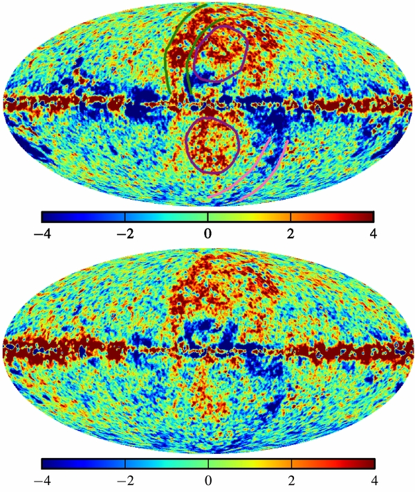
Figure 6. Residual maps in units of standard deviation in the energy range 200 MeV–100 GeV. Shown are residuals for model SSZ4R20T150C5 (top) and model SLZ6R20T∞C5 (bottom). The top map shows in addition a sketch of a few identified large-scale residuals, Loop I (green), Magellanic stream (pink), and features coincident with those identified by Su et al. (2010) and Dobler et al. (2010) (magenta). The maps have been smoothed with a 05 hard-edge kernel. The kernel is inclusive so that every pixel intersecting the kernel is taken into account.
Download figure:
Standard image High-resolution image
Figure 7. Fractional residual maps, (model-data)/data, in the energy range 200 MeV–100 GeV. Shown are residuals for model SSZ4R20T150C5 (top) and model SLZ6R20T∞C5 (bottom). The maps have been smoothed with a 05 hard-edge kernel; see Figure 6.
Download figure:
Standard image High-resolution imageAll of the models considered have large positive residuals at intermediate and high latitudes about the Galactic center, most notably features coincident with those described by Su et al. (2010) and Dobler et al. (2010), and a feature that is similar to the radio-detected Loop I (Casandjian et al. 2009). The negative residual of the Magellanic stream is also visible in the southern hemisphere. It was not subtracted from the H i annular column density maps because its contribution to the column density was incorrectly assumed to be negligible. However, this does not affect our model comparison because the models all include this same extra column density. Due to the limited freedom in our fits of the DGE to the γ-ray sky, no attempt will be made here to characterize these residual structures but we do note that their shapes depend on the assumed DGE model.
Point sources are also evident in the large-scale residuals, indicating that the point-source fluxes determined by the fit are biased in these areas. However, their PSF-like spatial extent prevents them from affecting the DGE modeling significantly. Only in areas with many overlapping point sources, such as in the Galactic ridge, can they mimic the structure of the DGE. Our tests have shown that inaccurate source modeling causes less than 20% variations in the derived XCO factors, less than the variation caused by the CR source distribution and gas properties (see Section 4.3).
The track of the Sun along the ecliptic can also be seen (particularly in the north), although it is not very prominent. The quiet Sun is a source of high-energy γ-rays from CR nuclei interacting in its atmosphere (Seckel et al. 1991) and CR electrons and positrons IC scattering of the heliospheric photon field (Moskalenko et al. 2006a; Orlando & Strong 2007, 2008; Abdo et al. 2011). However, when averaged over a year the overall intensity of this component is very small, being less than 5% of the isotropic background over most of the sky (Abdo et al. 2010g), and does not affect the large-scale DGE modeling significantly. The Moon also contributes to the emission from the ecliptic, being nearly as bright as the Sun around 100 MeV. But, the equivalent diffuse intensity from the moving Moon is less due to the inclination of its orbit relative to the ecliptic. The γ-ray spectrum from the Moon is also steeper than that of the Sun (Moskalenko & Porter 2007) and does not contribute at a detectable level above 10 GeV.
For comparisons between models, we calculate the differences between the absolute values of the fractional residual maps for the models. These maps show directly which model better fits the data while the difference between the models might be larger than shown in these plots. To study the effects of individual parameters, we compare models where only a single model grid parameter is varied. In Figure 8 we show the difference residual maps for variation of only the CR source distribution, changes in the size of the CR confinement volume in Figure 9, and variations of the gas properties in Figure 10. While only a single model grid parameter is changed between the models, there are related changes in the propagation parameters, CR source injection spectrum, ISRF scale factor, XCO factors, isotropic spectrum, and point-source spectra resulting from the CR and γ-ray fits that also affect the results. The variation of the gas-related parameters has the largest and most distributed effect across the sky. Varying the E(B − V) magnitude cut produces differences that are mostly confined to the Galactic plane, but the small change in the gas-to-dust ratio (see Table 2) has an effect at higher latitudes. Changing TS gives large positive and negative differences over the sky. The most striking feature is toward the outer Galaxy, where changing from TS = 150 K to the optically thin approximation mostly improves the agreement at intermediate latitudes, but generally worsens it in the outer Galaxy plane. The improvement at intermediate latitudes seems to correlate at least somewhat with the distribution of CO at intermediate latitudes seen in Figure 3, indicating that the gamma-ray signal is sensitive to the ratio of the gas-to-dust ratios for H i and CO. Another explanation might be a Galactocentric gradient of the gas-to-dust ratios, it being higher in the outer Galaxy in agreement with the increased metallicity in the outer Galaxy. Other variations at high latitude are not as strong but still significant. Due to the diffusive propagation of CRs throughout the Galaxy, the steady state CR distribution should not show strong variations on the scales that are needed to account for the differences shown in the figure. This indicates rather that the assumption of a single TS value, and hence gas-to-dust ratio, should be reconsidered in subsequent work.

Figure 8. Difference between the absolute values of the fractional residuals of models where only the CR source distribution is changed. Top: model SLZ10R30T150C5 minus model SOZ10R30T150C5; middle: model SLZ10R30T150C5 minus model SSZ10R30T150C5; bottom: model SLZ10R30T150C5 minus model SYZ10R30T150C5. Negative pixels represent a better fit with the first mentioned model. The maps have been smoothed with a 05 hard-edge kernel; see Figure 6.
Download figure:
Standard image High-resolution image
Figure 9. Difference between the absolute values of the fractional residuals of models where only the halo size is changed. Top: model SSZ4R20T150C5 minus model SSZ10R20T150C5; bottom: model SYZ10R20T150C2 minus model SYZ10R30T150C2. Negative pixels represent a better fit with the first mentioned model. The maps have been smoothed with a 05 hard-edge kernel; see Figure 6.
Download figure:
Standard image High-resolution image
Figure 10. Difference between the absolute values of the fractional residuals of models where only the properties of the gas distribution is changed. Top: model SSZ4R20T150C5 minus model SSZ4R20T∞C5; middle: model SYZ10R30T150C2 minus model SYZ10R30T∞C2; and bottom: model SSZ4R20T150C2 minus model SSZ4R20T150C5. Negative pixels represent a better fit with the first mentioned model. The maps have been smoothed with a 05 hard-edge kernel; see Figure 6.
Download figure:
Standard image High-resolution imageWhile variation of the assumed CR source distribution does not show as strong of an effect as for the gas properties, significant differences are still seen over the sky. No single CR source distribution is best for all regions of the sky. A strong asymmetric feature in the direction of the inner Galaxy can be seen in the top panel of Figure 8, having opposite signs above and below the plane, indicating a missing asymmetry in the model, either in terms of gas properties or CR flux. The outer Galaxy shows similar features, where the intermediate latitudes and the plane have opposite signs. This is most easily seen in the middle panel of Figure 8 where we have an improvement in the fit in the plane but worsening at intermediate latitudes. Because the SNR distribution provides more CR flux in the outer Galaxy, this indicates that the gas distribution could be more closely confined to the plane in the outer Galaxy than estimated in our modeling. This possibility has been studied by Kalberla et al. (2007) who found a reduced extension in z of the gas distribution in the outer Galaxy when assuming the gas in the halo rotated more slowly than gas in the plane.
Variation of the halo size parameters produces low-level residuals, both positive and negative, in different regions of the sky. The halo size, zh, has the strongest influence in the outer Galaxy and in the region above and below the Galactic plane in the direction of the Galactic center. The former can be explained by increased CR flux in the outer Galaxy when zh is increased, while the latter is due to increased IC emission in the direction of the Galactic center caused by a longer integration path length along the LOS. The increase in IC emission is suppressed somewhat because the normalization of the ISRF is anti-correlated with zh (see Section 4.4). Increasing Rh affects only the outer Galaxy significantly, where the models with larger Rh better agree with the data.
The effect of varying a single parameter on the derived residuals can be strongly interdependent on the other adopted input parameters. This is illustrated in Figure 10 where the difference in residuals when varying TS for two different sets of the other input parameters is shown. The changes are clearly different depending on the input parameters and the resulting parameters found from the CR and γ-ray fits.
Finally, to illustrate the differences between models where more than one parameter is changed, we compare in Figure 11 models SLZ6R20T∞C5, SYZ10R30T150C2, and SOZ8R30T∞C2 to the reference model SSZ4R20T150C5. The models were chosen to illustrate the range of our parameter scan. While some models fare better than others in the likelihood ratio tests (see Figure 4), there is no model that is uniformly better than the other models. There are large-scale positive and negative differences between the models that are distributed over the entire sky, although the greatest differences are at low latitudes. We emphasize that differences between models can be nonlinear, and caution should therefore be exercised when interpreting low-level residual structures because of subtle interplay between the different model parameters.

Figure 11. Difference between the absolute values of the fractional residuals of model SSZ4R20T150C5 and model SLZ6R20T∞C5 (top); model SSZ4R20T150C5 and model SYZ10R30T150C2 (middle); and model SSZ4R20T150C5 and model SOZ8R30T∞C2 (bottom). Negative pixels represent a better fit with model SSZ4R20T150C5, while positive pixels are better fit with the other models. The maps have been smoothed with a 05 hard-edge kernel; see Figure 6.
Download figure:
Standard image High-resolution image4.2.2. Plots of Spectra
We plot the spectra of models and data for several selected regions. It is evident from Figure 12 that the models give on average a good description of the Fermi-LAT data at high and intermediate latitudes. Even though the likelihoods of the models differ significantly, the model predictions for the total intensity fall within the systematic error of the Fermi-LAT effective area, deviating less than 10% from the data over the entire energy range. This is partly due to the freedom we have when fitting for the isotropic background (see Section 4.5). Figure 13 shows that we overpredict the data in the south polar cap, an indication that the isotropic component is too large and compensating for inaccuracies in the DGE models. But, even for the intermediate-latitude region shown in Figure 14, where the DGE dominates the isotropic component, the agreement is very good.

Figure 12. Spectra extracted from the local region for model SSZ4R20T150C5 (top) and model SOZ8R30T∞C2 (bottom) along with the isotropic background (brown, long-dash-dotted) and the detected sources (orange, dotted). The models are split into the three basic emission components: π0-decay (red, long-dashed), IC (green, dashed), and bremsstrahlung (cyan, dash-dotted). All components have been scaled with parameters found from the γ-ray fits. Also shown is the total DGE (blue, long-dash-dashed) and total emission including detected sources and isotropic background (magenta, solid). The Fermi-LAT data are shown as points and the error bars represent the statistical errors only that are in many cases smaller than the point size. The gray region represents the systematic error in the Fermi-LAT effective area. The inset sky map in the top right corner shows the Fermi-LAT counts in the region plotted. Bottom panel shows the fractional residual (data-model)/data.
Download figure:
Standard image High-resolution image
Figure 13. Spectra extracted from the polar cap regions, north (top) and south (bottom) for model SSZ4R20T150C5. See Figure 12 for legend. Note that the model shows a north–south asymmetry in the residuals that is most prominent at high energies but can be seen over the entire spectral range.
Download figure:
Standard image High-resolution image
Figure 14. Spectra of the low intermediate latitude region for model SSZ4R20T150C5 (top) and model SOZ8R30T∞C2 (bottom). This region was also used by Abdo et al. (2009a). See Figure 12 for legend.
Download figure:
Standard image High-resolution imageThe models in the current paper agree better with the intermediate-latitude data (Figure 14) than the model presented in Abdo et al. (2009a) for two main reasons. First, we use dust as an additional tracer for gas densities that has been shown to give better results than using only H i and CO tracers (Grenier et al. 2005). This is especially true for intermediate latitudes in the direction toward the inner Galaxy, which is the brightest part of the low intermediate-latitude region. Second, we allow for freedom in both the ISRF scale factor and XCO to tune the model to the data, which is well motivated given the uncertainty in those input parameters.
The models in general do not fare as well in the Galactic plane where they systematically underpredict the data above a few GeV but overpredict it at energies below a GeV. This is most pronounced in the inner Galaxy (Figure 15), but can also be seen in the outer Galaxy (Figure 16), with even a small excess at intermediate latitudes (Figure 14). Possible explanations for this discrepancy are deferred to the discussion section. We note that the dip in the data visible between 10 and 20 GeV is due to the IRFs used in the present analysis. Figure 17 shows a comparison of model SSZ4R20T150C5 to the data in the outer Galaxy using the Pass 7 clean photons. The dip between 10 and 20 GeV is greatly reduced because of the improved effective area of the new photon class. Because our results do not depend strongly on the exact shapes of the spectra of the data, these improvements in the effective area do not affect our conclusions.

Figure 15. Spectra extracted from the inner Galaxy region for model SSZ4R20T150C5. See Figure 12 for legend.
Download figure:
Standard image High-resolution image
Figure 16. Spectra extracted from the outer Galaxy region for model SSZ4R20T150C5 (top left); SOZ10R20T150C5 (top right); SSZ4R20T∞C5 (bottom left); and SOZ4R20T150C5 (bottom right). See Figure 12 for legend.
Download figure:
Standard image High-resolution image
Figure 17. Spectra extracted from the inner Galaxy region for model SSZ4R20T150C5 using Pass 7 clean photons. The dip between 10 and 20 GeV is greatly reduced compared to Figure 15. See Figure 12 for legend.
Download figure:
Standard image High-resolution imageThe maximum-likelihood trend of preferring models with larger zh, lower TS, and flatter CR source distribution (see Figure 4) is illustrated in Figure 16. Going from the SNR distribution to the OB star distribution has very similar effects as changing from TS = 150 K to the optically thin approximation and also increasing zh from 4 kpc to 10 kpc. We note that changing zh with the SNR distribution has a much smaller effect. It is also evident that all of the models underpredict the data in this region above ∼800 MeV, and some even for the entire energy range.
4.2.3. Longitude and Latitude Profile Plots
We compare longitude and latitude profiles of representative models and data for selected regions. For the profile plots, we use three energy bands (200 MeV–1.6 GeV, 1.6–13 GeV, and 13–100 GeV) to increase the statistics in the profiles. Our discussion below is mainly focused on the lowest energy band, because this has the highest statistics and even though the PSF is broader than at higher energies the profiles are wide enough to be relatively unaffected. In general, the models agree well with the data, deviating less than ∼10% from the data over a large fraction of the sky while covering almost two decades of dynamic range in the latitude profiles. From the profile figures, the component associated with CRs interacting with the H i dominates the DGE in most sky regions and for most of the energy range of the Fermi-LAT. The IC component approaches a similar intensity to the H i for high latitudes, and dominates only in the 13–100 GeV energy band. The H2 component extends only a few degrees from the Galactic plane and is dominant only in the inner Galaxy.
Despite the overall good agreement, the profile residuals do show structure on scales from few degrees to tens of degrees. For the latitude profile in the outer Galaxy shown in Figure 18, it is evident that the models underpredict the data in the Galactic plane, but overpredict it at intermediate latitudes. The exact shape and magnitude of this residual depend on the model. The underprediction in the plane is mostly dependent on the CR flux in the outer Galaxy (CR source distribution and halo height), while the overprediction at intermediate latitudes depends mostly on the assumed TS value and therefore gas-to-dust ratio (see Section 3.3.4). These effects can be seen also toward the inner Galaxy (Figure 19), but the effect is mostly absent toward the Galactic center (Figure 20). The residual map differences in Figures 8 and 10 also illustrate this.

Figure 18. Latitude profile showing the outer Galaxy in the energy range 200 MeV–1.6 GeV. Shown are profiles for models SSZ4R20T150C5 (top left), SLZ6R20T∞C5 (top right), SYZ10R30T150C2 (bottom left), and SOZ8R30T∞C2 (bottom right). The DGE model is split into the three different gas components: H i (red, long-dashed), H2 (cyan, dash-dotted), and H ii (pink, long-dash-dash-dotted), and also IC (green, dashed). Also shown are the isotropic component (brown, long-dash-dotted), the detected sources (orange, dotted), total DGE (blue, long-dash-dashed), and total model (magenta, solid). Fermi-LAT data are shown as points with statistical error bars and the systematic uncertainty in the effective area is shown as a gray band. Due to the evenness of the sky exposure of the Fermi-LAT, the systematic error is not expected to be position dependent, only global normalization for the profile. The inset sky map in the top right corner shows the Fermi-LAT counts in the region plotted. The bottom panel shows fractional residuals (data-model)/data.
Download figure:
Standard image High-resolution image
Figure 19. Latitude profile for model SSZ4R20T150C5 showing the inner Galaxy without the inner ±30° about the Galactic center for 200 MeV–1.6 GeV. See Figure 18 for legend.
Download figure:
Standard image High-resolution image
Figure 20. Latitude profile for model SSZ4R20T150C5 showing the innermost l ± 30° about Galactic center for 200 MeV–1.6 GeV (top), 1.6 GeV–13 GeV (middle), and 13 GeV–1000 GeV (bottom). See Figure 18 for legend.
Download figure:
Standard image High-resolution imageThe dip around the Galactic plane in the residual in Figure 18 is caused by unreasonably large XCO factors found from the fits (see Section 4.3), artificially increasing the H2 component. A residual structure coincident with the H2 component is not seen in any of the other latitude profiles. The underprediction in the outer Galaxy can also be seen in the longitude profiles in the Galactic plane (Figure 21) where peaks in the H2 component corresponds with dips in the residual. The contribution from detected point sources is also strongest in the plane with a similar profile as the H2 component, which can also compensate for a lack of freedom in the DGE model during the fitting procedure. The longitude profile in the Galactic plane does not show a correlation of peaks in the source intensity and dips in the residual indicating that sources from the 1FGL catalog are not able to compensate for large-scale inaccuracies in the diffuse emission.

Figure 21. Longitude profile showing the Galactic plane in the energy range 200 MeV–1.6 GeV. Shown are profiles for model SSZ4R20T150C5 (top left), SSZ4R20T150C2 (top right), SSZ4R20T∞C5 (bottom left), and SLZ4R20T150C5 (bottom right). See Figure 18 for legend.
Download figure:
Standard image High-resolution imageAll of the latitude profiles display a north–south asymmetry in the residuals, as was shown in the spectra of the polar cap regions in Figure 13. The effect is most noticeable in Figure 19, which is caused mostly by the gas from the Magellanic stream (Mathewson et al. 1974) that was not removed from the H i annular column density maps as mentioned earlier. As the north–south asymmetry is also visible in the outer Galaxy profile where the Magellanic stream has very little effect, there must be some underlying asymmetry. The origin of this asymmetry is not currently known. It is more likely associated with an asymmetry in the CR flux rather than the ISM because the ISM is more observationally constrained.
The model underprediction above a few GeV seen in Figures 15 and 16 is confined to the Galactic plane, as can be seen in Figure 22. The model systematically underpredicts the data in the plane in the 1.6–13 GeV and 13–100 GeV energy bands, but very little excess emission is seen at higher latitudes. This is not seen as clearly in the Galactic center profile (Figure 20) because that region also includes other large-scale residuals, most notably due to features coincident with those described by Su et al. (2010) and Dobler et al. (2010). Note that while these are prominent above 1.6 GeV, they can also be seen at lower energies, but the details of the residual features depend on the DGE model.

Figure 22. Latitude profile showing the outer Galaxy in the 1.6–13 GeV (top) and 13–100 GeV (bottom) energy range for model SSZ4R20T150C5. See Figure 18 for legend.
Download figure:
Standard image High-resolution imageFigure 21 shows the longitude profile about the Galactic plane for a few different models. It shows how the H i component is affected by different assumptions for TS, the magnitude cut in the dust map, and the different CR source distributions. The difference in the CR source distribution is also seen in the IC component that is more peaked for the Lorimer source distribution than the SNR distribution. This can be better seen at intermediate latitudes in Figure 23. The effect is noticeable both at intermediate latitudes as well as in the outer Galaxy where CO from the local annulus dominates.

Figure 23. Longitude profile for models SSZ4R20T150C5 (top) and SLZ4R20T150C5 (bottom) showing south intermediate latitudes in the energy range 200 MeV–1.6 GeV. See Figure 18 for legend.
Download figure:
Standard image High-resolution imageThe residuals in the plane show signs of small-scale features that are not compatible with statistical fluctuations. Similar residual structure is also seen at intermediate latitudes in Figures 23 and 24, where the most significant structures in the residuals are correlated with peaks in the H i distribution. Note that some peaks in the H i distribution are not associated with residual structure. It is unlikely that the small angular scale fluctuations are due to small-scale CR intensity variations because the bulk of the CR nuclei producing the DGE for the energy range shown are smoothly distributed. The variations are then mostly caused by features in the annular gas maps that introduce artifacts on small angular scales. This suggests that the gas-to-dust ratio is not constant over the sky and can fluctuate by at least 10%. However, comparing the panels in Figure 24, the residual structure can be seen to be energy dependent. The largest variation is toward the inner Galaxy that can be associated with structure coincident with those identified by Su et al. (2010) and Dobler et al. (2010) but smaller variations around l = 100° indicate spectral variations in the CR flux. See, e.g., Bykov & Fleishman (1992) for how OB associations and super-bubbles might have an effect on the CR flux on smaller spatial scales.

Figure 24. Longitude profile for model SSZ4R20T150C5 showing north intermediate latitudes in the energy range 200 MeV–1.6 GeV (top) and 1.6 GeV–13 GeV (bottom). See Figure 18 for legend.
Download figure:
Standard image High-resolution image4.3. Radial Dependence of XCO
Figure 25 shows the radial dependence of XCO for a few selected models. XCO for all models can be found in the online supplementary material. Our analysis finds that XCO(R) depends both on the assumed CR source distribution and the gas properties. This is illustrated in Figure 26, which shows XCO derived for the local annulus for all models. The local XCO varies by up to a factor of two depending on the value of TS and the E(B − V) magnitude cut but is nearly independent of the other input parameters. Because the emissivity of the local gas is well determined by observations of CRs, this shows that an accurate determination of the H i column density is important for determining XCO values from γ-ray data.

Figure 25. Radial distribution of XCO for model SSZ4R20T150C5 (black X), SLZ6R20T∞C5 (blue squares), SYZ10R30T150C2 (red circles), and SOZ8R30T∞C2 (green triangles). We do not show the XCO values in the outer Galaxy because they are strongly biased by the lack of γ-ray intensity in the outer Galaxy in our models. For comparison, we also show data from Abdo et al. (2010d; purple diamonds), Ackermann et al. (2011b; cyan stars), and Strong et al. (2004c; solid curve). The blue dashed curve shows the initial value we used in our iterative procedure.
Download figure:
Standard image High-resolution image
Figure 26. Determined values of XCO associated with the local annulus for all models. See Figure 4 for legend.
Download figure:
Standard image High-resolution imageThe scatter in the XCO is not surprising. The limited freedom in the γ-ray fit can bias the derived values as has already been mentioned. For XCO the bias can be twofold. For an accurate determination of XCO we need to know the γ-ray intensity associated with CO as well as the emissivity per H2 atom. For our case, we calculate the emissivity assuming a CR distribution and estimate the intensity from a fit to the γ-ray data. If the emissivity is incorrectly estimated, the intensity associated with CO will be biased in the opposite direction, resulting in the twofold bias. Methods that determine the emissivity of the gas simultaneously with the intensity associated with CO are independent of this bias, as long as the emissivity is accurately determined from the data (e.g., Abdo et al. 2010d; Ackermann et al. 2011b). Note that the effect of variations in N(H i) applies in all cases. However, the scatter in the XCO we determine does not significantly affect our comparison between the models except possibly in the inner Galaxy where the molecular gas content is greatest.
Despite the large variations of the XCO factors between the models there are several features that are consistent. The XCO factors in the inner Galaxy are systematically higher than the estimate from Strong et al. (2004c), even when using the same CR source distribution. Only in the innermost annulus is there agreement between our XCO values and those of Strong et al. (2004c). The strong decrease of XCO in the innermost annulus is consistent for all our models as has also been seen in other analyses (see, e.g., Ferrière et al. 2007). This has been attributed to the breakdown of XCO as a tracer of H2 because the 12CO line becomes less optically thick in the Galactic center region (Dahmen et al. 1998). There also seems to be a dip in XCO for the local annulus that was not in Strong et al. (2004c). Our values for the local region XCO agree very well with the value found for the nearby Gould Belt by Abdo et al. (2010d). Because the XCO values for this annulus are determined from fits to the local region, the value is associated with high-latitude clouds. This indicates that molecular clouds in the vicinity of the solar system may have different properties than clouds at a similar Galactocentric distance. High-latitude translucent clouds have also been shown before to have lower XCO values (de Vries et al. 1987; Heithausen & Thaddeus 1990), but more recent work based on other tracers of molecular hydrogen shows that CO intensities might not be linearly related to H2 column densities in those clouds (Magnani et al. 2003).
There is an exponential increase in the outer Galaxy that is strongly dependent on the assumed CR source distribution, halo size, and TS. Figure 27 shows the fractional residual (see Section 4.2) for model SSZ4R20T150C5 with the integrated CO emission in the outer Galaxy overlaid. A correlation between the CO emission and negative residuals is evident. On this basis, we conclude that the XCO values in the outer Galaxy derived in our analysis are strongly biased and we do not show them in Figure 25. This bias is caused by the underprediction of γ-ray intensity in the outer Galaxy by all of the models considered here. Because there is very little CO in the outer Galaxy (see Figure 3) this bias will not strongly affect our results, but only slightly reduce the scatter when comparing the models in the outer Galaxy.

Figure 27. Relative residual (data-model)/data for model SSZ4R20T150C5. Overlaid are contours for the integrated CO emission in the outer Galaxy (R > 10 kpc) at 2 K km s−1 (magenta) and 5 K km s−1 (white). The CO is clearly correlated with negative residuals in the map, indicating that our XCO factors in the outer Galaxy are overestimated. Note that the latitude scale is stretched two times compared to the longitude scale for clarity.
Download figure:
Standard image High-resolution image4.4. ISRF Scaling Factors
The scaling factor of the ISRF is shown in Figure 28 for each model in both the local and inner region. The derived ISRF scaling factor is model dependent and varies with CR source distribution, gas densities, and halo size. In general, the scaling factor is smaller for the pulsar CR source distributions that are more peaked toward the inner Galaxy than both the OB stars and SNR distributions. More CRs will be injected in the inner Galaxy from the pulsar-like source distributions. This produces a corresponding increase in the IC emission in this region because of the larger number of CR electrons and positrons for these source distributions.

Figure 28. Scaling factor of the ISRF resulting from the fits in the local region (upper panel) and inner region (lower panel). See Figure 4 for legend.
Download figure:
Standard image High-resolution imageThe ISRF scaling factor is also dependent on TS and the E(B − V) magnitude cut, indicating that the normalization of the ISRF (and of the IC intensities) serves to compensate for different gas densities in the fits. This is despite the IC component being both spectrally and also spatially different from the H i component. The latitude dependence of the IC component is similar enough to the H i component (see Figure 20) to allow for the correlation between the H i and IC components in the fit. Coupling that with the trend between increased likelihood in the inner region for the optically thin case seems to indicate that a greater intensity of IC is needed for all models, either from an increased ISRF, more CR electron sources, or a larger zh. The longer confinement time for the CR electrons/positrons for the larger halo sizes, together with the approximately 1/z decrease of the ISRF perpendicular to the Galactic plane (Porter et al. 2008), produces more IC emission for cases with larger zh (see also Strong et al. 2010). This effect can be seen as a decrease in the scaling factor in the local region with increasing zh, although the magnitude of the decrease depends on the assumed CR source distribution and gas densities. The ISRF scaling factors follow a trend in that they are larger for the inner Galaxy region for larger zh. This indicates that further enhancement is required in addition to that provided by the large zh, which could be due to additional CR electrons/positrons, or an increase in the ISRF in the inner Galaxy region. Disentangling these effects is difficult. One way could be to consider the IC from CMB photons along with the bremsstrahlung emission. Unfortunately, their overall intensity is not high enough to allow them to be used to constrain the CR electron component. The ISRF scaling factors therefore only allow us to infer that the IC modeling requires modifications but a detailed investigation is needed to unravel their origin.
4.5. Isotropic Background
The spectrum of the derived isotropic background is shown in Figure 29 for selected models. Isotropic spectra for all models can be found in the online supplementary material. As for the ISRF normalization and XCO values, the isotropic background is model dependent. However, the variation in the overall normalization is not very large because it is spatially very different from the other fitted components. The derived spectral shape is also very similar amongst the various models. Both of these indicate that the isotropic background is not strongly biased by variations between the different models.

Figure 29. Spectra of the isotropic component determined from the local region fit for model SSZ4R20T150C5 (black X), SLZ6R20T∞C5 (blue squares), SYZ10R30T150C2 (red circles), and SOZ8R30T∞C2 (green triangles). The gray shaded area is the isotropic component from Abdo et al. (2010g) combining their EGB and residual component, including the effective area systematic uncertainty. Other systematic uncertainties estimated by Abdo et al. (2010g) are not included in the figure. Their magnitude could be comparable to the effective area systematic uncertainty.
Download figure:
Standard image High-resolution imageFigure 29 also shows a comparison with the isotropic spectrum from Abdo et al. (2010g) after combining the derived EGB and RIB components from that work. Our estimates of the isotropic background are consistent with Abdo et al. (2010g) below 1 GeV, and systematically higher above this energy. Despite our efforts to minimize the contribution of the Galactic ridge to the determination of the isotropic background by fitting for the local region, Figure 14 shows that the model slightly underestimates the data at low intermediate latitudes above 1 GeV while still being within the systematic uncertainty of the Fermi-LAT data. The fit will compensate for this with the isotropic component as can be seen in Figure 13 where the model overestimates the data in the polar cap regions above 1 GeV. This is especially true in the south polar cap. The difference in the two estimates of the isotropic background can therefore be attributed to the additional freedom allowed in the diffuse Galactic emission model in the analysis of Abdo et al. (2010g) where the intensity spectrum of the local H i annulus and the IC component was allowed to vary freely. The motivations for this additional freedom were the uncertainties associated with the observed CR intensities that are around few percent at energies above 100 GeV reaching more than 10% below 10 GeV caused by the uncertainty in solar modulation, and the size of the CR halo. The combination of these can produce variations both in the H i-related and IC emission. Because our models predict the Fermi-LAT data within the systematic error we do not try to account for this uncertainty in this analysis. The isotropic spectrum from Abdo et al. (2010g) is therefore a better measurement. This does not affect the comparison between the models considered in this paper because they are all treated identically.
4.6. CR Propagation Parameters
Because the main purpose of the fit to CR data is to obtain a propagation model consistent with CR observations, we defer most of the discussion of the results to Appendix D and only summarize the few key points here. We emphasize that all the models give a good representation of the CR data as can be seen in Figures 30 and 31. This has been shown earlier for similar diffusive-reacceleration models (Strong & Moskalenko 1998). But models with zh = 10 kpc are at the limit of consistency with the observed 10Be/9Be ratio and therefore considering larger values for zh is not warranted.

Figure 30. Comparison of model SSZ4R20T150C5 (black solid curve), SLZ6R20T∞C5 (blue dashed curve), SYZ10R30T150C2 (red dotted curve), and SOZ8R30T∞C2 (green dash-dotted curve) to CR observations. Shown are protons (top left), helium (top right), electrons (bottom left), and electrons and positrons (bottom right). In addition to the data we used for the CR fit (see Section 3.2) we also show data from PAMELA (Adriani et al. 2011a, 2011b), ATIC-2 (Wefel et al. 2008), and CREAM (Yoon et al. 2011). Error bars for the x-axis indicate bin width and error bars for the y-axis include systematic error. Models are corrected for solar modulation with the appropriate modulation potential found either from the CR fits and shown in Figure 36 or with the fixed values given in Section 3.2. Because Fermi-LAT and H.E.S.S. cannot discriminate between positrons and electrons the model total electron + positron spectrum is compared to the data. The positron component of the model is shown as the thick line, which is corrected with a modulation potential of 300 MV. The interstellar spectra are shown as the thin curves.
Download figure:
Standard image High-resolution image
Figure 31. Comparison of model SSZ4R20T150C5 (black solid curve), SLZ6R20T∞C5 (blue dashed curve), SYZ10R30T150C2 (red dotted curve), and SOZ8R30T∞C2 (green dash-dotted curve) to CR observations of B/C ratio (top), and 10Be/9Be ratio (bottom). In addition to the data we used for the CR fit (see Section 3.2) we also show data from CREAM (Ahn et al. 2010), ACE (Yanasak et al. 2001), and ISOMAX (Hams et al. 2004). Error bars for the x-axis indicate bin width and error bars for the y-axis include systematic error. Models are corrected for solar modulation with the modulation potential shown in Figure 36. 10Be/9Be ratio uses modulation for ACE. For a direct comparison, we also show the interstellar spectrum of the components as thin curves.
Download figure:
Standard image High-resolution imageThe propagation parameters from the fits shown in Figures 32 and 33 are generally in agreement with values found from similar analyses (Strong et al. 2004a; Trotta et al. 2011). The values are also stable between the different models, with notable exceptions for D0 and vA. These parameters are strongly correlated with zh and the properties of the gas distribution, that is, the XCO profile.70 The values of D0 and vA are also slightly affected by the assumed CR source distribution. Therefore, the values for these parameters should be interpreted in the context of the entire model that they were determined from because they depend not only on the propagation set up, but also on the distributions of gas and assumed CR sources.

Figure 32. Resulting propagation parameters from the fit to CR nuclei data. Top shows D0 and bottom shows vA.
Download figure:
Standard image High-resolution image
Figure 33. Resulting propagation parameters from the nuclei fit. Shown are low-energy nuclei index (top left), high-energy nuclei index (top right), nuclei break rigidity (bottom left), and proton normalization (bottom right). See Figure 4 for legend.
Download figure:
Standard image High-resolution image5. DISCUSSION
The agreement between all of our models and the Fermi-LAT data is, on average, good despite minimal fitting. The models generally agree within ≈15% of the data over most of the sky except for regions discussed below. In Figure 34 we show the predicted emissivities of the local annulus for a few example models and compare them with emissivities derived from the Fermi-LAT data using different methods (Abdo et al. 2009b, 2010d; Ackermann et al. 2011b). The agreement is in line with our results from the local region; the models predict the local emissivities within the scatter of the observations. The scatter between different Fermi-LAT results is most likely caused by uncertainties in the column densities of gas used in the template fitting.

Figure 34. Average emissivity of the local annulus for model SSZ4R20T150C5 (solid black), SLZ6R20T∞C5 (blue dashed), SYZ10R30T150C2 (red dotted), and SOZ8R30T∞C2 (green dash-dotted). Shown for comparison are emissivities derived from Fermi-LAT data using a template fitting approach. Cyan stars are from Ackermann et al. (2011b), magenta diamonds are from Abdo et al. (2010d), and black squares are from Abdo et al. (2009b).
Download figure:
Standard image High-resolution imageThe parameter scan was deliberately limited due to computational constraints. However, it does provide insight into the effects associated with the variations of different parameters. For a given assumption on the CR propagation model, variations of the gas-related parameters give the largest variations in log-likelihoods for the γ-ray fit over the entire sky. The CR source distribution and halo size, however, show such large effects on the likelihood ratio in the outer Galaxy only. Similarly, the gas-related parameters have a large effect on the residual sky maps at all angular scales, which contrasts with the much smoother structures caused by changes in the assumed CR source distribution and size of the confinement volume. Understanding the Galactic gas distribution and its different phases is essential for accurate modeling of the DGE.
The most important parameter in our scan is the H i spin temperature used for the optical depth correction for deriving N(H i). For our analysis, we considered two values, TS = 150 K and TS very large (i.e., the optically thin approximation). This is a highly simplified approach because observations show that TS varies from 10s to 1000s of K (e.g., Dickey et al. 2009). A preliminary study showed that alternative approximations for the value of TS can significantly improve the agreement between DGE models and Fermi-LAT data (Johannesson et al. 2010). Further improvements include taking into account H i self-absorption (Gibson 2002, 2010) and uncertainties in the rotation curve for the H i distribution, which will be explored in future work.
We confirm the need for augmenting the use of CO and H i line observations as tracers of the interstellar gas with infrared observations of interstellar dust (Grenier et al. 2005; Abdo et al. 2010d; Ackermann et al. 2011b; Planck Collaboration et al. 2011). Dust reveals some molecular hydrogen that is not traced by CO which can compensate to some extent for errors in or variations of the spin temperature of the interstellar hydrogen. The dust column density is represented in this work as the equivalent interstellar reddening E(B − V) and limitations of the color correction method used to derive the reddening maps make them less accurate near the Galactic plane. But our analysis shows that the γ-ray fit improves with the inclusion of dust near the Galactic plane, up to a reddening magnitude of 5. The disadvantage of E(B − V) as a tracer of interstellar gas is that it provides no distance information analogous to the Doppler shifts of the CO and H i lines due to differential rotation of the Milky Way, and for this work we distributed the "excess" E(B − V)-associated column densities like the inferred distribution of H i. This distribution of the "excess" is reasonable in regions with little or no CO emission but is suspect near large molecular clouds, where the "excess" should be mostly low-density H2 gas not traced by CO (e.g., Glover & Mac Low 2011).
The models all underpredict the data in the Galactic plane (Figure 16) above a few GeV and the difference is most pronounced in the inner Galaxy (Figure 15). The magnitude of the difference is much less than the so-called EGRET "GeV excess" and is also confined to the plane. A possible explanation for this is a contribution by point sources such as pulsars, SNRs, and pulsar wind nebulae (PWN). Only a fraction of these are actually detected individually by Fermi-LAT. The contribution by source populations below the detection threshold is currently undetermined and it may have a diffuse-like spatial distribution. A study of this topic based on EGRET data, with predictions for the Fermi-LAT, was made by Strong (2007), giving estimates of a ∼10% contribution by sources below the Fermi-LAT detection threshold. Pulsars are the largest contributor to detected Galactic sources in the 2FGL catalog (Nolan et al. 2011), being far more numerous than SNRs and PWN. This class might dominate the contribution by undetected sources, but due to their spectral cutoffs above ∼10 GeV they cannot completely explain the spectral difference that we find at higher energies. This will be addressed in a subsequent paper, employing a population-synthesis approach and comparison with the 2FGL catalog to constrain possible source contributions.
Another possibility is that the inner Milky Way contains fresh CR sources with a harder spectrum in addition to the presumed steady state CR population that has undergone propagation. Signs of freshly accelerated CRs have been recently observed in the Cygnus region (Ackermann et al. 2011a) and more regions are likely to be discovered in the future. Observations with H.E.S.S. of the Galactic plane at TeV energies may partly support this explanation. The H.E.S.S. observations showed γ-ray emission associated with molecular clouds that have harder spectra than expected from extrapolation of lower-energy spectra (Aharonian et al. 2006). However, freshly accelerated CRs are an unlikely explanation for the excess emission in the outer Galaxy. Another alternative is that local CR measurements do not sample the average CR spectra in the Galaxy (e.g., Porter & Protheroe 1997; Strong et al. 2004b). As discussed in Section 4.5, the uncertainties in the observed CR intensities have not been propagated to the DGE models. A 10% decrease in γ-ray intensity below 1 GeV and a few-percent increase above 1 GeV with additionally an overall increase in the total CR intensity would make the model agree with the data. The current analysis cannot distinguish between these alternatives, and most likely a combination will contribute to providing the required additional γ-ray emission.
Contrasting with the underprediction at ≳few GeV, the models overpredict the data at lower energies with the largest residual in the 200–400 MeV bin. While being most prominent in the inner Galaxy (Figure 15), this can also be seen to a lesser extent at low intermediate latitudes (Figure 14). The overprediction at low energies is fractionally smaller than the underprediction at higher energies and is partly contained within the systematical uncertainty of the effective area of the Fermi-LAT. We note, however, that the discrepancy is still visible using the updated instrument response in the Pass 7 event selection (Figure 17), suggesting that the effect is not entirely instrumental. The effect is strongest in the plane indicating that the π0-decay spectrum is primarily responsible for the mismatch. The γ-rays below ≲ 1 GeV are produced mainly by CR protons with energies ≲ 10 GeV. The locally measured CR proton spectrum (Figure 30) for these energies is affected by the solar modulation and is therefore subject to any errors we make in correcting for this effect. While the force-field approximation used in this paper is a useful parameterization, realistic models of the heliospheric CR transport (e.g., Florinski et al. 2010; Ngobeni & Potgieter 2010) could allow better determination of the low-energy interstellar CR nuclei spectra that are relevant for the calculation of the π0-decay γ-ray emission in our DGE models. The force-field approximation is, however, sufficient for the analysis done in this paper as we are mainly concerned with comparing the models with each other. Finally, we note that reducing the spectrum below 1 GeV and using a higher overall normalization for the CR nuclei results in an increase in the π0-decay DGE spectrum above ≳ 1 GeV. Therefore, the excess above a few GeV can also be partly due to uncertainties in how the solar modulation is handled when fitting to the observed CR spectra.
Despite the good agreement between model and data on average, there are structures seen on both small and large scales in the residual sky maps (Figure 7). Small-scale discrepancies are inevitable for any large-scale GALPROP-based model because simplifications have to be made to treat the CR transport together with the CR source, gas, and ISRF distributions. In particular, the assumption of axisymmetry for the CR source distribution and the ISRF is not a realistic model for the 3D distribution. Apart from Loop I, the Magellanic stream, and the structures coincident with the features found by Su et al. (2010) and Dobler et al. (2010), the most prominent of the large-scale residuals is the excess in the outer Galaxy. Our analysis shows that the observed intensities in the outer Galaxy are greater than predicted using conventional choices for the values of the parameters that we studied. Despite differing by more than a factor of three in CR density outside of 10 kpc, all of the CR source distributions considered in this paper give a model that underpredicts the observed γ-ray emissivity in the outer Galaxy. The models all show an increased likelihood for larger zh (Figure 4), which has been shown to increase the CR flux in the outer Galaxy (Abdo et al. 2010d; Ackermann et al. 2011b), but the large values of zh are approaching the bounds for consistency with the observed 10Be/9Be ratio (Figure 31). Another possibility is to increase the density of CR sources in the outer Galaxy. This would mean that SNRs, or CR source classes having a similar spatial distribution as the proxies considered in this paper, are not the only source of CRs (Butt 2009). Modifications of the CR propagation mechanism have also been proposed in the literature as an explanation for increased CR flux in the outer Galaxy (Breitschwerdt et al. 2002; Shibata et al. 2007). Alternatively, large amounts of gas not traced by 21 cm emitting H i and CO (as the tracer of H2) surveys may be present in the outer Galaxy (Papadopoulos et al. 2002), which would also increase the γ-ray emission. Breaking this degeneracy and deriving the correct CR source distribution and propagation model requires using all available data for CRs and their interactions in the ISM. Such a determination would inevitably have to take into account uncertainties involved in the astrophysical input to the models discussed in this paper.
The increase in log-likelihood for larger values of zh is also seen in the local region (Figure 4). An increase in zh is accompanied by a decrease in the ISRF scaling factor (Figure 28), indicating that additional IC emission at high latitudes is needed compared to the previously assumed zh = 4 kpc propagation models (e.g., Strong et al. 2004a). The longer confinement time for the CR electrons/positrons in the larger-halo-sized models results in more IC emission for these cases. From our analysis, the derived normalization of the IC component and its intensity varies considerably between CR source distributions. Because the spectral shape of the normalized IC emission is similar in all cases, the spatial distribution of this component determines the inferred IC contribution to the DGE for each model. This emphasizes that accurate modeling of the spatial distribution of the IC emission is essential to properly assess its intensity and spectrum from γ-ray data.
We have also explored how the uncertainties affect the CR propagation (Figure 32), aiming for a self-consistent model by incorporating the XCO values found from the γ-ray fit into the propagation parameter determination and transport calculations. Self-consistency, as used in this paper, is intended to ensure that the CR secondary-to-primary ratios and other direct measurements are consistent with the assumed TS and fitted XCO, which affect the gas density and hence CR secondary production. For an assumed set of input parameters, this is obtained by adjusting the spatial and momentum-space diffusion coefficients via D0 and the Alfvén speed vA, respectively. For the CR protons and He the propagated CR intensities and spectra are determined mostly by the assumed CR source distribution and boundary conditions because their energy loss timescales for the energies of interest in this paper are long compared to the propagation timescale. The CR electrons and positrons are more strongly affected by changes in the diffusion coefficient and halo size because their energy losses are much faster. The modeled CR intensities and spectra are also constrained by their normalization to the locally measured data, so the self-consistency requirement does not significantly change the γ-ray models and results for these models in this paper. Nevertheless, it is an important criterion to ensure that the origin of systematic effects from the assumed input parameters can be properly attributed. It is important to also emphasize that uncertainties in the input parameters can also affect the determination of the propagation parameters. Simply assuming that one set of propagation parameters applies equally to all variations of, e.g., assumed CR source distributions, is incorrect. Note that even though we have assumed a diffusive-reacceleration model for the CR propagation, this applies to the other variants such as pure diffusion models, models with convection, and so forth.
6. SUMMARY
This paper presents a systematic study of several basic parameters for global models of the DGE using Fermi-LAT data. The parameters, all inputs to the GALPROP CR propagation code, are related to the distributions of interstellar gas and of CRs, and for each combination of parameters considered the models were calculated self-consistently and were constrained to be consistent with local measurements of CRs. The evaluation of the models with respect to the data, taking into account the point sources in the 1FGL catalog, was made with the GaRDiAn software package, which was developed for studying diffuse emission in the Fermi-LAT data.
We find that augmenting the CO and H i column density estimate with column density estimates from dust improves agreement between model and γ-ray data. Our analysis finds this to be true even near the Galactic plane, where the dust column density estimated from the equivalent interstellar reddening E(B − V) is less accurate due to the limitations of the color correction method used to derive the reddening maps.
The DGE in the outer Galaxy is better fit by models with larger-than-expected CR halo sizes. There are other possibilities for the models to predict large enough intensities in the outer Galaxy. These include modifications of the assumed distributions of CR sources or of propagation of CRs in the outer Galaxy, or even the presence of much greater amounts of interstellar gas than currently assumed.
From our γ-ray fits in the region with |b| > 8° we show that larger IC intensities provide a better fit to the data for most models. In our approach, the single normalization factor for the optical and IR components of the ISRF that is shown to decrease with larger halo size provides this information. In addition to accounting for uncertainties in the ISRF, this normalization factor also encapsulates uncertainties in the distribution of CR electrons in the Galaxy.
All of the models considered in the paper underpredict the data above a few GeV in the Galactic plane. The magnitude of the difference is much less than the "GeV excess" observed by EGRET and mostly confined to the Galactic plane. Two possible explanations were discussed, contribution from undetected sources and variations in the CR spectra. Further analysis is needed to estimate the contribution from each.
We derived the radial distribution of XCO for all models and confirmed the systematically lower values of XCO for the innermost annulus (0–1.5 kpc). The XCO determined for the local annulus (8–10 kpc) above 8° latitude was also systematically lower than for the rest of the Galaxy, implying that the local high-latitude clouds have different properties than the Galactic average. Our XCO values for other radial ranges show that accurate determination of the CR gradient and the column density of the H i gas distribution are essential in determining the XCO gradient from γ-ray observations.
Our fits to the γ-ray data reveal the difficulties in accurately determining the properties of the ISM or CR propagation with DGE modeling. The derived XCO values and ISRF scaling parameters depend strongly on the assumed input parameters, both on the propagation setup and also on the properties of the H i gas distribution. Past studies using γ-ray data to determine these properties were thus susceptible to unexplored systematic uncertainties. The measured properties of Galactic plane sources even well above the detection limit can be affected by the assumed DGE model, especially for energy ranges where the scale of the PSF is comparable to the scale of the structure in the DGE. Accounting for systematic uncertainties of the astrophysical input needed for a DGE model is a necessary step in accurate analysis of γ-ray data when the observed signal is comparable or less than the DGE.
The Fermi-LAT Collaboration acknowledges generous ongoing support from a number of agencies and institutes that have supported both the development and the operation of the Fermi-LAT as well as scientific data analysis. These include the National Aeronautics and Space Administration and the Department of Energy in the United States, the Commissariat à l'Energie Atomique and the Centre National de la Recherche Scientifique/Institut National de Physique Nucléaire et de Physique des Particules in France, the Agenzia Spaziale Italiana and the Istituto Nazionale di Fisica Nucleare in Italy, the Ministry of Education, Culture, Sports, Science and Technology (MEXT), High Energy Accelerator Research Organization (KEK), and Japan Aerospace Exploration Agency (JAXA) in Japan, and the K. A. Wallenberg Foundation, the Swedish Research Council, and the Swedish National Space Board in Sweden.
Additional support for science analysis during the operations phase is gratefully acknowledged from the Istituto Nazionale di Astrofisica in Italy and the Centre National d'Études Spatiales in France.
GALPROP development is partially funded via NASA grants NNX09AC15G and NNX10AE78G.
Some of the results in this paper have been derived using the HEALPix (Górski et al. 2005) package.
APPENDIX A: GaRDiAn PACKAGE
The Gamma Ray Diffuse Analysis (GaRDiAn) package is a full sky binned maximum-likelihood analysis tool. It was designed for fitting DGE models to the Fermi-LAT data, although it is general enough to accommodate other instruments. While the framework is capable of fitting nonlinear models, the main emphasis has been on DGE models consisting of a linear combination of template sky maps. At this point, the GaRDiAn package is not publicly available.
The photon data and model are spatially binned on a HEALPix grid (Górski et al. 2005) that is hierarchical, equal-area, and isolatitude allowing for fast spherical harmonics decomposition and nearest neighbor search. As is appropriate for photon-limited data we use a forward folding method for the analysis, turning the model into counts using the IRFs. The GaRDiAn package requires knowledge of the exposure as a function of energy for each direction on the sky and a sky average representation of the PSF as a function of energy. This information needs to be provided in tabulated form, which is standard for the Fermi-LAT IRFs.71
Denoting the model flux by  and the exposure as
  , we can write the model counts for energy bin i as

Here,  is a position in the sky, E is the photon energy, and we have assumed that the photon data have been binned in energy bins defined by Emin, i ⩽ E ⩽ Emax, i. To account for the energy dependence of the PSF, ψ(α, E), we calculate an effective PSF for each energy bin as the spectrally weighted average with the spectra of the model

Here, α is the angle between the true photon direction and the reconstructed direction and  is the sky average of the model counts as a function of energy. Using the spherical harmonics
  , we can write


When using the spherical harmonic decomposition of the PSF, we assume that α is the angle between a point in the sky and the north pole. We also assume that the PSF is azimuthally symmetric so all clm = 0 for |m| ⩾ 1. The convolved model is now calculated as

To allow for arbitrary energy binning of the photon data while still handling strong energy dependence of the IRFs, we integrate Equations (A1) and (A2) semi-analytically. We use power-law interpolation of the tabulated input values of the IRFs and model. For the PSF weighting in Equation (A2), we use a single effective power-law index for the entire bin because fine structure within the energy bin is lost in the conversion to counts.
While employing a spherical harmonic decomposition for the convolution of the PSF with the sky maps is extremely efficient, it has limitations. We are limited to using an azimuthally symmetric PSF and must assume the PSF is the same over the entire sky. Fortunately, the tabulated Fermi-LAT PSF is azimuthally symmetric and its variations over the sky are minimal due to both the uniform exposure of the Fermi-LAT in its nominal survey mode operation, and the small variations of the PSF with incident angle.72
Having the model converted to counts and properly convolved, we calculate the likelihood using

where  are the binned photons for energy bin i and HEALPix pixel j, and X are the parameters of the model. The best-fit parameters are found by maximizing the likelihood using Minuit2.73
APPENDIX B: GENERATION OF H i AND CO GAS ANNULI
Under the assumption of uniform circular motion around the Galactic center with rotation curve V(R), the velocity with respect to the local standard of rest of a region with Galactocentric distance R viewed toward direction l, b (in Galactic coordinates) is

This relation provides a one-to-one relationship between vLSR and R for any given LOS. We use the parameterized rotation curve of Clemens (1985) using the IAU-recommended values R☉ = 8.5 kpc for the distance from the Galactic center to the Sun and V☉ = 220 km s−1 for the velocity of the Sun around the Galactic center (Kerr & Lynden-Bell 1986).74 We applied this relation to the 21 cm LAB survey of H i (Kalberla et al. 2005) and the 115 GHz Center for Astrophysics survey of CO (Dame et al. 2001) to transform the spectral measurements into maps of the emission for a range of Galactocentric annuli. The boundaries of the annuli are given in Table 1. The ∼1 kpc width of the annuli is set by the finite non-circular (random and systematic) motions of the gas traced by these surveys as well as internal velocity dispersions of molecular clouds. These non-circular and internal motions limit the practical linear resolution of the velocity-to-distance relation. The outer annuli are broader because the gradient of vLSR with Galactocentric distance decreases approximately as 1/R beyond the solar circle.
Due to non-circular motion of gas in the Galaxy, a small fraction of the emission has forbidden velocities. This can be due to the vLSR being greater than the terminal velocity or having an incorrect sign. In our procedure, for the former case the emission is assigned to the tangent point annulus, while for the latter the gas is assigned to the local annulus (i.e., the one that spans R☉ = 8.5 kpc). In addition, if the gas is placed above a certain height above the Galactic plane, it is assumed to be local. The height differs between the gas distributions and was chosen to be 1 kpc for H i and 0.2 kpc for CO. These values were chosen to be significantly larger than the scale heights of the gas distributions (e.g., Nakanishi & Sofue 2003, 2006).
The kinematic resolution of the method vanishes for directions near the Galactic center and Galactic anti-center. Therefore, we linearly interpolate each annulus independently across the ranges |l| < 10° and |180 − l| < 10° to get an estimate of the radial profile of the gas. To estimate N(H i) or W(CO) at the edge of the region, we calculate the average over a longitude range Δl = 5° on each side of the boundary. The interpolated values are then scaled to match the total N(H i) or W(CO) along each LOS in the regions that were interpolated.
Note that the innermost annulus is entirely enclosed within the interpolated region, necessitating an alternate method to estimate its column density. For H i this is accomplished by assuming the innermost annulus contains 60% more gas than its neighboring annulus. This is a conservative number considering that observations have shown that there is gas depletion in the radial range ∼1.5–3 kpc (see Ferrière et al. 2007 for a review). For CO, we assign all high-velocity emission in the innermost annulus. Here, high velocity means

and

These values were found after visual inspection of the CO data. The specific distribution in the innermost 1.5 kpc does not alter the results of this paper in a significant way.
The CO data are from the 115 GHz composite survey of Dame et al. (2001) covering the latitude range |b| < 30°. The coverage is not complete for that range but it is believed that no significant emission is missing. To increase the signal to noise in the data the CO data have been filtered with the moment masking technique (Dame et al. 2001) applied to each component of the survey independently to accurately account for varying noise levels. The sampling grid spacing of the component surveys varies from 0125 to 025, but we rebin to a resolution of 025 for the annuli. This degradation of angular resolution does not affect the DGE analysis significantly for two main reasons. First, the angular resolution of Fermi-LAT below 5 GeV where the majority of photons are detected is larger than 025. Second, the N(H i) annuli are limited anyway to 05 sampling (see below), limiting any gains from better CO sampling to the inner Galactic ridge.
The H i data are from the 21 cm composite LAB survey of Kalberla et al. (2005) covering the entire sky with a 05 sampling. Limited correction has been made for absorption against bright background radio sources and pixels with large negative brightness temperature are replaced with a linear interpolation in longitude between neighboring pixels. Emission from the Small Magellanic Cloud, Large Magellanic Cloud, and Andromeda M31 is excluded from the annuli. The observed brightness temperature, TB, is converted to column density under the assumption of a uniform spin temperature, TS, using the equation

where Tbg ≈ 2.66 K is the brightness temperature of the microwave background at 21 cm and C = 1.83 × 1018 cm−2. In cases where TB > TS − 5 K, we truncate TB to TS − 5 K.
APPENDIX C: INTERSTELLAR RADIATION FIELD
The Galactic ISRF is the result of emission by stars, and the scattering, absorption, and re-emission of absorbed starlight by dust in the ISM. The first calculation considering the broadband (optical to far-IR) spectral energy distribution (SED) as a function of Galactocentric distance was made by Mathis et al. (1983). Subsequently, Chi & Wolfendale (1991) extended the Mathis et al. (1983) calculation, and this work formed the basis for the ISRF model used in the EGRET-team DGE models (e.g., Bertsch et al. 1993). A new calculation of the ISRF was made by Strong et al. (2000), using emissivities based on stellar populations from COBE/DIRBE fits by Freudenreich (1998) and the SKY model of Wainscoat et al. (1992) together with COBE/DIRBE derived infrared emissivities (Sodroski et al. 1997; Dwek et al. 1997). However, no radiative transport was done for the stellar light in the Strong et al. (2000) model, and hence there was no direct coupling between the stellar emission and the output in the IR. A full radiation transport calculation using ray tracing was done by Porter & Strong (2005), which treated the scattering and absorption of the stellar light using a dust model consistent with COBE/DIRBE data, for the first time directly relating the spatial variation of the ISRF SED throughout the Galaxy. Subsequent work (Porter et al. 2008) extended the code to calculate the full angular distribution of the intensity of the ISRF from ultraviolet to far-IR wavelengths, which is essential for the calculation of the anisotropic IC emission (Moskalenko & Strong 2000). Here, we describe further the extension of the code, which has been rewritten to use a parallel Monte Carlo radiative transfer method.
In our model, we represent the stellar distribution by four spatial components: the thin and thick disk, the bulge, and the spheroidal halo. We follow Garwood & Jones (1987) and Wainscoat et al. (1992) and use a table of stellar spectral types comprising main-sequence stars, giants, and exotics to represent the luminosity function (LF) for each of the spatial components. The spectral templates for each stellar type are taken from the semi-empirical library of Pickles (1998). The normalizations per stellar type are obtained by adjusting the space densities to reproduce the observed LFs in the V and K band for the thin disk. The LFs for the other spatial components are obtained by adjusting weights per component for each of the stellar types relative to the normalizations obtained for the thin disk LF. The spatial densities of the thin and thick disk are modeled as exponential disks. For the thin disk available estimates for the radial scale length range from ∼2 kpc to ∼4 kpc while for the thick disk estimates give the range ∼3–4 kpc (e.g., Porcel et al. 1998; Drimmel & Spergel 2001; Jurić et al. 2008; de Jong et al. 2010; McMillan 2011). We use radial scale lengths of 2.5 kpc and 3.5 kpc for the thin and thick disks, respectively, in the present work. The thin disk has a hole interior of a Galactocentric radius of ∼1.7 kpc, following Freudenreich (1998). The scale height of the stellar classes in the thin disk follows Wainscoat et al. (1992), while the thick disk is characterized by a single scale height of 0.75 kpc, which is approximately the middle of values from the literature (e.g., de Jong et al. 2010). The local thick disk to thin disk normalization, ρthick(R☉)/ρthin(R☉), is assumed to be 5%. We take the stellar halo as described by an oblate symmetrical spheroid with axial ratio c/a = 0.7 and power-law density profile ρhalo∝r−2.8, intermediate between values found from Sloan data (Jurić et al. 2008; de Jong et al. 2010). The local halo to thin disk normalization, ρhalo(R☉)/ρthin(R☉), is 0.5%. The bulge is assumed to be "boxy" following López-Corredoira et al. (2005) with geometrical parameters taken from their paper. For our nominal ISRF, the bulge input luminosity is normalized to the K-band luminosity of Freudenreich (1998) for an assumed R☉ = 8.5 kpc.
We use a dust model including graphite, polycyclic aromatic hydrocarbons (PAHs), and silicate. Dust grains in the model are spherical and the absorption and scattering efficiencies for graphite, PAHs, and silicate grains are taken from Li & Draine (2001). The dust grain abundance and size distribution are taken from Weingartner & Draine (2001, their best-fit Galactic model). We assume a purely neutral ISM. The absorption and re-emission by the dust is treated as described below in the Monte Carlo method.
Dust follows the Galactic gas distribution and we assume uniform mixing between the two in the ISM (Bohlin et al. 1978). The dust-to-gas ratio scales with the Galactic metallicity gradient. Estimates for the Galactic [O/H] gradient vary in the range 0.04–0.07 dex kpc−1 (Strong et al. 2004c, and references therein). The variation of the metallicity gradient influences the scattering and redistribution of the mainly UV and blue component of the ISRF into the infrared: increased metallicity implies more dust, and therefore increased scattering and absorption of the star light.
The ISRF is calculated for a cylindrical geometry with a maximum radial extent of 50 kpc and maximum height above the Galactic plane of 50 kpc. We use a Monte Carlo method for the photon propagation through the ISM similar to those described by Gordon et al. (2001), Jonsson (2006), and Bianchi (2008). The system volume is segmented into cells with the number of "photons" injected per cell determined according to the ratio of the cell stellar luminosity to the system stellar luminosity for a given number of total injected particles Ntotal. The parallelization is done using OpenMP75 with one thread per cell, injecting all particles for the cell. Each photon emitted within a cell is released with an isotropic angular distribution uniformly over the cell with frequency sampled from the stellar luminosity spectrum at that location. Following emission, the first interaction is forced to increase sampling efficiency (Gordon et al. 2001). The interaction length is sampled according to the dust optical depth in the emitted direction, and the photon is propagated that distance. The interaction is either a scattering or absorption (or the photon is lost from the system if the interaction length is outside the boundary). The probability for a scattering or absorption depends on the frequency dependence of the scattering and absorption cross section for the assumed grain mixture. If the photon is scattered, the new direction of the photon is calculated according to the dust grain type (determined by the relative sizes of the scattering cross sections for the assumed grain mixture) using the Henyey–Greenstein angular distribution function (Henyey & Greenstein 1941). If the photon is absorbed, the grain type that absorbed the photon is determined from the relative sizes of the absorption cross sections of the grain types in the assumed mixture. If the absorbing grain type is "large," that is, it reemits in thermal equilibrium, we use the "temperature correction" method of Bjorkman & Wood (2001) where the absorbing dust at the new location is heated by the photon, raising its temperature. To enforce radiative equilibrium the dust immediately reemits a photon, where the reemitted frequency is chosen from a distribution that corrects the temperature of the dust prior to its new temperature following the absorption of the photon. If the absorbing grain type undergoes stochastic heating (e.g., the nanograin components of the dust mixture) we cannot treat it using this method, and so the amount of luminosity absorbed in the cell is recorded and the photon is removed from the system (to be dealt with in a subsequent step, as described below). The scattered or absorbed/reemitted photons propagate in the system until they either escape, or are fully absorbed. This process is then repeated for each injected stellar photon.
To treat the photons absorbed on the grains undergoing stochastic heating, the frequency-dependent absorbed luminosity by these grains is used to compute the stochastic heating emissivity for each cell using the "thermal continuous" method described by Draine & Li (2001). The procedure used above for injection of stellar photons is then followed, except the stochastic heating emissivity distribution is used in place of the stellar luminosity distribution. With this method, we achieve particle conservation better than ∼10−4 after a single pass.
We record the intensity distribution of the ISRF at selected points in the Galactic volume used for the Monte Carlo calculation. The intensities as a function of frequency at each location are recorded as HEALPix images (Górski et al. 2005). The low-energy photon number density at each location is the integrated intensity over 4π sr. The ISRF intensity and/or number density at any location in the Galaxy is obtained by linearly interpolating among the sampling positions used in the Monte Carlo simulation.
The full data set for the ISRF used in the current paper is available from the GALPROP Web site (see http://galprop.stanford.edu/code.php for access instructions).
APPENDIX D: CR PROPAGATION RESULTS
The χ2 values resulting from the CR fit are shown in Figure 35. The nuclei part of the fit results in  for both pulsar source distributions, increasing to
  for the OB star distribution. The largest contribution to the χ2 value comes from low-energy protons and high-energy nuclei. Note that the χ2 value is not strongly dependent on the halo size and gas model, and all models provide a good representation of the nuclei data that were fitted. This can be seen in Figures 30 and 31 that compare CR observations to a few selected models. Figures for all models are in the online supplementary material.

Figure 35. Resulting χ2 values from our fit to the nuclei data (left) and electron data (right). The numbers of degrees of freedom is 131 and 95 for the nuclei and electron fit, respectively.
Download figure:
Standard image High-resolution imageThe models incorporated the effect of solar modulation using the force-field approximation (see Section 3.2), with the value of the modulation potential determined in the fit for each of the instrument given in Figure 36. Our results are compatible with other estimates of the modulation potential for the observational epochs considered (Wiedenbeck et al. 2005).

Figure 36. Modulation parameter found from the best fit to CR data. Top: BESS; middle: ACE; bottom: AMS. See Figure 4 for legend.
Download figure:
Standard image High-resolution imageThe difference in χ2 for the different CR source distributions is largely due to differences at low energies, below ∼10 GeV. Note that there is a correlation between the modulation potential of the ACE experiment given in Figure 36 and the nuclei χ2 value, and also between the nuclei χ2 and γp, 1 shown in Figure 32. While the difference is statistically significant, the use of force-field approximation for the modulation and the constraints of the propagation model do not warrant model selection based on the CR fit. The accuracy of the numerical solution of the propagation equation can also make significant changes to the χ2 value. For numerical fitting of the CR spectrum we had to compromise between accuracy and speed. Note that the changes in the model prediction giving rise to the differences in χ2 are very small, as demonstrated in Figure 30.
The electron fit is considerably worse, giving  for zh = 4 kpc up to
  for zh = 10 kpc. There is a strong dependence on both halo size and XCO value,76 which is expected because secondary electrons and positrons comprise a significant fraction (≈50%) of the total at low energies. A larger halo also increases the IC cooling of the electrons (Strong et al. 2010). The high χ2 values are mostly due to the large fraction of secondaries at low energies, making the AMS and Fermi-LAT spectra incompatible, but also due to the convex shape of the observed Fermi-LAT electron spectrum. This is expected because Ackermann et al. (2010) found that the form of injection spectrum used in the current analysis does not reproduce all the features of the Fermi-LAT total CR electron data. The low-energy part could be improved by increasing the modulation potential for the Fermi-LAT observations, but this is not well motivated given the low level of solar activity during the LAT sky survey observations analyzed here. Because the IC and bremsstrahlung components are subdominant in the energy range where the statistics for studying the DGE are the greatest, this does not affect our results significantly.
Figures 32, 33, and 37 show the resulting parameters from the fit to CR data. Most of these are in agreement with parameters found in earlier studies of CR propagation (Strong et al. 2004b; Trotta et al. 2011). The main difference is the electron injection spectrum, which has now been measured accurately up to 1 TeV by the Fermi-LAT (Abdo et al. 2009c). The spectrum found in our analysis is now more akin to the one used in the optimized model by Strong et al. (2004b) although the break energy at ∼3 GV found in this analysis is much lower than the 20 GV break assumed in the optimized model. The proton spectrum is also slightly different, with a break rigidity at ∼11.5 GV instead of 9 GV in Strong et al. (2004b) and spectral indices of ∼1.9 and ∼2.40 below and above the break, respectively, instead of 1.98 and 2.42 used in the conventional model in Strong et al. (2004b). Our proton spectrum is much closer to the one determined in the more recent analysis by Trotta et al. (2011). Most of these differences can be attributed to a different CR source distribution and the inclusion of XCO(R) in the propagation calculation. The values of the propagation parameters D0 and vA agree reasonably well with the older analysis if one chooses similar models for the comparison, since the value of D0 and vA are correlated with zh and the gas distribution. Note that only the XCO values were changed for the propagation; the H i distribution is constant. This causes an overestimate of the gas densities in the optically thin assumption, because the analytical model is not corrected for TS or dust variations, and XCO compensates to a certain degree for the change in H i column density in the γ-ray fit. This overestimate enhances the variations in D0 and vA but does not significantly affect the γ-ray analysis. Note also that the injection spectrum softens with increasing zh, both for nuclei and electrons, although the variations are barely larger than the error bars. The error bars on the data are statistical only and no attempt has been made to assess the systematic error. The largest systematic uncertainty is likely associated with the absolute energy scale of the data (Ackermann et al. 2010). This can potentially change the location of the break energies along with the intensity of the modeled spectrum. A 10% change in absolute energy would shift the normalization by ∼30%, which directly translates to a change in the intensity of the DGE model.

Figure 37. Resulting propagation parameters from the electron fit. Shown are low-energy break (top left), high-energy break (top right), power-law index (bottom left), and electron normalization (bottom right). Note that the error bars on many of the low-energy break points are underestimated, the minimizer seems to find a very narrow dip in the χ2 function, possibly associated with the discontinuity in the AMS data at ∼2 GeV (see Figure 30). See Figure 4 for legend.
Download figure:
Standard image High-resolution imageFootnotes
- 58
- 59
- 60
- 61
- 62
- 63
- 64
The CR electron spectrum measured by PAMELA (Adriani et al. 2011a) is consistent with the Fermi-LAT data.
- 65
See Section 4.2 for a comparison of the contribution of components.
- 66
Fast Radiation transport Numerical Kode for Interstellar Emission.
- 67
S: SNR, L: Lorimer, Y: Yusifov, O: OB stars, see Figure 1.
- 68
We use TS = ∞ for the optically thin case.
- 69
Calculated as
 with Δ = data − model.
 - 70
The analytical H i distribution in GALPROP used for the propagation calculation is not corrected for the assumed TS or dust correction. Therefore, it is only the XCO profile that differs between models. This simplification does not change our results qualitatively.
- 71
- 72
- 73
- 74
- 75
- 76
The E(B − V) magnitude cut and TS value affect the propagation only through the XCO value.
