


ABSTRACT
We use combined high-cadence, high-resolution, and multi-point imaging by the Solar-Terrestrial Relations Observatory (STEREO) and the Solar and Heliospheric Observatory to investigate the hour-long eruption of a fast and wide coronal mass ejection (CME) on 2011 March 21 when the twin STEREO spacecraft were located beyond the solar limbs. We analyze the relation between the eruption of the CME, the evolution of an Extreme Ultraviolet (EUV) wave, and the onset of a solar energetic particle (SEP) event measured in situ by the STEREO and near-Earth orbiting spacecraft. Combined ultraviolet and white-light images of the lower corona reveal that in an initial CME lateral "expansion phase," the EUV disturbance tracks the laterally expanding flanks of the CME, both moving parallel to the solar surface with speeds of ∼450 km s−1. When the lateral expansion of the ejecta ceases, the EUV disturbance carries on propagating parallel to the solar surface but devolves rapidly into a less coherent structure. Multi-point tracking of the CME leading edge and the effects of the launched compression waves (e.g., pushed streamers) give anti-sunward speeds that initially exceed 900 km s−1 at all measured position angles. We combine our analysis of ultraviolet and white-light images with a comprehensive study of the velocity dispersion of energetic particles measured in situ by particle detectors located at STEREO-A (STA) and first Lagrange point (L1), to demonstrate that the delayed solar particle release times at STA and L1 are consistent with the time required (30–40 minutes) for the CME to perturb the corona over a wide range of longitudes. This study finds an association between the longitudinal extent of the perturbed corona (in EUV and white light) and the longitudinal extent of the SEP event in the heliosphere.
Export citation and abstract BibTeX RIS
1. INTRODUCTION
The physical processes that accelerate solar energetic particles (SEPs) to high energies remain controversial. In particular, the accelerative properties and relative roles of reconnection inside solar flares and of coronal shocks around solar transients, such as coronal mass ejections (CMEs), are still debated. Particle acceleration to high energies (>1 GeV) occurs in a part of the solar corona that is not yet accessible to in situ measurements and until now, remote sensing has not enabled us to disentangle the different mechanisms at play during the acceleration process.
The launch of the Solar-Terrestrial Relations Observatory (STEREO) in 2006 December heralded a new era in solar imaging with the unprecedented ability to image CMEs and measure energetic particles in situ simultaneously from several vantage points. In particular the CME eruptions that occur behind the solar limb from Earth's perspective can now be imaged by either (or both) twin STEREO spacecraft. In turn this allows us to study the origin of SEP events near Earth that are not associated with any significant flaring or CME activity visible on the solar disk.
So far, most studies assessing the role of CMEs in the production of SEPs during Cycle 23 have been carried out with images taken by the Large Angle and Spectrometric Coronagraph Experiment (LASCO; Brueckner et al. 1995) on board the Solar and Heliospheric Observatory (SOHO). Unfortunately, the LASCO images only offer a single perspective and with lower cadence and more limited view than STEREO, LASCO images alone cannot be used to determine the longitudinal and temporal variability of the formation of CME shock during the critical few minutes associated with SEP onsets, the topic of the present paper. Additionally, determining the white-light signature of the formation of CME-driven shocks in the lower corona has been an observational challenge with considerable progress made recently using the STEREO images.
Historically, the deflection of coronal streamers located in the vicinity of CMEs has been suggested as signatures of shock formation (Gosling et al. 1974; Michels et al. 1984; StCyr & Hundhausen 1988; Sime & Hundhausen 1987; Cliver et al. 1999; Sheeley et al. 2000). Vourlidas et al. (2003) analyzed the 1999 April 2 CME using a combination of observations made by LASCO with numerical modeling and showed that pressure waves, shocks, and their induced streamer deflections are imaged directly in the coronagraph images. The existence of white-light signatures of CME-driven shocks was investigated further by Manchester et al. (2008) and Ontiveros & Vourlidas (2009). The latter argue that the layer of electrons observed on the surface of erupting CMEs (see also review by Vourlidas & Ontiveros 2009) must result from the white-light integration of plasma distributed in the denser sheath region located immediately downstream of the shock.
In the present study, we analyze the evolution of coronal disturbances driven by the launch of a fast and wide CME that erupted on 2011 March 21. First, we corroborate the conclusions reached in previous studies (Veronig et al. 2009; Patsourakos & Vourlidas 2009), that the leading edge of the Extreme Ultraviolet (EUV) wave, propagating around the source region of the CME, tracks closely the pressure variations associated with the lateral CME expansion. By tracking this lateral expansion, we show that magnetic field lines connected to the first Lagrange point (L1) would be perturbed by the CME expansion about 30 minutes after the perturbation of the magnetic field lines connected to STEREO-A (STA). Second, we demonstrate, using previously developed techniques, that the kinematic properties of the plasma pushed by the erupting CME are very different along widely separated longitudes. Finally, we use these detailed observations to interpret the longitudinal variability of the associated SEP event measured near 1 AU.
2. OBSERVATIONS
The paper first presents a detailed analysis of the electromagnetic radiations associated with the eruption of the CME (Section 2). We link the perturbations of the white-light corona with the perturbations in EUV corona and the associated changes in radio waves measured from the ground (metric range) and from space (kilometric range). We then analyze the SEP event associated with this CME. In particular the particle onset times measured at the different spacecraft (Section 3), the compositional signature, and spectra (Section 4). We interpret the intensity of the SEP event at the two spacecraft in terms of the speeds of the pressure waves measured in white light (Sections 5 and 6). Table 1 presents the instruments used, their acronyms, full names, and main characteristics to guide the reader through this long analysis. The last column of this table presents the times when the first perturbations associated with the CME–SEP event are measured by the different instruments.
Table 1. Sequence of Events as Observed in the Different Instruments Used in This Analysis of the 2011 March 21 CME–SEP Event
| Instruments' Acronym (Full Name) | Spacecraft | Characteristics | First Detection (UT) |
|---|---|---|---|
| Extreme Ultraviolet | Field of view (projected) | EUV change | |
| EUVI (195 Å) (Extreme Ultraviolet Imager) | STEREO-A | 0–1.6 R☉ | 02:10 |
| White light | Field of view (projected) | Brightness variations | |
| COR-1 (Coronograph) | STEREO-A | 1.5–4 R☉ | 02:15 |
| LASCO C2 (Large Angle and Spectrometric Coronograph) | SOHO | 2–8 R☉ | 02:36 |
| COR-2 (Coronograph) | STEREO-A | 2.1–15 R☉ | 02:39 |
| LASCO C3 (Large Angle and Spectrometric Coronograph) | SOHO | 3.5–31 R☉ | 03:06 |
| HI-1 (Heliospheric Imager-1) | STEREO-A | 14–86 R☉ | 06:49 |
| HI-2 (Heliospheric Imager-2) | STEREO-A | 66–319 R☉ | 02:09 (2011 Mar 22) |
| Radio | Frequency range | Radio flux increase | |
| BIRS (Bruny Island Radio Spectrometer) | Ground-based | ∼5–65 MHz | 02:17 (Type II & III) |
| Waves (The Radio and Plasma Wave Investigation) | Wind | ∼0.9–14 MHz | 02:20–30 (Type III) |
| S-Waves (The Radio and Plasma Wave Investigation) | STEREO-A | ∼0.01–16 MHz | 02:20–30 (Type II & III) |
| Solar Wind | Shock arrival time | ||
| PLASTIC (The Plasma and Suprathermal Ion Composition) | STEREO-A | Thermal protons | 18:00 (2011 Mar 22) |
| MAG (Magnetometer) | STEREO-A | Magnetic fields | 18:00 (2011 Mar 22) |
| Energetic particles | Energy range used | Particle onset | |
| Electrons | |||
| HET (The High Energy Telescope) | STEREO-A | 0.98–1.97 MeV | 02:32 ± 00:04 |
| EPHIN (Electron Proton Helium Instrument) | SOHO | 0.41–1.41 MeV | 03:02 ± 00:06 |
| Protons | |||
| SIT (The Suprathermal Ion Telescope) | STEREO-A | 0.326–3.6 MeV | ∼04:00 |
| LET (The Low Energy Telescope) | STEREO-A | 0.08–6.5 MeV | 03:32 ± 00:10 |
| HET (The High Energy Telescope) | STEREO-A | 13.6–100 MeV | 02:51 ± 00:01 |
| EPACT (Acceleration, Composition and Transport Investigation) | Wind | 2.3, 20.4 MeV | Data gap |
| EPHIN (Electron Proton Helium Instrument) | SOHO | 4.3–53 MeV | 03:42 ± 00:06 |
| ERNE (Energetic and Relativistic Nuclei and Electron) | SOHO | 13.9–107 MeV | 03:28 ± 00:02 |
| GOES-15 (Geostationary Operational Environmental Satellite) | GOES | 10–100 MeV | ∼04:00 |
| Heavy ions (Fe, O, 4He) | |||
| ULEIS (Ultra Low Energy Isotope Spectrometer) | ACE | 0.64–1.28 MeV | ∼11:30 ± 00:30(1) |
| SIT (The Suprathermal Ion Telescope) | STEREO-A | 0.64–1.28 MeV nucleon−1 | ∼03:30 |
| LET (The Low Energy Telescope) | STEREO-A | 4–27 MeV nucleon−1 | 03:21 ± 00:08 |
| LEMT (Low Energy Matrix Telescope) | Wind | 2.4–18 MeV nucleon−1 | Data gap |
| SIS (Solar Isotope Spectrometer) | ACE | 10–39 MeV nucleon−1 | 04:37 ± 00:02(2) |
| All ions undifferentiated | |||
| SEPT (The Solar Electron and Proton Telescope) | STEREO-A | 0.08–6.5 MeV nucleon−1 | Unclear |
| EPAM (The Electron, Proton, and Alpha Monitor) | ACE | 0.056–2.97 MeV nucleon−1 | Unclear |
Notes. (1) For the energy bins spanning 0.64–5.12 MeV nucleon−1, the onset is sometime between 11:30 ± 00:30 UT, depending on energy. In the highest energy bins of the heavy ions that are not used in this paper, the onset time is 08:30 ± 00:30 UT. Compared to Figure 11(b), this onset is greatly delayed, presumably because of instrumental sensitivity. (2) We used 5 minute averaged data and combined all the energy bins to look at Fe at 10.5–167.7 MeV nucleon−1, O at 10–90 MeV nucleon−1, and He at 3,4–41.2 MeV nucleon−1. We found that the first-detected Fe ions were in the 10.5–15.8 MeV nucleon−1 energy bin. It appears that the ion intensities in this event were so small and the energy spectra so steep that SIS could only observe the onset at these lowest energy bin.
Download table as: ASCIITypeset image
2.1. The Coronal Shock Waves and the Pushed Streamers
The Sun–Earth Connection Coronal and Heliospheric Investigation (SECCHI) on board STEREO (Howard et al. 2008) consists of an Extreme Ultraviolet Imager (EUVI), two coronagraphs (COR-1 and COR-2), and the Heliospheric Imager (HI). During the solar storm studied here, the heliocentric longitudinal separations between STEREO-B (STB) and STA with SOHO were −95° and +88°, respectively. Figure 1 presents a summary of coronagraphic observations obtained by SECCHI (A, B) and by LASCO (L1) of the lower and upper solar corona during the eruption of the CME on 2011 March 21. The bottom part of Figure 1 presents a view of the ecliptic plane from solar north with the location of L1, the STEREO spacecraft, the black arrows show the direction of propagation of the CME assuming a radial outflow from its source region (W132°). The dashed arrow shows the direction of the perturbed streamers inferred from the analysis presented later in this study. The extent, in the ecliptic plane, of the combined fields of view of the HI cameras on board STA is also shown. Since, the CME erupts off the west limb in COR-2A (right-hand panels) and off the east limb in COR-2B (left-hand panels) images, it must originate on the far side of the Sun from Earth's perspective. Moreover, the CME erupts off the west limb as seen from C2 (center column) suggesting that STA is the only spacecraft to observe the source region and the flare associated with the CME eruption.
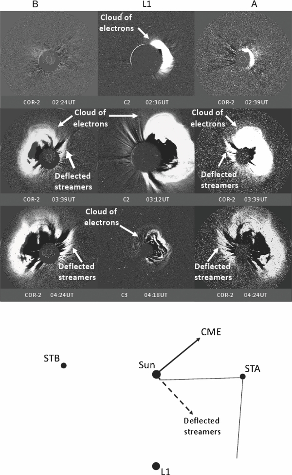
Figure 1. Running-difference images of the 2011 March 21 CME obtained by COR-2B (left-hand column), C2/C3 (middle column), and COR-2A (right-hand column). The "cloud of electrons" and deflected streamers are labeled.
Download figure:
Standard image High-resolution imageThe top and middle rows present coronagraphic observations obtained near 02:30 UT and 3:30 UT, respectively. A major difference between these two times is the entrance in the COR-2 fields of view of the CME off one limb of the Sun and the perturbed streamer rays off the opposite limb. The streamers appear like thin bands (or "stalks") of brightness variation extending nearly radially outward. The CME that erupted off one limb could somehow push streamers observed off the opposite limb. Another noticeable change is the appearance of a layer of brightness variation surrounding the CME, which we will refer to as a "cloud of electrons." The cloud of electrons extends over a wide range of position angles (P.A.s) and over greater heliocentric radial distances than the CME. Previous studies have associated this cloud with the formation of a compression region around the CME (Vourlidas et al. 2003; Ontiveros & Vourlidas 2009). Similarly, perturbed streamers have been related to the effect of pressure variations passing through these otherwise stationary coronal features (e.g., Sheeley et al. 2000). Combined analysis of white-light images and numerical simulations showed evidence that the leading edges of these clouds may be the location of an outflowing shock (e.g., Vourlidas et al. 2003; Manchester et al. 2008). The cloud of electrons, as well as the pushed streamers enclosed in that cloud, could be the white-light signatures of the pressure variations launched by the sudden expansion of the CME. A third noticeable effect is the impacts of energetic protons between 02:39 UT and 03:39 UT in COR-2A images that are absent in COR-2B. Movies of C2/C3 running-difference images also reveal impacts of energetic protons at SOHO by 04:18 UT.
Figure 2 presents observations of the lower corona made in EUV and white light by SECCHI-A between 02:15 UT and 03:54 UT. The first perturbations of the lower corona imaged in 195 Å by the EUVI occur between 02:05 and 02:10 UT. Flaring activity is seen in an active region located W131°N22°, shortly after, by 02:15 UT, a clear EUV bubble forms. As the bubble expands it perturbs the corona over an area that increases roughly circularly around the source region. By 02:40 UT, the EUV bubble extends out into the COR-1 field of view as a CME. The leading edge of this CME appears as a thin white and black band, this band is traditionally termed the "pileup." Part of this pileup results from the white-light integration of plasma located on the curved surface of erupting transients (Chen et al. 1997; Thernisien et al. 2006). This pileup can grow as additional coronal material gets swept up by the erupting CME (e.g., Hundhausen 1972; see review by Thernisien et al. 2011). Consistent with past studies, we refer to the region located below this pileup as the "driver gas" (e.g., Hundhausen 1972). This driver gas may be a magnetic flux rope (Chen et al. 1997), although evidence for the presence of a flux rope is not clear by simply looking at these images. In any case, this event is not an obvious flux rope CME, unlike the gradually accelerating ones that often have a clear croissant-shaped aspect (e.g., Thernisien et al. 2011). By 02:55 UT, the CME has expanded eastward and streamers that are located off the east limb are perturbed. In the COR-2 field of view, the pileup is not as clear since we have somewhat saturated the contrast to increase the visibility of the cloud of electrons that surrounds the CME in the upper corona.

Figure 2. Running-difference images made by EUVI-A (top row), COR-1A (middle row), and COR-2A (bottom row). The EUV observations were made at 195 Å. The EUV bubble and wave, the pileup of electrons located on the surface of the driver gas, as well as the deflected streamers and the cloud of electrons are labeled. The kinematic analysis shown in Figure 6 was based on the measurements taken along three lines of constant position angles shown in the bottom left-hand panel.
Download figure:
Standard image High-resolution imageThe central axis of the driver gas remained aligned with the P.A. of the source region (P.A. ∼300°) suggesting that the CME underwent little latitudinal deflection during its outward propagation. By assuming that the CME propagated radially outward from the flaring site (as suggested by the shape and location of the bubble seen in Figure 2), we can convert projected speeds measured along the central axis of the CME (P.A. ∼300°) to true radial speeds. Based on COR-2A observations, the inferred radial speed is roughly 1100 km s−1, a more precise analysis of the kinematic variations is given later in the paper. The COR-1A observations show that the nose of the CME flattened and its sides expanded significantly in latitude as it propagated outward. Using the 5 minute cadence COR-1A images, we estimated the changing P.A. of the sides of the CME and obtained a lateral expansion speed of ∼450 km s−1 between 02:15 UT and 02:40 UT. The bubble forms behind the limb as viewed from L1 and is occulted by the limb before 02:15 UT during the early expansion phase of the CME. Unlike other CME expansions tracked by the Solar Dynamics Observatory (SDO) on the visible disk (Olmedo et al. 2012; Rouillard et al. 2012), we could not measure the high expansion speeds that are likely to have occurred before 02:15 UT.
Figure 3 presents a summary of radio measurements obtained in the decimetric range by the Bruny Island Radio Spectrometer (BIRS) (a) and in the kilometric range made by STA (b), STB (c), and the Wind (d) spacecraft. A Type II radio burst was detected by BIRS between 02:17 and 02:37 UT. Decimetric Type II bursts are caused by coronal shocks, while kilometric Type II bursts are caused by shocks propagating in the upper corona and interplanetary medium. The CME onset shown in Figure 2 was the only erupting transient observed on the Sun at the time and we associate this Type II burst to a coronal shock forming during the eruption of this fast and wide CME. The Type II onset occurs when the CME enters the COR-1A field of view and undergoes its lateral expansion (the CME has by 02:40 UT reached an oval shape in Figure 2 due to this expansion). As we shall see, the solar particle release (SPR) time inferred from energetic particle measurements at STA occurs during this Type II radio burst. A kilometric Type II burst is observed by the radiometers on STA and Wind and is clearest in the STA data. All kilometric Type II bursts observed by ISEE-3 were known to be associated with CMEs and interplanetary shocks (e.g., Cane et al. 1982). These bursts are one of the clearest signatures of shocks moving in the interplanetary medium. The kilometric Type II burst is primarily measured at STA because it is a front-side halo for STA.

Figure 3. Radio measurements made in the decimetric range by the Bruny Island Radio Spectrometer (BIRS) (a) and in the kilometric range made by STA (b), STB (c), and Wind (d). The red dashed line marks the time of the first disturbance observed in EUVI (∼02:15 UT). The white and black dashed lines mark the SPR time along STA (SPR-A) and along L1 magnetic field lines (SPR-L1) calculated from the velocity dispersion analysis presented in Section 3. The times of decimetric and kilometric Type II bursts are also shown.
Download figure:
Standard image High-resolution imageThe radio measurements made in the kilometric range (b,c,d) reveal the presence of complex Type III bursts. These Type III bursts are not observed in the BIRS data and are extremely weak in the Learmonth data (02:25–02:32 UT over the 25–45 MHz range). The source of non-thermal electrons for complex Type III bursts has been debated extensively: these electrons may originate in flare blast waves (Cane et al. 1981), flares (Kundu & Stone 1984; Klein 1995; Bougeret et al. 1998), or CME-driven shocks (Gopalswamy et al. 2000; Klassen et al. 2002). This debate is beyond the scope of this paper, we simply note that the near absence of decimetric Type III bursts observable at Earth could be related to the occultation of the source of non-thermal electrons since both the flare and the CME originate behind the west limb (or ∼W132°) as viewed from Earth. As pointed out by Gopalswamy et al. (2003) and MacDowall et al. (2003), large SEP events and fast and wide CMEs, such as the one studied here, are always associated with complex Type III bursts.
2.2. The Lateral Expansion of the CME
In this section, we argue that combined EUVI and COR-1 observations can be used to track not only the latitudinal expansion of the CME, but also its eastward (i.e., longitudinal) expansion. The nature of EUV "waves" is still largely debated; they have been interpreted as fast-mode waves (Dere et al. 1997; Thompson 1999; Wang 2000; Wu et al. 2001; Patsourakos & Vourlidas 2009), slow-mode shock waves and vortices behind the piston-driven shock (Wang et al. 2009), successive stretching of the closed field lines overlying the erupting flux rope of the CME (Chen et al. 2002), or the result of successive magnetic reconnection driven by the expanding flanks of CMEs (Attrill et al. 2007a, 2007b). It is also debated whether these waves are driven by a piston, or are freely propagating, and whether they may be launched and/or driven by flares, CMEs, or small-scale ejecta. Past studies using low-cadence ultraviolet images (>12 minutes) showed that EUV waves are correlated with CMEs rather than flares (Plunkett et al. 1998; Cliver et al. 1999; Biesecker et al. 2002) and they tend to have average speeds less than 400 km s−1 (Warmuth et al. 2004; Wills-Davey & Attrill 2009). However, these modest average speeds are unlikely to be the whole story in that 90% of decimetric Type II bursts occur during EUV waves (Klassen et al. 2000). More recent stereoscopic analyses demonstrate a close relation between the location of EUV waves and the compression wave developing on the flanks of CMEs (e.g., Veronig et al. 2009; Patsourakos & Vourlidas 2009). Other case studies by Cheng et al. (2012) and Rouillard et al. (2012) of EUV waves observed with high-cadence images (12 s) taken by the Atmospheric Imaging Assembly (AIA; Lemen et al. 2011) on board the SDO (Lemen et al. 2011) provide evidence that the EUV disturbances are unlikely to be simply propagating fast-mode waves during the first few minutes associated with the initial expansion of the CME since their speeds (>900 km s−1) are in excess of coronal fast-mode speeds (∼400–500 km s−1). It is likely that the wave is initially strongly "driven" by compression during the first few minutes of the CME expansion. The lateral expansion of the CME ceases within minutes and AIA observations show that the waves carry on propagating on the solar surface more slowly, at close to the fast-mode speeds (∼400–500 km s−1; Patsourakos et al. 2009; Kozarev et al. 2011). During this phase the waves may reflect and refract at coronal structures situated on their path (coronal holes, see: Gopalswamy et al. 2009) in analogous ways to blast waves associated with nuclear explosions (the under water "Baker shot" launched in the Bikini atoll is a good example of refracted and reflected blast waves: Glasstone & Dolan 1977). Patsourakos & Vourlidas (2009) and other recent comprehensive analyses of the link between the EUV wave and the disrupted white-light corona by Rouillard et al. (2012) suggest that the EUV wave tracks the region on the solar surface disrupted by compression waves launched by the CME.
Figure 4 presents three EUV running-difference images combined with COR-1 base-difference images and one EUV running-difference image combined with both COR-1 and COR-2 base-difference images (bottom right-hand panel). Base-difference images are obtained by subtracting a background image computed from images taken before the CME eruption. White-light emission due to the more stable background corona (such as streamers) is therefore removed in these base-difference images, thereby allowing a detailed tracking of the lateral expansion of the CME. All three composite images occur during the decimetric Type II burst when a shock has already formed. These images show that the leading edge of the EUV disturbance is located at the leading edge of the laterally expanding CME, or more specifically the pileup ahead of the driver gas. This EUV disturbance is observed clearly until the CME's lateral expansion ceases between 02:30 and 02:38 UT. After 02:38 UT, the latitudinal and longitudinal extent of the CME is fixed, and the wave continues to propagate parallel to the solar surface, slowly devolving into a broad and less coherent structure that becomes harder to locate. A dashed black line and a black arrow mark the location of the wave in Figure 4 at 02:54 UT. By that time the wave has practically disappeared but has also reached the base of the pushed streamers that become suddenly visible in the running-difference images (see Figure 2). These streamers are engulfed in the cloud of electrons of which the extent is derived from the corresponding running-difference image shown in Figure 2 (at 02:54 UT).

Figure 4. Combined COR-1A and EUVI-A images showing the relation between the propagating EUV disturbance tracked in the lower corona in 195 Å and the CME expanding in the upper corona in the COR-1A field of view at 02:20, 02:30, and 02:38 UT. Black dashed lines and thick white arrows mark the extent of the EUV wave. Bottom right-hand panel: combined EUVI-A, COR-1A, and COR-2A images at 02:54 UT. The thin white arrows shown in the COR-1/2A field of view mark the larger extent of the cloud of electrons surrounding the CME. The limits of this cloud were determined from the sharp drop in coronal brightness observed on its surface in the corresponding running-difference image (bottom left-hand panel of Figure 2).
Download figure:
Standard image High-resolution imageThe clearest and most reliable tracking of the wave can be made between 02:10 and 02:30–02:38 UT and along a latitudinal band centered at 55° where the EUV signal appears strongest. Before 02:30 UT, the EUV wave and the outer edges of the "pileup" observed in white light move together and have consequently similar speeds parallel to the solar surface. A crude measure of the wave speed is made by assuming that the wave is propagating along a constant height of 1.12 R☉ (Patsourakos et al. 2009), we obtained an average speed of ∼430 km s−1 between 02:10 and 02:30 UT, which drops below 300 km s−1 between 02:30 and 02:45 UT. After 02:30 UT, speed measurements of this EUV disturbance were generally difficult to accomplish (even with the use of "J-maps" extracted on the solar disk, see, e.g., Rouillard et al. 2012), due to the broad and more diffuse nature of the wave.
The result of tracking the EUV wave in the corona is plotted in Figure 5 as a series of white contour lines superposed on a Carrington map. The map is constructed by assembling (central) meridional strips of EUVI measurements made at 195 Å over a Carrington rotation period. The positions of the wave measured in individual EUV frames such as Figure 4 (black arrows) are marked by white crosses. The white lines are computed from these positions and by assuming that the wave has propagated uniformly in all directions such that each contour marks the locus of points on the solar surface that are at equidistance from the origin of the wave (the flaring site at W132°N22°). Based on these observations and those presented in other studies (e.g., Patsourakos & Vourlidas 2009), we hypothesize that the wave tracks the extent in latitude and longitude of the high pressure variations developing around the expanding CME and that these white lines may represent the latitudinal and longitudinal extent of an expanding coronal shock. In the following sections, we test this hypothesis by analyzing the temporal and longitudinal properties of the associated SEP event detected at L1 and at STA.

Figure 5. Top panel: a Carrington map of EUV observations made in the 195 Å emission line. The distance between the EUV leading edge along heliographic latitude 55° (black arrows in Figure 4) and the source region of the CME was measured directly from EUV images. The white contours show the extent of the EUV disturbance assuming that the wave is expanding uniformly in all directions. The footpoints of magnetic field lines connected to STA, L1, and STB are shown as black/white circles and were calculated assuming Parker spiral theory. Bottom panel: a GONG magnetogram in Carrington map format. Overlaid onto this map are the contours of the propagating EUV disturbance and the locations of coronal holes (dashed green, dashed positive, red, negative) calculated from a PFSS model. The connection between the various coronal holes and the ecliptic plane is shown as green and red lines.
Download figure:
Standard image High-resolution imageUntil 02:30 UT, the contour lines are confined to Carrington longitudes to 0°–100°. Soon after, the effects of the expanding compression region can be detected in the longitudinal band 330°–360°. The disappearance of the wave after 02:45 UT occurs when the streamers are deflected in COR-1A (02:55 UT), particularly in COR-2A (after 02:54 UT; see Figures 1 and 2). Perturbations at the base of these streamers are also observed at around ∼03:00 UT at Carrington latitude 55° and longitude 300°–310° in the 193 Å emission line by the AIA on board SDO.
The three black and white circles overplotted in Figure 5 mark the estimated latitudes and longitudes of the footpoints of interplanetary magnetic field lines connected to the STEREO spacecraft and to the L1 spacecraft. These locations were calculated from a simple application of Parker spiral theory by using the average solar wind speed measured in situ during the onset of the SEP events, studied later in this paper, at STA (∼420 km s−1), STB (∼410 km s−1), and L1 (∼330 km s−1). We note that these estimated locations are in principle valid only beyond the source surface (i.e., >2.5 Rs) since, at this stage, we ignore the complicated distribution of magnetic field lines in the lower corona.
From a simple reading of the map shown in Figure 5, we observe that the EUV wave approaches the magnetic field lines connected to STA between 02:10 and 02:13 UT, L1 between 02:40 and 02:50 UT, and that it never reaches the magnetic field lines connected to STB. Assuming that the wave is the signature of pressure variations and associated shock capable of accelerating particles, we obtain a first explanation as to why energetic protons impact STA but not STB; STB was located on the opposite side of the Sun and its magnetic field lines were connected to a region of the corona that was not significantly affected by the CME-associated compression region.
The images suggest that the EUV wave is initially driven by the laterally expanding flanks of the CME. The wave becomes a more freely propagating disturbance when the CME stops expanding laterally. SEPs could be accelerated during the lateral expansion phase, especially for events where the wave speed exceeds the fast-mode speeds (400–500 km s−1) and could be associated with a shock formation (Rouillard et al. 2012). However, this phase usually lasts 5–10 minutes and the cadence of EUV images was too low during this event to determine the initial speeds accurately. The analysis presented later in this paper provides strong evidence that the CME-driven shock developed around the leading edges of the CME is the primary source of the SEP.
2.3. The Radial Expansion of the CME
The magnetic field lines connected to L1 and STA are rooted near the vicinity of the white-light disturbance induced by the compression region, detected off the east and west limbs of the Sun viewed from STA. It is therefore interesting to study the kinematic properties of these disturbances since they likely track the evolution of the CME shock. The upper two rows of Figure 6 present the measurements of heliocentric radial distance (left-hand panels) and calculated speed (right-hand panels) of the CME tracked in COR-1/2A off the west limb as a function of time and radial distance, respectively. This tracking is made along the central axis of the CME (∼296°; top row) and along the ecliptic plane (∼275°; middle row). The magnetic field lines connected to STA should be rooted along the ecliptic plane (middle row). The white dashed lines plotted in the bottom left-hand panel of Figure 2 show the radial lines associated with these constant P.A.s.

Figure 6. Three kinematic analysis made at different position angles (top: 296°, middle: 275°, bottom: 91° as shown in Figure 2). The radial distance of the leading edge of the cloud of electrons measured along these three position angles is shown in the left-hand panel, the derived radial component of the shock speed is shown in the right-hand panel. The measurements made along lines of constant position angles located in the ecliptic plane and connected to the STA and L1 particle detectors are shown in the middle and bottom panels, respectively. The functional forms that model the speed variations best are third-order polynomial fits (top and middle panels) and a decaying exponential for the bottom panel. Note that the CME-driven compression region is tracked over much longer radial distances in the bottom panels since the HI-1/2A running-difference images can be used.
Download figure:
Standard image High-resolution imageAssuming that the CME propagates radially outward from the flaring site, we can transform sky-plane distances to true heliocentric radial distances. The derived radial speeds (along P.A. = 296°) are shown in Figure 6(b) as a function of radial difference and show that the CME accelerated slowly in the COR-1 field of view and reached speeds of ∼1200 km s−1, before decelerating back to 1100 km s−1. The evolution of the southern flank of the CME (along P.A. ∼275°) is very different with a speed increasing from 1000 km s−1 to 1400 km s−1 at 12 R☉ and then decelerating rapidly back to ∼1150 km s−1 when it exits the COR-2 field of view (∼22 R☉). Third-order polynomial fits accurately reproduce the kinematic variations seen accurately.
To derive the kinematic variations of the pushed streamers shown in the bottom row of Figure 6, we show in Figure 7 a section (off the east limb of the Sun as viewed from STA) of a straight COR-2A image (a), and with the previous frame subtracted from it (b). STA observes the streamers mostly face-on as a thin latitudinally extensive sheet of plasma (Figure 7(a)), this streamer is made of individual stalks that are often seen in the face-on views of streamers (Thernisien & Howard 2006). Like in previous CME events seen in LASCO, the passage of the shock wave is made visible, like "amber waves of grain," in this field of coronal rays (Sheeley et al. 2000). A white arrow marks the location of one of these stalks in Figure 7(a). These stalks appear as white–black bands in the running-difference image suggesting that they are displaced by the pressure variations developing around the CME. These perturbed structures then propagate out into the heliosphere where they are imaged by the HIs. An HI-1A running-difference image of these outflowing structures is shown in Figure 7(c).

Figure 7. Left: a background-subtracted COR-2A image taken of the east limb of the Sun. Middle: the corresponding running-difference image; right: an HI-1A image of the deflected streamer tracked in the heliosphere. Arrows point to single streamer stalk convected out with the compression wave of the CME.
Download figure:
Standard image High-resolution imageThe trajectories of these pushed streamers are of particular interest to the present analysis since the occurrence of their perturbations is closely timed with the arrival of the EUV wave at their base. They also propagate in the HIs and therefore their true direction of propagation and speed can be derived accurately using the techniques that we developed in previous studies of heliospheric images (see Rouillard et al. 2009, 2010; Sheeley & Rouillard 2010). We could track each of the sub-structures associated with the pushed streamers by using our J-mapping technique. J-maps are built by extracting strips of pixels from each image and plotting each strip vertically with time (Sheeley et al. 1999). These maps allow us to track the elongation variation of plasma structures with great accuracy. The elongation variation (α(t)) of a density front moving radially outward with a constant speed (Vr) along a solar radial at an angle (δ) out of the sky plane is then related by
where D is the distance away from the Sun. The first step is to assume that when the plasma structure has reached a certain distance away from the Sun (here 60 R☉), it moves radially outward at a constant speed. A functional form is then used to fit the acceleration/deceleration in the lower corona (here we use a decaying exponential function). The result of this analysis along a P.A. ∼91° (near the ecliptic plane) is shown in the bottom panels of Figure 6. The perturbed streamer ray moves outward with an initial speed of 920 km s−1 and at an angle of δ ∼ 54 5. It is decelerating rapidly (average deceleration of −6 km s−2) between 0 and 60 R☉ to reach ∼500 km s−1. This analysis was repeated along different latitudes and we found that the initial speeds of these streamer stalks were generally higher (∼1100–1300 km s−1) at higher latitudes (P.A. ∼60°–80°) than in the near-ecliptic latitudes (∼800–900 km s−1). Similar latitudinal gradients were observed by Sheeley et al. (2000) in their kinematic analysis of perturbed streamers using LASCO images, although their analysis was limited by projection effects since only the LASCO images could be used at the time. The Carrington coordinates of the origin of the various deflected streamer stalks seen in Figure 7 were determined using the derived three-dimensional trajectories and were plotted onto the Carrington map shown in Figure 5 (top panel) as white diamonds. They all originated from a highly convoluted part of the heliospheric neutral line (see Figure 5, bottom panel). The derived launch times of these deflected structures were 02:45–02:55 UT, i.e., when the pressure variations reach the base of these streamers.
Figure 8 summarizes the findings in this section with a schematic of the ecliptic plane viewed from solar north (left-hand column) and the meridional plane containing the footpoints of magnetic field lines connected to STA (right-hand column) for three different times. The eruption of the CME is associated with a strong disturbance propagating in the EUV corona. During a first "lateral expansion phase" of the CME, the white-light extension (i.e., in COR-1) of the EUV wave is the pileup surrounding the driver gas (a,b). The EUV wave develops near the outer edges of the laterally expanding driver gas and retains its shape until the driver gas ceases expanding (b,e). In a second phase (hereafter 02:30 UT), the pileup and the wave separate rapidly and the wave devolves into a less coherent structure (c,f). By ∼02:55 UT, the COR-1 coronagraphs detect the strong perturbation of streamers off the west limb of the Sun as viewed from STA (c). Although the base-difference images (COR-2A) suggest a remote influence of the driver gas erupting primarily off the west limb (Figure 4(d)), running-difference images show that these streamers are enclosed in a cloud of electrons that extends spatially well beyond the regions reached by the driver gas or even the pileup located on its surface (Figure 4). This cloud of electrons is transported outward with the CME, and shows the full extent of the region perturbed by the pressure variations that have been launched by the CME eruption. The initial speeds of the pushed streamers (900–1200 km s−1) are generally lower than the leading edge of the CME measured off the opposite limb (1100–1500 km s−1). From simple Parker spiral theory, we determined that the pushed streamers are magnetically connected to L1 and that the leading edge of the CME is magnetically connected to STA. From this schematic, we speculate that the shock geometry along magnetic field lines connected to L1 is likely to be quasi-perpendicular because these field lines are connected to the flanks of the compression regions. The magnetic field lines connected to STA are initially connected to the southernmost edge of the shock (the CME erupts from N22°), also giving initially a quasi-perpendicular geometry, but the shock geometry is likely to rapidly become quasi-parallel as the CME propagates in the corona. This geometry is drawn in top right-hand panel which shows a view of the meridional plane connected to STA. As the CME expands, the magnetic field lines will increasingly intersect the surface of the CME and the driven shock orthogonally to form a quasi-parallel shock. Of course this only a schematic and a more detailed numerical simulation (e.g., Sandroos & Vanio 2007, 2009) should be carried out to test this basic picture. We have already run a standard potential field source surface calculation, with superposed in the meridional plane connected to STA, the location and shape of the surface of the CME shock observed in white light which confirms this basic picture. More events such as the March 21 event will be analyzed in a similar fashion and reported in a further study.

Figure 8. Schematic of the ecliptic plane viewed from solar north (left-hand column) and the meridional plane containing the footpoints of magnetic field lines connected to STA (right-hand column) for three different times. The expanding driver gas, the pileup of electrons, the EUV wave, the pushed streamers, and the shock are represented in this diagram. The magnetic field lines connected to STA and L1 are shown.
Download figure:
Standard image High-resolution image3. THE TIMING OF THE SEP EVENTS
Figure 9 compares the first arrival of SEPs at STA (top panel) and at L1 (bottom panel), using 1 minute averaged intensities of ∼0.7–3 MeV electrons and two high-energy proton channels, at ∼35–40 and at ∼60–100 MeV. The STA measurements came from the High Energy Telescope (HET), part of the IMPACT package on STA (Luhmann et al. 2008). The electron measurements at L1 were provided by the Electron Proton Helium Instrument (EPHIN) part of the Suprathermal and Energetic Particle Analyzer (COSTEP; Müller-Mellin et al. 1995) on board SOHO. The Energetic and Relativistic Nuclei and Electrons (ERNE) instrument (Torsti et al. 1995), also on SOHO, provided the L1 proton measurements shown here. Velocity dispersion in the first arrival of particles is evident at both locations. The onset of the electron flux at SOHO occurs around 03:034 ± 3 minutes or some ∼30 minutes after the increase in electron flux measured at STA. The ∼60–100 MeV and ∼35–40 MeV protons measured at L1 started to increase at ∼40 and ∼50 minutes, respectively, after the commensurate proton onsets measured at STA. As shown below, these delays require that the first release of particles onto the Sun–L1 field line occurred well after the first release of particles onto the Sun–STA field line.

Figure 9. Top panel: the 1 minute averaged intensity of 0.7–2.8 MeV electrons (blue), 35.5–40.5 MeV protons (red), and 60–100 MeV protons (green) measured by the HET instrument on board STA. Bottom panel: the 1 minute averaged intensities of electrons and protons in nearly the same energy bins as measured by the EPHIN and ERNE instruments on SOHO. Note that proton intensities have been multiplied by a factor of 10 for ease of comparison. Vertical lines mark the estimated onset times of the MeV electron flux increases at both spacecraft. The pre-event electron background is similar at both spacecraft, but the proton background at SOHO/ERNE is much larger than at STEREO-A/HET. This difference may be instrumental, at least in part. Comparison of these particular energy channels at that time shows that the proton/electron ratio is ∼50 times larger at STEREO-A than at SOHO.
Download figure:
Standard image High-resolution imageIn Figure 10, the top panels present the solar wind speed measured in situ by the PLASTIC instrument (Galvin et al. 2008) on STA (left) and by the Solar Wind Experiment (SWE; Ogilvie et al. 1995) on Wind at L1 (right). The bottom panels show the corresponding two-day history of proton intensities at STA and at L1 in six energy bins between ∼1 and ∼100 MeV. The SEP event observed at L1 and at STA can be classified as long-lasting "gradual SEPs" (Reames 1999) at both L1 and STA, with the event measured at L1 being much weaker than at STA. The flux of high-energy protons (60–100 MeV) at STA rises and falls over a 12 hr period but the flux of lower-energy protons (with energies <4 MeV) rises steadily until 18 UT on March 22 when an interplanetary shock passes by STA. This interplanetary shock can be seen in top left panel of Figure 10 as the discontinuous change in speed from 420 to 770 km s−1. No shock was measured in situ at L1 during this SEP event. Our simple analysis of the lateral expansion of the compression region (Figure 5) suggested that in situ signatures of the CME shock should be detected at STA but not at L1 or STB, consistent with the solar wind data. By using minimum variance analysis directly over the shock surface and shock mass flux conservation equation, we determined that the shock speed was 630 km s−1, this shock speed stands between the shock speeds measured off the STA west limb along the southern flank of the CME (1100 km s−1 by 5 UT on March 21) and the speeds measured off the L1 west limb along the pushed streamers (500 km s−1 by 12 UT on March 22).

Figure 10. Top panels: solar-wind proton speed measurements from PLASTIC-A at STA (left) and from SWE on Wind at L1 (right). Bottom panels: proton intensities measured in six energy bands spanning ∼1–100 MeV from the HET, LET, and SIT instruments on STA (left) and from ERNE on SOHO at L1 (right). The proton intensities from STA and from SOHO are 1 minute and 5 minute averages, respectively. The proton energy bins were chosen so as to be nearly the same on both spacecraft. The arrival of the interplanetary shock at STA is marked. Data gaps are apparent in the Wind and SOHO data.
Download figure:
Standard image High-resolution imageFigures 11(a) and (b) present two velocity dispersion analyses based on the arrival times of particles with different energies at STA and L1, respectively. A velocity dispersion analysis can be obtained by plotting the onset times of particle flux increases versus the reciprocal of the relativistic beta value (β−1 = (v/c)−1) for different particle energies (Krucker et al. 1999; Tylka et al. 2003). A linear fit on such a scatter plot determines the initial solar particle release (SPR) time, as the intercept, and the path length followed by the particles between the Sun and L1, as the slope. The particle onsets measured by the STA HET instruments were sharp and a well-defined linear relation is found between the arrival time and speed of the particles (cyan and black diamonds). The particle data (protons, helium-4, oxygen, and iron) measured by the Low Energy Telescope (LET) instruments also shows a similar velocity dispersion. A linear fit to HET and LET data points shown in Figure 11 gives a path length of 1.45 ± 0.05 AU and an estimated release time of 02:19 ± 00:03 UT at the Sun. For comparison with the time lags on images, the ∼8 minutes required for electromagnetic radiation to reach STA are added so that the release time becomes 02:27 ± 00:03 UT.

Figure 11. Top panel: a velocity dispersion analysis based on the measurements of the onset of electrons, light (protons), and heavy ions (oxygen, 4helium, and iron) at STA. Bottom panel: a velocity dispersion analysis based on the measurements of the onset of electrons and protons by EPHIN and the onset of protons by ERNE.
Download figure:
Standard image High-resolution imageThe velocity dispersion analysis derived from measurements of energetic particles at L1 is shown in Figure 11(b) and uses electron and proton data from the EPHIN instrument and proton data from the ERNE instrument. Unfortunately, no data were recorded by the Wind spacecraft during the SEP onset and we could therefore not use 4He particle data for their velocity dispersion analysis. The derived path length was 1.81 ± 0.14 AU with an SPR time of 02:57 ± 00:05 UT (again an 8 minute time lag was added to compare the electromagnetic observations with the estimated SPR times). The two SPR times derived by these velocity dispersion analyses are shown on the radiospectrograms as white dashed lines in Figure 3 (top panel) and black dashed lines in Figure 3 (across the three bottom panels). The two SPR times occur during the decimetric and kilometric Type II bursts. The Appendix provides additional information on the velocity dispersion analysis at STA and its reliability by using a transport model of SEPs. In particular, it was found that the SPR time obtained from the velocity dispersion analysis derived from STA data is accurate to within 2 minutes.
As noted in Section 2, the compression wave reaches the longitudes of the footpoints of magnetic field lines connected to STA and L1 at ∼02:15 UT and ∼02:50 UT, respectively. We therefore find evidence that the delayed onset of the SEP events measured here at different heliocentric longitudes during the same solar storm could be associated with the time required by the driver gas to expand over a wide range of longitudes. Cliver et al. (2005) studied a far side (W180°) CME event with speed of 1500 km s−1, that erupted on 2001 August 15–16 and that was associated with 400 MeV protons at L1. Although they lacked the imaging capabilities to study the expanding CME and its shock in the first hour after eruption, they also found an SEP onset at L1 within 40 minutes of the eruption, which they interpreted to the expansion time of the CME shock. Our study supports such an interpretation, for a well-observed CME event using unprecedented multi-point observations of the far side of the Sun.
4. COMPOSITION AND SPECTRAL PROPERTIES OF THE SEP EVENT
SEP elemental and isotopic abundance ratios provide valuable information on the origins of these particles. Particularly useful in this regard are the 3He/4He and Fe/O ratios. An analysis of the 3He/4He ratio, using data from the Ultra Low Energy Isotope Spectrometer (ULEIS; Mason et al. 1998) on ACE, gave an event-integrated value of 3He/4He ∼ (10 ± 7) × 10−4 at 0.5–2.0 MeV nucleon−1. To within errors, this result is consistent with the average solar wind value of (4.08 ± 0.25) × 10−4 (Gloeckler & Geiss 1998). SIT-A is not able to detect 3He at such low levels. The mass histogram from SIT-A at comparable energies indicates only that 3He/4He < 0.1, a weak upper limit that is not very informative.
Figure 12 presents the event-integrated Fe/O ratio as a function of energy, as derived from measurements made by ACE/Solar Isotope Spectrometer (SIS), Wind/EPACT/LEMT, and ACE/ULEIS at L1. Below a few MeV nucleon−1, these values are comparable to the average gradual SEP value of 0.134 ± 0.004 (Reames 1995). With increasing energy, however, the Fe/O value rises, approaching (but not attaining) the impulsive SEP average of 1.078 ± 0.046 (Reames 1995). This pattern of energy dependence was observed in many events in Cycle 23 (Tylka et al. 2002; Tylka 2005). Tylka & Lee (2006) showed how this behavior could be understood quantitatively in a simplified analytical model of a shock that evolves from quasi-perpendicular to quasi-parallel as it moves through the corona, operating on seed particles that include suprathermals from preceding flares (or other reconnection activity). This proposed scenario was subsequently examined and modeled with numerical simulations of a simplified coronal shock (Sandroos & Vanio 2007, 2009). The CME-imaging in this event points toward such a scenario, in that an initially quasi-perpendicular shock is likely to develop near the base of the pushed streamers, on the far eastern flank of the CME as viewed from STA (Figure 8). However, we have no direct information on the other requirement of the Tylka & Lee scenario, namely, the presence in the corona of suprathermals with impulsive-SEP-like composition.
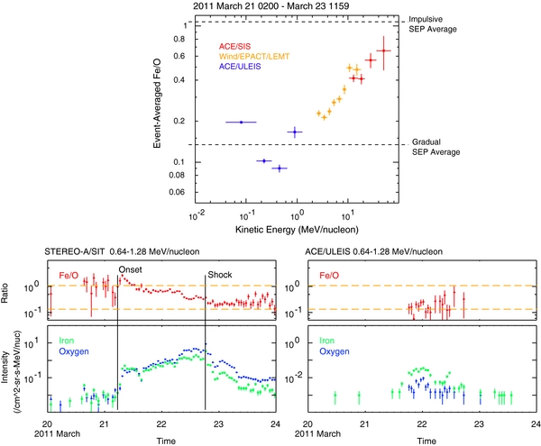
Figure 12. Hourly averaged Fe/O ratio (top) and Fe and O intensities (bottom) from STA/SIT (left panels) and from ACE/ULEIS (right panels) at L1 at 0.64–1.28 MeV nucleon−1 (right panels). The vertical lines in the STA panel show the expected time of first arrival for the highest energy particles in these bins, based on the velocity dispersion analyses in Figure 11, and the time of shock arrival. Dashed horizontal lines show the average SEP Fe/O ratio for gradual and impulsive events, at 0.134 and 1.078, respectively, from Reames (1995). At STA, the 21 March event appears to have been preceded by one or more impulsive SEP events.
Download figure:
Standard image High-resolution imageAs shown in Figure 8, it is expected that lateral expansion will cause the shock's first contact with the Sun-STA field line also to be quasi-perpendicular. Accordingly, it would not be surprising to find Fe/O similarly increasing with energy at STA. The LET and HET instruments on STA measure Fe and O above ∼4 MeV nucleon−1. As shown in Figure 12, onsets were identified in the LET oxygen and iron channels. However, LET and HET Fe and O measurements are not yet available for the rest of the event, when virtually all of the fluence is collected.
It has also been suggested that enhanced Fe/O at high energies is the signature of ions accelerated in the concomitant flare (Cane et al. 2003), similar to the heavy-ion enhancements seen in impulsive SEP events at lower energies. In this scenario, there is no need for any subsequent interaction between flare-accelerated particles and the shock to attain the observed energies. In the concomitant flare scenario, it might be surprising to find enhanced high-energy Fe/O at L1 but not at STA. If high-energy Fe/O were indeed present at STA, this scenario would require that particles from the flare dominate the production of heavy ions above ∼30–50 MeV nucleon−1 over more than 90 deg of heliolongitude.
The ULEIS instrument on ACE and the Suprathermal Ion Telescope (SIT) on STA allow for comparison of Fe/O ratios below ∼2 MeV nucleon−1. Fe and O measurements from these instruments at 0.64–1.28 MeV nucleon−1 are shown in the bottom panels of Figure 12. At STA, Fe/O is initially enhanced and decays over the duration of the event, reaching roughly nominal values only after the shock passage. This evolution is most likely a transport effect, with the extended duration of the decay reflecting the role of proton-amplified waves. At L1, the observed Fe/O values are at roughly the average SEP value for gradual events throughout the event. Transport-induced-enhanced Fe/O at the start of the event may have been undetectable at L1 because of the smaller intensities. (Note the different vertical-axis scales for the STA and ACE intensities.)
Figure 13 compares average proton intensities measured by instruments located at L1 on board ACE (EPAM), SOHO (ERNE, EPHIN), and Wind (LEMT) and by instruments on board STA (SEPT-A, SIT-A, LET-A, and HET-A) during the first 21 hr of the SEP event (March 21, 3–24 UT). The SEPT-A and EPAM instruments measure ion intensities but protons are the most common ions measured near 1 AU and therefore these ion measurements are good proxies for the proton intensities. The time interval considered for this spectrum does not contain the shock passage at STA (i.e., March 22 at 18 UT). As we can see the spectra are very different at STA and L1, the proton intensities are 100 times higher at 10 MeV, 50 times higher at 60–100 MeV but only 10 times higher at 1 MeV. The ERNE and GOES instruments detected protons with energies exceeding 400 MeV, the Payload for Antimatter Matter Exploration and Light-nuclei Astrophysics detected protons reaching 600 MeV near 1 AU (M. Casolino 2011, private communication); however, no ground-level events (GLEs) were observed by Earth-based neutron monitors, which suggests GeV protons were probably extremely low during this event. Unfortunately, the highest energy channel on STA is 60–100 MeV. Considering how hard the spectrum is at STA and the fact that the flux of 60–100 MeV protons is 50 times higher than at L1, it is possible that a significant flux of GeV protons was generated along the magnetic field lines connected to STA.

Figure 13. Proton spectra averaged over the first 21 hr of the SEP event at STA (SEPT-A ions, SIT-A, LET-A, HET-A) and at L1 (EPAM ions, LEMT, EPHIN, ERNE, GOES). In accumulating the spectrum at L1, gaps in the SOHO/ERNE timelines were filled by using ∼2 and ∼20 MeV proton measurements from Wind/EPACT as templates.
Download figure:
Standard image High-resolution imageGoing from high to low energies, the flux of protons increases monotonically from 100 MeV to 3 MeV and then decreases slightly, forming a plateau between 0.1 and 3 MeV. This effect has been seen in other intense SEP events. Reames (1990) showed that few MeV protons accelerated in large shock events frequently exhibit a flat intensity–time profile. This effect was studied further by Reames & Ng (2010), who argue that an energy spectral plateau may occur when numerous outwardly streaming protons amplify resonant Alfvén waves that scatter lower-energy protons and reduce their anti-sunward streaming. The streaming limit of MeV protons is not expected when there are few high-energy protons to make waves. This is the case at L1 where the SEP event is much weaker (Figure 13). The streaming limit of MeV protons is not observed for weaker SEP events. This is the case at L1 in Figure 13 where the SEP event is much weaker.
The dip in proton flux near 3× 10⁻¹ MeV nucleon−1 measured by STA is attributed in the paper to the effect of self-generated waves preventing these lower-energy particles from escaping the region upstream of the shock. The simulated spectra that we obtained from the simulation shown in the Appendix show a similar dip at 3× 10⁻¹ MeV nucleon−1 and is a property of spectra attributed to the effect of self-generated waves (Reames & Ng 2010). The origin of the flux increase observed in the STA spectra for decreasing energies (around 3× 10⁻¹ MeV nucleon−1) beyond the dip is less clear. It could be attributed to background effects. This topic will be addressed in detail in a forthcoming paper by C. K. Ng et al. (2012, in preparation).
5. EFFECT OF THE LONGITUDINAL VARIABILITY OF THE SHOCK SPEED
Particle kinetic energy gain in diffusive shock acceleration theory arises from the coupling of the energetic particles to the compression at the shock via scattering from the magnetic irregularities on either side. This theory predicts that the peak intensities of SEPs should be related to the speed of CMEs since the speed of the driver gas relative to the ambient plasma will set, to a large extent, the level of plasma compression and therefore dictate the value of the shock compression ratio (see, e.g., Lario et al. 1998). Indeed, studies of protons between ten of keV to ∼100 MeV detected at interplanetary shocks measured in situ show that at a given energy, the particle flux enhancement increases with the shock speed along the upstream magnetic field and with the shock compression ratio. For this reason, the highest intensities at a given energy are usually achieved near the inferred nose of the interplanetary shock (Cane et al. 1988). Additional supporting evidence for the shock-diffusive acceleration was presented in the form of a relation between CME shock speed inferred from white-light images and the peak intensity of energetic protons measured at 2 and at 20 MeV (Reames 1999; Kahler 2001). According to this relation and the shock speed analysis presented in this paper, we would expect STA to measure much stronger proton fluxes than the L1 spacecraft. Figure 14 reproduces the scatter plot of proton peak intensity versus CME speed given as Figure 1 in Kahler (2001). The relation is quite broad as noted by Kahler. Our analysis provides multi-point measurements of the CME shock front at different longitudes, allowing us to compare shock speeds and SEP intensities in the same event but at different longitudes.

Figure 14. Reproduced here, is Figure 1 of Kahler (2001), showing peak proton intensity as a function of CME speed for 2 MeV protons (left) and 20 MeV protons (right). Also shown are the comparison of proton peaks and averages during the first plateau reached during the SEP events measured at STA (red squares) and L1 (hollow red squares) vs. peaks and averages of the shock speeds measured by SECCHI-A during the corresponding time intervals. Horizontal bars crossing the squares show the range in CME speeds observed during the time interval considered.
Download figure:
Standard image High-resolution imageThe spatial and temporal variability of shock speeds measured during the single CME event analyzed here suggests that at least part of the large scatter seen in Figure 14 could result from poorly measured CME shock speeds inferred from the single viewpoints offered by the SOHO and SOLWIND coronagraphs. The maximum CME speeds measured by LASCO were used for the events shown in Kahler (2001), but these speeds may not be representative of conditions along the magnetic field lines connected to the proton events measured in situ. As seen in Figure 10, the proton flux is time variable with a sharp flux increase at all energies occurring during the SEP onset followed by a period when proton fluxes reach more stable flux values or a peak "plateau." For the proton channel 20.8–23.8 MeV (HET-A, Figure 10), the peak proton flux measured during the first 12 hr of the event was ∼36 ± 0.7 protons (cm2 sr s MeV)−1. To determine the CME shock speed, we refer to Figure 6 (middle panels) and take the peak CME speed reached soon after CME eruption (∼1400 km s−1). We repeated the analysis for protons measured by SIT (Figure 10) in the 1.8–2.9 MeV range. The results are plotted as red squares in Figure 14.
The same analysis was carried out for particle measurements along magnetic field lines connected to L1 and compared to the shock speeds measured with the deflected streamers (bottom right-hand panel of Figure 6). The peak speed occurs at onset and was ∼900 km s−1, much lower than the speed measurements made along magnetic field lines connected to STA. This combination of ACE/SOHO proton measurements with SECCHI-A derived speed measurements are shown as hollow squares.
These new points are very close to the relations inferred by Reames (1999) and Kahler (2001) and inside the inherent scatter. The points inferred here suggest a steeper dependence of the proton flux as a function of CME speed than derived by Reames (1999). Of course similar analysis done for more events is necessary to assess whether a steeper dependence is a general property. Our analysis is also limited by the use of white-light images, our analysis of shock speeds assumed that the shock normal was pointing anti-sunward, this is probably not the case since the shock normal is likely to have an off radial component, particularly near the flanks of the CME shock in the vicinity of the deflected streamers. A future study could attempt to derive shock speeds using full numerical MHD simulations such as those presented in Rouillard et al. (2011) but for the inner corona.
6. DISCUSSION AND CONCLUSION
The lateral expansion of the CME across latitudes and longitudes could be measured with the 5 minute cadence COR-1 images combined with 3 minute cadence EUVI images. We found that an EUV wave tracked closely the expansion of the plasma pileup surrounding the driver gas of the CME with an average speed of 450 km s−1 using the low image cadence offered by STEREO. The lateral expansion of the pileup ceased when its flanks encountered the edge of a streamer which is clearly deflected in the upper corona. The speeds of these deflected coronal rays were in excess of 900 km s−1 and decelerated rapidly to less 500 km s−1 by 50 R☉.
The SEP was triggered by activity on the far side of the Sun as viewed from Earth (W132°), yet proton detectors located in the vicinity of Earth measured protons with energies exceeding 100 MeV. The coronal footpoints of magnetic field lines connected to STA and L1 were separated by 90° at the time. We found that the lateral expansion required 30 minutes to cross this longitudinal extent. Velocity dispersion analyses revealed that the SPR time at L1 was delayed by 30 minutes with respect to STA.
The mapping of coronal disturbances presented in this paper shows that the lateral expansion of the CME and its driven shocks can influence the heliosphere over 90° (the separation between STA and L1), however we only considered the expansion of the compression wave eastward from the point of origin. STB observations of the east limb of the corona show that the compression wave expanded westward as well, if one assumes a symmetrical expansion from the point of origin, then the compression wave may have reached a longitudinal extent of 180° already in the upper corona.
In light of the wide range of observations presented in this study, it is important to state precisely what the results of the paper are.
- 1.It shows that the lateral expansion of fast and wide CME events can last 30–40 minutes and is related to the expansion of EUV waves in the lower corona confirming previous studies by Patsourakos & Vourlidas (2009) and Veronig et al. (2009). In the present study, the EUV disturbance initially tracks the flank of the laterally expanding driver gas.
- 2.It provides an interpretation of the delayed onset of a solar particle event measured by widely separated spacecraft in terms of the lateral expansion of a CME and the associated CME-driven compression region propagating in the lower corona. This was suggested in the study of Krucker et al. (1999) who investigated, using low-cadence EUV wave measurements from EIT, the electron events that were released up to half an hour later than the onset of the Type III burst.
- 3.
- 4.It also demonstrates that a single CME be associated with vastly varying shock speeds along different latitudes and longitudes in the lower corona (as suggested before in Sheeley et al. 2000).
The acceleration processes that produce SEPs in large events (with energies exceeding 400–500 MeV) is still an area of active debate. The particle energies measured during the March 21 SEP event exceeded 400 MeV at L1 and, since the event was stronger at STA than at L1, particle energies likely also exceeded 400 MeV at STA. The present study provides an interpretation of the timing and longitudinal range of the SEP event in terms of the three-dimensional evolution of CME-driven pressure variations. We relate the strong and weak particle fluxes observed at STA and L1, respectively, with the different speeds, strengths, and perhaps geometries of the shocks crossing their respective magnetic field lines. Supporting this scenario, we present relations between SEP intensity and the speed of launched coronal disturbances.
However, this study did not assess the alternative scenario that these SEPs may originate in the solar flare that occurs during the eruption of the CME. If particles were accelerated in the solar flare, a fraction of these particles would have to remain trapped on closed magnetic field lines (perhaps those of the CME) until the particles diffused from the flaring site to the open magnetic field lines connected to L1. Particle trapping would occur if "bottle breaking" overcame collisional losses for 30 minutes or more. The few MeV electrons and 200–300 MeV protons would suddenly have access to open field lines rooted in the deflected helmet streamers. Some particles would stream out into the interplanetary medium (to be measured at L1), other particles would propagate toward the chromosphere and generate X-ray or gamma-ray emissions. A future study could investigate whether hard X-rays or gamma rays were detected by the sensitive detectors on the Reuven Ramaty High Energy Solar Spectroscopic Imager and other space-based gamma-ray detectors during this event.
In a future theoretical study, we will also investigate the origin of the different spectral properties measured at L1 and STA in terms of the longitudinal variability of the shock (speed, compression ratio, and geometry) and the effect of high-energy particles altering the "waves/turbulence," located upstream of the shock (streaming limit). We are confident that more detailed case studies involving a wider range of CME/flares and particle detector configurations will allow us to decide which acceleration mechanism is more likely.
We thank Dennis Haggerty for providing the EPAM ion data plotted in Figure 13. We thank Dr. Valtonen for making the ERNE data available online. The SECCHI images were obtained from the World Data Center, Chilton, UK and the Naval Research Laboratory, Washington, DC, USA. We thank Yi-Ming Wang and Judith Lean for their continual support. We also acknowledge constructive exchanges with Ed Cliver and Raúl Gómez Herrero. The STEREO SECCHI data are produced by a consortium of RAL (UK), NRL (USA), LMSAL (USA), GSFC (USA), MPS (Germany), CSL (Belgium), IOTA (France), and IAS (France). The ACE data were obtained from the ACE science center. The Wind data were obtained from the Space Physics Data Facility. The work of C.M.S.C. and R.A.M. on ACE data was partly funded by the NASA contract NNX08AI11G. The Caltech subcontract SA2715-26309 was funded with NASA contract NAS5-0313 (UC Berkeley). The work of A.P.R. was partly funded by NASA contracts NNX11AD40G-45527 and NNXIOAT06G and that of C.K.N. was partially supported by NASA grant NNX09AU98G. NASA contract SA4889-26309 from University of Berkeley (STEREO SIT) and NASA grant NMX07AN45G permitted the preparation and calibration of the ULEIS and SIT data. A.J.T. was supported in part by NASA grant NNH09AK79I. The NRL employees acknowledge support from the Office of Naval Research and NASA.
APPENDIX: RELIABILITY OF SEP VELOCITY DISPERSION ANALYSES
SEP velocity dispersion analyses, like those shown in Figure 11, have been used in numerous studies (Lin et al. 1981; Reames et al. 1985; Krucker et al. 1999; Krucker & Lin 2000; Tylka et al. 2003; Reames 2009a, 2009b). When applied to two, unusually large and well-measured impulsive SEP events, it was found that the SPR times coincided with the peaks in the hard X-ray emissions to within 1–2 minute uncertainty (Tylka et al. 2003). For gradual events, SPR times occurred after the peak intensities of solar gamma rays (Tylka et al. 2003), as well as after reported onsets of Type II emissions (Reames 2009a, 2009b). SPR times in gradual SEP events generally correspond to times when the leading edge of the associated CME is at ∼2–6 solar radii from Sun center. In studies of GLEs, Reames (2009a, 2009b) also found that the heights at which SPR release occurred were ordered with source-region longitude in a way that is qualitatively consistent with particle acceleration by an expanding shock wave.
The 2011 March 21 event, at least as observed at STA, is well suited for the analysis of velocity dispersion. As shown in Figure 15 (discussed in more detail below), pre-event backgrounds—both instrumental and otherwise—were low, and the proton intensities increased rapidly at onset.

Figure 15. Observed onset in 1 minute averaged proton intensities (blue) from the High Energy Telescope (HET) on STEREO-A in six different energy bins and the simulated onset in these same energy bins from the Ng et al. (2003) transport model. The model gives intensities in absolute units, so there is no arbitrary adjustment of normalizations. In some panels, the data show a few particles that register before the steep rise of the onset. These may be the result of small levels of contamination from protons with energies above the stated maximum energy of the bin.
Download figure:
Standard image High-resolution imageHowever, some theoretical studies (Lintunen & Vainio 2004; Saiz et al. 2005) have shown that the results of velocity dispersion analyses can be misleading in some circumstances. To assess this concern for the present study, we have combined our SPR analysis with a detailed numerical simulation of the STEREO observations. The simulation is based on the Ng et al. (2003) focused transport SEP model. This model includes the effects of proton-amplified wave growth, which gives rise to dynamic scattering conditions that depend on time, location, and rigidity. As discussed by Reames (2009a), this evolution in the scattering conditions means that the first-arriving particles experience less scattering than those that arrive later, something that was not taken into account in previous theoretical studies of SEP velocity dispersion. The transport model also includes the full pitch-angle distribution, so that protons of a given energy can interact with a spectrum of Alfvén waves and vice versa. Finally, because the wave growth is a nonlinear process, this model necessarily deals with intensities in absolute units. As a result, we can apply to the simulation the same onset-identification criteria used in the data analysis. Additional details about the transport model and its application to this particular event will be given elsewhere (C. K. Ng et al. 2012, in preparation).
In this study, we used a threshold intensity of 0.005 p (cm2 sr s MeV)−1 for protons in the HET-A energy range (∼13–100 MeV) and 0.01 p (cm2 sr s MeV)−1 for protons in the LET-A energy range (∼4–10 MeV). In the simulation, we set the SPR time at 02:20 Solar Time (ST), as suggested by the fit in Figure 11. We then varied the length of the magnetic field line until we found a value that gave a velocity dispersion plot whose fit parameters were close to those found in the data. For a physical path length of 1.34 AU, the simulated velocity dispersion shown in Figure 16 gave a fitted distance of 1.45 AU, matching the value found from the data. The difference between the nominal Parker spiral length (1.14 AU for a solar wind speed of 450 km s−1) and 1.34 AU is presumably due to field-line meandering (Pei et al. 2006). The difference between the apparent distance (1.45 AU) and the input path length (1.34 AU), on the other hand, reflects the effects of the comparatively small amount of scattering experienced by the first-arriving particles. In addition, the SPR time deduced from the simulated velocity dispersion is later than the actual input SPR time by less than 3 minutes.

Figure 16. Velocity dispersion analysis of the simulated proton data for STEREO-A, analogous to the top panel of Figure 11, which shows the actual data.
Download figure:
Standard image High-resolution image
Figure 15 shows six examples of the proton time–intensity profile at onset, using 1 minute averaged intensities from STEREO and from the simulation. In these comparisons, the simulated time-dependent proton spectra have been integrated over the same energy bins as the data. Although the simulations do not reproduce the fine structure of the onsets, the overall agreement in the onset times, the slopes of the intensity rise at onset, and the attained intensity values are generally very good. Based on the good agreement in these comparisons, we believe that the simulated velocity dispersion provides a realistic assessment of the reliability of the velocity dispersion analysis of the data.
We note that the present version of the transport model injects the energetic protons at ∼8 Rs, rather than the ∼3 Rs value indicated by Figure 6. Ions with energies of 2 and 100 MeV nucleon−1 take ∼2.8 and ∼0.4 minutes, respectively, to traverse 5 Rs, so the higher injection altitude has negligible effect on the dispersion analysis. Also, the transport calculations assume a purely radial magnetic field, which, compared with the Parker spiral, slightly overestimates the strength of the focusing that occurs beyond ∼0.5 AU. Improvement of these features of the transport model will be addressed in future work. Nevertheless, the current version is adequate to address the reliability of the velocity dispersion analysis. Specifically, the fitted path length is longer than the actual length of the interplanetary magnetic field line by ∼10% due to scattering, and the inferred SPR time is no more than ∼3 minutes late.
Finally, it should be noted that the HET and LET instruments have limited viewing angles out of the ecliptic plane (latitude ±275). The magnetic field measured in situ during the onset of the SEP was fluctuating with elevation angles reaching 35°–40°. The derived SPR measured by HET and LET may therefore be slightly delayed compared with the true onset despite the very sharp particle increases measured during the SEP onset. Future work could investigate numerically the pitch-angle distribution for this event and attempt to refine the SPR times further by applying some form of time correction. We note that an earlier derived SPR time along STA magnetic field line might improve the agreement with the release time of particles estimated from the location of the EUV wave.