


ABSTRACT
We characterize the dust in NGC 628 and NGC 6946, two nearby spiral galaxies in the KINGFISH sample. With data from 3.6 μm to 500 μm, dust models are strongly constrained. Using the Draine & Li dust model (amorphous silicate and carbonaceous grains), for each pixel in each galaxy we estimate (1) dust mass surface density, (2) dust mass fraction contributed by polycyclic aromatic hydrocarbons, (3) distribution of starlight intensities heating the dust, (4) total infrared (IR) luminosity emitted by the dust, and (5) IR luminosity originating in regions with high starlight intensity. We obtain maps for the dust properties, which trace the spiral structure of the galaxies. The dust models successfully reproduce the observed global and resolved spectral energy distributions (SEDs). The overall dust/H mass ratio is estimated to be 0.0082 ± 0.0017 for NGC 628, and 0.0063 ± 0.0009 for NGC 6946, consistent with what is expected for galaxies of near-solar metallicity. Our derived dust masses are larger (by up to a factor of three) than estimates based on single-temperature modified blackbody fits. We show that the SED fits are significantly improved if the starlight intensity distribution includes a (single intensity) "delta function" component. We find no evidence for significant masses of cold dust (T ≲ 12 K). Discrepancies between PACS and MIPS photometry in both low and high surface brightness areas result in large uncertainties when the modeling is done at PACS resolutions, in which case SPIRE, MIPS70, and MIPS160 data cannot be used. We recommend against attempting to model dust at the angular resolution of PACS.
Export citation and abstract BibTeX RIS
1. INTRODUCTION
Interstellar dust affects the appearance of galaxies, by attenuating short-wavelength radiation from stars and ionized gas, and contributing IR, submillimeter, mm, and microwave emission (for a review, see Draine 2003). Dust is also an important agent in the fluid dynamics, chemistry, heating, cooling, and even ionization balance in some interstellar regions, with a major role in the process of star formation. Despite the importance of dust, determination of the physical properties of interstellar dust grains has been a challenging task—even the overall amount of dust in other galaxies has often been very uncertain.
Many previous studies have used far-infrared photometry to estimate the dust properties of galaxies. For example, Draine et al. (2007) used global photometry of 65 galaxies in the "Spitzer Infrared Nearby Galaxies Survey" (SINGS) galaxies to estimate the total dust mass and polycyclic aromatic hydrocarbon (PAH) abundance in each galaxy, and to characterize the intensity of the starlight heating the dust. For most of these galaxies the photometry extended only to 160 μm, although ground-based global photometry at 850 μm was also available for 17 of the 65 galaxies.18 Muñoz-Mateos et al. (2009) used images of the SINGS galaxies to examine the radial distribution of the dust surface density. Sandstrom et al. (2010) studied the PAHs in the Small Magellanic Cloud (SMC) on a pixel-by-pixel basis with a very similar dust model as the present work. Very recently, Totani et al. (2011) used global photometry in six bands—9, 18, 65, 90, 140, and 160 μm—to estimate dust masses for a sample of more than 1600 galaxies in the Akari All Sky Survey. In the present work, we develop state-of-the-art image processing and dust modeling techniques aiming to reliably determine the dust properties in resolved studies.
The present study makes use of combined imaging by the Spitzer Space Telescope and Herschel Space Observatory, covering wavelengths from 3.6 μm to 500 μm, to produce well-resolved maps of the dust in two nearby galaxies. The present study is focused on two well-resolved spiral galaxies, NGC 628 and NGC 6946, as examples to illustrate the methodology. Subsequent work (G. Aniano et al. 2012, in preparation) will extend this analysis to all 61 galaxies in the KINGFISH sample (Kennicutt et al. 2011).
The paper is organized as follows. In Section 2 we discuss the data sources. Background subtraction and data processing are discussed in Section 3. The dust model is summarized in Section 4, and the fitting procedure is described in Section 5. Results for NGC 628 and NGC 6946 are given in Section 6. The sensitivity of the derived parameters to the set of cameras used to constrain the dust models is explored in Section 7, where we compare dust mass estimates obtained at high spatial resolution (without using Multiband Imaging Photometer (MIPS)160 or the longest wavelength Spectral and Photometric Imaging (SPIRE) bands) with estimates made at lower spatial resolution (using all the cameras available). We also investigate the reliability of the photometry by comparing MIPS70 and MIPS160 images with PACS70 and PACS160 images. In Section 8 we compare dust mass estimates based on spatially resolved images with dust mass estimates based on global photometry, as would apply to distant, unresolved galaxies. The "goodness of fit" of different dust models is discussed in Section 9. The principal results are discussed in Section 10 and summarized in Section 11.
Appendices A–D describe the method for image segmentation (i.e., galaxy and background recognition), background subtraction, estimation of photometric uncertainties in the images, and estimation of dust modeling uncertainties. Appendix E is a comparison of Photodetector Array Camera and Spectrometer for Herschel (PACS) and Multiband Imaging Photometer for Spitzer (MIPS) photometry.
2. OBSERVATIONS AND DATA REDUCTION
NGC 628 and NGC 6946 are part of the SINGS galaxy sample (Kennicutt et al. 2003), and were imaged by the Spitzer Space Telescope (Werner et al. 2004). A large subset of the SINGS galaxies are also included in the Herschel Space Observatory Open Time Key Project KINGFISH (Kennicutt et al. 2011) and were observed with the Herschel Space Observatory (Pilbratt et al. 2010).
We will use "camera" to identify each optical configuration of the observing instruments, i.e., each different channel or filter arrangement of the instruments will be referred to as different "camera." With this nomenclature, each "camera" has a characteristic optical resolution, spectral response, and point-spread function (PSF).19 We will refer to the Infrared Array Camera (IRAC), MIPS, PACS, and SPIRE cameras using their nominal wavelengths in microns: IRAC3.6, IRAC4.5, IRAC5.8, IRAC8.0, MIPS24, MIPS70, MIPS160, PACS70, PACS100, PACS160, SPIRE250, SPIRE350, and SPIRE500. For our standard modeling, the PACS and SPIRE data were reduced by HIPE followed by Scanamorphos (see Section 2.2.1 for details). In Appendix E, and Table 6, where we compare PACS data with and without Scanamorphos processing, we use PACS(H)70, PACS(H)100, and PACS(H)160 to denote PACS data that were processed by the HIPE pipeline only.
Table 1 summarizes the optical resolution of the cameras.
Table 1. Image Resolutions
| FWHMa | 50% Powera | Final Grid | Compatible | |
|---|---|---|---|---|
| Camera | ('') | Diameter ('') | Pixelb ('') | Camerasc |
| IRAC3.6 | 1.90 | 2.38 | ... | Not used as a final-map PSF |
| IRAC4.5 | 1.81 | 2.48 | ... | Not used as a final-map PSF |
| IRAC5.8 | 2.11 | 3.94 | ... | Not used as a final-map PSF |
| IRAC8.0 | 2.82 | 4.42 | ... | Not used as a final-map PSF |
| PACS70 | 5.67 | 8.46 | ... | Not used as a final-map PSF |
| MIPS24 | 6.43 | 9.86 | ... | Not used as a final-map PSF |
| PACS100 | 7.04 | 9.74 | ... | Not used as a final-map PSF |
| PACS160 | 11.2 | 15.3 | 5.0 | IRAC; MIPS24; PACS |
| SPIRE250 | 18.2 | 20.4 | 8.0 | IRAC; MIPS24; PACS; SPIRE250 |
| MIPS70 | 18.7 | 28.8 | 10.0 | IRAC; MIPS24,70; PACS; SPIRE250 |
| SPIRE350 | 24.9 | 26.8 | 10.0 | IRAC; MIPS24,70; PACS; SPIRE250,350 |
| SPIRE500 | 36.1 | 39.0 | 15.0 | IRAC; MIPS24,70; PACS; SPIRE |
| MIPS160 | 38.8 | 58.0 | 16.0 | IRAC; MIPS; PACS; SPIRE |
Notes. aValues from Aniano et al. (2011) for the circularized PSFs. bThe pixel size in the final-map grids is chosen to Nyquist sample the PSFs. cOther cameras that can be convolved into the camera PSF (see the text for details).
Download table as: ASCIITypeset image
2.1. Spitzer
The IRAC and the MIPS cameras on the Spitzer Space Telescope were used to observe all 75 galaxies in the SINGS sample, including NGC 628 and NGC 6946, following the observing strategy described by Kennicutt et al. (2003). Spectroscopic observations of selected regions were also obtained, although not used in the current study. G. Aniano et al. (2012, in preparation, hereafter ARD12) use the spectroscopic observations of selected regions to further constrain the dust modeling.
2.1.1. IRAC
IRAC (Fazio et al. 2004) imaged the galaxies in four bands, centered at 3.6 μm, 4.5 μm, 5.8 μm, and 8.0 μm. The images were processed by the SINGS Fifth Data Delivery pipeline.20 The IRAC images are calibrated for point sources. Photometry of extended sources requires so-called "aperture corrections." We multiply the intensities in each pixel by the asymptotic (infinite radii) value of the aperture correction (i.e., the aperture correction corresponding to an infinite radius aperture). We use the factors 0.91, 0.94, 0.66, and 0.74 for the 3.6 μm, 4.5 μm, 5.8 μm, and 8.0 μm bands, respectively, as described in the IRAC Instrument Handbook (V2.0.1).21
2.1.2. MIPS
Imaging with MIPS (Rieke et al. 2004) was carried out following the observing strategy described in Kennicutt et al. (2003). The data were reduced using the LVL (Local Volume Legacy) project pipeline.22 A correction for nonlinearities in the MIPS70 camera was applied by the team, as described by Dale et al. (2009) and Gordon et al. (2011).
2.2. Herschel
The PACS and the SPIRE cameras on the Herschel Space Observatory are being used to observe the 61 galaxies in the KINGFISH sample, in particular NGC 628 and NGC 6946, following the observing strategy described by Kennicutt et al. (2011). The maps were designed to cover a region out to ≳ 1.5 times the optical radius Ropt, with good signal to noise (S/N) and redundancy. The depth of the PACS images at 70 μm and 160 μm is less than that of MIPS, but the higher resolution of PACS is able to better single out compact star-forming regions.
2.2.1. PACS
NGC 628 and NGC 6946 were observed with the PACS instrument on Herschel (Poglitsch et al. 2010) on 2010 January 28 (NGC 628) and March 10 (NGC 6946), using the "Scan Map" observation mode. The PACS images were first reduced to "level 1" (flux-calibrated brightness time series, with attached sky coordinates) using HIPE (Ott 2010) version 5.0.0, and maps ("level 2") were created using the Scanamorphos data reduction pipeline (Roussel 2012), version 16.9. This reduction strategy includes the latest PACS calibration available (Müller et al. 2011), and aims to preserve the low surface brightness diffuse emission.
Additionally, PACS data were reduced completely (i.e., to "level 2") using HIPE. We used HIPE version 5.0.0, and further divide the fluxes by 1.119, 1.151, and 1.174 for the cameras PACS70, PACS100, and PACS160, respectively, to account for the latest calibration of the cameras. Both PACS data reduction strategies present strong discrepancies with the corresponding MIPS photometry, as is discussed in Appendix F. The HIPE pipeline removes a large fraction of the flux in the low surface brightness areas, and in our work it was only used for comparison, i.e., we found (Appendix F) that the Scanamorphos pipeline is more reliable, and we only employ the Scanamorphos reductions when PACS data are used in the dust modeling.
2.2.2. SPIRE
The two galaxies were observed with the SPIRE instrument (Griffin et al. 2010) on 2009 December 31 (NGC 6946) and 2010 January 18 (NGC 628). The data were first reduced to "level 1" using HIPE version spire-8.0.3287, followed by Scanamorphos version 17.0.23 The assumed beam sizes are 435.7, 773.5, and 1634.6 arcsec2 for SPIRE250, SPIRE350, and SPIRE500, respectively. Additionally, we excluded discrepant bolometers from the map and adjusted the pointing to match the MIPS24 map. Data reduction details can be found in Kennicutt et al. (2011).
2.3. Atomic and Molecular Gas
NGC 628 and NGC 6946 are in The H i Nearby Galaxy Survey (THINGS; Walter et al. 2008), with ∼6'' resolution H i 21 cm imaging by the NRAO Very Large Array. The H i 21 cm emission is assumed to be optically thin, in which case the H i surface density is directly proportional to the 21 cm line intensity.
The CO J = 2 → 1 transition was observed with ∼13'' angular resolution by the HERA CO Line Extragalactic Survey (HERACLES; Leroy et al. 2009) using the HERA multi-pixel receiver on the IRAM 30 m telescope, with estimated uncertainties of ±20%.
As is usual, the H2 mass surface density is taken to be proportional to the CO J = 2 → 1 line intensity. XCO is the ratio of H2 column density to CO J = 1 → 0 intensity integrated over the line profile. In what follows, we define
and we assume a J = 2 → 1/J = 1 → 0 antenna temperature ratio R21 = 0.8 (Leroy et al. 2009).
The conversion factor XCO is uncertain. XCO, 20 ≈ 2 is the value normally adopted for molecular gas in the Milky Way (MW; Dame et al. 2001; Okumura et al. 2009). Planck Collaboration et al. (2011b) found XCO, 20 = 2.54 ± 0.13 for the MW. Draine et al. (2007) found that XCO, 20 ≈ 4 appeared to give the most reasonable dust/H mass ratios for the SINGS galaxy sample. Blitz et al. (2007) found XCO, 20 ≈ 4 to be the best overall value for galaxies in the Local Group. Leroy et al. (2011) found XCO, 20 = 1.2–4.2 for M 31, M 33, and the Large Magellanic Cloud (LMC), and the very high values XCO, 20 = 14 and XCO, 20 = 32 for NGC 6822 and the SMC. In the present work, we take XCO, 20 = 4 ± 1 to be the best overall value for NGC 628 and NGC 6946. In Section 6 (Figure 3) we show the H gas maps and dust/H mass ratio for XCO, 20 = 2, 3, 4.
The H i and H2 masses are added to generate maps of the total H surface density ΣH. Including helium would give Σgas ≈ 1.38 × ΣH, but in our discussion will use ΣH as it is the "observable," avoiding uncertainties in the helium abundance.
3. IMAGE ANALYSIS
Before modeling the spatially resolved spectral energy distributions (SEDs), it is necessary to adjust the images in a number of ways to ensure meaningful results. In the following sections we describe the image analysis steps in detail. These steps include background estimation and subtraction, convolution to a common PSF, and resampling of the convolved images to a common pixel grid. We also correct the final images for missing or bad data in the original images and estimate the uncertainties on the flux in each pixel. The pixel sizes used in the final maps are chosen to Nyquist sample the final-map PSFs.
All camera images are first rotated so that north is up, and then trimmed to a common sky region. We then estimate and remove a background from each image, as described in Appendix B. Following this, we convolve the images to a common PSF, and resample all the images on a common final-map grid. We correct the final images for the bad pixels (or missing data) in the original images, as described in Appendix C. Finally, we use the background pixel dispersion to estimate the pixel flux uncertainties, as described in Appendix D.
3.1. Background Recognition and Subtraction
We use a multistep algorithm to generate a Background Mask, consisting of the area not covered by either the target galaxy or other discrete sources (e.g., recognizable background galaxies or foreground stars). This algorithm is described in detail in Appendix A and avoids overestimating the background in cameras with low S/N.
After the background mask is generated, for each image we estimate the best-fit background "tilted plane," as described in Appendix A. After the final best-fit background "tilted plane" has been found for each camera, it is subtracted from the original images. The background subtraction is performed on each original map independently, using its native pixel grid.
The result is, for each camera, a background-subtracted image with its native pixel grid and PSF. Figures 1 and 2 show the resulting background-subtracted images.
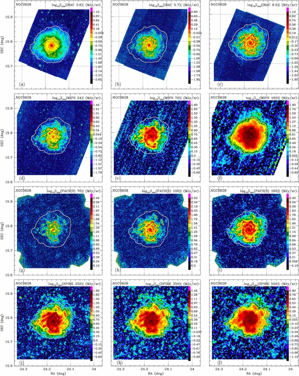
Figure 1. Background-removed images of NGC 628. Top row: IRAC3.6, 5.8, 8.0 (left, middle, and right row, respectively). Second row: MIPS24, 70, 160. Third row: PACS70, 100, 160. Bottom row: SPIRE250, 350, 500. The white contour is the boundary of the galaxy mask, within which the data allow reliable estimation of the dust properties.
Download figure:
Standard image High-resolution image
Figure 2. Same as Figure 1, but for NGC 6946.
Download figure:
Standard image High-resolution image3.2. Convolution to a Common PSF
In order to perform any resolved dust study, it is necessary to convolve all the images to a common PSF. To generate maps with appropriate wavelength coverage to perform the dust modeling, the natural final-map PSFs to use are those of the PACS160, SPIRE250, MIPS70, SPIRE350, SPIRE500, and MIPS160 cameras. For a given final-map PSF, only a subset of cameras may be transformed into it reliably, and we proceed to investigate the most reasonable compatible camera combinations, considering the tradeoff between (1) angular resolution and (2) availability of long-wavelength data to constrain the dust models. After choosing the appropriate PSF for a given set of cameras, we transform all the background-subtracted images to this common PSF using convolution kernels described by Aniano et al. (2011). In Section 6 we will focus on maps generated at three final-map PSFs: PACS160, SPIRE250, and MIPS 160. PACS160 is the PSF with smallest full width at half-maximum (FWHM) that allows use of enough cameras to constrain the dust SED (IRAC, MIPS24, and PACS70, 100, 160). SPIRE250 allows use of the same cameras as PACS160 plus the SPIRE250 camera. Adding the 250 μm constraint produces more reliable maps. The MIPS160 PSF allows inclusion of all the cameras (IRAC, MIPS, PACS, SPIRE), therefore producing the most reliable dust maps; this will be our "gold standard."
The convolution kernels assume that the PSFs can be approximated by rotationally symmetric functions. In general, a convolution kernel will relocate flux in the images to transform them to a desired PSF. Aniano et al. (2011) developed a criterion for camera compatibility, to determine which cameras can be reliably transformed into a given PSF. Essentially, a PSF can be safely transformed into another PSF with similar extended wings provided that the final FWHM is larger than the original. When the extended wings of the two PSFs are dissimilar, the criterion involves quantifying the amount of energy that a kernel should remove from the extended wings of the first PSF, as this power removal is correlated with the risk of introducing artifacts in the convolved image. The performance of the convolution kernels is excellent: for "safe" pairs of PSFs, the discrepancies between the convolved narrower PSF and the broader PSF are smaller than the uncertainties in determining the PSFs themselves.24Arab et al. (2012) implemented a method to construct convolution kernels for non rotationally symmetric PSFs, using the theoretical PSFs for the Herschel cameras. This method relies on the theoretical PSFs, whereas in the present method we are able to use rotational averaging to empirically characterize the extended wings of the actual PSFs measured using observations of saturated point sources. Table 1 lists the resolutions of the cameras, the pixel size in the final-map grids used, and the other cameras that can be used at this resolution.
The CO J = 2 → 1 maps (used to generate the H2 maps) are provided in rotationally symmetric Gaussian PSFs with 13 4 FWHM, which can be safely transformed into all the final-map PSFs used. The original H i maps have non-circular Gaussian PSFs (FWHM = 930 × 1188 for NGC 628, and FWHM = 561 × 604 for NGC 6946). When convolving the H i maps into the final-map resolutions, we will use kernels generated for rotationally symmetric Gaussian PSFs with FWHM =
  and
and  for NGC 628 and NGC 6946, respectively.
3.3. Uncertainty Estimation
For each camera, after the image processing (rotation to R.A.–decl., background subtraction, convolution to a common PSF, and resampling to the final grid) the flux in each final pixel is a (known) linear combination of the flux of (in principle) all the original pixels of the camera. If the statistical properties of the uncertainties in the original pixel fluxes were known, it would be possible to propagate these uncertainties (and their statistical properties) to each final pixel. The original maps oversample the beam, and have artifacts that extend over several pixels, so realistic statistical properties of the uncertainties are difficult to determine. We therefore estimate the uncertainties directly in the final (post-processed) image.
Using the pixels of the background mask (adapted to the final-map grid), we measure the dispersion of the background pixels (which includes noise coming from unresolved undetected background sources, image artifacts, and detector noise) as described in Appendix D. By comparing the MIPS and PACS images, we can also estimate a calibration uncertainty, as described in Appendix D.
4. DUST MODEL
The composition of interstellar dust remains uncertain, but models based on a mixture of amorphous silicate grains and carbonaceous grains have proven successful in reproducing the main observed properties of interstellar dust. We employ the dust model of Draine & Li (2007, hereafter DL07), using "MW" grain size distributions (Weingartner & Draine 2001, hereafter WD01). The DL07 dust model has a mixture of amorphous silicate grains and carbonaceous grains, with a distribution of grain sizes, chosen to reproduce the wavelength dependence of interstellar extinction within a few kpc of the Sun (Weingartner & Draine 2001). The silicate and carbonaceous content of the dust grains was constrained by observations of the gas phase depletions in the interstellar medium (ISM).
The bulk of the dust in the diffuse ISM is heated by a general diffuse radiation field contributed by many stars. However, some dust grains will happen to be located in regions close to luminous stars, such as photodissociation regions (PDRs) near OB stars, where the starlight heating the dust will be much more intense than the diffuse starlight illuminating the bulk of the grains. Since our pixels have a large physical size (≈500 pc side for MIPS160 PSF), we will assume that, in each pixel, there is dust exposed to a distribution of starlight intensities.
4.1. Carbonaceous Grains
The carbonaceous grains are assumed to have the properties of PAH molecules or clusters when the number of carbon atoms per grain NC ≲ 105, but to have the properties of graphite when NC ≫ 105, with an ad hoc smooth transition between the two regimes.
A carbonaceous particle of equivalent radius a is taken to have absorption cross section:
where σPAH (H: C, λ) is the absorption cross section per C for PAH material with given H:C ratio, Cabs (graphite, a, λ) is the absorption cross section calculated for randomly oriented graphite spheres of radius a, and the graphite "weight" is taken to be


where we take the transition radius ac = 0.0050 μm. Carbonaceous grains with a > ac are, therefore, treated as having a graphitic component, with the graphite weight fg → 1 for a ≫ ac. However, with fg = 0.01 for a < ac, even very small PAHs are assumed to have a small continuum opacity underlying the PAH features.
The PAH absorption cross section can be represented as the sum of a number of vibrational features with specified central wavelength, FWHM, and band strength. Li & Draine (2001, hereafter LD01) presented a set of resonance parameters that appeared to be consistent with pre-Spitzer observations. Smith et al. (2007) used the PAHFIT fitting software with the SINGS spectra to improve observational determinations of central wavelengths, shapes, and overall strengths of the PAH emission profiles; DL07 used these results to adjust the LD01 profile parameters. Subsequent modeling of the SINGS nuclear spectra (ARD12) led to some additional small changes in some of the PAH band strengths. In the present study we employ the PAH cross sections from DL07 and ARD12.
Draine & Li (2007) adopted the model put forward by Draine & Lee (1984, hereafter DL84) for the far-infrared properties of graphite. Graphite is a highly anisotropic material, with very different responses for  and
and  , where the
  axis is normal to the "basal plane." DL84 included "free-electron" contributions δ
 f⊥, δf∥ to the dielectric tensor, using a simple Drude model for the free-electron response,
where ω = 2πc/λ, and to allow for size effects the "mean free time" τ is taken to be

where τbulk is the mean free time in bulk material, vF is the Fermi speed, and a is the grain radius.
For  we continue to use the graphite dielectric function from DL84. However, for
  , the DL84 free-electron model for δf∥ resulted in an opacity at λ ≳ 100 μm that gave somewhat more emission than observed in the MW cirrus by Finkbeiner et al. (1999). In addition, the free-electron model used by DL84 for
  produced an opacity peak near 33 μm that does not give a good match to Infrared Spectrograph (IRS) observations of emission from regions where the grains are hot enough to radiate near 33 μm. To broaden the opacity peak, we now take the free-electron contribution for
  to be
to be
with ωp, 1 = 1 × 10¹⁴ s−1, and ωp, 2 = 2 × 10¹⁴ s−1. The τj are obtained from Equation (6) with τbulk, 1 = 3.51 × 10⁻¹⁴ s, τbulk, 2 = 0.88 × 10⁻¹⁴ s. This gives a d.c. electrical conductivity ∑j(ω2p, jτj)/4π = 5.62 × 10¹³ s−1 = 62.5 mho cm−1, within the range reported for high-quality graphite crystals at 300 K [∼1 mho cm−1 (Klein 1962) to ∼200 mho cm−1 (Primak 1956)]. This d.c. conductivity is larger than the value 30 mho cm−1 adopted by DL84; the increased conductivity lowers the FIR emission and brings the overall emission spectrum into better agreement with the observed spectrum from Finkbeiner et al. (1999). We take vF = 3.7 × 10⁶(1 + T/255 K)1/2 cm s−1. The two-component free-electron form of Equation (7) is not intended to have physical significance. It is adopted because it is analytic, satisfies the Kramers–Kronig relations, gives a reasonable value for the d.c. electrical conductivity, and results in an opacity that is less peaked than the original single-component form (5). The resulting graphite opacity varies as λ−2 for λ ≳ 200 μm.
4.2. PAH Abundance qPAH
As discussed above, the PAHs are part of the carbonaceous grain population. The PAH abundance is measured by the parameter qPAH, defined to be the fraction of the total grain mass contributed by PAHs containing NC < 103 C atoms. The PAH size distribution used in the DL07 models extends up to PAH particles containing NC > 105 C atoms (a > 6.0 × 10⁻⁷cm). However, IRAC photometry at 5.8 μm and 8.0 μm is sensitive primarily to PAHs with NC ≲ 103 C atoms, small enough so that single-photon heating can result in significant 8 μm emission (see, e.g., Figure 7 of Draine & Li 2007). For the size distribution in the DL07 models, the mass fraction contributed by PAH particles with NC < 106 is 1.478 qPAH.
WD01 constructed grain size distributions with different values of qPAH that were compatible with the average extinction curve in local diffuse clouds. Such models are possible for qPAH ≲ 0.046, with part of the 2175 Å extinction feature contributed by the PAHs, and part contributed by small graphitic grains. For qPAH ≳ 0.046 the predicted 2175 Å feature from the PAHs alone would be stronger than the average observed 2175 Å feature in local diffuse clouds.25
Nevertheless, because the PAH abundance in other regions could conceivably exceed the value in the local MW, the WD01 dust models have been extended by simply adding PAHs to the qPAH = 0.046 model, with no adjustment to the populations of silicate or larger carbonaceous grains. These models produce stronger emission in the PAH emission features, particularly in the IRAC8.0 band. The models were extended to qPAH = 0.10. The models with qPAH > 0.046 have a 2175 Å feature strength larger than the average value in the local ISM.26 The model set was also extended down to qPAH = 0 (the smallest value of qPAH considered by WD01 was 0.0047). Models were computed in a grid of qPAH = 0, 0.01, 0.02, ... 0.10, and linearly interpolated to a grid with spacing ΔqPAH = 0.001.
4.3. Amorphous Silicate Grains
In the DL84 dust model, the amorphous silicate absorption in the infrared was modeled by a set of damped Lorentz oscillators, resulting in an opacity varying as λ−2 for λ ≫ 25 μm. However, the COBE-FIRAS measurements of the λ > 110 μm emission spectrum of dust at high galactic latitudes (Wright et al. 1991; Reach et al. 1995; Finkbeiner et al. 1999) were not accurately reproduced by the λ−2 opacity of the DL84 graphite–silicate model. Li & Draine (2001) therefore made an ad hoc modification to Im() for amorphous silicate at λ > 250 μm, so that it is no longer a simple power law (with the corresponding changes to Re() required by the Kramers–Kronig relations). The adjustments to Im() were not large—the modified amorphous silicate Im() (Li & Draine 2001) is within ±12% of that for DL84 amorphous silicate for λ < 1100 μm—but these modest adjustments brought the emission spectrum for the dust model into fairly good agreement with observations of the emission spectrum of high-latitude dust (see Figure 9 of Li & Draine 2001). The adopted opacity has no dependence on the grain temperature T.
It is possible that the amorphous silicate opacity may in actuality be T-dependent (Meny et al. 2007), and some authors have argued that this is indicated by observations (Paradis et al. 2010, 2011). The "two-level-system" model of Meny et al. (2007), with the standard parameters recommended by Paradis et al. (2011), has the far-infrared spectral index β ≡ dln κ/dln ν near λ = 500 μm varying from ∼2 to ∼1.3 as T increases from 10K to 50K. However, in the present study we find that the DL07 dust model is able to satisfactorily reproduce the observed spatially resolved SEDs, as well as the global emission. At least for near-solar metallicity galaxies such as NGC 628 and NGC 6946, dust models with T-dependent opacities do not appear to be required.
4.4. Dust Heating
Each dust grain is assumed to be heated by radiation with energy density per unit frequency:

where U is a dimensionless scaling factor and uMMP83ν is the interstellar radiation field estimated by Mathis et al. (1983) for the solar neighborhood. We ignore variations in the spectral shape.
Each pixel in our modeling will be larger than 2 × 10⁴ pc2, so it will contain ISM in a variety of physical environments. A fraction (1 − γ) of the dust mass is assumed to be heated by starlight with a single intensity U = Umin (i.e., heated by a diffuse ISM radiation field), while the remaining fraction γ of the dust mass is exposed to a power-law distribution of starlight intensities between Umin and Umax with dM/dU∝U−α.
The starlight heating intensities are thus characterized by four parameters: γ, Umin, Umax, and α, where the fractional dust mass dMd(U) heated by starlight intensities in (U, U + dU) is
for α ≠ 1, and
for α = 1, where  . More complicated starlight heating distributions could be contemplated, but we find that the simple four-parameter (γ, Umin, Umax, α) model of Equations (9) and (10) appears able to usually provide an acceptable fit to observed SEDs in star-forming galaxies with near-solar metallicities.
Galliano et al (2011) recently claimed that the emission from the LMC can be reproduced using a starlight distribution function that lacks the "delta function" component of Equations (9) and (10), i.e., fixed γ = 1. However, we show in Section 9 that adding the "delta function" component significantly improves the quality of the fit for the pixels in NGC 628 and NGC 6946.
Many authors choose to fit the λ ≳ 70 μm emission using a blackbody Bν(Td) multiplied by a power-law opacity ∝λ−β. The best-fit value of Td is closely related to our heating parameters Umin, γ, α. In a subsequent work (G. Aniano & B. T. Draine 2012, in preparation) we show that Td ≈ 20 U0.15min K, when the DL07 SED is approximated by a blackbody multiplied by a power-law opacity.
Given that there may be significant regional variations in the starlight spectrum, U should be interpreted not as a measure of the starlight energy density, but rather as the ratio of the actual dust heating rate to the heating rate for the MMP83 radiation field.
The fraction of dust luminosity emerging in the PAH features does depend on the spectrum of the starlight heating the dust. Draine (2011a) showed that the fraction of the dust emission appearing at 8 μm increases by a factor of 1.57 as the starlight spectrum is changed from MMP83 to a 20 kK blackbody (cutoff at 13.6 eV). If the actual hν < 13.6 eV starlight spectrum is harder (softer) than the MMP83 spectrum assumed in the models, we will overestimate (underestimate) qPAH.
4.5. Contribution of Direct Starlight
Starlight enters in the dust modeling in two ways: via dust heating (as discussed in Section 4.4) and as a direct starlight component (i.e., direct starlight escaping the observed region). Our main goal in the present work is to study the properties of the dust and the starlight heating the dust, so we adopt a simple model for the direct starlight component. Following Bendo et al. (2006) and Draine et al. (2007), we approximate the λ > 3 μm stellar emission from the galaxy as simply

where Ω⋆ is the solid angle subtended by the stars, Bν is the blackbody function, and T⋆ = 5000 K is a representative photospheric temperature to approximate the integrated stellar emission at λ > 3 μm. The direct starlight contribution is thus adjusted by only the parameter Ω⋆. Direct starlight will only contribute significantly to the IRAC bands, and very marginally to MIPS24. In ARD12 corrections arising from photospheric absorption as well as emission from hot circumstellar dust around asymptotic giant branch stars are studied. These corrections are only important in elliptical galaxies with little ISM, and the results in the present paper would be virtually unchanged if included. We also neglect possible reddening at the wavelengths (λ ⩾ 3.6 μm) in the present study.
Although in principle the direct starlight and heating starlight parameters should be connected, the uncertain and complex distribution of dust and stars within the galaxies make such connection very complex.27 Our simplified treatment of the direct starlight should only be regarded as a way of "removing" the direct starlight component from the near infrared photometry so we can have an estimate of the dust emission.
4.6. Dust Model Emission
For each given set of dust parameters (qPAH, γ, Umin, Umax, α), and the given chemical composition, grain size distribution, and grain properties, the dust emission spectrum is computed from first principles.
First, for each given starlight heating parameter U, the temperature distribution of the dust grains (including the PAH component) is computed as described elsewhere (Draine & Li 2001, 2007). This is performed for a logarithmically spaced grid of 41 U values from 0.01 to 108. From the temperature distribution functions, model spectra are computed and stored. To obtain spectra for intermediate U values, we interpolate.
Second, for each starlight heating distribution, the specific power spectrum per unit dust mass pν(model) is computed. We essentially have two independent heating starlight intensity distributions, the "delta function component" (i.e., the dust exposed to U = Umin) and the "power-law component" (i.e., the dust heated by starlight with Umin < U < Umax). Lastly, each pν(model) is convolved with the various spectral response functions28 to obtain the predicted photometry 〈p(model)〉k for each camera k, with nominal wavelength λk. We construct a library of model emission for a finely sampled grid of parameters (qPAH, Umin, Umax, α) and (qPAH, Umin).
5. DETERMINING THE DUST AND STARLIGHT HEATING PARAMETERS
NGC 628 and NGC 6946 are well resolved, with each galaxy providing many independent pixels, even at MIPS160 resolution. For each pixel j, we find the model of dust and starlight that best reproduces the observed SED, within the modeling scheme described by DL07.
As discussed in Section 4.5, starlight enters the fitting in two ways: via direct starlight in the pixel and by heating the dust. The direct starlight contribution to pixel j is adjusted by varying only the parameter Ω⋆, j. The heating starlight intensity is characterized by four parameters: γj, Umin, j, Umax, j, and αj, where the dust mass dMd heated by starlight intensities in (U, U + dU) is given by Equation (9). For each pixel j we adjust the total dust mass Md, j, the PAH abundance parameter qPAH, j (PAH mass fraction), and the characteristics of the starlight heating the dust in that pixel. If mid-IR photometry is unavailable, one loses the ability to constrain qPAH, but (adopting some arbitrary value of qPAH for the modeling), the dust mass estimation itself would be largely unaffected. Fortunately, we do have mid-IR coverage of our galaxies, so we can obtain full qPAH maps for them. The present modeling assumes the grains to be heated by a standard starlight spectrum (corresponding to the starlight in the local ISM), and to have a fixed balance between PAH neutrals and ions. When fitting to IRAC, MIPS, PACS, and SPIRE photometry, the best-fit value of qPAH is then essentially proportional to the strength of the (nonstellar) IRAC8.0 band power relative to the total IR power.
We will find that γj ≪ 1 in nearly all regions where the dust luminosity surface density  : here, Umin, j is presumed to represent the diffuse ISM, or the counterpart to the "infrared cirrus" component of the galaxy (Low et al. 1984), accounting for the bulk of the dust mass in pixel j. The small fraction γj of the dust mass exposed to starlight intensities U > Umin, j is presumed to correspond primarily to dust in star-forming regions.
The model flux density in camera k is
where 〈F⋆(λ)〉k is the direct contribution of starlight given by Equation (11) convolved with the instrumental response function. The dust model is characterized by {Ω⋆, Md, qPAH, γ, Umin , Umax , α}.
In principle, Umax, j could be treated as an adjustable parameter. Previous work (Draine et al. 2007) has shown that the quality of the global fit to the SED is relatively insensitive to the choice of Umax. We experimented by allowing Umax, j to be fitted29 in the resolved maps, and found that the best value for most of the pixels is Umax, j = 107. In the pixels where the resulting best-fit value is not 107, fixing Umax, j = 107 did not decrease the quality of the fit significantly, i.e., the total χ2 is essentially the same, as shown in Section 9. Allowing Umax to be fitted in the range 103 ⩽ Umax ⩽ 107 or fixing it to Umax = 107 does not produce appreciable changes in the inferred dust masses. We therefore fix Umax, j = 107 in our modeling.
The limits on adjustable parameters are given in Table 2. The allowed range for Umin is determined by the wavelength coverage of the data used in the fit. For the SINGS galaxy sample, it was found that if the photometry extends to λmax = 160 μm, models with Umin ⩾ 0.6 are well constrained. However, if longer wavelength data are available, we allow the possibility of cooler dust, heated by starlight intensities U < 0.6, down to Umin = 0.06 if λmax = 250 μm, and down to Umin = 0.01 if λmax ⩾ 350 μm.
Table 2. Allowed Ranges for Adjustable Parameters
| Parameter | Min | Max | Parameter Grid Used | |
|---|---|---|---|---|
| Ω⋆ | 0 | Ωj | Continuous fit | |
| Md | 0 | ∞ | Continuous fit | |
| qPAH | 0.00 | 0.10 | In steps ΔqPAH = 0.001 | |
| γ | 0.0 | 1.00 | Continuous fit | |
| Umin | 0.7 | 30 | When λmax = 160 μm | Unevenly spaced grida |
| 0.07 | 30 | When λmax = 250 μm | Unevenly spaced grida | |
| 0.01 | 30 | When λmax = 350 μm | Unevenly spaced grida | |
| 0.01 | 30 | When λmax ⩾ 500 μm | Unevenly spaced grida | |
| α | 1.0 | 3.0 | In steps Δα = 0.1 | |
| Umax | 107 | 107 | Not adjusted |
Note. aThe fitting procedure uses pre-calculated spectra for Umin ∈ {0.01, 0.015, 0.01, 0.02, 0.03, 0.05, 0.07, 0.1, 0.15, 0.2, 0.3, 0.4, 0.5, 0.6, 0.7, 0.8, 1.0, 1.2, 1.5, 2.0, 2.5, 3.0, 4.0, 5.0, 6.0, 7.0, 8.0, 10, 12, 15, 20, 25, 30}.
Download table as: ASCIITypeset image
We observe that for a given set of parameters {qPAH, Umin, Umax, α} the model emission is multi-linear in {Ω⋆, Mdust, γ}. This allows us to easily calculate the best values of {Ω⋆, Mdust, γ} for a given parameter set {qPAH, Umin, Umax, α}. Therefore, when looking for the best-fit model in the seven-dimensional model parameter space {Ω⋆, Md, qPAH, γ, Umin Umax, α}, we only need to do a search over the four-dimensional subspace spanned by {qPAH, Umin, Umax, α}. In the case of a fixed Umax, the search is performed over a three-dimensional space spanned by {qPAH, Umin, α}. In any case, for the computed grid of {qPAH, Umin, Umax, α}, the multidimensional search for optimal parameters can be performed by brute force, rather than needing to rely on a nonlinear minimization algorithm.
With Umax fixed, for each pixel j, the model library is used to search for the model parameter vector ξj = {Ω⋆, Md, qPAH, γ, Umin, α} that minimizes
where Fobs, j(λk) is the observed flux density and  is the 1σ uncertainty in the measured flux density for pixel j at wavelength λk (see Appendix D for a detailed discussion on how
  is obtained).30
The above procedure yields "best-fit" estimates for the model parameter vector ξj = {Ω⋆, Md, qPAH, γ, Umin, α} for each pixel j. Each pixel is fitted independently of the remaining pixels in the galaxy. Since the final-map pixel size is chosen to Nyquist sample the final-map PSF, the camera images are smooth on a pixel scale. The fact that we obtain smooth parameter maps is an indication of the stability of the fitting procedure, i.e., even though every pixel is modeled independently of its neighbors, the continuity in the images leads to continuity in the results. The quoted "best-fit" parameter maps arise from fitting the observed flux in each pixel.31
5.1. Properties Derived from the Models
The infrared luminosity Ld, j for the dust model in the pixel j is

where P0(qPAH) (which depends only weakly on qPAH) is the total power radiated per unit dust mass by the model when heated by starlight with intensity U = 1, and  is the mass-weighted mean starlight heating intensity, given by
Star-forming regions have significant starlight power absorbed by dust grains in regions of high starlight intensity, which generally correspond to PDRs. We will refer to the luminosity radiated by dust in regions with U > UPDR as LPDR, given by
We take UPDR = 102 as a plausible cutoff to select dust in high intensity regions (choosing another cutoff value would change only the inferred LPDR, j, leaving all the remaining dust parameters unaltered). We further define fPDR, j as
The region observed is at a distance D from the observer and Ωj is the solid angle of pixel j. For each pixel j, the best-fit model vector {Ω⋆, Md, qPAH, γ, Umin, α}j corresponds to a dust mass surface density:
Similarly, we can compute the infrared luminosity surface density  and the surface density of dust luminosity from regions with U > UPDR,
  , as
, as
The DL07 dust models used here are consistent with the MW ratio of visual extinction to H column, AV/NH = 5.34 × 10⁻²² mag cm2/H, for a dust/H ratio  (see Table 3 of Draine et al. 2007). The dust surface density corresponds to a visual extinction (through the disk):
5.2. Global Quantities
After the resolved (pixel-by-pixel) modeling of the galaxy is performed, we compute a set of global quantities by adding or taking weighted means (denoted as 〈...〉) of the quantities in each individual pixel of the map. The total dust mass Md, tot, total dust luminosity Ld, tot, and total dust luminosity radiated by dust in regions with U > UPDR, Ld, tot, are given by
where the sums extend over all the pixels j that correspond to the target galaxy (see Appendix A for the galaxy segmentation procedure). The dust-mass-weighted PAH mass fraction 〈qPAH〉, and mean starlight intensity  , are given by
The dust mass-weighted minimum starlight intensity 〈Umin〉 is given by
The dust-luminosity-weighted value of fPDR, 〈fPDR〉, is
Alternatively, we can fit the dust model to the global photometry for each galaxy32 (i.e., a single-pixel dust model). The dust parameters obtained from the global-photometry (single-pixel) model fit will be compared to the corresponding resolved modeling global quantities defined in Equations (21)–(24) in Section 8.
Clearly, the emission summed over the map will not correspond to the emission of dust exposed to starlight of the form given by Equations (9) and (10) since different pixels will have different values of Umin, j, γj, and αj. For completeness, we could define the dust mass-weighted mass fraction heated by a power-law (U > Umin) component 〈γ〉 as
and an "effective power-law exponent" 〈α〉, defined as the value that satisfies
Unfortunately, 〈γ〉 and 〈α〉 do not turn out to be useful global quantities, and will, in general, differ significantly from the values obtained from the global-photometry (single-pixel) model fit.
5.3. Parameter Uncertainty Estimates
To estimate uncertainties in the derived dust parameters for each pixel j, we simulate data by adding zero-mean random noise δF(λk)j, r, for r = 1, 2, 3, ..., Nr, to the observed flux F(λk)j in each band, and fit the simulated noisy data. In Appendix D we describe the statistical construction of the sample F(λk)j, r of Nr random realizations. For the fit parameters {a, b, ...} ∈ {Ω⋆, Md, qPAH, γ, Umin, α} we have a set of Nr + 1 values and we calculate the covariance matrix:
where a0, b0 are the best-fit parameter values for the observed fluxes, and ar, br are the best-fit values for the rth random noise realization. For each model parameter a, the 1σ uncertainty is taken to be

Each random noise realization r = 1, 2, ...Nr produces a global quantity via Equations (21)–(24) and (26). We proceed to calculate uncertainties for global quantities using Equations (27) and (28). In Appendix E we describe the details of the parameter uncertainty estimation.
6. RESULTS
We construct dust maps with several different angular resolutions. For a given resolution, one can only use cameras with the PSF FWHM smaller than the reference PSF. In a normal star-forming galaxy, most of the dust mass is at temperatures Td ≈ 15–25 K, with νLν peaking at λ ≈ hc/6kTd ≈ 100–160 μm. Reliable estimates of the dust mass therefore require long-wavelength data, at least out to 160 μm. In the present study we will compare dust models using maps at the resolution of the PACS160 (FWHM = 112), SPIRE250 (FWHM = 182), and MIPS160 (FWHM = 388) cameras. As discussed by Aniano et al. (2011) the MIPS160 PSF cannot be convolved safely into the SPIRE500 PSF (with FWHM = 361). This implies that MIPS160 is the narrowest PSF that can be used if we want to include MIPS160 data into the modeling. A drawback of using the MIPS160 PSF is its extended wings, which can cause power radiated by the bright central regions to contribute significantly to the observed surface brightness of the faint outer regions. However, we will see in Section 7 that this effect does not significantly affect dust mass estimates, and discrepancies between PACS and MIPS photometry make it important to include the MIPS160 camera in the dust modeling.
In order to generate the H surface density maps (used in the dust mass/H mass ratio maps), a value of XCO, 20 needs to be chosen. Figure 3 shows the total H maps (first and third rows) for both galaxies, for XCO, 20 = 2, 3, and 4, convolved to the MIPS160 PSF. Note that the CO maps cover almost all of both galaxy masks, but do not cover the full field of view, leading to the box-like step in the H mass maps.

Figure 3. Row 1: total H surface density for NGC 628 at MIPS160 resolution for XCO, 20 = 2, 3, and 4. Row 2: dust/gas mass ratio derived from the dust map in Figure 4(c), and the gas maps in row 1. Row 3: same as row 1, but for NGC 6946. Row 4: dust/gas mass ratio derived from the dust map in Figure 9(c), and the gas maps in row 3. For NGC 628 the dust/gas maps seem best behaved for XCO, 20 = 4 (Figure 3(f)). For NGC 6946 the dust/gas maps outside the central region also seem best behaved for XCO, 20 = 4 (Figure 3(l)).
Download figure:
Standard image High-resolution imageUsing dust maps based on all of the available photometry (with the MIPS160 PSF—see Figures 4(c) and 9(c) below), Figure 3 shows the dust/H mass ratios for the different values of XCO, 20, for NGC 628 (second row) and NGC 6946 (fourth row). The choice XCO, 20 = 4 gives the smoothest dust/H mass ratios over the galaxies (outside of the central region of NGC 6946, which is further discussed in Section 6.2.1). As discussed in Section 2.3, we take XCO, 20 = 4 for both NGC 628 and NGC 6946.
6.1. NGC 628
6.1.1. Maps of Gas and Dust
NGC 628 (= M 74), at a distance D = 7.2 Mpc, is classified as SAc. With major and minor optical diameters of 10.5 and 9.5 arcmin, it is well resolved even by the MIPS160 camera.
The star formation rate is estimated to be 0.7 ± 0.2 M☉ yr−1 (Calzetti et al. 2010). Two supernovae have been observed in NGC 628: SN 2002ap (Type Ic) and SN 2003gd (Type II-P).
The total H i mass from 21 cm observations is  (Walter et al. 2008) and the total H2 mass estimated from observations of CO 2–1 is M(H2) = (2.5 ± 0.6) × 109(XCO, 20/4) M☉ (Leroy et al. 2009). The fact that the adopted value of XCO is larger than the value XCO, 20 ≈ 2 found for resolved CO clouds in the MW will be discussed in Section 10 below.
Figure 4 shows the resulting maps of H surface density (panels (a)–(c)), dust surface density  (panels (d)–(f)), dust luminosity surface density
  (panels (g)–(i)), and dust/H mass ratio (panels (j)–(l)), obtained by fitting photometry with PACS160, SPIRE250, and MIPS160 resolution, using all the compatible cameras in each case. The dust models with PACS160 resolution show clear spiral structure, but the noise in the smaller pixels is such that the dust is only reliably detected at surface densities
  , corresponding to AV ≳ 0.7 mag. If the mapping is done at the resolution of the SPIRE250 camera, the dust is reliably detected for
  , corresponding to AV ≳ 0.2 mag; at this resolution, the spiral structure is still visible. Maps made at MIPS160 resolution are the most sensitive, because of the larger pixel size, and the fact that they use data from all of the cameras, including the MIPS160 camera. Unfortunately, the lower resolution of these maps (36'' FWHM) largely washes out the spiral structure which is visible in higher resolution maps of NGC 628. Nevertheless, imaging at MIPS160 resolution allows reliable detection of dust at surface densities as low as 104.3 M☉ kpc−2, or AV ≳ 0.14 mag.
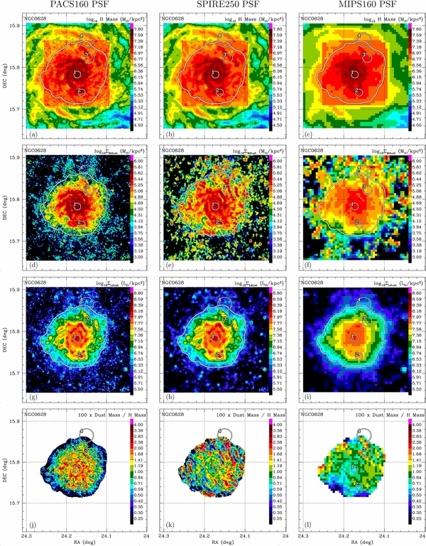
Figure 4. NGC 628 at the resolution of PACS160 (left), SPIRE250 (center), and MIPS160 (right). PACS160 resolution models are based only on IRAC, MIPS24, and PACS data; SPIRE250 resolution models are based on IRAC, MIPS24, PACS, and SPIRE250 data; MIPS160 resolution models are based on all (IRAC, MIPS, PACS, SPIRE) data. Row 1: surface density of H (both H i and H2) for XCO, 20 = 4 (see the text). Row 2: estimated dust surface density  (see the text). Row 3: dust luminosity surface density
  . Row 4: dust/H mass ratio over the main galaxy. The irregular white contour is the boundary of the "galaxy mask" (see the text). White circles are selected apertures (see Figure 8).
Download figure:
Standard image High-resolution imageWe note that the dust/H mass ratio maps change significantly when the modeling is done at the different resolution/camera combination (see the last row of Figure 4). These discrepancies are mainly due to the low sensitivity of the PACS cameras in the low-surface brightness areas (compare the MIPS and PACS flux in the outer parts of the galaxies in Figures 1 and 2), and discrepancies in the high surface brightness areas. In Section 7 we discuss the PACS–MIPS photometry discrepancies further.
6.1.2. Maps of qPAH and Starlight Parameters
Figure 5 shows maps of the PAH abundance qPAH (panels (a)–(c)), the starlight intensity parameter Umin (panels (d)–(f)), and the PDR fraction fPDR (panels (g)–(i)), over the "galaxy mask" region where the galaxy is well detected. The GM for NGC 628 has a diameter of ∼0 16, or 20 kpc at 7.2 Mpc.
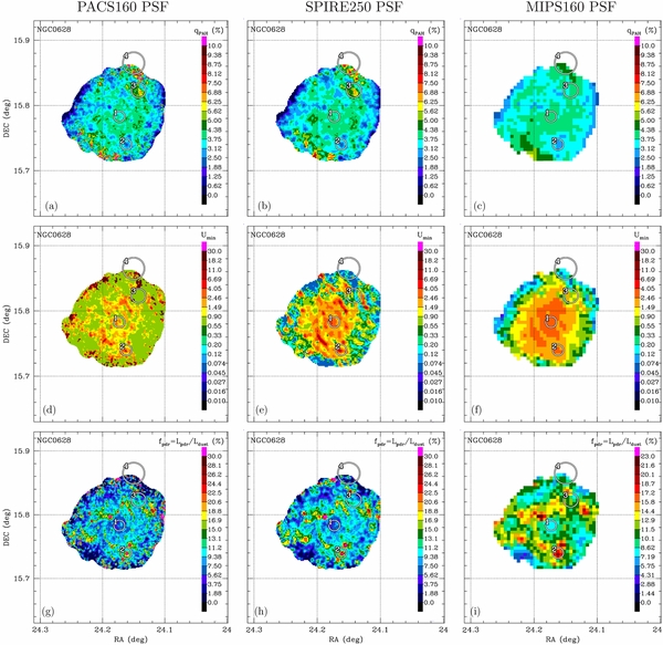
Figure 5. NGC 628 dust models at the resolution of PACS160 (left), SPIRE250 (center), and MIPS160 (right). Top row: PAH abundance parameter qPAH. Middle row: diffuse starlight intensity parameter Umin. Bottom row: PDR fraction fPDR.
Download figure:
Standard image High-resolution imageThe PAH abundance parameter qPAH, shown in Figures 5(a)–(c), is remarkably uniform over the region where it can be reliably estimated. In Figure 5(c), qPAH varies from a high of ∼0.05 a few kpc from the center down to ∼0.035 near the edge of the galaxy mask. If there is a radial gradient in qPAH, it is weak, consistent with the weak gradients found for the SINGS sample (including NGC 628) by Muñoz-Mateos et al. (2009).
At PACS160 resolution, the starlight intensity parameter Umin (see Figure 5(d)) varies between ∼0.6 and ∼3 over most of NGC 628, following the galaxy structures, but near the edges of the galaxy mask Umin appears to rise. This is because the reduced S/N results in PACS70/PACS160 ratios that appear to be anomalously high, leading to high inferred values of Umin for some pixels. This is probably the result of low PACS160 fluxes for those pixels, making it appear that the dust is rather warm. We see that when SPIRE250 data are introduced (Figure 5(e)), we have many fewer high values of Umin near the edge of the galaxy mask, and the Umin values in the brighter regions appear well behaved. This continues when the MIPS160, SPIRE350, and SPIRE500 data are brought into the fit in the MIPS160 resolution image (Figure 5(f)).
The bottom row of Figure 5 (panels (g)–(i)) shows fPDR, the fraction of the dust luminosity coming from dust heated by starlight intensities U > 100, which we expect to be associated with star-forming regions. At PACS160 resolution, most of the galaxy has fPDR ≈ 0.03 and some small bright regions (for example, the center of aperture 2 in Figure 8) have higher values, up to fPDR ≈ 0.3. These regions with high values of fPDR generally coincide with Hα peaks, and also with the regions of the highest dust luminosity per area (see Figure 4(g)). As we shift to coarser modeling (i.e., using PSFs with larger FWHM), the fPDR peaks are smoothed, and the general galaxy pixels tend to have larger fPDR values: the dynamic range of values of fPDR decreases. At MIPS160 resolution, most of the galaxy has fPDR > 0.05. The overall (dust-luminosity-weighted) mean for the galaxy is 〈fPDR〉 = 0.116: 11.6% of the total IR power is radiated by dust in regions where U > 100.
Unfortunately, at MIPS160 resolution the arm structure of both galaxies is not clearly resolved (see the MIPS160 images of the galaxies in panel (f) of Figures 1 and 2). Therefore, we cannot reliably study variation of the dust parameters between arm and interarm regions. A subsequent work (L. K. Hunt et al. 2012, in preparation) will study radial variations in the model parameters.
6.1.3. Comparison between Observed and Modeled Flux Densities
How well does the dust model reproduce the SPIRE photometry? Figure 6 shows the ratios of model-predicted intensity to observed intensity at λ = 250, 350 and 500 μm for dust models obtained by fitting photometry with PACS160, SPIRE250, and MIPS160 resolution. In order to make the comparison, we degrade either the observed image or the model-predicted image to a common resolution (i.e., when the modeling is done at PACS160 resolution, we convolve the model-predicted SPIRE250 image to the SPIRE250 PSF, and when the modeling is done at MIPS160 resolution, we convolve the observed SPIRE250 image to the MIPS160 PSF). Except near the edge of the galaxy mask (where the low S/N in the PACS data becomes an issue), the modeling tends to overpredict the SPIRE500 photometry—there is no evidence for a significant mass of very cold dust radiating only at the longer wavelengths.
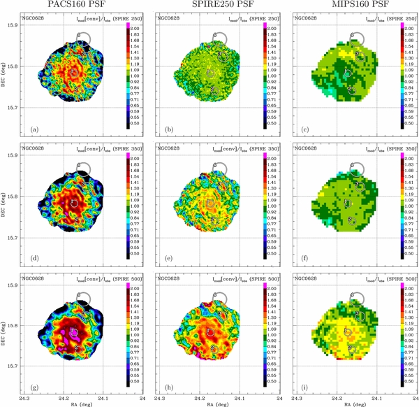
Figure 6. Ratio of model/observed intensity at λ = 250 μm (top row), λ = 350 μm (middle row), and λ = 500 μm (bottom row) for NGC 628. Left column: PACS160 PSF, model constrained only by IRAC, MIPS24, and PACS. Center column: SPIRE250 PSF, model constrained by IRAC, MIPS24, PACS, and SPIRE250. Right column: MIPS160 PSF, model constrained by all 13 cameras. The model in the center column does a fairly good job in predicting the emission at λ = 350 μm, and λ = 500 μm, except near the edge where the S/N is low. The model in the right column is in excellent agreement with all three SPIRE bands. In all panels the model predicted and observed intensities have been convolved to a common PSF before taking the ratios.
Download figure:
Standard image High-resolution imageWhen we attempt to model at PACS160 resolution (using only IRAC, MIPS24, and PACS data to constrain the model), the model predictions at SPIRE250, SPIRE350, and SPIRE500 do not agree very well with observations (see Figures 6(a), (d), and (g)). If we coarsen the modeling to SPIRE250 resolution and add SPIRE250 to the model constraints, we now reproduce the SPIRE250 image (not surprising) and the model predictions at 350 μm and 500 μm are within ±30% and ±50% of the SPIRE observations, respectively, over most of the galaxy mask. If we further coarsen the modeling to the MIPS160 PSF, and use all the data to constrain the model, we find good agreement at all SPIRE bands (see Figures 6(c), (f), and (i)), with only SPIRE500 slightly overpredicted by ≈10% in some regions.
Figures 6(c), (f), and (i) show that when all of the cameras are used to constrain the modeling (and with the improved S/N of the larger MIPS160 pixels), the model emission is generally in good agreement with the SPIRE imaging—for all three SPIRE bands the ratio of model/observation is close to 1 over most of the galaxy, with significant departures only just at the edge of the galaxy mask, where observational errors are likely to be the explanation.
6.1.4. Global SED Fitting
Figure 7 shows global SEDs for NGC 628. The observed photometry is represented by rectangular boxes (Spitzer (IRAC, MIPS) in red; Herschel (PACS(S), SPIRE) in blue). The model convolved with camera response function (i.e., expected camera photometry for the model) is represented by diamonds (Spitzer in red, Herschel in blue). The two rows show the global SED for NGC 628. The observed global photometry for NGC 628 is the same across the two top rows, but the models differ. Each black curve is a fitted model spectrum. The diamonds show the fitted model spectrum convolved with the instrumental response function for each camera, i.e., the expected photometry for the fitted model.

Figure 7. Model SEDs for NGC 628. Black line: total model spectra. Cyan line: stellar contribution. Dark red line: emission from dust heated by the power-law U distribution. Dark green line: emission from dust heated by U = Umin. Solid-line rectangles: observations used in the fit (red: Spitzer (IRAC, MIPS); blue: Herschel (PACS(S), SPIRE)). Dashed-line rectangles: observations not used in the fit (same color scheme as solid-line rectangles). Diamonds: model convolved with camera response function (i.e., expected camera photometry of the model) (red: Spitzer; blue: Herschel). Top row: global SED compared with single-pixel models. Second row: global SED, for multi-pixel model. In the left column, only IRAC, MIPS24, and PACS are used in the fit (MIPS70,160 and SPIRE are not used), yet the model nevertheless falls close to the observed SPIRE fluxes. In the center column, IRAC, MIPS24, PACS, and SPIRE250 are used (i.e., MIPS70,160 and SPIRE350,500 are not used), and the agreement with SPIRE is improved. In the right column, all IRAC, MIPS, PACS, and SPIRE data are used to constrain the model, and the agreement with all SPIRE bands is excellent, although the model slightly overpredicts the emission at 350 μm and 500 μm.
Download figure:
Standard image High-resolution imageThe top row shows "single-pixel" models for the galaxy based on (a) IRAC, MIPS24, and PACS data only, (b) IRAC, MIPS24, PACS, and SPIRE250, and (c) IRAC, MIPS, PACS, and SPIRE (all the cameras).
The second row shows the predicted model SED obtained by fitting a dust model to each resolved pixel, and then summing the emission over all the pixels. These predicted SEDs differ from the previous "single pixel" predicted SED because the dust modeling is a nonlinear process. The total dust mass predicted in this way is, however, similar to the "single-pixel" prediction (see Section 8 for details). When the modeling is done at lower resolutions (MIPS160) the "single pixel" and map-averaged quantities are in closer agreement.
6.1.5. Fitting in Selected Apertures
Figure 8 shows SEDs for four circular apertures located on NGC 628, sampling a wide range of surface brightnesses,  (see Figure 4 for aperture locations). Aperture 4 is located partially outside the galaxy mask, where the single-pixel dust modeling is not reliable, but the improved S/N of a large aperture allows reliable determination of the dust model parameters. We fit the DL07 model to the summed flux within each aperture. The top row shows the SED for a 60'' (diameter) circular aperture centered on the galaxy nucleus. The second row shows the SED for a 60'' aperture located on a bright spot on the spiral arms. We observe that the PACS photometry is larger than the corresponding MIPS photometry in the high surface brightness apertures 1 and 2. When both data sets are included in the modeling, the dust model gives values intermediate between PACS and MIPS. The third and fourth rows show SEDs in 80'' and 120'' apertures further from the center. We employ larger apertures in order to obtain reasonable S/N in these fainter regions. In aperture 4, the MIPS and PACS photometry differ significantly. When SPIRE, MIPS70, and MIPS160 are not used (e.g., in the PACS160 resolution modeling, Figure 8(j)) the high PACS70/PACS160 ratio causes the model to infer very high values of Umin and low values of
  , and hence to underpredict the SPIRE photometry. When we include SPIRE250 (Figure 8(k)) the model can reproduce SPIRE250, but continues to underpredict SPIRE350 and SPIRE500. Finally, when SPIRE350,500 and MIPS70,160 are added as constraints (Figure 8(l)), the modeling improves dramatically in aperture 4 and other low-brightness areas, reproducing most of the data, and making it clear that PACS70 is an outlier.

Figure 8. Model SEDs for four selected apertures on NGC 628. See Figure 4 for aperture location, and Figure 7 for an explanation of the color coding. Top row: 60'' (circular) aperture centered on the galaxy nucleus. Second row: 60'' aperture located on a bright spot on the spiral arms. Third row: 80'' aperture in a mid-luminosity region. Bottom row: 120'' aperture in a low-luminosity region.
Download figure:
Standard image High-resolution imageThe astute reader will note that the estimated uncertainties for, e.g., the PACS100 global photometry differ between the columns (i.e., for fluxes extracted after convolving to different PSFs). For each PSF, we estimate the noise per pixel based on the pixel statistics in the background region (see Appendix D). We then make a simple assumption concerning the pixel-to-pixel noise correlation. The fact that the uncertainty estimates for the aperture fluxes depend on the PSF is an indication that our assumption about the correlated component of the noise is imperfect. This is only an issue for the faint, low S/N data, such as the PACS fluxes in apertures 3 and 4.
In aperture 4 (Figure 8, last row), the model uses γ = 1, i.e., the dust is heated almost entirely by a power-law U distribution, but with very high values of γ. This corresponds to a broad distribution of starlight intensities in the U ≳ Umin range, with very little power in the high intensity range (PDR). This may be an artifact arising from the large photometric uncertainties.
6.2. NGC 6946
NGC 6946, an active star-forming galaxy, is classified as SABcd. At a distance D = 6.8 Mpc, the total H i mass is  (Walter et al. 2008), with 42% of the H i falling within the galaxy mask. The H2 mass within the galaxy mask is M(H2) = (8.6 ± 0.6) × 109(XCO, 20/4) M☉ (Leroy et al. 2009). As discussed previously, we adopt XCO, 20 = 4 as a global estimate. The star formation rate is estimated to be 4.5 M☉ yr−1 (Calzetti et al. 2010). NGC 6946 is remarkable for hosting at least nine supernovae over the past century (Prieto et al. 2008).
The variable carbon star V0778 Cyg, located near R.A. = 309.044, decl. = 60.082 (slightly off the bottom left corner of the maps shown in Figures 9–11), saturates the IRAC and MIPS detectors. The associated image artifacts affect the background estimation and subtraction, making the modeling less reliable in the bottom left corner of the maps.
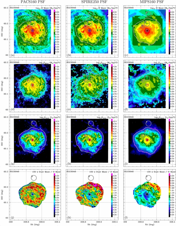
Figure 9. NGC 6946 at the resolution of PACS160 (left), SPIRE250 (center), and MIPS160 (right). Row 1: surface density of H i and H2 for XCO, 20 = 3 (see the text). Row 2: dust surface density  . Row 3: dust luminosity surface density
  . Row 4: dust/H ratio over the main galaxy. The irregular white contour is the boundary of the "galaxy mask," within which the S/N is high enough to obtain reliable estimates of dust and starlight parameters. White circles are selected apertures (see Figure 13).
Download figure:
Standard image High-resolution image
Figure 10. NGC 6946 dust models at the resolution of PACS160 (left), SPIRE250 (center column), and MIPS160 (right). Top row: PAH abundance parameter qPAH. Middle row: diffuse starlight intensity parameter Umin. Bottom row: PDR fraction fPDR.
Download figure:
Standard image High-resolution image
Figure 11. Similar to Figure 6, but for NGC 6946. Ratio of model intensity/observed intensity for NGC 6946 at λ = 250 μm(top row), λ = 350 μm (middle row), and λ = 500 μm(bottom row). Left column: PACS160 PSF, model constrained only by IRAC, MIPS24, and PACS. Center column: SPIRE250 PSF, model constrained by IRAC, MIPS24, PACS, and SPIRE250. Right column: MIPS160 PSF, model constrained by all 13 cameras. The model in the center column does a fairly good job in predicting the emission at λ = 350 μm, and λ = 500 μm, except near the edge where the S/N is low. The model in the right column is in excellent agreement with all three SPIRE bands.
Download figure:
Standard image High-resolution image6.2.1. Dust and H Mass Maps
Figure 9 shows maps of the gas in NGC 6946 obtained from the THINGS 21 cm map (Walter et al. 2008) and the HERACLES CO 2–1 map (Leroy et al. 2009), convolved to the resolution of PACS160, SPIRE250, and MIPS160. The second row shows dust maps obtained by the present study. The dust map obtained using the PACS160 PSF has dust clearly visible only out to a radius of ∼250'' (8 kpc at 6.8 Mpc), but the 11'' (500 pc) FWHM of the beam resolves the spiral structure. The arm/interarm contrast in dust surface density appears to be approximately a factor of ∼2 in this image. Introducing SPIRE 250 μm data requires the PSF to be broadened, making the spiral arms less apparent, but allows dust to be detected out to larger radii, notably in the northern spiral arm. The MIPS160 resolution image clearly shows dust in the northern spiral arm out to a distance of ∼15 kpc from the nucleus.
The dust luminosity/area  (Figure 9, bottom row) peaks at ∼1010.1 L☉ kpc−2 in the nucleus (see the PACS160 resolution map), and can be followed down to
  in the MIPS160 resolution map. Similarly, the IR luminosity/area contributed by PDRs peaks at
  near the center, and is reliably measured down to ∼105.6 L☉ kpc−2.
The dust/H mass ratio shown in Figures 9(j)–(l), calculated assuming XCO, 20 = 4, shows a pronounced minimum of ∼0.005 in the central kpc. In this region the gas is primarily molecular, and the estimated dust/H mass ratio is therefore sensitive to the value assumed for XCO. NGC 6946 has approximately solar metallicity, and we expect the dust/H mass ratio to be ∼0.01. The surprisingly low dust/H mass ratios found in the center of NGC 6946 indicate that the value of XCO near the center should be about a factor of ∼2 smaller than the value XCO, 20 = 4 adopted for the bulk of the galaxy. This conclusion is consistent with interferometric studies of giant molecular clouds (GMCs) which indicate XCO, 20 ≈ 1.25 near the center of NGC 6946 (Donovan Meyer et al. 2012), using virial mass estimates for individual GMCs.
6.2.2. Maps of qPAH and Starlight Parameters
The PAH abundance qPAH in NGC 6946 rises from a minimum of ≲ 1% near the nucleus, reaching levels of ∼(4 ± 1)% at distances ∼1–8 kpc from the center, ultimately appearing to decline at the edge of the detectable region. The central minimum in qPAH is real (it is independent of uncertainties in the appropriate value of XCO). The local minimum of qPAH at the center may be the result of destruction of PAHs by processes associated with star formation (there is no evidence of active galactic nucleus activity in NGC 6946). We note that there are a number of other local minima of qPAH evident in Figures 10(a)–(c); just as for the central minimum, these extranuclear minima tend to coincide with peaks in dust luminosity surface brightness  (see Figures 9(g) and (h)) and peaks in fPDR (see Figures 10(j), (k), and (l)). These are both indicators of luminous star-forming regions, which can be expected to coincide with H ii regions around hot stars, which appear to destroy PAHs (e.g., Povich et al. 2007). Supernova blast waves are presumed to also destroy PAHs.
Because the outer falloff in qPAH is occurring as the S/N is falling to low values, it is not certain whether the observed decline is real or an artifact of different levels of background subtraction at different wavelengths. However, the decline in qPAH in the outer regions persists in the MIPS160 resolution map. These variations in qPAH will be examined in more detail in future studies.
The diffuse starlight intensity parameter Umin (Figure 10, middle row) shows a general decline with increasing distance from the center. The PACS160 resolution map of Umin is somewhat noisy, particularly in the outer regions, but the MIPS160 resolution map of Umin shows a systematic decline from values as high as Umin ≈ 10 in the central ∼500 pc down to Umin ≈ 0.15 in the outer regions, ∼10 kpc from the center. Even lower values of Umin are estimated for some pixels, but this is seen only at the lowest S/N levels.
The bottom row of Figure 10 shows fPDR. The behavior of fPDR in NGC 6946 is similar to NGC 628. Bright complexes coincide with local maxima of fPDR. Outside very bright complexes fPDR is quite smooth across the galaxy.
6.2.3. Comparison between Observed and Modeled Flux Densities
The model-predicted/observed flux ratios for NGC 6946 (shown in Figure 11) behave similarly to those of NGC 628 (see Figure 6). When long-wavelength data are not used in the dust model fit, the modeling tends to overpredict the intensity at the longer wavelengths. However, when the SPIRE photometry is included in the model constraints, the overprediction is greatly reduced. In the case of MIPS160 PSF (all bands used), the SPIRE250 photometry is reproduced by the model within 10%, and SPIRE500 tends to be overpredicted by less than 15%.
6.2.4. Global SED Fitting
Figure 12 shows the global SED for the galaxy NGC 6946 (similar to Figure 7 for NGC 628). The top row shows the SED for a "single-pixel" model and the second row shows the predicted model SED obtained by summing over the model SED for individual pixels. Again, we observe small differences between the global modeling (top row) and resolved studies (bottom row) due to the nonlinear behavior of the modeling process. It is seen that when the modeling is done using the MIPS160 PSF, the dust mass estimated from the multi-pixel model is in good agreement with that obtained for a single-pixel model.
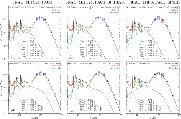
Figure 12. Model SEDs for NGC 6946. The color coding and columns are similar to Figure 7. Top row: global SED compared with single-pixel models. Second row: global SED, compared to multi-pixel model. Even when SPIRE data are employed, the model tends to overpredict (slightly) the global photometry at 500 μm.
Download figure:
Standard image High-resolution image6.2.5. Fitting in Selected Apertures
Figure 13 shows SEDs for four circular apertures located on NGC 6946, sampling a wide range of surface brightnesses,  , similar to Figure 8 for NGC 628. The top row shows the SED for a 60'' diameter circular aperture centered on the galaxy nucleus. The second row shows the SED for a 60'' aperture located on a bright spot on the spiral arms. The third and fourth rows show SEDs in 120'' apertures further from the center. Aperture 4 is located completely outside the galaxy mask, but the S/N of a large aperture allows a reliable determination of the dust model parameters.
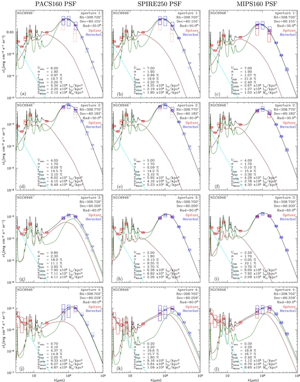
Figure 13. Model SEDs for four selected apertures on NGC 6946. See Figure 9 for aperture location, and Figure 7 for an explanation of the color coding. Top row: 60'' (circular) aperture centered on the galaxy nucleus. Second row: 60'' aperture located on a bright spot in a spiral arms. Third row: 120'' aperture in a mid-luminosity region. Bottom row: 120'' aperture in a low-luminosity region.
Download figure:
Standard image High-resolution imageThe nuclear emission is strongly peaked. The Herschel photometry for the central aperture noticeably decreases when the image is convolved to MIPS160 resolution, and the estimated dust luminosity surface brightness in the 60'' extraction aperture drops from 2.2 × 10⁹ L☉ kpc−2 (Figures 13(a) and (b)) to 1.3 × 10⁹ L☉ kpc−2 (Figure 13(c)).
We observe that the PACS photometry in the high surface brightness nucleus tends to generally be larger than the corresponding MIPS photometry—compare the PACS and MIPS fluxes in Figure 13(c). In apertures 2, 3, and 4, the PACS and MIPS photometry (at common resolution—see Figures 13(f), (i), and (l)), the PACS and MIPS photometry is in fairly good agreement. The disagreement in the PACS versus MIPS photometry is larger for NGC 6946 than for NGC 628 (see Table 6 below), presumably related to the much higher peak surface brightnesses present in NGC 6946. At MIPS160 resolution,  in NGC 628 aperture 1 is only 7% of
  in NGC 6946 aperture 1. Table 3 summarizes the main properties of the galaxies, and the results, of the modelling.
Table 3. Galaxy Properties
| NGC 628 | NGC 6946 | |
|---|---|---|
| Typea | SAc | SABcd |
| Da (Mpc) | 7.2 | 6.8 |
| Resolution at D | 1'' = 34.9 pc | 1'' = 33.0 pc |
| Galaxy optical sizeb (kpc) | 11.0 × 9.9 | 11.4 × 9.7 |
| Galaxy mask area A (kpc2) | 274 | 307 |
Galaxy mask radius  (kpc) (kpc) |
9.4 | 9.9 |
 c (M☉), total in map c (M☉), total in map |
(3.7 ± 0.2) × 109 | (5.5 ± 0.3) × 109 |
| M(H2)d (M☉), total in map | (2.5 ± 0.6) × 109 | (9.7 ± 2.7) × 109 |
 (M☉), within mask (M☉), within mask |
(1.5 ± 0.1) × 109 | (2.1 ± 0.1) × 109 |
| M(H2)d (M☉), within mask | (2.0 ± 0.2) × 109 | (8.6 ± 0.5) × 109 |
| MH (M☉), within mask | (3.5 ± 0.3) × 109 | (10.7 ± 0.6) × 109 |
| log10(O/H) + 12e | 8.27 ± 0.12 | 8.37 ± 0.06 |
| L(Hα)f (L☉), total | 1.88 × 10⁷ | 1.00 × 10⁸ |
| SFRg (M☉ yr−1), total | 0.7 ± 0.2 | 4.5 ± 1.2 |
| Fν(IRAC3.6) (Jy), within mask | 0.83 ± 0.10 | 3.13 ± 0.52 |
| Fν(IRAC4.5) (Jy), within mask | 0.57 ± 0.06 | 2.22 ± 0.32 |
| Fν(IRAC5.8) (Jy), within mask | 0.98 ± 0.23 | 4.9 ± 1.2 |
| Fν(IRAC8.0) (Jy), within mask | 2.61 ± 0.44 | 13.2 ± 2.4 |
| Fν(MIPS24) (Jy), within mask | 3.04 ± 0.33 | 18.9 ± 2.0 |
| Fν(MIPS70) (Jy), within mask | 31.5 ± 9.8 | 196 ± 55 |
| Fν(MIPS160) (Jy), within mask | 104 ± 20 | 420 ± 127 |
| Fν(PACSS70) (Jy), within mask | 39 ± 12 | 245 ± 58 |
| Fν(PACSS100) (Jy), within mask | 73 ± 21 | 433 ± 122 |
| Fν(PACSS160) (Jy), within mask | 110 ± 20 | 526 ± 126 |
| Fν(SPIRE250) (Jy), within mask | 59.5 ± 7.0 | 247 ± 29 |
| Fν(SPIRE350) (Jy), within mask | 27.4 ± 3.3 | 101 ± 12 |
| Fν(SPIRE500) (Jy), within mask | 10.5 ± 1.4 | 35.4 ± 4.2 |
| Md (M☉), within mask | (2.9 ± 0.4) × 107 | (6.7 ± 0.6) × 107 |
| 100 × Md/MH, within mask | 0.82 ± 0.17 | 0.63 ± 0.09 |
| Ld (L☉), within mask | (6.8 ± 0.4) × 109 | (3.3 ± 0.3) × 1010 |
| LPDR (L☉), within mask | (7.9 ± 1.4) × 108 | (4.7 ± 0.8) × 109 |
| 〈Umin〉, within mask | 1.6 ± 0.3 | 3.1 ± 0.6 |
 , within mask , within mask |
1.7 ± 0.3 | 3.6 ± 0.6 |
| 〈fPDR〉, within mask | (11.6 ± 1.3)% | (14.2 ± 2.8)% |
| 〈qPAH〉, within mask | (3.7 ± 0.3)% | (3.6 ± 0.4)% |
Notes. aFrom Kennicutt et al. (2011). bMajor and minor radii at μB = 25 mag arcsec−2 isophote, from Kennicutt et al. (2011). cWe use the "Natural" (NA) weighting maps (see Walter et al. 2008 for details). dFrom Leroy et al. (2009), for XCO, 20 = 4 (see the text). ePT05 H ii region abundances, unweighted average, from Moustakas et al. (2010). fFrom Kennicutt et al. (2008), uncorrected for internal extinction. gStar formation rate; from Calzetti et al. (2010), based on Hα+24 μm.
Download table as: ASCIITypeset image
7. IMPORTANCE OF SPIRE PHOTOMETRY
We investigate the effect of only using certain sets of cameras in our resolved (multi-pixel) modeling, since this situation will arise in galaxies that were only observed with some of the instruments. Dust estimates for NGC 628 and NGC 6946 based on different camera combinations are shown in Figure 14, where we compare the dust mass estimate with our "gold standard," the dust mass estimate using all cameras, at MIPS160 resolution.33
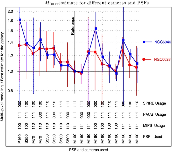
Figure 14. Total dust mass Md (summed over all pixels) estimated for NGC 628 and NGC 6946 using different camera/PSF combinations (see the text). Masses are given relative to the "best estimate" Md obtained summed over all pixels using all wavelengths and MIPS160 resolution.
Download figure:
Standard image High-resolution imageIn Figures 14–17 the horizontal axis represents different combinations of PSF and cameras. The nomenclature convention is as follows. The first characters describe the PSF used; P160, S250, S350, S500, M70, and M160 refer to PACS160, SPIRE250, SPIRE350, SPIRE500, MIPS70, and MIPS160, respectively.
The first group of three digits refers to the MIPS24, MIPS70, and MIPS160 cameras, with one indicating usage. The next set of three digits similarly indicates usage of the three PACS bands, and the final three digits correspond to usage of the SPIRE cameras. For example, S350 110 111 110 uses MIPS24, MIPS70, PACS70, PACS100, PACS160, SPIRE250, and SPIRE350 cameras at SPIRE350 PSF. We always use the Scanamorphos data reduction for PACS.
The 10 right-most columns correspond to the MIPS160 PSF, and the remaining eight left-most columns have different PSFs (sorted by ascending FWHM left to right). The modeling done at MIPS160 resolution uses different camera combinations, allowing one to examine, at fixed angular resolution, the effects of different wavelength coverage and PACS/MIPS discrepancies.
Figure 14 shows that the dust mass estimates for these two galaxies appear to be quite good when we use the three SPIRE bands: the total dust mass estimated without using MIPS160 (at MIPS160 or SPIRE500 PSF) is off by only ∼10%. It therefore appears that resolved maps of dust in nearby galaxies can be reliably obtained at the resolution of SPIRE500. The dust mass estimates appear to be good provided at least two SPIRE bands (SPIRE250 and SPIRE350) are employed: the total dust mass estimated without using SPIRE500 and MIPS160 is off by 30% for NGC 628, and 22% for NGC 6946. The S250 100 111 100 dust map yields a global dust mass that exceeds the best estimate by ∼38%. For some purposes this ∼38% loss of accuracy will be acceptable, as it makes possible a dust map with FWHM = 182.
In order to map the dust at higher angular resolution (PACS160 PSF), we can only use a subset of all the cameras available (IRAC, MIPS24, PACS). Dust maps made at the resolution of PACS160 are less reliable, for three reasons: (1) with smaller pixels, the S/N of the image is poor in the faint regions, (2) there seem to be significant systematic uncertainties associated with the PACS photometry, (3) the dust models are unconstrained at λ > 160 μm, and (4) our PACS maps are less sensitive than the MIPS counterparts. The nonlinearity of the dust model fitting procedure can result in large errors in dust mass in the low S/N regions. Dust masses estimated using maps at PACS160 resolution (using IRAC, MIPS24, and PACS data only) can overestimate the dust masses by factors ≈1.4–1.8. If greater accuracy is required, PACS160 resolution should only be used in the highest surface brightness regions, where S/N issues should be less critical.
It has sometimes been argued that dust masses estimated using only data at wavelengths λ ⩽ 160 μm (e.g., those based on MIPS photometry only) are suspect because the observations are insensitive to "cold" dust at temperatures Td ≲ 12 K. The SINGS sample included 17 galaxies with SCUBA 850 μm, and Draine et al. (2007) found that reliable dust mass estimates could be obtained with the DL07 dust model without using data longward of 160 μm: these galaxies did not appear to contain significant masses of "cold dust." The SPIRE photometry for NGC 628 and NGC 6946 confirms this: these galaxies do not appear to contain substantial masses of cold dust. In fact, we find that models fitted to the PACS photometry alone tend to predict more emission at long wavelengths than is observed. This is evident in Figures 6(a) and (d), and Figures 11(a) and (d), which show that DL07 dust models based only on λ ⩽ 160 μm data (IRAC, MIPS24, and PACS) tend to overpredict the actual fluxes at 250 and 500 μm in the central 6 arcmin (12 kpc). This is also seen in Figures 7(d) and 12(d), which compare the observed global SED with the sum of the SEDs from a multi-pixel model for each galaxy. The model (the diamonds) overpredicts the SPIRE data by factors of ∼1.1, 1.2, and 1.2 at 250, 350, and 500 μm. This is rather good agreement, and indicates that there is no substantial amount of very cold dust present in either galaxy. In fact, when the SPIRE data are used to constrain the fit, the best-fit models actually raise the starlight intensities slightly in order to match both the PACS, MIPS, and SPIRE photometry, reducing the dust mass estimate. Note the very good agreement between observed and model SEDs in Figures 7(f) and 12(f), where all data are used to constrain the multi-pixel fit.
The main difference in the estimated dust masses in the different PSF/cameras combination is due to the different values of Umin found when we do not use all the cameras available. Figure 15 shows 〈Umin〉 (defined in Equation (23)), the dust-mass-weighted value of the starlight intensity parameter Umin relative to the best estimate for 〈Umin〉—the estimate obtained using all the data at MIPS160 resolution.

Figure 15. 〈Umin〉 (weighted mean over the pixels) estimated using different cameras and PSFs relative to the best estimate (obtained with all cameras and MIPS160 PSF).
Download figure:
Standard image High-resolution image8. MAPS VERSUS GLOBAL PHOTOMETRY
The KINGFISH sample consists of galaxies that are near enough to be well resolved, enabling us to make maps of dust and starlight properties. However, because the dust modeling used here is a nonlinear procedure, the total dust mass estimate, for example, will depend on what resolution is employed. In the preceding sections, we usually made dust maps using the best angular resolution possible with each chosen camera set used, with the limiting resolution therefore determined by the longest wavelength data used in the fit (or the inclusion of MIPS160).
Herschel is frequently used to observe distant galaxies that are unresolved at the longest wavelengths. For the KINGFISH galaxies, we will therefore also estimate dust masses using the global photometry (the flux from within the galaxy mask), to see how dust mass estimates based on global photometry compare with the best estimates for a well-resolved galaxy.
Figure 16 shows the dust mass estimated using the DL07 dust models to fit the global SED, divided by the "gold standard," i.e., the sum of the dust mass obtained from pixel-by-pixel modeling of the resolved galaxy in the MIPS160 PSF using all the cameras. Recall that the DL07 model assumes that most of the dust is exposed to a single starlight intensity Umin. A multi-pixel model with Umin, j varying from pixel to pixel cannot be exactly reproduced by a model that assumes a single value of Umin for the entire galaxy, hence fitting the summed photometry with a single-pixel model will in general give a dust mass that will differ from that obtained by summing over a multi-pixel model.
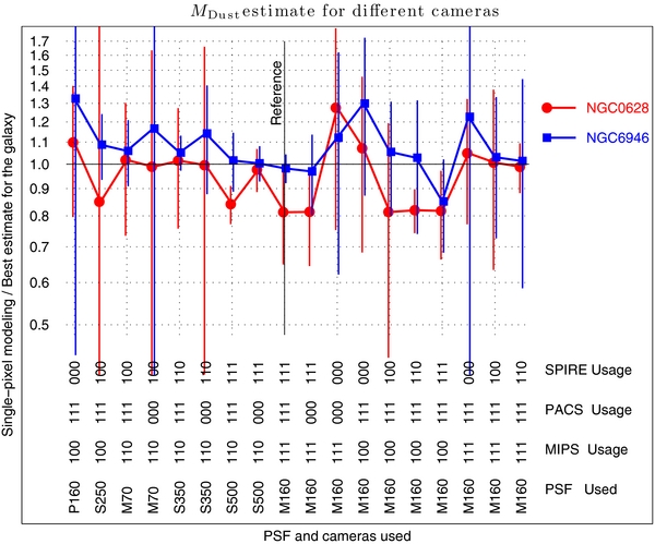
Figure 16. Dust mass estimates based on global photometry for NGC 628 and NGC 6946, using different camera combinations, relative to the sum of the dust mass (obtained from pixel-by-pixel modeling of the resolved galaxy) in the MIPS160 PSF using all the cameras (i.e., relative to the best total dust estimate for the galaxies). In principle, estimates based on global photometry should not depend on the chosen PSF, only on the camera combination. In practice, flux scattered out of the galaxy mask (into the PSF's extended wings) changes the global photometry estimates, leading to small differences in the parameter estimates (e.g., see differences between P160 100 111 000 and M160 100 111 000 modeling).
Download figure:
Standard image High-resolution imageFigure 16 shows that if all (IRAC, MIPS, PACS, SPIRE) data are used, the dust mass obtained by fitting the global SED is very close to that obtained from a multi-pixel fit of the resolved galaxy: the global dust mass is within 18% of the best estimate for NGC 628, and within 3% of the best estimate for NGC 6946. If data from some cameras are not used, the single-pixel estimate for the dust mass will of course change, but we see that for NGC 628 and NGC 6946 the resulting dust masses vary surprisingly little provided we have SPIRE data or MIPS160. If we use only PACS for λ ⩾ 70 μm, the dust mass estimate for NGC 628 is high by ∼10%. The M160 111
111 000
000 000 column in Figure 16 compares the global dust mass estimated from a single-pixel fit using only Spitzer (IRAC and MIPS) data versus our "gold standard" best estimate (multi-pixel model using all cameras). The dust masses estimated using only the global photometry from Spitzer are within ∼30% of our present best estimates. Thus, at least for normal-metallicity star-forming galaxies such as NGC 628 and NGC 6946, dust mass estimates based on IRAC and MIPS photometry, e.g., the dust masses estimated for the SINGS sample (Draine et al. 2007) appear to be reliable.
Figure 17 compares the global dust mass estimated using global fluxes to the dust masses estimated summing the dust masses over each map, for different sets of cameras. Essentially, it is a measure of the nonlinear behavior of the dust modeling. For each camera and PSF combination, performing resolved modeling allows the dust to be colder in some regions, and this introduces more dust mass. Modeling based on global photometry underpredicts the dust masses by 0%–20% in most cases.
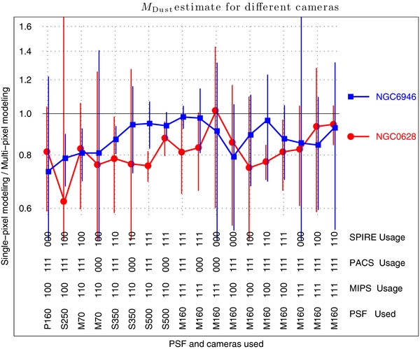
Figure 17. Dust mass estimates based on global photometry for NGC 628 and NGC 6946, using different camera combinations, relative to the sum of the dust mass obtained from pixel-by-pixel modeling of the resolved galaxy using the same camera set.
Download figure:
Standard image High-resolution imageIn principle, using the MIPS160 PSF results as our "gold standard" best estimate for the dust parameters may also suffer from the above-mentioned nonlinear behavior: each MIPS160 pixel covers a rather large area of the galaxy, in which the dust properties (e.g., qPAH) or radiation field (e.g., Umin) may have variations. Unfortunately, the discrepancy of PACS160 and MIPS160 fluxes makes it important to retain MIPS160 photometry, and, therefore, to use the broader MIPS160 PSF.
Table 4 summarizes the main parameters obtained by single-pixel and multi-pixel modeling of the galaxies at MIPS160 resolution, using all the cameras.
Table 4. Multi-pixel and Single-pixel Best-fit Model Parameters at MIPS160 Resolution
| NGC 628 | NGC 6946 | |||
|---|---|---|---|---|
| Parameter | Resolveda | Globalb | Resolveda | Globalb |
| Md (M☉) | 2.87 × 10⁷ | 2.33 × 10⁷ | 6.74 × 10⁷ | 6.62 × 10⁷ |
| Ld (L☉) | 6.83 × 10⁹ | 7.08 × 10⁹ | 3.31 × 10¹⁰ | 3.20 × 10¹⁰ |
| Umin | 1.46 | 2.00 | 3.05 | 3.00 |
 |
1.75 | 2.23 | 3.61 | 3.55 |
| 100 × fPDR | 11.6 | 10.2 | 14.2 | 15.3 |
| 100 × qPAH | 3.67 | 3.70 | 3.55 | 3.30 |
| 100 × Md/MHc | 0.82 | 0.66 | 0.63 | 0.61 |
Notes. aTotal or mean values are defined in Equations (21)–(24). bValues are from a model fit to the global photometry. cFor XCO, 20 = 4.
Download table as: ASCIITypeset image
9. ALTERNATIVE PARAMETERIZATIONS OF THE STARLIGHT INTENSITY DISTRIBUTION
Recently Galliano et al. (2011), in a resolved study of the dust in the LMC, advocated a starlight heating intensity distribution function different from what is employed in the current work. They recommended using the starlight distribution function of Dale & Helou (2002), with a power-law distribution between two adjustable parameters Umin and Umax, with adjustable power-law exponent α. We note that Galliano et al. (2011) use a slightly different nomenclature: Umax ≡ Umin + ΔU. The distribution used in the present work (Equations (9) and (10)) incorporates an additional "delta function" component at Umin, but fixes the value of Umax = 107.
Galliano et al. (2011) claimed that satisfactory fits can be obtained without the "delta function" component. We note that while we fix Umax to a given value in our model, Galliano et al. (2011) use Umax as a free parameter. Both models have thus the same number of degrees of freedom. Galliano et al. (2011) based their claim on maps of the LMC using IRAC, MIPS, and SPIRE. Here we test this claim using our maps of NGC 628 and NGC 6946.
Figure 18 shows maps of χ2 (goodness of fit) obtained for three different starlight distribution schemes, all done at MIPS160 resolution, using all 13 cameras. The top row images correspond to NGC 0628 and the bottom row images correspond to NGC 6946. In the left column the starlight distribution is a power law between Umin and Umax with power-law exponent α (all adjusted) without the delta function contribution at Umin, as proposed by Galliano et al. (2011). It has six adjustable parameters (Ω⋆, Mdust, qPAH, Umin, Umax, α), and therefore 13 − 6 = 7 degrees of freedom per pixel. The fit for this starlight distribution is poor, giving χ2 in the range 10–20 in the bright regions of the galaxies. In the middle column the starlight distribution is a power law between Umin and fixed Umax = 107, with power-law exponent α (only Umin and α are adjusted), plus a delta function contribution at Umin. This fit produces excellent results and is the one recommended in the present work. We note that this fit has the same number of degrees of freedom as the ones in the left column panels; the adjustable parameter Umax is replaced by the normalization of the "delta function" via the parameter γ. In the right column the starlight distribution is a power law between Umin and Umax with power-law exponent α (all adjusted), plus a delta function contribution at Umin. Although the right panels have one extra adjustable parameter (Umax) with respect to the recommended fit, the fit quality is similar to the middle panels. If Umax were a relevant parameter, one would expect χ2 to decrease significantly (of order 1). In fact, in the right column fit, for most of the bright pixels the best-fit Umax value is Umax = 107 and thus the value of χ2 is for those pixels exactly the same as in the center column fit.
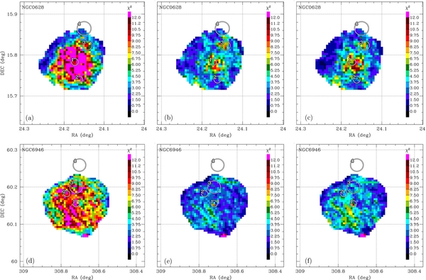
Figure 18. Comparison of χ2 (goodness of fit) of three different starlight distribution schemes. In the left column the starlight distribution is of the form proposed by Dale & Helou (2002) and recently favored by Galliano et al. (2011): a power law between Umin and Umax (both adjusted) without the delta function contribution at Umin. The fit for this starlight distribution is poor. In the center column the starlight distribution is of the form used in the present modeling: a power law between Umin and Umax = 107, plus a delta function contribution at Umin. This fit produces excellent results. In the right column the starlight distribution is a power law between Umin and Umax (both adjusted), including a delta function contribution at Umin. Although the right panels have one extra degree of freedom (Umax), the fit quality is similar to the middle panels. The top row is for NGC 628 and the bottom row is for NGC 6946. The power-law exponent α is treated as an adjustable parameter in all the fits.
Download figure:
Standard image High-resolution imageWe found that the χ2 values of the distribution used in the current work are significantly smaller than the ones found using the Galliano et al. (2011) distribution. Therefore, we recommend adding the "delta function" component at Umin. Since the fit does not improve significantly by allowing Umax to be fitted, we recommend fixing it to Umax = 107, leading to a simpler, more robust fit. It should be noted that the Galliano et al. (2011) study is based on the dust in the LMC, and in our present work we use NGC 628 and NGC 6946, two galaxies with metallicities closer to the MW metallicity. Additionally, due to the proximity of the LMC, each pixel covers a physical area much smaller than our modeling pixels.
10. DISCUSSION
10.1. Dust Mass Estimation
Dust mass estimates are, of course, model dependent. Above we have estimated the dust mass using a specific dust model, the DL07 silicate-graphite-PAH model, with an assumed parametric form for the starlight intensities heating the dust. The physical dust model and the ansatz for the distribution of starlight intensities together appear to successfully reproduce the observed SEDs, and to give reliable estimates of the dust masses.
As discussed in Section 4, the far-infrared opacity of the amorphous silicate originally put forward by DL84 was subsequently adjusted slightly (Li & Draine 2001) to improve agreement with the far-infrared and submillimeter emission observed for the local high-latitude dust. Thus the DL07 model uses dust properties that can reproduce the observed FIR-submillimeter emission from the MW cirrus with a single starlight heating intensity—no "cold dust" is needed for the MW cirrus. In this dust model, the opacities are assumed to be independent of the dust temperatures.
Here we see that the same dust model, with suitable adjustment of the starlight assumed to be heating the dust, is able to reproduce the emission from NGC 628 and NGC 6946 out to 500 μm, without introducing any "cold dust" component. The modeling performed at MIPS160 resolution, using all the IRAC, MIPS, PACS, and SPIRE cameras, in addition to being able to reproduce the observed SED, gives dust masses that are in line with the expected dust/H mass ratios for these galaxies: the dust/H mass ratio images in Figures 5 and 10, at MIPS160 resolution, are smooth, and the global dust/H mass ratios are 0.0082 ± 0.0017 and 0.0063 ± 0.0009 for NGC 628 and NGC 6946, respectively.
Observed depletions in the local MW indicate a dust/H mass ratio Mdust/MH = 0.0091 ± 0.0006 (Draine 2011b, Table 23.1). Thus, a galaxy with a similar fraction of interstellar heavy elements in dust would be expected to have
where [O] ≡ log10[(O/H)/(O/H)☉]. Thus galaxies with heavy element abundances (and depletions) similar to the local MW should have Mdust/MH ≈ 0.009.
NGC 628 and NGC 6946 appear to be mature star-forming galaxies that would be expected to have interstellar metallicities similar to the local MW. If so, then the values of Mdust/MH found by fitting a dust model to the observations appear to be in excellent agreement with expectations. We note that the H ii region oxygen abundances found by Moustakas et al. (2010) together with (AO)☉ = 12 + log10(O/H)☉ = 8.73 (Asplund et al. 2009) yield [O] = −0.46 and −0.36 for NGC 628 and NGC 6946, and Equation (29) would predict Md/MH = 0.0032 and 0.0040 for NGC 628 and NGC 6946, respectively. However, we suspect that the PT05 oxygen abundance estimates may be biased low: Moustakas et al. (2010) list PT05 H ii region oxygen abundances for 38 galaxies; the highest oxygen abundance is AO = 8.59 ± 0.11 for NGC 4826. It seems unlikely that none of the galaxies in their sample have oxygen abundances that are solar or supersolar.
10.2. Dust Opacity in Molecular Gas and the Value of XCO
Both NGC 628 and NGC 6946 are rich in molecular gas, and the estimated gas mass depends on the adopted value of XCO. In the present study we have adopted XCO, 20 = 4, which, as discussed in Section 2.3, is significantly larger than the value XCO, 20 ≈ 2 found for resolved CO clouds in the MW. The larger value of XCO adopted here may reflect the presence of so-called "dark gas," diffuse H2 with very low CO abundances, which does not radiate effectively in either H i 21 cm or CO J = 2 → 1 (Wolfire et al. 2010; Leroy et al. 2011).
However, if the dust opacity in molecular regions is actually larger than the opacity in H i gas, then the present approach—where we favor a value of XCO that minimizes small-scale structure in maps of dust optical depth/H surface density—will overestimate XCO. Planck Collaboration et al. (2011a), using measurements of submillimeter emission by Planck, and NH inferred from NIR reddening of stars (Pineda et al. 2010), conclude that the dust opacity per H nucleus in the Taurus molecular cloud is larger than in the local diffuse H i by a factor R ≈ 2.0 ± 0.4. Such an enhancement in the far-infrared and submillimeter opacity might be a consequence of coagulation, which is expected to increase the far-infrared and submillimeter opacity (Ossenkopf & Henning 1994; Stognienko et al. 1995). However, grain coagulation could also flatten the NIR extinction curve, so that the value of NH inferred from the (J − H) and (H − K) stellar colors might be an underestimate. It should also be noted that studies of the Corona Austrina molecular cloud, using MIPS160/LABOCA870 μm ratios to determine the dust temperature, found a normal ratio of 870 μm optical depth to visual extinction (Juvela et al. 2009).
The dust model used here has been calibrated on dust in H i regions. If the actual dust opacity per H nucleon in molecular clouds is larger than in H i clouds by a factor R, then the actual value of XCO in NGC 628 and NGC 6946 would be XCO, 20 = 4/R. A value of R ≈ 2 would then bring us into agreement with the XCO, 20 ≈ 2 inferred from other estimators (virial mass estimates, γ-ray emission) of molecular mass.
10.3. Dust Mass Estimates from Single-temperature Fits
Skibba et al. (2011) used a single dust temperature Td with an assumed κν∝λ−1.5 opacity to fit the 70–500 μm photometry from MIPS and SPIRE. The opacity at 500 μm was taken to be that of the DL07 dust model. They estimated Td = 24.0 K, Md = 107.03 ± 0.08 M☉ for NGC 628, and Td = 26.0 K, Md = 107.47 ± 0.08 M☉ for NGC 6946. The dust masses estimated by Skibba et al. (2011) for these two galaxies are smaller than the dust masses found here (see Table 3) by factors of 3.3 and 3.6, respectively. This is the result of using a single dust temperature to try to reproduce emission from 70–500 μm. With the more realistic assumption of a distribution of dust temperatures, a small amount of warmer dust can provide much of the 70 μm emission, thus requiring an increased mass of "normal" temperature dust to account for the emission at λ ≳ 160 μm. A range of dust temperatures is of course expected from both spatial variations in the starlight intensity heating the dust, and the fact that a grain model with more than one dust composition, and a broad range of grain sizes, will have a distribution of temperatures even in a single radiation field. Single-temperature dust fits, if constrained by emission at 70 μm, will not provide a reliable estimate of the dust mass. In a separate work (G. Aniano & B. T. Draine 2012, in preparation) we discuss the bias introduced when the DL07 SED is approximated by a (single or dual) temperature blackbody multiplied by a power-law opacity.
10.4. Radial Gradients in Dust and Starlight
In both NGC 628 and NGC 6946, we find that the dust/H mass ratios outside the nucleus vary slowly, with little indication of a decrease in the dust/H ratio as one moves outward (see Figures 4(l) and 9(l)). In NGC 6946, however, the dust/H mass ratio appears to have a pronounced minimum at the center. We interpret this as due to overestimation of the gas mass in this region: we employ a single value of XCO, 20 = 4 for this galaxy, but Donovan Meyer et al. (2012), using virial mass estimates, find XCO, 20 = 1.2 for the GMCs in the central 5 kpc. Because the molecular gas dominates near the center, our use of a higher value of XCO implies an overestimate of the gas mass, resulting in an underestimate of the dust/H ratio. We therefore suspect that the central minimum in the dust/H ratio in Figure 10 is entirely an artifact of using a value of XCO that is too large for the central region. If XCO, 20 = 1.2 is appropriate in the center of NGC 6946, the gas surface density will be lowered by a factor ∼1.2/4, and the dust/H mass ratio increased by a factor ∼3, from the central value ∼0.004 in Figure 7 to the expected value ∼0.012. The present study of the dust surface density therefore supports the finding by Donovan Meyer et al. (2012) of a low value of XCO in the center of NGC 6946.
In both NGC 628 and NGC 6946, the PAH abundance parameter qPAH appears to be quite uniform, with little evidence for a radial decline (see Figures 5 and 10). Previous studies have shown that low-metallicity galaxies have low values of qPAH (e.g., Engelbracht et al. 2005; Draine et al. 2007); a galaxy with a negative radial gradient in metallicity might then show a radial decline in qPAH. Muñoz-Mateos et al. (2009) found radial declines in qPAH for a number of SINGS galaxies. For both NGC 628 and NGC 6946, qPAH appeared to be quite uniform out to a radius of ∼10 kpc, in qualitative agreement with our findings here. Future papers will examine radial trends in the KINGFISH sample.
The starlight intensity parameter Umin is presumed to characterize the average starlight intensity in the diffuse ISM. The maps of Umin (Figures 5(g)–(i) and 10(g)–(i)) have a peak Umin ≈ 4 and 6 in the central regions of NGC 628 and NGC 6946, respectively, declining to Umin ≈ 0.3 near the edge of the galaxy mask (∼10 kpc from the center). It is gratifying that Umin ≈ 1 at ∼8 kpc from the center, just as for our location in the Galaxy.
The parameter fPDR is the fraction of the dust heating that is produced by starlight intensities U > 100. Averaged over the full galaxy, 〈fPDR〉 = 0.12 and 0.14 for NGC 628 and NGC 6946, respectively, but both galaxies have hot spots where fPDR is much higher, with peak values of ∼0.30 (see Figures 5(j)–(l) and 10(j)–(l)). With the ∼635 pc resolution of the SPIRE250 camera at the 7.2 Mpc distance of NGC 628, these hot spots presumably correspond to regions of very active star formation.
10.5. Interpretation of the Starlight Heating Parameters α and γ
As discussed in Section 4.4, a fraction γ of the dust mass is taken to be heated by a power-law distribution of starlight intensities between Umin and Umax with dM/dU∝U−α, and the remaining fraction (1 − γ) of the dust mass is heated by a radiation field with intensity Umin. Dust heated by this simple parameterization of the starlight intensities is quite successful in reproducing the observed SED (see the SEDs in Figures 7(c) and (f); 8(c), (f), (i), and (l); 12(c) and (f); and 13(c), (f), (i), and (l)).
Dale et al. (2001) discussed two ideal cases that have analytical predictions for the value of α: a single star in a homogeneous diffuse medium, and a dark cloud. The first case, with U∝r−2, has dMd/dU∝U−2.5, i.e., α = 2.5. In this case, Umax would be very large, ≳ 1010, the heating rate at which dust grains would vaporize. In the second case, a slab where the heating intensity is primarily attenuated by dust absorption, one would get dMd/dU∝U−1, i.e., α = 1, and Umax would be set by the starlight intensity at the edge of the slab. This case might correspond to a PDR, the edge of a dark cloud. Different clouds in the pixel would have different values of Umax, so their superposition could be approximated as a power law with a slightly larger value of α. We expect dust in a real galaxy to have 1 ≲ α ≲ 2.5.
Consider for the moment the fraction γ of dust with dM/dU∝U−α. The power radiated is dL ∝ U dM ∝ U2 − α dlog U. A value of α = 2 would have uniform dust luminosity per unit interval in log U. A value α < 2 would concentrate the dust luminosity L in the high radiation field regions (U ≈ Umax), and a value α > 2 would have L dominated by dust with U ≈ Umin.
Figure 19 shows the starlight power-law component parameters α and γ. The power-law index α has a preferred value α ≈ 1.6 in the bright regions. In these regions, the power-law distribution is representing the heating of dust in high-U regions, e.g., PDRs near OB stars. There are also regions with α ≈ 2.4. In these regions, most of the dust luminosity is concentrated in regions with U ≈ Umin, and the power-law component is essentially making the U = Umin component broader, i.e., is allowing for variations in the starlight intensities in the diffuse ISM.

Figure 19. Characterization of the starlight power-law component, at the resolution of PACS160 (left), SPIRE250 (center), and MIPS160 (right). Rows 1 and 3: power-law exponent α map for NGC 628 and NGC 6946, respectively. Rows 2 and 4: dust mass fraction in the power-law component γ map for NGC 628 and NGC 6946, respectively.
Download figure:
Standard image High-resolution imageWe do not attach great physical significance to the parameters γ and α. The more physically meaningful quantities are the mass-weighted mean starlight intensity  , and fPDR, the fraction of the dust luminosity that originates in regions with U > 102. In Figures 5 and 10, one sees that fPDR > 0.05 over most of the galaxy mask for both galaxies.
11. SUMMARY
Using Spitzer and Herschel data, we perform a resolved study of the dust physical parameters, and of the starlight heating the dust, in the nearby galaxies NGC 628 and NGC 6946. We employ the DL07 dust model, having amorphous silicate grains and carbonaceous grains, including PAHs (see Section 4). The model has a distribution of grain sizes, and we allow for a distribution of starlight intensities heating the dust within each pixel. The model assumes a frequency-dependent opacity that reproduces the observed emission spectrum of high-latitude dust.
In order to perform resolved studies of the galaxies, it is important to convolve all the images into a common PSF. This is achieved using the convolution kernels generated by Aniano et al. (2011). We perform our dust modeling using all appropriate combinations of PSFs and cameras. Table 1 lists some of the resolutions and cameras used in this work.
Our principal findings are as follows.
- 1.The dust model is quite successful in reproducing the observed SED over the full wavelength range 6–500 μm where dust emission dominates (see the SEDs in Figures 7(c) and (f); 8(c), (f), (i), and (l); 12(c) and (f); and 13(c), (f), (i), and (l); and the model/observed maps in Figures 6(c) and (f); 11(c) and (f)). The dust model reproduces the emission out to 500 μm without introduction of a "cold dust" component, and with no allowance for possible temperature-dependent dust opacities. The DL07 dust opacities therefore appear to be consistent with both the observed emission from local "cirrus" at high galactic latitudes, and the observed SED from 500 pc sized regions of the ISM in NGC 628 and 6946. There is no indication that T-dependent opacities are needed to reproduce these data.
- 2.Maps of the dust/H mass ratio show it to be relatively uniform over both galaxies, outside of the nucleus (see Figures 4(l) and 9(l)). The derived dust/H mass ratio for these galaxies is consistent with that expected if the interstellar abundances in NGC 628 and NGC 6946 are close to solar. As near-solar abundances seem likely, this is strong support for the quantitative accuracy of the dust masses obtained by modeling the IR and FIR emission.
- 3.Figure 14 shows how dust mass estimates depend on the camera and PSF used. The "gold standard" is taken to be dust modeling done at MIPS160 resolution, using all cameras, with Scanamorphos (Roussel 2012) processing of the PACS data. Relative to this standard, mass estimates done with smaller pixels (giving up the lowest resolution cameras) tend to be biased slightly high. At SPIRE250 resolution, the bias is ∼38%. Working at SPIRE350 resolution provides a good compromise between resolution and accuracy, with ∼30% errors for the total dust mass estimated for NGC 628 and NGC 6946.
- 4.Even though the dust modeling process is nonlinear, resolved modeling is compatible with modeling using the global photometry of the galaxy. Differences in the inferred parameters are in most cases under 20%.
- 5.In NGC 6946 the dust/H mass ratio calculated with a single value of XCO, 20 = 4 appears to have a minimum at the center (see Figures 10(a)–(c)). This minimum is interpreted as an artifact due to overestimation of the molecular mass. The dust surface densities found here therefore support the finding by Donovan Meyer et al. (2012) of XCO, 20 ≈ 1.2 in the center of NGC 6946.
- 6.The present fitting procedures employ six adjustable parameters for each pixel: Ω⋆, Mdust, qPAH, Umin, α, and γ (we fix Umax = 107). For NGC 628 and NGC 6946 we find that this approach provides substantially better fits than the approach advocated by Galliano et al. (2011) who treat Ω⋆, Mdust, qPAH, Umin, α, and Umax, as adjustable parameters and fix γ = 1: compare the χ2 maps in Figure 18(a) with 18(b), and 18(d) with 18(e).
- 7.The starlight heating the dust within a single pixel is characterized by three adjustable parameters: Umin, γ, and α (see Equations (9) and (10)). Umin is interpreted as the intensity of the diffuse starlight, responsible for the bulk of the dust heating. Maps of Umin (see Figures 2 and 7) show significant structure: there is a tendency of Umin to be higher in spiral arms, as well as a significant radial decline in Umin. The overall mass-weighted mean value of Umin = 1.5 for NGC 628 and Umin = 3.1 for NGC 6946, but Umin declines to values of 0.3 or lower in the outer regions of both galaxies.
- 8.The parameter fPDR is the fraction of the dust heating power that is contributed by starlight intensities U > 100. The overall value is 〈fPDR〉 = 0.12 for NGC 628 and 〈fPDR〉 = 0.14 for NGC 6946, but in both galaxies fPDR peaks at local maxima of the dust surface brightness, which are associated with star-forming regions. At SPIRE250 resolution, fPDR reaches values as high as 0.25 in both galaxies.
- 9.
- 10.The PACS–MIPS photometry disagreement induces a bias when trying to model dust at high spatial resolutions (PACS160 PSF), where MIPS70 and MIPS160 cannot be used. We do not recommend modeling dust at PACS160 resolution in low surface brightness areas. Modeling done at SPIRE250 resolution is more reliable than modeling at PACS160, but the inferred dust masses still disagree with our "gold standard" (i.e., modeling done at MIPS160 resolution using all the IRAC, MIPS, PACS, and SPIRE cameras) by up to ≈30%.
Subsequent work (G. Aniano et al. 2012, in preparation) will extend this study to all 61 galaxies in the full KINGFISH sample (Kennicutt et al. 2011).
We are grateful to R. H. Lupton for availability of the SM graphics program, and to the anonymous referee for helpful suggestions.
This research was supported in part by JPL grants 1329088 and 1373687, and by NSF grant AST1008570.
APPENDIX A: SEPARATION OF THE TARGET GALAXY AND "NON-BACKGROUND" REGIONS FROM BACKGROUND REGIONS
In order to background subtract an image, one needs to identify the image areas without any emission, i.e., recognize all the "non-background" areas to exclude them in any background estimation procedure. Different cameras have different sensitivities to extended emission and other sources, so if one attempts to background subtract an image using only the image itself, one may underestimate or overestimate the background level. As an example, the PACS cameras are not very sensitive to the extended emission in the north part of NGC 6946 (see Figure 2), so, unless these areas are recognized by other cameras, one could erroneously consider them as background areas leading to overestimation of background level. We proceed using all the information available: i.e., using all the cameras, to recognize the "non-background" areas.34
We developed an algorithm (described in Appendix B) that, given an image I and a set of "non-background" areas, identifies "background" areas and estimates the variance in the "background" area (i.e., a measure of the image noise). To obtain the most accurate background estimation, we generate background masks for each camera and combine them to generate a mask of the non-background areas, proceeding in several steps as follows.
- 1.As a preliminary identification of the "non-background" areas we select the sky regions with S/N > 2 in the most sensitive cameras. In our study, for this purpose we use IRAC5.8, IRAC8.0, MIPS24, MIPS70, and MIPS160. We estimate the noise in the images using the iterative algorithm described in Appendix B, using an empty set as starting "non-background" areas. The "non-background" regions obtained contain the target galaxy and bright background sources. We consider the Starting Non-Background Mask (SNBM) as those regions in which at least three of the five cameras have S/N > 2. The SNBM include the target galaxy and some foreground bright sources.
- 2.For each band b, we obtain a Preliminary Individual Background Mask (PIBMb) with the iterative algorithm described in Appendix B. For this construction, we consider the pixels in the SNBM as "non-background" pixels (i.e., they were not considered as background pixel candidates).
- 3.We construct a Preliminary Background Mask (PBM) as follows. We compute the average A of the PIBMbs, where only the cameras observing the pixel are taken into account. At each pixel, the value of A will be the fraction of cameras that do not detect any emission with S/N > 1.8 × 0.4202 = 0.76. The outer regions of the field (that may be observed by a small number of cameras) can still be considered as background if the observing cameras do not show emission. We smooth the image A by convolving it with a (normalized) Gaussian kernel ∝exp [ − (r/r0)2], with r0 equal to 0.5 times the width of the pixel. The convolution lowers the value of A near sources, reducing the background areas. We consider the PBM as the pixels where the smoothed A > 0.35, i.e., fewer than 35% of the cameras detect emission. With 13 cameras, PBM corresponds to the areas with S/N > 0.76 detection in no more than 4 cameras.
- 4.Using the complement of PBM as "non-background areas" and the algorithm described in Appendix B, we background subtract each individual image. The complement of PBM masks all recognized sources in the background estimate for each individual image.
- 5.Using the background-subtracted images, we proceed to perform a preliminary dust modeling at MIPS160 PSF (FWHM = 388) using all the cameras available. We obtain a preliminary estimate of the dust luminosity surface density
 in each pixel. We will construct a Preliminary Galaxy Mask (PGM) based on the dust luminosity surface density obtained. In order to obtain smoother galaxy borders, we smooth the image by convolving it with a (normalized) circular kernel of 20'' radius. We consider the PGM as the regions with (smoothed) . We use the threshold values for NGC 628 and for NGC 6946. The thresholds were manually chosen so that the PGM covers the area where can reliably estimate qPAH, Umin, γ, and α, i.e., so that the inferred dust parameters have S/N ≳ 1. Regions not connected to the main galaxy (i.e., other sources) are now omitted from the mask. Figure 20 shows the histogram of the dust luminosity for a region containing NGC 628 (left) and NGC 6946 (right). The solid shaded (red) area corresponds to the pixels identified as "galaxy pixels" (i.e., in the galaxy mask), and the line-shaded (blue) pixels correspond to "non-galaxy pixels" (i.e., background pixels and other sources in the field not connected to the galaxies). We note that the galaxy cutoff is performed in the smoothed image, and thus, the boundaries in the non-smoothed luminosity histograms shown in Figure 20 are not sharp.


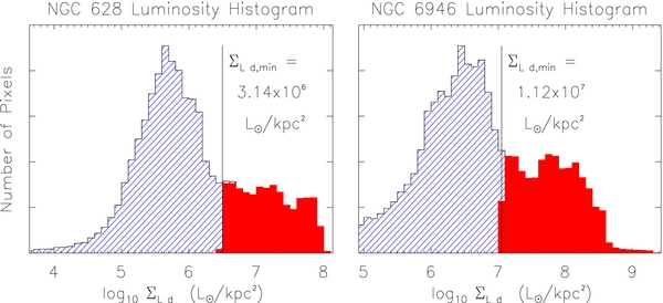
Figure 20. Dust luminosity surface density  histogram of a region containing NGC 628 (left) and NGC 6946 (right) shown in Figures 4 and 10. The modeling is done at MIPS160 resolution (18'' pixels) using all the cameras available. The shaded (red) area corresponds to the pixels identified as "galaxy pixels" in the galaxy mask. The line-shaded (blue) area corresponds to "non-galaxy pixels" (i.e., background pixels and other sources in the field not connected to the galaxies).
Download figure:
Standard image High-resolution imageAt this point, we have a well-determined separation of the image into (preliminary) "galaxy pixels" and the non-galaxy pixels. We now continue with steps 6–9, where we essentially repeat steps 2–5, starting with the PGM as our SNBM. The new masks generated in steps 6–9 are very similar to the corresponding ones previously generated on steps 2–5, with only small differences in the low surface brightness areas. The combined procedure is robust and precise.
- 6.For each band b, we obtain an Individual Background Mask (IBMb) with the iterative algorithm described in Appendix B. For this construction, we consider the pixels in the PGM as "non-background" pixels (i.e., they were not considered as background pixel candidates).
- 7.We construct a Background Mask (BM) using the same procedure as in step 3, but using the IBMbs instead of the PIBMbs.
- 8.Using the complement of the BM "non-background areas" and the algorithm described in Appendix B, we background subtract each individual image. The complement of BM masks all recognized sources in the background estimate for each individual image.
- 9.Using the background-subtracted images, we proceed to perform the final dust modeling at MIPS160 PSF using all the cameras available. We construct a Galaxy Mask (GM) in the same way as we constructed the PGM (using the same values of). The final GM and PGM will differ only in a few boundary pixels.

In G. Aniano et al. (2012, in preparation) the same masking method is applied to the full sample of 61 KINGFISH galaxies. Background companion galaxies are manually identified and removed from the masks when possible.
APPENDIX B: ALGORITHM FOR BACKGROUND RECOGNITION (IMAGE SEGMENTATION) AND SUBTRACTION
Given an image I expressed in its native pixel grid (x, y), and a (potentially empty) set NBStd of "non-background" sky regions expressed in a standard 4'' × 4'' grid (a grid common to all the images), we iteratively construct a sequence of "background" pixels masks Bn, n = 0, 1, 2, ..., and a sequence of tilted planes planen, n = 0, 1, 2, hellip; that approximate the image values over the sets Bn, n = 0, 1, 2, hellip;. The sets Bn, n = 0, 1, 2, hellip; will exclude the "non-background" NBStd regions, i.e., it is assumed that the pixels in NBStd are not background-candidate pixels.
Throughout the algorithm, the given "non-background" regions will be masked and not considered in the fitting. We start by bi-linearly interpolating or averaging (depending on the grid relative pixel sizes) the set NBStd into the image I grid (x, y) to obtain NBPrev.
We first smooth the original image by convolving it with a (normalized) Gaussian kernel ∝exp [ − (r/r0)2], with r0 equal to 0.56 times the width of the native pixel for each camera. The factor 0.56 is chosen so that each pixel contributes half of its flux to the corresponding pixel in the convolved image. This step provides a less noisy image, in which we can more robustly identify the galaxy and the external sources.
We proceed as follows. We start by setting B0 to be all pixels in the grid (x, y), except for the pixels in NBprev (if any). We fit a plane plane0 to the image values over the B0 pixels. This is achieved by finding the plane0 that minimizes 0 defined as
where n = 0. We compute the dispersion θ0 defined as
where n = 0, so the sum is over the B0 (original "background" candidate) pixels.
We take the first (n = 1) set of "background pixels"35 B1 to be all pixels that do not belong to NBprev, or lie more than κ θ0 above plane0 (κ is a constant, and we use κ ≡ 1.8, see below for details):
In the first step, these pixels typically correspond to the brightest point sources and central pixels of the galaxy.
We now proceed iteratively by
- 1.Fitting a tilted plane planen to all the candidate "background pixels" Bn, by minimizingn defined by Equation (B1).
- 2.Computing θn, defined by Equation (B2), where the sum extends over the Bn pixels.
- 3.Identifying a new set of "background pixels" Bn + 1 to be those pixels which lie inside the interval (planen − κ θn, planen + κ θn), and do not belong to NBprev:
This iteration will generate a sequence of tilted planes planen, and a (generally decreasing) set of "background pixels" Bn. The iteration will converge, i.e., it reaches a step M where BM + 1 = BM, typically in M = 20–250 iterations.
Once the iteration converges, we have set of "background pixels" BM, and a fitting plane planeM (all the computed sets Bn and planes planen will depend on the choice of κ, see below for a discussion). We bi-linearly interpolate or average BM to the standard 4'' × 4'' grid. This will generate a mask of the "background regions" in the standard grid, so it can be compared with the results of the algorithm from images of different cameras. We can generate standard mask of "non-background regions" by taking the complement of the "background regions" mask. The left columns of Figures 22 and 23 show the resulting residuals for NGC 628 and NGC 6946, respectively, over BM, for κ = 1.8. Rows 1–4 correspond to IRAC4.5, MIPS24, PACS160, and SPIRE350, respectively. It can be seen that the algorithm masks out all the point sources, extended sources, and several background regions. Residuals slightly positive are found in the edges of the extended emission areas, although most of the extended emission areas are recognized and excluded.
After the iteration converges to a set of "background pixels" BM, if we desire to perform a background subtraction to the images, we run the iterative steps again. In the second iteration, we use the original (non-smoothed) image, and the complement of the set BM found as the starting set of "non-background pixels" NBprev, i.e., the pixels which were recognized as having emission in the first iteration are masked out. The second run of the iteration will converge to a new set of "background pixels" BN, and a new fitting plane planeN, typically in N = 20–250 iterations. Clearly, by construction, we always have BN⊆BM. Finally, the last plane planeN is subtracted from I.
The reason to perform the second iteration, with the original image and a larger set of starting "non-background pixels," is that we can remove noisy pixels from the background pixels, recognize the edges of the emission areas more precisely, and perform a more precise background level estimation. Moreover, if we try to perform a single iteration (i.e., by going directly to the second iteration), then the larger image noise will prevent us from recognizing the dimmer sources and extended emission areas. The center columns of Figures 22 and 23 show the resulting residuals for NGC 628 and NGC 6946, respectively, over the sets BN.
It can be shown that if there exist an infinite set of background points B0 in which the intensities are independent noise drawn from a distribution with probability density ρ, then the algorithm will asymptotically converge:  , that will depend on κ. We define f(κ), the fraction of the original background-candidate pixels that are asymptotically considered background:

For noise distribution function densities ρ which are analytical around their expectation values, it can be shown that if  then Bn will converge to an empty set ∅; and Bn will converge to a non-empty set provided that
  , i.e.,
  . In particular, for a top hat distribution (ρ(x) = 1/2⇔|x| ⩽ 1), BN = B0 if
  , i.e.,
  . If the noise has a Gaussian distribution with standard deviation σ, we can numerically compute f(κ), and the actual σ/θ (the ratio between the distribution standard deviation σ and the computed final dispersion θ). Figure 21 shows the values of f(κ) (dotted green line) and θ/σ (solid blue line) for 1.6 < κ < 2.6 for a Gaussian distribution. The vertical red lines correspond to the threshold value
  , and the used value κ = 1.8.

Figure 21. Theoretical performance of the iterative algorithm for Gaussian random noise. The horizontal axis corresponds to the cutoff threshold κ. The dotted green line shows θ/σ, the ratio between the dispersion of the final set BN and the dispersion of the original distribution. The solid blue line shows the fraction of the original points that survive in BN. The vertical red lines correspond to the critical value  and the used value κ = 1.8.
Download figure:
Standard image High-resolution imageOur choice of κ is dictated by (1) the need to have  in order for the procedure to converge to a non-empty set, (2) the desire to minimize inclusion of outliers that may be due to rare events (e.g., cosmic rays, image artifacts), and (3) the desire to be as sensitive as possible to dim sources. We choose κ = 1.8 as a good compromise. If the background noise were Gaussian, for our choice κ = 1.8, we have f(κ = 1.8) = 0.5506, θ/σ = 0.4202 (i.e., the final iteration should fit only ≈55% of the background points, and their measured dispersion should be 0.4203σ).
How well does the iterative procedure behave with real images? Typically the iterative procedure converges in 20–250 steps. The right columns of Figures 22 and 23 show the resulting histograms of the background-subtracted intensities in BN for NGC 628 and NGC 6946, respectively. The solid red curve is a Gaussian distribution function with σ = θ/0.4202, i.e., with the standard deviation expected from the measured dispersion. The fit of the Gaussian curve to the histograms in Figures 22 and 23 is very good, supporting the validity of the presented algorithm.
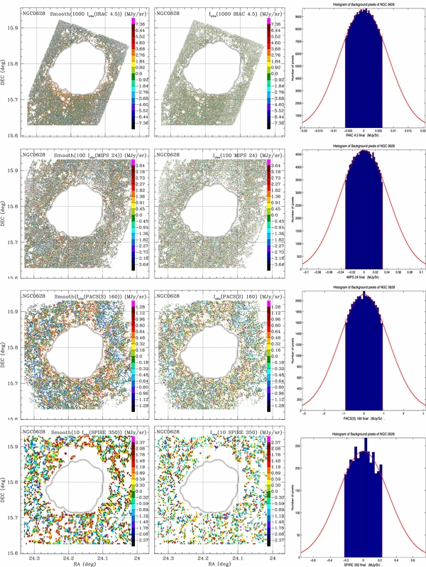
Figure 22. Analysis of the residuals in NGC 0628. Row 1: IRAC4.5. Row 2: MIPS24. Row 3: PACS160. Row 4: SPIRE350. Left column: residuals on the set BM (after the first iteration of the algorithm on the smooth image). Center column: residuals on the set BN (after the second iteration on the original image). Right column: histograms of the pixels on BN. The (red) solid line is a Gaussian with σ = θ/0.4202 (see the text for details).
Download figure:
Standard image High-resolution image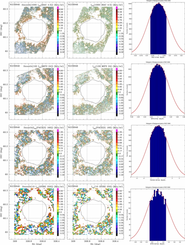
Figure 23. Same as Figure 22, but for NGC 6946. The bright carbon star V0778 Cyg, located near R.A. = 309.044, decl. = 60.082 (slightly off the bottom left edge of the maps shown) produces strong artifacts in the IRAC and MIPS cameras, reducing the useful background area of the images.
Download figure:
Standard image High-resolution imageThis background recognition algorithm has several advantages over other approaches. First, the algorithm is very robust, automatic, and quick, and produces superior results when dealing with all the ≈1400 images of the KINGFISH sample. Second, by keeping only a subset (≈ 55%) of the background pixels, the last computed dispersion is small enough that even dim sources are easily recognized and masked. This allows us to exclude virtually all detectable foreground or background sources from the subset of points used to determine the background of the images. Third, this algorithm also recognizes areas with dim extended emission. Fourth, image artifacts over the background areas are easily identified, allowing us to minimize bias induced by them in the background estimation. This allows us to avoid over- or under-subtraction of the background in each image, which is critical in order to model the galaxy low surface brightness areas. Table 5 summarizes the background and image information for the different cameras.
Table 5. Background Information for the Different Cameras
| NGC 0628 | NGC 6946 | |||||||
|---|---|---|---|---|---|---|---|---|
| Camera | Background Area | Image | Background Area | Image | ||||
| No. of | Percentb | σc | Max. | No. of | Percentb | σc | Max. | |
| Pixelsa | (%) | (MJy sr−1) | (MJy sr−1) | pixelsa | (%) | (MJy sr−1) | (MJy sr−1) | |
| IRAC3.6 | 234851 | 29.7 | 0.0052 | 160 | 291159 | 30.4 | 0.0093 | 183 |
| IRAC4.5 | 253580 | 31.1 | 0.0083 | 152 | 267213 | 28.2 | 0.0093 | 232 |
| IRAC5.8 | 260864 | 32.6 | 0.0285 | 59.6 | 301640 | 31.5 | 0.0274 | 617 |
| IRAC8.0 | 264790 | 32.6 | 0.0350 | 50.9 | 286791 | 30.3 | 0.0356 | 1441 |
| MIPS 24 | 124131 | 36.8 | 0.0432 | 88.0 | 87694 | 34.1 | 0.0328 | 2192 |
| MIPS 70 | 14264 | 41.1 | 0.439 | 70.9 | 8632 | 35.1 | 0.334 | 1645 |
| MIPS 160 | 3059 | 31.7 | 0.396 | 79.9 | 2996 | 40.8 | 1.02 | 715 |
| PACS(H)70 | 315588 | 43.3 | 4.55 | 605 | 231316 | 42.7 | 4.50 | 24106 |
| PACS(H)100 | 311051 | 42.7 | 4.40 | 635 | 226840 | 42.5 | 4.28 | 20227 |
| PACS(H)160 | 36836 | 45.3 | 2.35 | 226 | 264298 | 49.0 | 3.12 | 7090 |
| PACS(S)70 | 155675 | 40.1 | 2.50 | 590 | 126604 | 40.7 | 2.52 | 23115 |
| PACS(S)100 | 104132 | 39.5 | 2.30 | 506 | 82813 | 39.3 | 2.22 | 19275 |
| PACS(S)160 | 51115 | 39.3 | 1.25 | 237 | 34252 | 44.3 | 1.53 | 7439 |
| SPIRE250 | 7433 | 32.8 | 0.499 | 76.9 | 7393 | 40.9 | 0.873 | 1584 |
| SPIRE350 | 3306 | 39.8 | 0.303 | 21.7 | 2470 | 38.1 | 0.392 | 358 |
| SPIRE500 | 1230 | 29.5 | 0.122 | 6.92 | 1151 | 33.7 | 0.186 | 84.1 |
Notes. aNumber of native pixels that are considered "background." bPercent of the non-galaxy pixels that are considered "background" pixels. cStandard deviation of the Gaussian fit of the "background" pixels.
Download table as: ASCIITypeset image
APPENDIX C: CORRECTION FOR MISSING DATA (BAD PIXELS) IN THE ORIGINAL IMAGES
Some of the original images include bad pixels due to detector saturation, incomplete scanning, or other problems. This effect is not important when present in the pixels far away from the target galaxy, but may have undesired consequences if not treated appropriately when present near or within the target galaxy. A similar situation arises when observations are made over a small part of a galaxy, for example, with the IRS instrument on board the Spitzer Space Telescope. We develop a method for correcting this problem.
In order to estimate (and correct) the influence of bad pixels of a camera A, we start by choosing a second camera B. We require that the sky coverage of camera B be larger than camera A, or at least that does not present bad pixels in the same areas as A. From all the possible candidates for being the correcting camera B, we choose the camera with wavelength most similar to A. For example, we typically correct the MIPS160 camera with the SPIRE250 camera.36
We divide the original image grid of the camera A, OGA, into two sets of pixels: OGA, good, the pixels of OGA with good A data, and OGA, bad, the pixels of OGA in which the camera A has bad data.
We interpolate the background-subtracted image B from its original grid OGB into the OGA grid, obtaining Binterp A, which looks morphologically similar to A. We construct two images Bgood and Bbad, both defined on OGA, as follow:
We process the images Bgood and Bbad exactly as we do with the image A; we rotate them, convolve with the kernel that corresponds to the image A, and interpolate them to the final grid (FG). A given output pixel in FG will have flux fluxgoodB, and fluxbadB in the final stage of processing the Bgood and Bbad images, respectively. We define FA, B(x, y) ∈ FG, the fraction of the total flux in the FG coming from areas with good A data, as

FA, B provides an estimate of how much flux we are missing in each output pixel due to the missing data in the original image A. In the pixels for which FA, B > 0.65 (i.e., those where most of the flux is actually coming from regions where we know A) we can further compensate the final stage of the A image processing by multiplying the value obtained by 1/F. In the points FA, B < 0.65 a significant amount of the flux (more than 35%) is coming from regions where A is not known, so we mask and ignore them.
This correction algorithm would be exact if the color A/B were constant, and the PSFs of both cameras coincided. We test the algorithm by purposely removing some part of an image, and correcting it with itself or another image. In the former case, the results are exact within numerical noise. In the latter case, because we are correcting an image A with a different one B, the method is not exact, but in most cases still provides a quite accurate result.
APPENDIX D: UNCERTAINTY ESTIMATES IN COMMON-RESOLUTION IMAGES
The χ2 maps also shed light on the estimated flux uncertainties. The value of
depends not only on the ability of the model to fit the data, but also on the adopted uncertainties  . For a given data set and fitted model, underestimation of the uncertainties
  would lead to higher vales of χ2. Recall that the
  were estimated by studying the pixel-to-pixel variations in the background regions outside the galaxy mask. If part of the background variations actually comes from real variations in emission from foreground dust, or dusty background galaxies, then our dust model procedure may actually be able to partially fit the background variations, leading to a low value of χ2. On the other hand, image artifacts and departures of the real data from the models will lead to higher values of χ2. It is clear, for example, that the differences in the PACS and MIPS photometry must lead to an increase in the χ2 values, since the model cannot fit simultaneously two different flux values.
If we have N measures from an ideal model with M adjustable parameters, each measure having independent Gaussian noise with variance  , then the χ2 of the fit will have a chi-square distribution with degrees of freedom (dof), where dof = N − M. The χ2/dof map will have mean 1, and dispersion
  .
.
In our background noise estimation procedure, after we recognize and mask all the background sources and subtract a "tilted plane," in each image there remains a zero-mean background due to unresolved dim sources. We use the dispersion of the background pixels (with respect to the best-fit plane) to estimate the stochastic background uncertainty. This provides a valid uncertainty estimate since the same background structures will be present over the galaxy, so our galaxy fluxes will be uncertain (at least) at this level. However, this background dispersion is not only due to random noise in the detectors, it also includes a contribution from foreground and background sources. Figure 24 shows the correlation of the dispersion of the background pixels from the MIPS160 (horizontal axis) and SPIRE350 (vertical axis) cameras. Although the residual distributions have zero mean, there is a strong correlation between the MIPS160 and SPIRE350 flux in the background pixels, demonstrating a component coming from real astrophysical sources. Other cameras show similar correlations. The modeling can fit these correlated departures from zero by adding positive or negative amounts of real dust, reproducing the departures and therefore decreasing the χ2 of the fit. We therefore expect to have χ2/dof < 1 in areas where the flux uncertainties have an important contribution from unresolved dim sources (i.e., in the background pixels or low surface brightness areas).
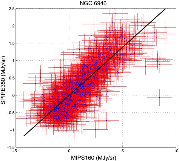
Figure 24. Background-subtracted intensities in the MIPS160 and SPIRE350 cameras, for background pixels around NGC 6946. There is a strong correlation between the MIPS160 μm and SPIRE350 μm fluxes, indicating that the dispersion has a component coming from unresolved dim astrophysical sources.
Download figure:
Standard image High-resolution imageFigure 25 shows the contribution of different cameras to χ2 for NGC 628. The fit is done at MIPS160 resolution, using all 13 cameras available. We employ the recommended dust model with six adjusted parameters (Ω⋆, Mdust, qPAH, γ, Umin, α) leading to a fit with dof = 7. The upper left panel (a) shows the χ2/dof map. If the data were artifact-free, perfectly modeled, with independent Gaussian noise, the map would have mean 1, and dispersion  . The actual χ2/dof values are slightly above 1 in the bright regions and below 1 in the outer parts of the galaxy. In the outer parts of the galaxies, the correlation of the noise between the cameras drives the χ2/dof below the expected value 1. In the bright spots of the galaxy, the differences in PACS and MIPS photometry decrease the quality of the fit. We estimate the PACS and MIPS photometry uncertainties in a way that their contribution to the χ2 maps is controlled and consistent, but the model will try to fit some intermediate (probably non-physical) value which may impair its ability of accurately fitting the remaining cameras.
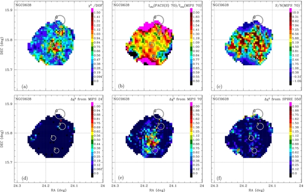
Figure 25. Analysis of the χ2 contributions for NGC 628. The fit is done at MIPS160 resolution, using all 13 cameras with 6 adjusted parameters (Ω⋆, Mdust, qPAH, γ, Umin, α). Top left panel: χ2/dof map. Top center panel: PACS70/MIPS70 ratio map. Top right panel: estimated S/N map for MIPS70. The lower row shows the contribution Δχ2 of selected cameras to the total χ2: left panel shows MIPS24 camera, center panel MIPS70, and right panel shows SPIRE350. The Δχ2 behaves as expected.
Download figure:
Standard image High-resolution imageIn order to remedy this situation, uncertainties for the PACS and MIPS photometry are estimated by comparing the PACS and MIPS images (see below). The uncertainties are slightly overestimated, thus giving more weight to the remaining artifact-free cameras. Figure 25(b) shows the PACS(S)70/MIPS70 ratio map. Stripes aligned with the MIPS sky scanning directions near the galaxy center suggest the presence of MIPS image artifacts. Discrepancies in the low surface brightness areas (outer parts of the galaxy) suggest differences in the ability of the telescopes to measure the low surface brightness areas correctly. The top right panel (c) shows the assigned MIPS70 S/N map. The procedure described in Appendix D.1 assigns large uncertainties to the areas where the PACS and MIPS images have discrepancies, leading to reduced S/N. This is a critical step toward getting χ2 maps that really measure the goodness of the model fit, not only the data discrepancies.
The lower row of Figure 25 shows the contribution Δχ2 of selected cameras to the total χ2 for NGC 628. The lower left panel (d) shows the contribution of MIPS24 camera. We note that this contribution is extremely low, under 0.05 for most of the galaxy. This is because the dust model can adjust the 24 μm flux relatively independently of the other observed bands by adjusting γ and α. The 24 μm band is unique in lying a factor of three in wavelength away from the nearest other bands (8 μm and 70 μm). Figure 25(e) is the contribution of MIPS70 μm to the total χ2. Even though the MIPS70 camera has severe artifacts, its Δχ2 near the center is controlled by the large values of σ assigned. Figure 25(f) shows Δχ2 for SPIRE350. The camera behaves exactly as expected, contributing Δχ2 ≈ 0.6 near the galaxy nucleus and smaller Δχ2 in the low surface brightness areas. The behavior for NGC 6946 is similar.
D.1. Uncertainty Estimate Procedure
In order to estimate uncertainties for the different cameras, we proceed as follows.
For each camera of wavelength λk, after the image processing (rotation to R.A.–decl., background subtraction, convolution to a common PSF, correction for boundary effects and missing data, and resampling to the FG) the flux in each final pixel is a (known) linear combination of the flux of (in principle) all the original pixels of the camera. If the statistical properties of the uncertainties in the original pixel fluxes were known, it would be possible to infer the uncertainties (and their statistical properties) in each final pixel. The original maps oversample the beam, and have artifacts that extend over several pixels, so realistic statistical properties of the uncertainties are difficult to determine. We therefore estimate the uncertainties directly in the final (post-processed) image.
We always assume that the pixel noise is not correlated between different cameras, so in what follows we work in each image independently, and omit the subindex identifying the camera in the following discussion. For each pixel, we will consider two independent sources of uncertainties δsto and δsys. The term δsto will be the uncertainty due to stochastic pixel noise and the existence of (unresolved) background dim sources. We estimate it by measuring the flux fluctuations in the background pixels. The term δsys will include systematic and calibration uncertainties.
In order to estimate the term δsto, the stochastic pixel noise, we proceed as follows. We re-grid the BM to the final-map grid to define a set of Nbg "background pixels." For each camera k, we compute the background dispersion  as
as
where  is the background-subtracted flux of the camera of wavelength λk in the pixel (x, y) in the last stage of the image processing (i.e., after the image has been rotated to R.A.–decl., background plane subtracted, convolved to a common PSF, corrected for boundary effects and missing data, and resampled to the FG). The background dispersion
  includes the propagation of original pixel noise and artifacts into the background pixels, possible non-ideal background subtraction and the contributions of unidentified faint background sources.
  does not contain information on the correlation of the noise among the different pixels or calibration uncertainties.
For each camera, we consider the pixel-dependent uncertainty δsys, j as

where is the calibration uncertainty for the camera; K is 0 for IRAC, MIPS24, and SPIRE cameras and an estimate of systematic uncertainties for MIPS70,160 and PACS cameras (where such estimation is possible). The main difficulty in estimating is that the cameras are typically calibrated using point sources. We are performing resolved studies of an extended sources, so we have additional uncertainties due to the extended source corrections.
For the IRAC cameras, the standard calibration uncertainty is = 0.05 for point sources (Dale et al. 2005), but we will adopt a larger value to account for the uncertainties in the extended emission correction. The IRAC images are calibrated for point sources. We multiplied the intensities by the asymptotic (infinite radii) value of the aperture correction factors C = 0.91, 0.94, 0.66, 0.74 for the 3.6 μm, 4.5 μm, 5.8 μm, and 8.0 μm bands, respectively. This correction would lead to a correctly calibrated image if the source had constant surface brightness. Since galaxies contain nonuniform emission, the aperture correction factor should, in principle, be different in each region. We multiply the entire image by the factors C, and arbitrarily assign 1/3 of the correction as uncertainty. We use = 0.05 + 1/3 × (1/C − 1) = 0.083, 0.071, 0.221, 0.167 for the 3.6 μm, 4.5 μm, 5.8 μm, and 8.0 μm bands, respectively. These corrections will overestimate the uncertainties in the diffuse regions and underestimate the uncertainties near bright point sources.
For the MIPS, PACS, and the SPIRE cameras we adopt = 0.10. This value is larger than the estimated 4% calibration uncertainty for point sources for MIPS24 (Engelbracht et al. 2007), ≈4% for PACS (Müller et al. 2011), and 7% for SPIRE,37 and comparable to estimates for MIPS70 (Gordon et al. 2007) and MIPS160 (Stansberry et al. 2007). For the MIPS70,160 and PACS cameras, however, δsys will be dominated by K in most of the pixels.
For MIPS70 and MIPS160, we can estimate the systematic uncertainties K by comparing the PACS and MIPS resolved photometry. In most of the pixels, the observed differences are larger than expected due to the differences in the camera spectral responses or calibration uncertainties. For PACS70 and PACS160 we can estimate the systematic uncertainties K by comparing the PACS and MIPS resolved photometry For the PACS100 camera we can estimate the systematic uncertainties K by extrapolating the uncertainties estimated for the PACS70 and PACS160 cameras. We proceed as follows.
D.1.1. Systematic Uncertainties for MIPS70 and MIPS160 Cameras
Since for the 70 μm and 160 μm bands the PACS FWHM are smaller than the corresponding MIPS FWHM (see Table 1), in all the common-PSF maps where we employ MIPS data we have PACS data as well. Therefore, we can compare PACS and MIPS images after the image processing. The comparison is straightforward since both images are in the same final-map grid and PSF.
We consider the difference

where IobsMIPS, j and IobsPACS(S), j are the observed MIPS and PACS (Scanamorphos) flux, in the same band (70 μm or 160 μm). We consider the Scanamorphos data reduction more reliable than the HIPE, so we only employ the Scanamorphos images in the PACS–MIPS comparison. The term DPM, j captures both image artifacts and differences in camera performance and calibration. Unfortunately, artifacts in the PACS cameras will induce uncertainties in the MIPS fluxes and vice versa, but there is no robust, automatic way of isolating the image artifacts. We take

D.1.2. Systematic Uncertainties for PACS70 and PACS160 Cameras
Based on our dust modeling, we consider the Scanamorphos data reduction to be more reliable than the HIPE-only data reduction. When the MIPS and PACS cameras for a band (70 μm or 160 μm) are used in a final-map PSF (e.g., MIPS70 and PACS70 can be used if the final-map PSF is SPIRE350, SPIRE500, or MIPS160) we proceed in a similar way as for the MIPS bands, taking

When the MIPS camera for a band (70 μm or 160 μm) is not used in a given final-map PSF (e.g., MIPS70 cannot be used if the modeling is done at PACS160 PSF), the comparison between PACS and MIPS is more complex. We start by convolving the PACS image into the corresponding MIPS PSF, and re-binning it into the MIPS native pixel grid, denoted as IobsPACS@M. We can compare IobsPACS@M and IobsMIPS since both images are expressed at the same grid and have the same PSF. We construct PM, the fractional PACS–MIPS difference (with respect to the PACS image), at the MIPS PSF, as
We re-bin PM into the final-map grid, and we take

where J is the pixel in the PACS@M image grid that contains pixel j. This procedure produces an uncertainty image EPM, j at the final-map grid and PSF, that if degraded into the corresponding MIPS PSF would be ∼|IobsPACS(S)@M − IMIPSobs|. In this situation, we finally take

D.1.3. Systematic Uncertainties for PACS100 Camera
In the case of PACS100, we do not have any other camera available to perform a direct comparison. We therefore estimate the uncertainties by extrapolating the uncertainties previously calculated for PACS70 and PACS160 as follows. We therefore will assume

where
Figure 26 shows the resulting S/N estimates for MIPS70 and PACS70 observations of NGC 6946.

Figure 26. 70 μm images of NGC 6946 convolved into MIPS160 PSF. Left: map of PACS70/MIPS70. Center: S/N map of MIPS70. Right: S/N map of PACS70. The image artifact that extends from the galaxy nucleus toward the west northwest induces a low S/N area in the cameras. This artifact, aligned with the MIPS sky scanning direction, is probably due to saturation, latency or nonlinearities in the MIPS detector. In other areas with PACS70/MIPS70  it is not clear which camera is responsible for the bad behavior.
Download figure:
Standard image High-resolution imageAPPENDIX E: UNCERTAINTY ESTIMATES FOR MODEL PARAMETERS
In order to estimate the model parameter uncertainties, we generate a set r = 1, 2, ..., Nr realizations  including random noise, for each pixel j, modeling the noise
  in pixel j as a sum of three components:

 represents the non-correlated noise component of the pixel j, while
  and
and  represent the correlated noise component and systematic/calibration uncertainties, assumed to be (completely) correlated among the different pixels of the camera.
  is drawn from an independent Gaussian distribution for each pixel, while
  and
and  are drawn from a global Gaussian distribution, properly normalized for each pixel.
For each camera, we generate a set of N × Nr "pixel" Gaussian variables, with zero mean and variance 1, ηj, r, j = 1, 2, ...N, r = 1, 2, ..., Nr, where N is the total number of pixels in the image, and a set of 2Nr "global" Gaussian variables, with zero mean and variance 1,  .
.
We set


where  and
and  were defined by Equations (D2) and (D3). The division of the dispersion
  into equal correlated and uncorrelated components
  and
and  is arbitrary, but seems to capture the main features of the noise. A more sophisticated treatment would use the statistic of the background region to characterize the correlation of the noise in pixels as a function of their separation, but this is beyond the scope of the present work.
For each pixel, the 1σ uncertainty in the measured flux density  used to calculate the χ2j of the model (see Equation (13)) is given by
Uncertainties for the inferred (pixel) model parameters are computed using Equation (28). In order to compute the uncertainties in the global quantities, we use Equation (28) on the global quantities, i.e., for each random realization we compute the global inferred quantity and finally we compute the dispersion on the inferred global quantities. This approach preserves the correlation in the pixel noise consistently into the global uncertainties.
APPENDIX F: INSTRUMENT COMPARISON: PACS–MIPS PHOTOMETRY DISAGREEMENT
In Section 7 we show that maps made at PACS160 resolution (using IRAC, MIPS24, and PACS data only) are less reliable. Furthermore, maps using IRAC and PACS data at MIPS160 resolution provide less accurate38 results than maps computed with IRAC and MIPS data using the same PSF. We therefore proceed to analyze the differences in the PACS and MIPS photometry, to shed light onto the roots of such discrepancies.
Figures 27 and 28 compare the two different PACS data reduction schemes (Scanamorphos and HIPE) with the MIPS camera for NGC 628 and NGC 6946, respectively. All images were convolved into a Gaussian PSF with 64'' FWHM, a PSF broad enough that any camera PSF mismatch should not produce any artifact. The left column shows the PACS/MIPS ratio maps over the galaxy mask. The center columns show an intensity–intensity scatter plot for the galaxy pixels (the pixels in the left column). The right column has a zoom of the −5–30 MJy sr−1 region of the center column plots. We compare PACS70 Scanamorphos and MIPS70, PACS70 HIPE, and MIPS70, PACS160 Scanamorphos and MIPS160, and PACS160 HIPE and MIPS160. In the center and right column, the horizontal and vertical red lines correspond to the 1σ error estimates. By the inclusion of the PACS(S)–MIPS difference term in the uncertainty estimates (see Appendices D.1.1 and D.1.2), the 1σ error estimates will intersect the PACS=MIPS line.

Figure 27. Comparison of the different 70 μm and 160 μm data available for NGC 628, after background subtraction, and convolved into a Gaussian PSF with 64'' FWHM. The left column shows the PACS–MIPS ratio maps over the galaxy mask. The center column shows scatter plot of the camera intensity of the galaxy pixels. The right column is a zoom of the −5–30 MJy sr−1 region of the center column plots. Top row: PACS70 Scanamorphos and MIPS70. Second row: PACS70 HIPE and MIPS70. Third row: PACS160 Scanamorphos and MIPS160. Bottom row: PACS160 HIPE and MIPS160. The ratio maps show strong discrepancies in the three data sets (i.e., the band ratios differ from ≈1 in most of the galaxy).
Download figure:
Standard image High-resolution image
Figure 28. Same as Figure 27, but for NGC 6946.
Download figure:
Standard image High-resolution imageThe Scanamorphos and HIPE pipelines give similar results in the high surface brightness areas, having slightly larger intensities than MIPS (see Figures 27 and 28). The main difference between the two data reduction schemes is in the low surface brightness areas: Scanamorphos intensities are larger than HIPE intensities.
Even though the PACS and MIPS cameras have different spectral response, smooth spectra appropriate to star-forming galaxies should result in nearly the same measured intensity for both MIPS70 and PACS70, and likewise for MIPS160 and PACS160. For our best-fit SEDs for NGC 628 and NGC 6946, we expect PACS70/MIPS70 ∼1.085, and PACS160/MIPS160 ∼1.022 (see Table 6). However, the measured PACS global flux densities do not agree so well with MIPS values, as seen in Table 6. The situation is more critical in resolved studies. Even though the global PACS and MIPS fluxes agree within ≈20%, the ratio maps shows strong discrepancies in the three data sets: the band ratios differ from ≈1 in most of the galaxy.
Table 6. PACS70/MIPS70 Flux Ratio Predicted by the Model and Observed
| NGC 628 | NGC 6946 | |||
|---|---|---|---|---|
| Band Ratio | Model | Observed | Model | Observed |
| PACS(H)70/MIPS70 | 1.083 | 0.919 | 1.088 | 1.040 |
| PACS(S)70/MIPS70 | 1.083 | 1.243 | 1.088 | 1.246 |
| PACS(H)160/MIPS160 | 1.024 | 0.886 | 1.020 | 1.016 |
| PACS(S)160/MIPS160 | 1.024 | 1.058 | 1.020 | 1.252 |
Download table as: ASCIITypeset image
Figure 29 shows the 70 μm/160 μm color inferred from the different data sets. Again, all images were convolved into a Gaussian PSF with 64'' FWHM. The top row corresponds to NGC 628 and the bottom row to NGC 6946. The left column is the PACS-Scanamorphos color, PACS HIPE is shown in the center column, and, MIPS is shown in the right column. The 70 μm/160 μm colors inferred with the different cameras are also quite different, especially in the outer parts of the galaxies.
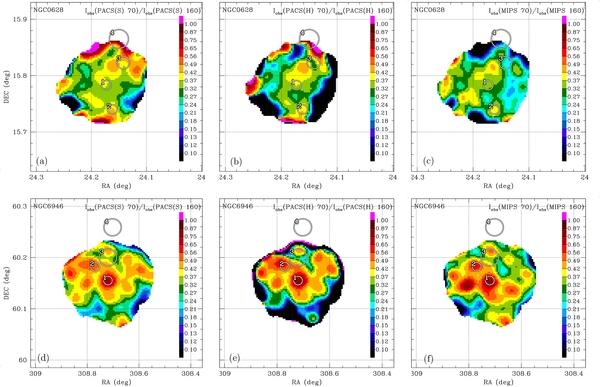
Figure 29. Comparison of the 70 μm/160 μm color inferred from the different data sets. All images were previously convolved into a Gaussian PSF with 64'' FWHM. The top row corresponds to NGC 628 and the bottom row to NGC 6946. Left column: PACS-Scanamorphos color. Center column: PACS HIPE. Right column: MIPS. The 70 μm/160 μm colors inferred with the different cameras are quite different, especially in the outer parts of the galaxies.
Download figure:
Standard image High-resolution image
The colors inferred from PACS(S)70/PACS(S)160 and MIPS70/MIPS160 are similar for most of the galaxy, and thus the inferred dust parameters (Umin) obtained at PACS160 resolution are similar to the ones obtained at MIPS160 resolution. The large PACS(S)160/MIPS160 flux ratio makes the modeling at PACS160 resolution add more dust over all the galaxy, compared to our modeling at MIPS160 resolution, when MIPS constraints are present.
The colors inferred from PACS(H)70/PACS(H)160 and MIPS70/MIPS160 are very different in the outer parts of the galaxy, potentially giving different best-fit parameters in the dust modeling. The HIPE pipeline uses a high-pass filter in the time line observing series before constructing the two-dimensional image map. In studies of HIPE performance using simulated data with realistic noise statistics, it was shown that HIPE intensities are always equal to or smaller than the "true" intensities in the extended low surface brightness regions (M. Sauvage 2011, private communication). When only one SPIRE band (SPIRE250) is included, then the extremely low flux of PACS(H)160 in the low surface brightness regions of the galaxy makes the dust appear to be very cold, and thus increases the amount of dust needed to reproduce the SPIRE250 flux in those regions. We therefore do not recommend to use the HIPE data reduction pipeline for the PACS cameras.
We do not recommend working at PACS160 resolution, unless there is reason to think that high S/N has been achieved. We note, however, that even in regions of moderately high surface brightness, the PACS and MIPS photometry often disagree at the 30% level (see Figures 27 and 28), making dust modeling risky if PACS provides the only data longward of 24 μm. If SPIRE250 data are available, dust modeling can be done at SPIRE250 resolution with results that are reasonably reliable. We note in Figure 14 that total dust masses obtained using IRAC, MIPS24, PACS, and SPIRE250 as constraints are in error by only ≈35%, provided the PACS-Scanamorphos data are used.
We further note that NGC 6946 is a particularly challenging galaxy to model: it has over four decades of dynamic range in the PACS160 band, including an extremely high surface brightness nucleus.
Footnotes
- 18
Photometry at 850 μm was available for 26 galaxies in the SINGS sample, but the data were only reliable (and used) for 17 galaxies.
- 19
For example, the 70 μm and 100 μm channels of the PACS instrument use the same optical path in the telescope, but differ in the filter used, and thus have different PSFs, so we will consider them as different "cameras."
- 20
Details can be found in the data release documentation, http://data.spitzer.caltech.edu/popular/sings/20070410-enhanced-v1/Documents/sings-fifth-delivery-v2.pdf
- 21
- 22
Details can be found in the data release documentation, http://data.spitzer.caltech.edu/popular/lvl/20090227-enhanced/docs/LVL-DR3-v1.pdf
- 23
- 24
Table 4 of Aniano et al. (2011) quantifies the corresponding PSF mismatch: all the kernels employed have D < 0.064.
- 25
Draine et al. (2007) in a global study of 61 galaxies in the SINGS sample found a median value of qPAH = 0.034.
- 26
In our modeling, we find best-fit qPAH < 0.05 for virtually all of the galaxy pixels, compatible with the average observed 2175 Å feature in local diffuse clouds, i.e., models with qPAH > 0.05 are not needed, except for error estimation.
- 27
The mean stellar brightness emerging from each pixel is not the same as the starlight intensity seen by the dust grains, and therefore we do not expect a tight correlation between the dust heating and Ω⋆.
- 28
We employ the appropriate spectral response function for each camera. For SPIRE, we use the spectral response functions appropriate for extended sources, as described in the SPIRE observers' manual.
- 29
We try log10Umax ∈ {3, 4, 5, 6, 7, 8}.
- 30
In some regions where we do not have complete data coverage or the S/N is low, we may further fix some of the parameter values. This situation typically arises in background areas without IRAC coverage, in which case we fix Ω⋆ = 0.
- 31
We do not use the median maps that could be constructed from modeling adding random noise to the observations to estimate the parameter uncertainties.
- 32
We take global photometry to be the photometry within the galaxy mask, i.e., the galaxy regions where we can reliably determine the dust luminosity. There is undoubtedly additional emission from material outside the galaxy mask, but it cannot be measured reliably.
- 33
Even though MIPS160 PSF is our lowest resolution modeling, PACS–MIPS discrepancies made it important to be able to retain the MIPS160 camera in the modeling, and, as shown in Section 8, using lower angular resolution does not introduce a major bias in the modeling.
- 34
"Non-background" areas will include the target galaxy, and any other recognizable emission structures in the field.
- 35
"Background pixels" consist of pixels that are not part of the target galaxy, and any other recognizable emission structures (e.g., background galaxies) in the field, removing also any pixels that are "outliers," either above or below the general background.
- 36
We avoid correcting the MIPS160 camera with the PACS160 camera due to the inability of PACS160 camera to correctly measure the flux in extended emission regions. Moreover, the SPIRE maps extend to a larger area than the PACS maps.
- 37
See the SPIRE Observers' Manual HERSCHEL-DOC-0798, version 2.4.
- 38
That is, the resulting dust/H mass ratios seem less "reasonable."