


ABSTRACT
We present the results of a search for gravitational waves associated with 154 gamma-ray bursts (GRBs) that were detected by satellite-based gamma-ray experiments in 2009–2010, during the sixth LIGO science run and the second and third Virgo science runs. We perform two distinct searches: a modeled search for coalescences of either two neutron stars or a neutron star and black hole, and a search for generic, unmodeled gravitational-wave bursts. We find no evidence for gravitational-wave counterparts, either with any individual GRB in this sample or with the population as a whole. For all GRBs we place lower bounds on the distance to the progenitor, under the optimistic assumption of a gravitational-wave emission energy of 10−2 M☉ c2 at 150 Hz, with a median limit of 17 Mpc. For short–hard GRBs we place exclusion distances on binary neutron star and neutron-star–black-hole progenitors, using astrophysically motivated priors on the source parameters, with median values of 16 Mpc and 28 Mpc, respectively. These distance limits, while significantly larger than for a search that is not aided by GRB satellite observations, are not large enough to expect a coincidence with a GRB. However, projecting these exclusions to the sensitivities of Advanced LIGO and Virgo, which should begin operation in 2015, we find that the detection of gravitational waves associated with GRBs will become quite possible.
Export citation and abstract BibTeX RIS
1. INTRODUCTION
Gamma-ray bursts (GRBs) are intense flashes of γ-rays which are observed approximately once per day and are isotropically distributed over the sky (see, e.g., Mészáros 2006, and references therein). The variability of the bursts on timescales as short as a millisecond indicates that the sources are very compact, while the identification of host galaxies and the measurement of redshifts for more than 200 bursts have shown that GRBs are of extragalactic origin.
GRBs are grouped into two broad classes by their characteristic duration and spectral hardness (Kouveliotou et al. 1993). Long GRBs (≳2 s, with softer spectra) are related to the collapse of massive stars with highly rotating cores (see, e.g., the reviews by Modjaz 2011; Hjorth & Bloom 2011). The extreme core-collapse scenarios leading to GRBs result in the formation of a stellar-mass black hole with an accretion disk or of a highly magnetized neutron star; for a review see Woosley (2011) and references therein. In both cases the emission of gravitational waves (GWs) is expected, though the amount of emission is highly uncertain.
The progenitors of most short GRBs (≲2 s, with harder spectra) are widely thought to be mergers of neutron-star–neutron-star or neutron-star–black-hole binaries (see, e.g., Eichler et al. 1989; Narayan et al. 1992; Nakar 2007; Gehrels et al. 2009), though up to a few percent may be due to giant flares from a local distribution of soft-gamma repeaters (Duncan & Thompson 1992; Tanvir et al. 2005; Palmer et al. 2005; Nakar et al. 2006; Frederiks et al. 2007; Mazets et al. 2008; Chapman et al. 2009; Hurley et al. 2010). The mergers, referred to here as compact binary coalescences, are expected to be strong GW radiators (Thorne 1987). The detection of GWs associated with a short GRB would provide direct evidence that the progenitor is indeed a compact binary. With such a detection it would be possible to measure component masses (Finn & Chernoff 1993; Cutler & Flanagan 1994) and spins (Poisson & Will 1995), constrain neutron-star equations of state (Vallisneri 2000; Flanagan & Hinderer 2008; Hinderer et al. 2010; Read et al. 2009; Lackey et al. 2012; Pannarale et al. 2011), test general relativity in the strong-field regime (Will 2005), and measure calibration-free luminosity distances (Schutz 1986; Chernoff & Finn 1993; Dragoljub 1993; Dalal et al. 2006; Nissanke et al. 2010), which allow the measurement of the Hubble expansion and dark energy.
Several searches for GWs associated with GRBs have been performed using data from LIGO and Virgo (Abbott et al. 2005, 2008b; Acernese et al. 2007, 2008). Most recently, data from the fifth LIGO science run and the first Virgo science run were analyzed to search for coalescence signals or unmodeled GW bursts associated with 137 GRBs from 2005–2007 (Abbott et al. 2010b, 2010a). No evidence for a GW signal was found in these searches. For GRB 051103 and GRB 070201, short-duration GRBs with position error boxes overlapping, respectively, the M81 galaxy at 3.6 Mpc and the Andromeda galaxy (M31) at 770 kpc, the non-detection of associated GWs ruled out the progenitor object being a compact binary coalescence in M81 or M31 with high confidence (Abbott et al. 2008a; Abadie et al. 2012b).
Although it is expected that most GRB progenitors will be at distances too large for the resulting GW signals to be detectable by LIGO and Virgo (Berger et al. 2005), it is possible that a few GRBs could be located nearby. For example, the smallest observed redshift to date of an optical GRB afterglow is z = 0.0085 (≃ 36 Mpc) for GRB 980425 (Galama et al. 1998; Kulkarni et al. 1998; Iwamoto et al. 1998); this would be within the LIGO–Virgo detectable range for some progenitor models. Recent studies (Soderberg et al. 2006; Chapman et al. 2007; Le & Dermer 2007; Liang et al. 2007; Virgili et al. 2009) indicate the existence of a local population of under-luminous long GRBs with an observed rate density approximately 103 times that of the high-luminosity population. Also, observations suggest that short-duration GRBs tend to have smaller redshifts than long GRBs (Guetta & Piran 2005; Fox et al. 2005), and this has led to fairly optimistic estimates (Abadie et al. 2010; Leonor et al. 2009) for detecting associated GW emission. Approximately 90% of the GRBs in our sample do not have measured redshifts, so it is possible that one or more could be much closer than the typical ∼Gpc distance of GRBs.
In this paper, we present the results of a search for GWs associated with 154 GRBs that were detected by satellite-based gamma-ray experiments during the sixth LIGO science run and second and third Virgo science runs, which collectively spanned the period from 2009 July 7 to 2010 October 20. We search for coalescence signals associated with 26 short GRBs and unmodeled GW bursts associated with 150 GRBs (both short and long). The search for unmodeled GW bursts targets signals with duration ≲ 1 s and frequencies in the most sensitive LIGO/Virgo band, approximately 60 Hz–500 Hz. We find no evidence for a GW candidate associated with any of the GRBs in this sample, and statistical analyses of the GRB sample show no sign of a collective signature of weak GWs. We place lower bounds on the distance to the progenitor for each GRB, and constrain the fraction of the observed GRB population at low redshifts.
The paper is organized as follows. Section 2 discusses the GW signal models that are used in these searches. Section 3 briefly describes the LIGO and Virgo GW detectors. Section 4 describes the GRB sample during the 2009–2010 LIGO–Virgo science runs, and Section 5 summarizes the analysis procedures for GW burst signals and for coalescence signals. The results are presented in Section 6 and discussed in Section 7. We conclude in Section 8 with some comments on the astrophysical significance of these results and the prospects for GRB searches in the era of advanced GW detectors.
2. GW SIGNAL MODELS
As noted above, the progenitors of long GRBs are extreme cases of stellar collapse, while the most plausible progenitors of the majority of short GRBs are mergers of a neutron star with either another neutron star or a black hole. In this section we review the expected GW emission associated with each scenario, and the expected delay between the gamma-ray and GW signals.
2.1. GWs from Extreme Stellar Collapse
Stellar collapse is notoriously difficult to model. It necessitates complex micro-physics and full three-dimensional simulations, which take years to complete for a single initial state. Many simulations that include some, but not all, physical aspects have been performed for non-extreme cases of core-collapse supernovae, which identified numerous potential GW burst emission channels; see Ott (2009) for a review. These models predict emission of up to 10−8 M☉ c2 through GWs. Given the sensitivity of current GW detectors, such GW emission models are not detectable from extragalactic progenitors.
However, in the extreme stellar collapse conditions which are necessary to power a GRB, more extreme GW emission channels can be considered. Several semi-analytical scenarios have been proposed which produce up to 10−2 M☉ c2 in GWs, all of which correspond to some rotational instability developing in the GRB central engine (Davies et al. 2002; Fryer et al. 2002; Kobayashi & Mészáros 2003a; Shibata et al. 2003; Piro & Pfahl 2007; Corsi & Mészáros 2009; Romero et al. 2010). In each model the GWs are emitted by a quadrupolar mass distribution rotating around the GRB jet axis. Given the observation of a GRB, this axis is roughly pointing at the observer, which yields circularly polarized GWs (Kobayashi & Mészáros 2003b).
For extreme stellar collapses, the arrival of γ-rays can be significantly delayed with respect to the GW emission. Delays of up to 100 s can be due to several phenomena: the delayed emission of the relativistic jet (MacFadyen et al. 2001); sub-luminal propagation of the jet to the surface of the star in the collapsar model for long GRBs (see, for example, Aloy et al. 2000; Zhang et al. 2003; Wang & Meszaros 2007; Lazzati et al. 2009); and the duration, in the observer's frame, of the relativistic propagation of the jet before the onset of the prompt γ-ray emission (Vedrenne & Atteia 2009). For some GRBs, γ-ray precursors have been observed up to several hundred seconds before the main γ-ray emission peak (Koshut et al. 1995; Burlon et al. 2009, 2008; Lazzati 2005); the precursor could mark the initial event, with the main emission following after a delay.
2.2. GWs from a Compact Binary Progenitor
The coalescence of two compact objects is usually thought of as a three-step process: an inspiral phase, where the orbit of the binary slowly shrinks due to the emission of GWs; a merger phase, when the two objects plunge together; and a ringdown phase, during which the newly created and excited black hole settles into a stationary state (Shibata & Taniguchi 2011). As the GWs emitted in the inspiral phase dominate the signal-to-noise ratio in current detectors, we focus on that phase only.117
We consider compact binaries consisting of two neutron stars (NS–NS) or a neutron star with a black hole (NS–BH). As the objects spiral together, the neutron star(s) are expected to tidally disrupt shortly before they coalesce, creating a massive torus. The matter in the torus can then produce highly relativistic jets, which are supposedly ejected along the axis of total angular momentum. While this picture is supported by recent numerical simulations (Foucart et al. 2011; Rezzolla et al. 2011), it has not yet been confirmed by complete simulations, and the influence of a tilted BH spin is uncertain.
Contrary to the long GRB case, the onset of γ-ray emission is delayed only up to a few seconds compared to the GW emission, as there is no dense material retaining the jet and other delay effects are at most as long as the GRB duration (Vedrenne & Atteia 2009). Semi-analytical calculations of the final stages of an NS–BH coalescence show that the majority of matter plunges onto the BH within ∼1 s (Davies et al. 2005). Numerical simulations of the mass transfer suggest a timescale of milliseconds or a few seconds at maximum (Faber et al. 2006; Rosswog 2006; Etienne et al. 2008; Shibata & Taniguchi 2008). Therefore, an observer in the cone of the collimated outflow is expected to observe the GW signal up to a few seconds before the electromagnetic signal from the prompt emission.
3. LIGO SCIENCE RUN 6 AND VIRGO SCIENCE RUNS 2–3
The LIGO and Virgo detectors are kilometer-scale, power-recycled Michelson interferometers with orthogonal Fabry-Perot arms (Abbott et al. 2004, 2009a; Accadia et al. 2012). They are designed to detect GWs with frequencies ranging from ∼40 Hz to several kHz, with maximum sensitivity near 150 Hz. There are two LIGO observatories: one located at Hanford, WA and the other at Livingston, LA. The Hanford site houses two interferometers: one with 4 km arms (H1) and the other with 2 km arms (H2). The Livingston observatory has one 4 km interferometer (L1). The two observatories are separated by a distance of 3000 km, corresponding to a travel time of 10 ms for light or GWs. The Virgo detector (V1) is in Cascina near Pisa, Italy. The time-of-flight separation between the Virgo and Hanford observatories is 27 ms, and between Virgo and Livingston is 26 ms.
A GW is a spacetime metric perturbation that is manifested as a time-varying quadrupolar strain, with two polarization components. Data from each interferometer record the length difference of the arms and, when calibrated, measure the strain induced by a GW. These data are in the form of a time series, digitized at a sample rate of 16,384 Hz (LIGO) or 20,000 Hz (Virgo).
The sixth LIGO science run was held from 2009 July 07 to 2010 October 20. During this run, the 4 km H1 and L1 detectors were operated at sensitivities that surpassed that of the previous 2005–2007 run, with duty factors of 52% and 47%. The 2 km H2 detector was not operated in 2009–2010. The second Virgo science run was held from 2009 July 7 to 2010 January 8 with an improvement in sensitivity by roughly a factor of two over Virgo's first science run. The third Virgo science run was held from 2010 August 11 to October 20. The overall Virgo duty cycle over these two science runs was 78%. Figure 1 shows the best sensitivities, in terms of noise spectral density, of the LIGO and Virgo interferometers during these runs. The distance at which the LIGO instruments would observe an optimally oriented, optimally located coalescing neutron-star binary system with a signal-to-noise ratio of 8 reached about 40 Mpc; for Virgo the same figure of merit reached about 20 Mpc.
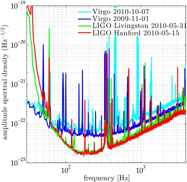
Figure 1. Best strain noise spectra from the LIGO and Virgo detectors during the 2009–2010 science runs.
Download figure:
Standard image High-resolution imageThe GEO 600 detector (Grote et al. 2008), located near Hannover, Germany, was also operational in 2009–2010, though with a lower sensitivity than LIGO and Virgo. We do not use the GEO data in this search as the modest gains in the sensitivity to GW signals would not have offset the increased complexity of the analysis. However, GEO data are used in searches for gravitational waves coincident with GRBs occurring during periods when only one of the LIGO or Virgo detectors is operational, such as the period between the fifth and sixth LIGO science runs and during summer 2011. The result of those searches will be reported in a future publication.
4. GRB SAMPLE
We obtained our sample of GRB triggers from the GRB Coordinates Network118 (GCN; Barthelmy 2008), supplemented by the Swift119 and Fermi120 trigger pages. This sample of GRB triggers came mostly from the Swift satellite (Gehrels et al. 2004) and the Fermi satellite (Meegan et al. 2009), but several triggers also came from other spaceborne experiments, such as MAXI (Matsuoka et al. 2009), SuperAGILE (Feroci et al. 2007), and INTEGRAL (Winkler et al. 2003), as well as from time-of-flight triangulation using satellites in the third InterPlanetary network (IPN; Hurley et al. 2009).
In total there are 404 GRBs in our GRB sample during the 2009–2010 LIGO–Virgo science runs. About 10% of the GRBs have associated redshift measurements, all of them evidently beyond the reach of current GW detectors. Nevertheless, times around these GRBs have been analyzed in case of, for example, a chance association with an incorrect host galaxy.
GRBs that occurred when two or more of the LIGO and Virgo detectors were operating in a resonant and stable configuration are analyzed. Data segments which are flagged as being of poor quality are excluded from the analysis. In total, 154 GRBs were analyzed, out of which 150 GRBs were analyzed by the GW burst search, and 26 short GRBs were analyzed by the coalescence search. (As the GW data-quality requirements are somewhat different for the unmodeled burst and coalescence searches, four short GRBs analyzed by the coalescence search could not be analyzed by the GW burst search.)
The classification of GRBs into short and long is somewhat ambiguous (Gehrels et al. 2006; Bloom et al. 2008; Zhang et al. 2009; Horvath et al. 2010). Since binary mergers are particularly strong sources of gravitational radiation, we make use of a more lenient classification to identify GRBs which may originate from a binary merger (Zhang et al. 2007, 2009). Our selection is based on the T90 duration (the time interval over which 90% of the total background-subtracted photon counts are observed), and on visual inspection of all available light curves. Specifically, we treat as "short" all GRBs with T90 < 4 s; this choice, rather than the standard 2 s cutoff for short GRBs, is to ensure we include those short GRBs in the tail of the duration distribution. In addition, some of the longer-duration GRBs exhibit a prominent short spike at the beginning of the light curve and an extended longer emission (Norris & Bonnell 2006), suggesting that those GRBs might be created by the merger of two compact objects. Those GRBs were also treated as short GRBs and, where necessary, the trigger time used for the coalescence search was shifted by up to a few seconds to match the rising edge of the spike (which should correspond to the binary coalescence time). This lenient classification ensures a relatively complete sample, at the price of sample purity—some of the GRBs we analyze as "short" may not have a compact binary progenitor. This impurity is acceptable for the purpose of GW detection where we do not want to miss a potentially observable GW counterpart. The final set of 26 short GRBs is given in Table 1.
Table 1. Short GRB Sample and Search Results
| GRB Name | UTC | R.A. | Decl. | Network and | Exclusion (Mpc) | NS–NS | NS–BH | γ-Ray Detector | |
|---|---|---|---|---|---|---|---|---|---|
| Time | Time Window | GW Burst at | |||||||
| 150 Hz | 300 Hz | ||||||||
| 090720B‡ | 17:02:56 | 13h31m59s | −54°48' | L1V1 | 7.1 | 3.8 | 8.6 | 16.0 | GBM |
| 090802A | 05:39:03 | 5h37m19s | 34°05' | H1L1V1 | 7.3 | 2.6 | 6.5 | 11.3 | GBM and IPN |
| 090815C | 23:21:39 | 4h17m57s | −65°57' | H1L1V1* | 29.8 | 12.0 | 24.6 | 44.3 | BAT |
| 090820B‡ | 12:13:16 | 21h13m02s | −18°35' | H1V1 | 12.2 | 5.8 | 15.1 | 26.3 | GBM |
| 090831A‡ | 07:36:36 | 9h40m23s | 50°58' | H1V1† | 7.2 | 2.1 | 4.6 | 8.9 | GBM |
| 090927 | 10:07:16 (+1) | 22h55m42s | −70°58' | H1L1V1 | 16.0 | 9.0 | 19.8 | 35.1 | BAT |
| 091018‡ | 20:48:19 | 2h08m46s | −57°33' | H1V1 | ... | ... | 5.2 | 10.0 | BAT |
| 091126A | 07:59:24 | 5h33m00s | −19°16' | H1V1 | ... | ... | 13.9 | 25.3 | GBM |
| 091127‡ | 23:25:45 | 2h26m19s | −18°57' | L1V1* | 5.9 | 2.3 | 3.1 | 4.9 | BAT |
| 091208B‡ | 09:49:57 | 1h57m39s | 16°53' | H1V1 | ... | ... | 11.4 | 20.6 | BAT |
| 100111A‡ | 04:12:49 | 16h28m06s | 15°32' | H1L1 | 18.8 | 8.6 | 17.7 | 30.4 | BAT |
| 100206A | 13:30:05 | 3h08m40s | 13°10' | H1L1 | 21.0 | 8.8 | 19.1 | 34.1 | BAT |
| 100213A | 22:27:48 | 23h17m30s | 43°22' | H1L1 | 22.4 | 10.0 | 24.5 | 46.3 | BAT |
| 100216A | 10:07:00 | 10h17m03s | 35°31' | H1L1 | 29.1 | 13.0 | 22.7 | 40.1 | BAT |
| 100316B | 08:01:36 | 10h54m00s | −45°28' | H1L1 | ... | ... | 2.1 | 3.7 | BAT |
| 100322B | 07:06:18 | 5h05m57s | 42°41' | H1L1 | 18.5 | 7.4 | 14.8 | 25.4 | BAT |
| 100325B‡ | 05:54:43 | 13h56m33s | −79°06' | H1L1 | 21.8 | 8.7 | 19.0 | 34.3 | GBM |
| 100328A | 03:22:44 | 10h23m45s | 47°02' | H1L1 | 28.9 | 12.4 | 30.1 | 51.3 | GBM |
| 100515A‡ | 11:13:09 | 18h21m52s | 27°01' | H1L1 | 38.2 | 17.1 | 37.1 | 64.5 | GBM |
| 100517D‡ | 03:42:08 | 16h14m21s | −10°22' | H1L1 | 3.4 | 2.7 | 7.7 | 12.1 | GBM |
| 100628A | 08:16:40 | 15h03m46s | −31°39' | H1L1 | 20.6 | 8.3 | 20.7 | 36.7 | BAT |
| 100717446♯ | 10:41:47 | 20h17m14s | 19°32' | H1L1 | 31.3 | 13.2 | 26.5 | 46.1 | GBM |
| 100816A | 00:37:51 | 23h26m57s | 26°34' | L1V1 | 9.5 | 5.8 | 6.6 | 11.5 | BAT |
| 100905A | 15:08:14 (−1) | 2h06m10s | 14°55' | H1L1V1◊ | 17.3 | 6.3 | 11.5 | 19.6 | BAT |
| 100924A‡ | 03:58:08 | 0h02m41s | 7°00' | H1L1V1† ◊ | 29.2 | 12.0 | 22.8 | 39.4 | BAT |
| 100928A | 02:19:52 (+1) | 14h52m08s | −28°33' | H1L1V1◊ | 26.1 | 10.1 | 20.1 | 35.1 | BAT |
Notes. Information and limits on associated GW emission for each of the analyzed GRBs that were classified by us as short. The first four columns are: the GRB name in YYMMDD format or the Fermi/GBM trigger ID for GBM triggers classified as a GRB without an available GRB name (see http://heasarc.gsfc.nasa.gov/W3Browse/fermi/fermigbrst.html and Paciesas et al. 2012); the trigger time (numbers in parentheses denote the time in seconds by which the trigger was shifted for the coalescence search following visual inspection of the light curve); and the sky position used for the GW search (right ascension and declination). Both a ♯ and a ‡ indicate that, although the formal duration of this GRB is longer than 4 s (‡), or unavailable (♯), the GRB was analyzed as a short GRB because of a prominent short spike at the beginning of the light curve (see Section 4). The fifth column gives the gravitational wave detector network used; a * indicates when the shorter on-source window starting 120 s before the trigger is used for the GW burst search, and a † when the on-source window is extended to cover the GRB duration (T90 > 60 s). A◊ indicates the use of only H1L1 data for the burst search, because of data-quality requirements. Columns 6–9 display the result of the search: the 90% confidence lower limits on the distance to the GRB for different waveform models. A standard siren energy emission of EGW = 10−2 M☉ c2 is assumed for the circular sine-Gaussian GW burst models; these limits are not available for four short GRBs which were not analyzed by GW burst search. The last column gives the γ-ray detector that provided the sky location used for the search. For GRB 090802, IPN triangulation from Konus-WIND, INTEGRAL, and Fermi was used to further constrain the sky position. The intersection of the IPN and Fermi error regions was used to place search points using the method described in Predoi & Hurley (2012). For this GRB, the quoted right ascension and declination correspond to the center of the Fermi error region. For IPN localizations a complete list of detectors can be found on the project trigger page, http://www.ssl.berkeley.edu/ipn3/masterli.txt.
Download table as: ASCIITypeset image
A large number of GRBs detected by the IPN are not reported by the GCN; the result of a search for GWs associated with those GRBs will be reported in a future publication.
5. SEARCHES FOR GWs ASSOCIATED WITH GRBs
We perform searches for both unmodeled bursts and coalescence signals. We begin this section by describing the basic methodology and features common to both searches, then briefly present the details of the two analysis methods.
5.1. Search Methodology
Both search pipelines identify an "on-source" time in which to search for an associated GW event. This time selection is expected to improve by a factor ∼1.5 the sensitivity of the search compared to an all-sky/all-time search (Kochanek & Piran 1993). For the GW burst search, we use the interval from 600 s before each GRB trigger to either 60 s or the T90 time (whichever is larger) after the trigger as the window in which to search for a GW signal. This conservative window is large enough to take into account most plausible time delays between a GW signal from a progenitor and the onset of the gamma-ray signal, as discussed in Section 2.1. This window is also safely larger than any uncertainty in the definition of the measured GRB trigger time. For cases when less early GW data are available, a shorter window starting 120 s before the GRB trigger time is used. This still covers most time-delay scenarios. For the binary coalescence search, it is believed that the delay between the merger and the emission of γ-rays will be small, as discussed in Section 2.2. We therefore use an interval of 5 s prior to the GRB to 1 s following as the on-source window, which is wide enough to allow for uncertainties in the emission model and in the arrival time of the electromagnetic signal (Abbott et al. 2010a).
The on-source data are scanned by the search algorithms to detect possible GW transients (either coalescence or burst), referred to as "events." For both searches the analysis depends on the sky position of the GRB. GRBs reported by the Swift satellite have very small position uncertainty (≪1°; see Barthelmy et al. 2005), and the GW searches need only be performed at the reported sky location. For GRBs detected by the Gamma-ray Burst Monitor (GBM) on the Fermi satellite (Meegan et al. 2009), however, the sky localization region can be large (≫1°), and detection efficiency would be lost if the GW searches only used a single sky location. To resolve this problem, searches for poorly localized GRBs are done over a grid of sky positions, covering the sky localization region (Wąs 2011; Wąs et al. 2012). We assume a systematic 68% coverage error circle for the Fermi/GBM sky localizations with a radius of 3 2 with 70% probability and a radius of 95 with 30% probability (Connaughton 2011), which is added in quadrature to the reported statistical error.
Each pipeline orders events found in the on-source time according to a ranking statistic. To reduce the effect of non-stationary background noise, candidate events are subjected to checks that "veto" events overlapping in time with known instrumental or environmental disturbances (Aasi et al. 2012). The surviving event with the highest ranking statistic is taken to be the best candidate for a GW signal for that GRB; it is referred to as the loudest event (Brady et al. 2004; Biswas et al. 2009). To estimate the significance of the loudest event, the pipelines also analyze coincident data from a period surrounding the on-source data, where we do not expect a signal. The proximity of these off-source data to the on-source data makes it likely that the estimated background will properly reflect the noise properties in the on-source segment. The off-source data are processed identically to the on-source data; in particular, the same data-quality cuts and consistency tests are applied, and the same sky positions relative to the GW detector network are used. If necessary, to increase the background distribution statistics, multiple time shifts are applied to the data streams from different detector sites, and the off-source data re-analyzed for each time shift.
To determine if a GW is present in the on-source data, the loudest on-source event is compared to the distribution of loudest off-source events. A p-value is defined as the probability of obtaining such an event or louder in the on-source data, given the background distribution, under the null hypothesis. The triggers with the smallest p-values in the searches are subjected to additional follow-up studies to determine if the events can be associated with some non-GW noise artifact, for example due to an environmental disturbance.
Regardless of whether a statistically significant signal is present, we also set a 90% confidence level lower limit on the distance to the GRB progenitor for various signal models. This is done by adding simulated GW signals to the data and repeating the analyses. These signals, which are drawn from astrophysically motivated distributions described in the following sections, are used to calculate the maximum distance for which there is a 90% or greater chance that such a signal model, if present in the on-source region, would have produced an event with larger ranking statistic than the largest value actually measured.
5.2. Search for GW Bursts
The search procedure for GW bursts follows that used in the 2005–2007 GRB search (Abbott et al. 2010b). All GRBs are treated identically, without regard to redshift (if known), fluence, or classification. The on-source data are scanned by the X-Pipeline algorithm (Sutton et al. 2010; Wąs et al. 2012), which is designed to detect short GW bursts, ≲ 1 s, in the 60–500 Hz frequency range. X-Pipeline combines data from arbitrary sets of detectors, taking into account the antenna response and noise level of each detector to improve the search sensitivity. Time–frequency maps of the combined data streams are scanned for clusters of pixels with energy significantly higher than that expected from background noise. The resulting candidate GW events are characterized by a ranking statistic based on energy. We also apply consistency tests based on the signal correlations measured between the detectors, assuming a circularly polarized GW, to reduce the number of background events. (The circular polarization assumption is motivated by the fact that the GRB system rotation axis should be pointing roughly at the observer, as discussed in Section 2.1.) The stringency of these tests is tuned by comparing their effect on background events and simulated signal events. The background samples are constructed using the ±1.5 hr of data around the GRB trigger, excluding the on-source time. Approximately 800 time shifts of these off-source data are used to obtain a large sample of background events.
To obtain signal samples, simulated signals are added to the on-source data. The models of GW emission by extreme stellar collapse described in Section 2.1 do not predict the exact shape of the emitted GW signal. As an ad hoc model, we use the GW emission by a rigidly rotating quadrupolar mass moment with a Gaussian time evolution of its magnitude. For such a source with a rotation axis inclined by an angle ι with respect to the observer the received GW signal is a sine-Gaussian
where the signal frequency f0 is equal to twice the rotation frequency, t is the time relative to the signal peak time, Q characterizes the number of cycles for which the quadrupolar mass moment is large, EGW is the total radiated energy, and r is the distance to the source. We consider two sets121 of such signals with signal frequencies f0 of 150 Hz and 300 Hz, which cover the sensitive frequency band of this GW burst search. The inclination angle is distributed uniformly in cos ι, with ι between 0° and 5°, which corresponds to the typical jet opening angle of ∼5° observed for long GRBs (Gal-Yam 2006; Racusin et al. 2009).
Systematic errors are marginalized over in the sensitivity estimation by "jittering" the simulated signals before adding them to the detector noise. This includes distributing injections across the sky according to the gamma-ray satellites' sky location error box, and jittering the signal amplitude, phase, and timing in each detector according to the given detector calibration errors (Accadia et al. 2011; Bartos et al. 2011). This procedure also ensures that the consistency tests used in the analysis are loose enough to allow for such errors.
5.3. Search for GWs from a Compact Binary Progenitor
The core of the coalescence search involves correlating the measured data against theoretically predicted waveforms using matched filtering (Helmstrom 1968). GWs from the inspiral phase of a coalescence are modeled by post-Newtonian approximants in the band of the detector's sensitivity for a wide range of binary masses (Blanchet 2006). The expected GW signal depends on the masses and spins of the NS and its companion (either NS or BH), as well as the distance to the source, its sky position, its inclination angle, and the polarization angle of the orbital axis. Matched filtering is most sensitive to the phase evolution of the signal, which depends on the binary masses and spins, the time of merger, and a fiducial phase. The time and phase can be determined analytically. Ignoring spin, we can therefore perform matched filtering over a discrete two-dimensional bank of templates which span the space of component masses. This bank is constructed such that the maximum loss in signal-to-noise ratio for a binary with negligible spins is 3% (Cokelaer 2007; Harry & Fairhurst 2011). For this search, as in the 2005–2007 GRB search (Abbott et al. 2010a), we used "TaylorF2" frequency domain templates, generated at 3.5 post-Newtonian order (Blanchet et al. 1995, 2004). While the spin of the components is ignored in the template waveforms, we evaluate the efficiency of the search using simulated signals including spin, as described below.
For each short GRB, the detector data streams are combined coherently and searched using the methods described in detail in Harry & Fairhurst (2011). Various signal consistency tests are then applied to reject non-stationary noise artifacts. These include χ2 tests (Allen 2005; Hanna 2008), a null stream consistency test, and a re-weighting of the signal-to-noise ratio to take into account the values recorded by these tests. This is the first coherent search for coalescence signals; it has been found to be more sensitive to GW signals than the coincidence technique used in previous triggered coalescence searches of LIGO and Virgo data (Harry & Fairhurst 2011). Tests using the simulations described below have also shown that this focused coalescence search is a factor of ∼2 more sensitive to coalescence signals than the unmodeled search described in the previous section, justifying the use of a specialized search for this signal type.
To estimate the efficiency of the search and calculate exclusion distances for short GRBs, we draw simulations from two sets of astrophysically motivated compact binary systems: two neutron stars (NS–NS) and a neutron star with a black hole (NS–BH). The NS masses are chosen from a Gaussian distribution centered at 1.4 M☉ (Kiziltan et al. 2010; Ozel et al. 2012) with a width of 0.2 M☉ for the NS–NS case, and a broader spread of 0.4 M☉ for the NS–BH systems, to account for larger uncertainties given the lack of observations for such systems. The BH masses are Gaussian distributed with a mean of 10 M☉ and a width of 6 M☉. The BH mass is restricted such that the total mass of the system is less than 25 M☉. For masses greater than this, the NS would be "swallowed whole" by the BH, no massive torus would form, and no GRB would be produced (Duez 2010; Ferrari et al. 2010; Shibata & Taniguchi 2011).
Observed pulsar spin periods and assumptions about the spin-down rates of neutron stars place the NS spin periods at birth in the range of 10–140 ms, corresponding to an upper limit on S/m2 of ⩽0.04 (Mandel & O'Shaughnessy 2010), where S denotes the spin of the neutron star and m its mass. However, neutron stars can be spun up to much higher spins (e.g., to 716 Hz; Hessels et al. 2006); hence we conservatively assume a maximum spin of S/m2 < 0.4 corresponding to a ∼1 ms pulsar. Therefore, the spin magnitudes are drawn uniformly from the range [0, 0.4]. For BHs the magnitudes are chosen uniformly in the [0, 0.98) range (Mandel & O'Shaughnessy 2010). The spins are oriented randomly, with a constraint on the tilt angle (the angle between the spin direction of the BH and the orbital angular momentum). Since the merger needs to power a GRB, a sufficiently massive accretion disk around the BH is required. Population synthesis studies indicate that the tilt angle is predominantly below 45° (Belczynski et al. 2008); numerical simulations show that for tilt angles larger than 40° the mass of the disk will drop rapidly (Foucart et al. 2011) and BHs with tilt angle >60° will "swallow" the NS completely, leaving no accretion disk to power a GRB (Rantsiou et al. 2008). In our simulations we use the weakest of these three constraints and set the tilt angle to be <60°.
The outflow from a GRB is most likely to be along the direction of the total angular momentum J of the system as discussed in Section 2.2. Observations suggest that this outflow is confined within a cone, whose half-opening angle is estimated to range between several degrees to over 60° for short GRBs (see, e.g., Burrows et al. 2006; Grupe et al. 2006; Dietz 2011). Under the assumption that this cone is centered along the total angular momentum J of the system, we chose the inclination angle between J and the line of sight to the observer to be distributed within cones of half-opening angles 10°, 30°, 45°, and 90°. The majority of the results quoted in this work assume a 30° angle.
The coalescence time is uniform over the on-source region, and the sky position of the GRB is jittered according to the reported uncertainty of the location.
The quoted exclusion distances are marginalized over systematic errors that are inherent in this analysis. First, there is some uncertainty in how well our post-Newtonian templates will match real GW signals; we expect a loss in signal-to-noise ratio of up to 10% because of this mismatch (Abbott et al. 2009b). Second, there is uncertainty in the amplitude calibration of the detectors (Bartos et al. 2011; Accadia et al. 2011); phase and timing calibration uncertainties are also present, but are negligible compared to other sources of errors.
An opportunistic search for coalescence signals has also been performed on the long GRBs. This search is done to conservatively account for uncertainties in the details of the short/long GRB classification, and for uncertainties in the progenitor model of long GRBs for which an associated SN signature was excluded (Gehrels et al. 2006; Watson et al. 2007; Gao et al. 2010). We use the same analysis to check for a coalescence signal associated with long GRBs, but do not estimate exclusion distances as the compact binary coalescence progenitor model is unlikely for long GRBs.
5.4. Significance of p-value Distribution
In addition to evaluating individual p-values, we use a weighted binomial test to assess whether the obtained set of p-values is compatible with the uniform distribution expected from noise only, for both the GW burst and coalescence searches. This test looks for deviations from the null hypothesis in the 5% tail of lowest p-values weighted by the prior probability of detection (estimated from the GW search sensitivity). The weighted binomial test is an extension of the binomial test that has been used in previous searches for GW bursts associated with GRBs (Abbott et al. 2008b, 2010b). The combination of p-values with prior detection probabilities gives more weight to GRBs for which the GW detectors had better sensitivity and therefore the detection of a GW signal is more likely. The details of this test are given in Appendix A.
The result of the weighted binomial test is a single ranking statistic Sweighted. The statistical significance of the measured Sweighted is assessed by comparing to the background distribution of this statistic from Monte Carlo simulations with p-values uniformly distributed in [0, 1]. This yields the overall background probability of the measured set of p-values.
6. RESULTS
The coalescence analysis has been applied to search for signals in coincidence with 26 short GRBs; the GW burst analysis has been applied to 150 GRBs, which include 22 of the 26 short GRBs analyzed by the coalescence search. (As mentioned in Section 4, four of the short GRBs analyzed by the coalescence search could not be analyzed by the GW burst search.) The lists of analyzed GRBs classified as short and long are given in Tables 1 and 2.
Table 2. Long GRB Sample and Search Results
| GRB Name | UTC | R.A. | Decl. | Network and | Exclusion (Mpc) | γ-Ray Detector | |
|---|---|---|---|---|---|---|---|
| Time | Time Window | GW Burst at | |||||
| 150 Hz | 300 Hz | ||||||
| 090709B | 15:07:42 | 6h14m05s | 64°05' | L1V1 | 12.4 | 6.1 | BAT |
| 090717A | 00:49:32 | 5h47m19s | −64°11' | H1V1*† | 19.9 | 9.7 | GBM |
| 090719 | 01:31:26 | 22h45m04s | −67°52' | H1V1 | 10.6 | 6.3 | GBM |
| 090720A | 06:38:08 | 13h34m46s | −10°20' | L1V1 | 12.5 | 6.4 | BAT |
| 090726B | 05:14:07 | 16h01m48s | 36°45' | H1L1V1 | 20.2 | 6.4 | GBM |
| 090726 | 22:42:27 | 16h34m43s | 72°52' | H1V1† | 17.1 | 9.3 | BAT |
| 090727 | 22:42:18 | 21h03m40s | 64°56' | L1V1† | 10.4 | 4.9 | BAT |
| 090727B | 23:32:29 | 22h53m25s | −46°42' | L1V1 | 3.3 | 1.8 | IPN |
| 090802B | 15:58:23 | 17h48m04s | −71°46' | H1L1V1 | 20.5 | 8.3 | GBM |
| 090807 | 15:00:27 | 18h14m57s | 10°17' | H1V1† | 9.8 | 5.3 | BAT |
| 090809 | 17:31:14 | 21h54m39s | −0°05' | H1L1V1 | 19.2 | 6.4 | BAT |
| 090809B | 23:28:14 | 6h20m60s | 0°10' | L1V1 | 9.5 | 4.9 | GBM |
| 090810A | 15:49:07 | 11h15m43s | −76°24' | H1V1 | 14.6 | 7.1 | GBM |
| 090814A | 00:52:19 | 15h58m27s | 25°35' | L1V1† | 9.9 | 6.1 | BAT |
| 090814B | 01:21:01 | 4h19m05s | 60°35' | L1V1 | 10.9 | 5.6 | IBIS |
| 090814D | 22:47:28 | 20h30m35s | 45°43' | H1L1V1 | 17.2 | 6.3 | GBM |
| 090815A | 07:12:12 | 2h44m07s | −2°44' | H1L1V1† | 5.4 | 1.3 | GBM |
| 090815B | 10:30:41 | 1h25m40s | 53°26' | H1V1 | 10.6 | 5.6 | GBM |
| 090815D | 22:41:46 | 16h45m02s | 52°56' | L1V1 | 15.7 | 6.9 | GBM |
| 090823B | 03:10:53 | 3h18m07s | −17°35' | L1V1 | 5.9 | 2.7 | GBM |
| 090824A | 22:02:19 | 3h06m35s | 59°49' | H1V1 | 9.4 | 4.8 | GBM |
| 090826 | 01:37:31 | 9h22m28s | −0°07' | H1V1 | 2.7 | 0.4 | GBM |
| 090827 | 19:06:26 | 1h13m44s | −50°54' | H1V1 | 15.1 | 8.6 | BAT |
| 090829B | 16:50:40 | 23h39m57s | −9°22' | H1V1† | 9.0 | 4.8 | GBM |
| 090926B | 21:55:48 | 3h05m14s | −38°60' | H1L1V1† | 19.1 | 7.5 | BAT |
| 090929A | 04:33:03 | 3h26m47s | −7°20' | H1V1 | 8.7 | 4.4 | GBM |
| 091003 | 04:35:45 | 16h45m33s | 36°35' | L1V1 | 8.8 | 3.2 | LAT |
| 091017A | 20:40:24 | 14h03m11s | 25°29' | H1V1 | 7.5 | 4.9 | GBM |
| 091018B | 22:58:20 | 21h27m19s | −23°05' | L1V1 | 3.6 | 1.6 | GBM |
| 091019A | 18:00:40 | 15h04m07s | 80°20' | H1L1V1 | 20.4 | 8.2 | GBM |
| 091020 | 21:36:44 | 11h42m54s | 50°59' | L1V1 | 9.5 | 5.2 | BAT |
| 091026B | 11:38:48 | 9h08m19s | −23°39' | H1V1 | 5.1 | 3.0 | GBM |
| 091030A | 19:52:26 | 2h46m40s | 21°32' | H1V1† | 11.5 | 4.9 | GBM |
| 091031 | 12:00:28 | 4h46m47s | −57°30' | H1V1† | 14.2 | 6.2 | LAT |
| 091103A | 21:53:51 | 11h22m24s | 11°18' | L1V1 | 5.1 | 2.2 | GBM |
| 091109A | 04:57:43 | 20h37m00s | −44°11' | H1V1 | 13.0 | 7.3 | BAT |
| 091109B | 21:49:03 | 7h31m00s | −54°06' | H1V1 | 14.2 | 8.7 | BAT |
| 091115A | 04:14:50 | 20h31m02s | 71°28' | H1L1V1* | 14.1 | 7.2 | GBM |
| 091122A | 03:54:20 | 7h23m26s | 0°34' | H1V1 | 11.9 | 5.5 | GBM |
| 091123B | 01:55:59 | 22h31m16s | 13°21' | L1V1* | 9.8 | 5.4 | GBM |
| 091128 | 06:50:34 | 8h30m45s | 1°44' | H1V1 | 6.7 | 3.1 | GBM |
| 091202B | 01:44:06 | 17h09m59s | −1°54' | H1V1 | 10.5 | 4.6 | GBM |
| 091202C | 05:15:42 | 0h55m26s | 9°05' | H1V1 | 12.6 | 6.2 | GBM |
| 091202 | 23:10:04 | 9h15m18s | 62°33' | H1V1 | 14.4 | 6.5 | IBIS |
| 091215A | 05:37:26 | 18h52m59s | 17°33' | H1L1* | 18.5 | 8.1 | GBM |
| 091219A | 11:04:45 | 19h37m57s | 71°55' | H1L1V1 | 12.4 | 6.1 | GBM |
| 091220A | 10:36:50 | 11h07m04s | 4°49' | H1L1V1 | 21.0 | 8.6 | GBM |
| 091223B | 12:15:53 | 15h25m04s | 54°44' | H1L1 | 24.3 | 9.9 | GBM |
| 091224A | 08:57:36 | 22h04m40s | 18°16' | H1L1 | 16.4 | 6.4 | GBM |
| 091227A | 07:03:13 | 19h47m45s | 2°36' | H1L1V1 | 19.7 | 8.6 | GBM |
| 100101A | 00:39:49 | 20h29m16s | −27°00' | H1L1* | 9.1 | 4.5 | GBM |
| 100103A | 17:42:32 | 7h29m28s | −34°29' | H1L1V1 | 26.0 | 12.1 | IBIS |
| 100112A | 10:01:17 | 16h00m33s | −75°06' | H1L1 | 15.7 | 7.5 | GBM |
| 100201A | 14:06:17 | 8h52m24s | −37°17' | H1L1* | 25.9 | 10.8 | GBM |
| 100212B | 13:11:45 | 8h57m04s | 32°13' | H1L1* | 6.8 | 3.7 | GBM |
| 100213B | 22:58:34 | 8h17m16s | 43°28' | H1L1 | 15.6 | 7.1 | BAT |
| 100219A | 15:15:46 | 10h16m48s | −12°33' | H1L1 | 17.3 | 6.7 | BAT |
| 100221A | 08:50:26 | 1h48m28s | −17°25' | H1L1 | 29.1 | 12.5 | GBM |
| 100225B | 05:59:05 | 23h31m24s | 15°02' | H1L1 | 20.0 | 8.3 | GBM |
| 100225C | 13:55:31 | 20h57m04s | 0°13' | H1L1* | 13.7 | 5.8 | GBM |
| 100228B | 20:57:47 | 7h51m57s | 18°38' | H1L1 | 13.8 | 6.8 | GBM |
| 100301B | 05:21:46 | 13h27m24s | 19°50' | H1L1 | 24.0 | 9.1 | GBM |
| 100315A | 08:39:12 | 13h55m35s | 30°08' | H1L1 | 43.5 | 16.9 | GBM |
| 100316A | 02:23:00 | 16h47m48s | 71°49' | H1L1 | 18.2 | 6.9 | BAT |
| 100316C | 08:57:59 | 2h09m14s | −67°60' | H1L1 | 39.4 | 16.5 | BAT |
| 100324A | 00:21:27 | 6h34m26s | −9°44' | H1L1 | 34.3 | 12.6 | BAT |
| 100324B | 04:07:36 | 2h38m41s | −19°17' | H1L1 | 20.2 | 7.3 | IPN |
| 100325A | 06:36:08 | 22h00m57s | −26°28' | H1L1 | 36.7 | 14.1 | LAT |
| 100326A | 07:03:05 | 8h44m57s | −28°11' | H1L1 | 13.1 | 5.6 | GBM |
| 100331B | 21:08:38 | 20h11m56s | −11°04' | H1L1 | 14.1 | 6.1 | AGILE |
| 100401A | 07:07:31 | 19h23m15s | −8°15' | H1L1† | 17.6 | 6.2 | BAT |
| 100410A | 08:31:57 | 8h40m04s | 21°29' | H1L1* | 3.6 | 1.5 | GBM |
| 100410B | 17:45:46 | 21h16m59s | 37°26' | H1L1 | 28.3 | 12.7 | GBM |
| 100418A | 21:10:08 | 17h05m25s | 11°27' | H1L1 | 26.5 | 11.8 | BAT |
| 100420B | 00:12:06 | 8h02m11s | −5°49' | H1L1 | 32.6 | 12.5 | GBM |
| 100420A | 05:22:42 | 19h44m21s | 55°45' | H1L1 | 19.1 | 7.5 | BAT |
| 100423B | 05:51:25 | 7h58m40s | 5°47' | H1L1 | 18.6 | 6.4 | GBM |
| 100425A | 02:50:45 | 19h56m38s | −26°28' | H1L1 | 41.4 | 15.6 | BAT |
| 100427A | 08:31:55 | 5h56m41s | −3°28' | H1L1 | 25.5 | 11.2 | BAT |
| 100502A | 08:33:02 | 8h44m02s | 18°23' | H1L1 | 4.0 | 2.6 | GBM |
| 100507A | 13:51:15 | 0h11m36s | −79°01' | H1L1 | 23.9 | 7.8 | GBM |
| 100508A | 09:20:42 | 5h05m03s | −20°45' | H1L1* | 47.3 | 18.2 | BAT |
| 100516A | 08:50:41 | 18h17m38s | −8°12' | H1L1 | 28.9 | 11.1 | GBM |
| 100516B | 09:30:38 | 19h50m43s | 18°40' | H1L1 | 35.0 | 14.3 | GBM |
| 100517B | 01:43:08 | 6h43m43s | −28°59' | H1L1 | 18.6 | 7.0 | GBM |
| 100517E | 05:49:52 | 0h41m45s | 4°26' | H1L1 | 26.8 | 10.5 | GBM |
| 100517F | 15:19:58 | 3h30m55s | −71°52' | H1L1 | 23.9 | 10.2 | GBM |
| 100517C | 03:09:50 | 2h42m31s | −44°19' | H1L1 | 35.9 | 13.6 | GBM |
| 100526B | 19:00:38 | 0h03m06s | −37°55' | H1L1† | 12.5 | 5.4 | BAT |
| 100604A | 06:53:34 | 16h33m12s | −73°11' | H1L1 | 19.3 | 9.0 | GBM |
| 100608A | 09:10:06 | 2h02m09s | 20°27' | H1L1 | 24.9 | 10.4 | GBM |
| 100701B | 11:45:23 | 2h52m26s | −2°13' | H1L1 | 14.1 | 6.3 | GBM |
| 100709A | 14:27:32 | 9h30m07s | 17°23' | H1L1 | 16.9 | 6.5 | GBM |
| 100717372 | 08:55:06 | 19h08m14s | −0°40' | H1L1 | 27.3 | 10.7 | GBM |
| 100719989 | 23:44:04 | 7h33m12s | 5°24' | H1L1 | 15.3 | 5.9 | GBM |
| 100722291 | 06:58:24 | 2h07m14s | 56°14' | H1L1* | 17.7 | 6.7 | GBM |
| 100725A | 07:12:52 | 11h05m52s | −26°40' | H1L1† | 35.5 | 14.0 | BAT |
| 100725B | 11:24:34 | 19h20m06s | 76°57' | H1L1† | 25.9 | 10.8 | BAT |
| 100727A | 05:42:17 | 10h16m44s | −21°25' | H1L1† | 31.3 | 12.6 | BAT |
| 100802A | 05:45:36 | 0h09m55s | 47°45' | H1L1† | 36.4 | 16.3 | BAT |
| 100804104 | 02:29:26 | 16h35m52s | 27°27' | H1L1 | 40.4 | 18.0 | GBM |
| 100814A | 03:50:11 | 1h29m54s | −17°59' | H1L1V1† | 17.3 | 7.3 | BAT |
| 100814351 | 08:25:25 | 8h11m16s | 18°29' | L1V1* | 14.1 | 8.0 | GBM |
| 100816009 | 00:12:41 | 6h48m28s | −26°40' | L1V1* | 6.6 | 3.5 | GBM |
| 100819498 | 11:56:35 | 18h38m23s | −50°02' | H1L1V1 | 30.1 | 12.5 | GBM |
| 100820373 | 08:56:58 | 17h15m09s | −18°31' | H1L1V1 | 18.2 | 7.2 | GBM |
| 100823A | 17:25:35 | 1h22m49s | 5°51' | H1L1V1* | 8.7 | 4.0 | BAT |
| 100825287 | 06:53:48 | 16h53m45s | −56°34' | H1L1V1 | 18.7 | 7.3 | GBM |
| 100826A | 22:58:22 | 19h05m43s | −32°38' | L1V1 | 4.8 | 2.3 | GBM |
| 100829876 | 21:02:08 | 6h06m52s | 29°43' | H1L1V1 | 12.3 | 4.7 | GBM |
| 100904A | 01:33:43 | 11h31m37s | −16°11' | L1V1 | 13.1 | 7.3 | BAT |
| 100905907 | 21:46:22 | 17h30m36s | 13°05' | H1L1V1 | 17.8 | 7.5 | GBM |
| 100906A | 13:49:27 | 1h54m47s | 55°38' | H1L1*† | 30.5 | 12.2 | BAT |
| 100916A | 18:41:12 | 10h07m50s | −59°23' | H1L1V1 | 8.3 | 3.6 | GBM |
| 100917A | 05:03:25 | 19h16m59s | −17°07' | H1L1V1† | 18.2 | 8.0 | BAT |
| 100918863 | 20:42:18 | 20h33m38s | −45°58' | H1L1V1 | 19.4 | 7.8 | GBM |
| 100919884 | 21:12:16 | 10h52m57s | 6°01' | H1L1V1 | 19.9 | 10.3 | GBM |
| 100922625 | 14:59:43 | 23h47m55s | −25°11' | H1V1 | 9.2 | 4.7 | GBM |
| 100926595 | 14:17:03 | 14h50m59s | −72°21' | H1L1 | 29.5 | 13.1 | GBM |
| 100926694 | 16:39:54 | 2h54m19s | −11°06' | H1L1V1 | 12.2 | 5.1 | GBM |
| 100929916 | 21:59:45 | 12h12m07s | −24°56' | H1V1 | 10.1 | 6.0 | GBM |
| 101002279 | 06:41:26 | 21h33m23s | −27°28' | H1V1 | 9.5 | 4.6 | GBM |
| 101003244 | 05:51:08 | 11h43m24s | 2°29' | H1L1V1 | 34.1 | 13.1 | GBM |
| 101004426 | 10:13:49 | 15h28m52s | −43°59' | H1L1 | 46.8 | 17.5 | GBM |
| 101010190 | 04:33:46 | 3h08m45s | 43°34' | L1V1 | 9.0 | 4.7 | GBM |
| 101013412 | 09:52:42 | 19h28m19s | −49°38' | H1L1V1 | 35.8 | 15.0 | GBM |
| 101015558 | 13:24:02 | 4h52m38s | 15°28' | H1L1 | 29.9 | 12.4 | GBM |
| 101016243 | 05:50:16 | 8h52m09s | −4°37' | L1V1 | 9.4 | 4.7 | GBM |
Notes. Information and limits on associated GW emission for each of the analyzed GRBs that were classified as long. The first four columns are: the GRB name in YYMMDD format or the Fermi/GBM trigger ID for GBM triggers classified as a GRB without an available GRB name (see http://heasarc.gsfc.nasa.gov/W3Browse/fermi/fermigbrst.html and Paciesas et al. 2012); the trigger time; and the sky position used for the GW search (right ascension and declination). The fifth column gives the gravitational wave detector network used; a * indicates when the shorter on-source window starting 120 s before the trigger is used, and a † when the on-source window is extended to cover the GRB duration (T90 > 60 s). Columns 6–7 display the result of the search: the 90% confidence lower limits on the distance to the GRB for the circular sine-Gaussian GW burst models at 150 Hz and 300 Hz. A standard siren energy emission of EGW = 10−2 M☉ c2 is assumed. The last column gives the γ-ray detector that provided the sky location used for the search. For IPN localizations a complete list of detectors can be found on the project trigger page, http://www.ssl.berkeley.edu/ipn3/masterli.txt.
6.1. GW Burst Search Results
The distribution of p-values for each of the 150 GRBs analyzed by the GW burst search is shown in Figure 2. The weighted binomial test yields a background probability of 25%. Therefore, the distribution is consistent with no GW events being present.
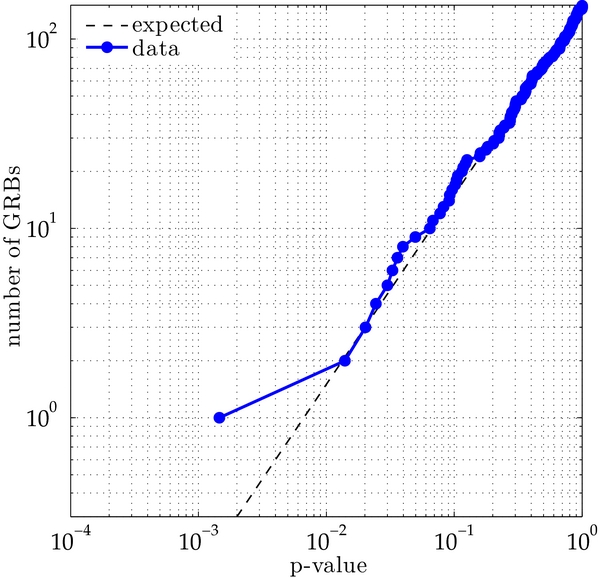
Figure 2. Cumulative p-value distribution from the analysis of 150 GRBs with the GW burst search. The expected distribution under the null hypothesis is indicated by the dashed line.
Download figure:
Standard image High-resolution imageThe smallest p-value, 0.15%, has been obtained for GRB 100917A. This GRB was localized on the sky by Swift; however no redshift measurement is available to date. The corresponding GW event was obtained by combining data from the H1, L1, and V1 detectors. A study of the environmental and instrumental channels at that time yields potential instrumental causes for this event, but is not conclusive. Regardless, the measured p-value is not significant as determined by the weighted binomial test, so this event is not a candidate for a GW detection.
6.2. Coalescence Search Results
The distribution of p-values for each of the 26 short GRBs analyzed by the coalescence search is shown in Figure 3. The result of the weighted binomial test yields a background probability of 8%, corresponding to a 1.8σ deviation from the null hypothesis. However, as we mentioned in Section 4, we use a lenient classification when deciding if GRBs are treated as short or long for the purposes of our analyses. If restrict our short GRB sample to the more commonly used criterion, T90 < 2 s, then we find a background probability of 3%, corresponding to a 2.2σ deviation.

Figure 3. Cumulative p-value distribution from the analysis of 26 short GRBs with the coalescence search. For GRBs where no event is observed in the on-source region, we can only place a lower bound on the p-value; thus we show two distributions where the upper (blue solid line) and lower (green dashed line) bound, respectively, was taken for every GRB. The expected distribution under the null hypothesis is indicated by the dashed line.
Download figure:
Standard image High-resolution imageThis deviation was due to an event found in coincidence with GRB 100328A, which produced the smallest p-value of 1%, and was the GRB to which the search had the second best sensitivity. A follow-up investigation of this candidate determined that it was due to a noise artifact in the Hanford instrument, which was one of a class of glitches caused by a bad power supply which contaminated the length and angular control servos. No other noteworthy events were found by this search and thus there are no potential GW candidates. The opportunistic search for coalescence signals associated with long GRBs did not yield any candidate that was inconsistent with background noise.
7. ASTROPHYSICAL INTERPRETATION
Given that no significant event was found in our analyses, we place limits on GW emission based on the signal models discussed in Section 2, and assess the potential of a similar search with second-generation GW detectors.
7.1. Distance Exclusion
For each GRB we derive a 90% confidence lower limit on the GRB progenitor distance for various emission models using the methodology described in Section 5.1.
The GW burst search provides lower limits on the generic GW burst signal emitted by a rotator described in Section 5.2 for each GRB. We assume that the source emitted EGW = 10−2 M☉ c2 of energy in GWs,122 that the jet opening angle is 5°, and consider emission frequencies of 150 Hz and 300 Hz. The distance limits are given in Tables 1 and 2, and their histogram is shown in Figure 4. The median exclusion distance is D ∼ 17 Mpc (EGW/10−2 M☉ c2)1/2 for emission at frequencies around 150 Hz, where the LIGO–Virgo detector network is most sensitive.

Figure 4. Histograms across the sample of GRBs of the distance exclusions at the 90% confidence level for circularly polarized sine-Gaussian GW burst models at 150 Hz and 300 Hz. We assume an optimistic standard siren GW emission of EGW = 10−2 M☉ c2. See Tables 1 and 2 for the exclusion values for each GRB.
Download figure:
Standard image High-resolution imageThe coalescence search sets lower limits on both the NS–NS and NS–BH models described in Section 5.3 for each short GRB, assuming a jet half-opening angle of 30°. The distance limits are given in Table 1 and a histogram of their values is shown in Figure 5. The median exclusion distance for NS–NS (NS–BH) coalescences is 16 Mpc (28 Mpc) for the 30° cone. We note that these exclusion distances are affected by the choice of signal parameter priors in Section 5.3; for example, Figure 6 shows the median exclusion distances for half-opening angles of 10°, 30°, 45°, and 90°. Since the amplitude of a GW signal is stronger for a face-on binary, the exclusion distance improves for smaller half-opening angles. With no restriction on the opening angle, the 90% exclusion distance decreases significantly, as there are orientations which will give very little observable GW signal in the detector network.
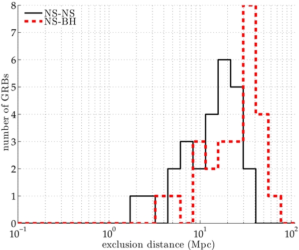
Figure 5. Histograms across the sample of short GRBs of the distance exclusions at the 90% confidence level for NS–NS and NS–BH systems. See Table 1 for the exclusion values for each short GRB.
Download figure:
Standard image High-resolution image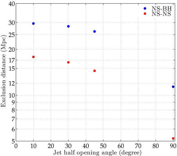
Figure 6. Median exclusion distances of compact binary coalescence sources as a function of half-opening angle, sampled at 10°, 30°, 45°, and 90°. The medians are computed over the set of 26 short GRBs, for both NS–NS and NS–BH, at 90% confidence level.
Download figure:
Standard image High-resolution imageThe GW burst and compact binary coalescence exclusion distances may be compared to those from all-sky searches, which look for GWs without requiring association with a GRB or other external trigger. Figure 7 of Abadie et al. (2012a) presents 50%-confidence exclusion energies for the all-sky GW burst search on this same data set for an assumed source distance of 10 kpc, with a best limit of approximately EGW = 2 × 10⁻⁸ M☉ c2 at 150 Hz. Rescaling to our nominal value of 10−2 M☉ c2 gives an exclusion distance of ∼7 Mpc. Wąs (2011) performs a more rigorous comparison that accounts for the fraction of events that do not produce GRB triggers due to the γ-ray beaming. This indicates that for emission opening angles in the 5°–30° range, the GRB triggered search should detect a similar number of GW events coming from GRB progenitors as that detected by the all-sky search—between 0.1 and 6 times the number detected by the all-sky search. Furthermore, most of the GW events found by the GRB triggered search will be new detections not found by the all-sky search, illustrating the value of GRB satellites for GW detection.
The NS–NS/NS–BH models used for compact binary coalescence exclusions stand on much firmer theoretical ground than the model used for GW burst exclusions. The amplitude of a coalescence signal is well known and depends on the masses and spins of the compact objects whereas the GW burst energy emitted during a GRB is largely unknown and could be orders of magnitude smaller than the chosen nominal value of EGW = 10−2 M☉ c2. In the pessimistic scenario that GRB progenitors have a comparable GW emission to core-collapse supernovae, the emitted energy could be as low as EGW ∼ 10−8 M☉ c2. Such a signal would only be observable with current GW detectors from a galactic source.
7.2. Population Exclusion
As well as a per-GRB distance exclusion, we set an exclusion on GRB population parameters by combining results from the set of analyzed GRBs. To do this, we use a simple population model, where all GRB progenitors have the same GW emission (standard sirens), and perform exclusion on cumulative distance distributions. We parameterize the distance distribution with two components: a fraction F of GRBs distributed with a constant comoving density rate123 up to a luminosity distance R, and a fraction 1 − F at effectively infinite distance. This simple model yields a parameterization of astrophysical GRB distance distribution models that predict a uniform local rate density and a more complex dependence at redshift >0.1, as the large-redshift part of the distribution is well beyond the sensitivity of current GW detectors. The exclusion is then performed in the (F, R) plane. Full details of the exclusion method are given in Appendix B.
The exclusion for GW bursts at 150 Hz with EGW = 10−2 M☉ c2 is shown in Figure 7, whereas the exclusion for the coalescence model for short GRBs is shown in Figure 8. Both exclusions are shown in terms of redshift, where we assume a flat ΛCDM cosmology with Hubble constant H0 = 70 km s−1 Mpc−1, dark matter content ΩM = 0.27, and dark energy content ΩΛ = 0.73 (Komatsu et al. 2011). The exclusion at low redshift is dictated by the number of GRBs analyzed and at high redshift by the typical sensitive range of the search. These exclusions assume 100% purity of the GRB sample. For purity p the cumulative distribution should be rescaled by 1/p; for instance, only one-third of our short GRB sample has a T90 < 2 s. For comparison, each figure also shows the distribution of measured GRB redshifts, for all Swift GRBs (Figure 7) or for all short GRBs (Figure 8). While the distribution of GRBs with measured redshifts includes various observational biases compared to the distribution of all GRBs detected electromagnetically (and on which we perform exclusions), it is clear that the exclusions from the current coalescence and GW burst searches are not sufficient to put any additional constraint on the nature of GRBs.
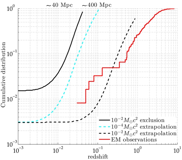
Figure 7. Cumulative redshift distribution F(R) exclusion from the analysis of 150 GRBs with the GW burst search. We exclude at 90% confidence level cumulative distance distributions which pass through the region above the black solid curve. We assume a standard siren sine-Gaussian GW burst at 150 Hz with an energy of EGW = 10−2 M☉ c2. We extrapolate this exclusion to Advanced LIGO/Virgo assuming a factor 10 improvement in sensitivity and a factor 5 increase in the number of GRB triggers analyzed. The black dashed curve is the extrapolation assuming the same standard siren energy of EGW = 10−2 M☉ c2 and the cyan (gray) dashed curve assumes a less optimistic standard siren energy of EGW = 10−4 M☉ c2 (Ott et al. 2006; Romero et al. 2010). For reference, the red staircase curve shows the cumulative distribution of measured redshifts for Swift GRBs (Jakobsson et al. 2006, 2012).
Download figure:
Standard image High-resolution image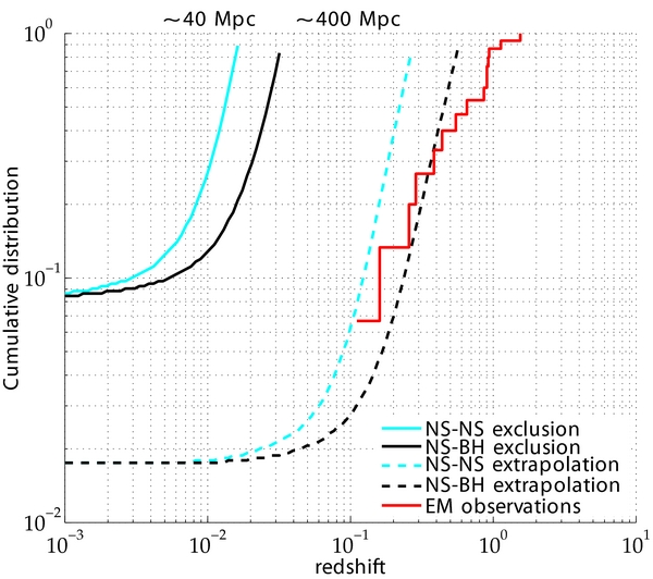
Figure 8. Cumulative redshift distribution F(R) exclusion from the analysis of 26 short GRBs with the coalescence search. Assuming that all the analyzed short GRBs are NS–BH mergers (NS–NS mergers), we exclude at 90% confidence level cumulative distance distributions which pass through the region above the black solid curve (cyan solid curve). The dashed curves are the extrapolation of the solid curves to Advanced LIGO/Virgo, assuming a factor 10 improvement in sensitivity and a factor 5 increase in the number of GRB triggers analyzed. For reference, the red staircase curve shows the cumulative distribution of measured redshifts for short GRBs (Dietz 2011).
Download figure:
Standard image High-resolution imageWhile this search for GW signals in coincidence with observed GRBs was not at the sensitivity necessary to detect such coincidences, it is interesting to consider the chances of detection with the Advanced LIGO/Virgo detectors (Acernese et al. 2009; Harry et al. 2010), which should become operational in 2015. At their design sensitivity, these detectors should offer a factor of 10 improvement in distance sensitivity to both GW burst and coalescence signals, dramatically improving the chances to make a GW observation of an electromagnetically detected GRB.
In Figures 7 and 8 we extrapolate the current exclusion curves to the advanced detector era by assuming a factor 10 increase in sensitivity of the GW detectors and a factor 5 increase in the number of GRBs analyzed (equivalent to approximately 2.5 years of live observing time at the rate that GRBs are currently being reported). These extrapolations show that detection is quite possible in the advanced detector era. Even if a detection is not made, targeted GW searches will allow us to place astrophysically relevant constraints on GRB population models.
For long GRBs, the Advanced LIGO/Virgo detectors will be able to test optimistic scenarios for GW emission—those that produce ∼10−2 M☉ c2 in the most sensitive frequency band of the detectors. The sensitive range for these systems will include the local population of sub-luminous GRBs that produce the low-redshift excess in Figure 7. We note, however, that GW burst emission with significantly lower EGW or at non-optimal frequencies is unlikely to be detectable.
For short GRBs, a coincident GW detection appears quite possible. This conclusion is consistent with simple estimates such as that of Metzger & Berger (2012), who estimate a coincident observation rate of 3 yr−1 (0.3 yr−1) for NS–BH systems (NS–NS systems) with the advanced detectors. The precise rate of occurrence will depend on the typical masses of the compact objects; we are sensitive to NS–BH systems at a larger distance than NS–NS systems. The distribution of binary component spins and the jet opening angle will also affect the received GW signal strength. The detection rate will also depend on the shape of the short GRB cumulative distance curve at low redshift. One must also remember that we used a very optimistic definition of short GRBs to avoid missing a potential signal. It is likely that some of the short GRBs that we analyzed for coalescence signals were not produced by a compact binary progenitor. Even in the case that no coalescence signals are detected in coincidence with short GRBs in the advanced detector era, it should be possible to place astrophysically interesting constraints on the physical characteristics of progenitors of short GRBs.
Finally, we note that these extrapolations carry a number of other uncertainties. In particular, the actual performance of future detectors is unknown. Furthermore, the extrapolations depend on how well the sky will be covered by gamma-ray satellites in 2015 and later compared to the present day.
8. CONCLUSION
We performed searches for GWs coincident with GRBs during the 2009–2010 science runs of LIGO and Virgo. In total we analyzed 154 GRBs using two different analysis methods. A GW burst search looked for unmodeled transient signals, as expected from massive stellar collapses, and a focused search looked for coalescence signals from the merger of two compact objects, as expected for short GRBs. We did not detect any GW in coincidence with a GRB in either search. We set lower limits on the distance of each GRB with the GW burst search, and of the short GRBs with the coalescence search. The median exclusion distances are 17 Mpc (EGW/10−2 M☉ c2)1/2 at 150 Hz for the GW burst search and 16 Mpc (28 Mpc) for NS–NS (NS–BH) systems for the coalescence search, given the priors on the source parameters described in Section 5.
These two searches are more sensitive than the corresponding all-sky searches of the same data (Abadie et al. 2012a, 2012c), due to the more focused analysis possible given the trigger time and sky position information provided by the GRB satellites. This improvement is as much as a factor of ∼2 in distance for the GW burst search. Additionally, our exclusion distances are greater because each source can be presumed to be favorably oriented relative to our line of sight, with limits on misalignment set by inferences of short and long GRB jet opening angles. Further theoretical studies of GRB central engines and observational constraints on jet breaks and jet opening angles could allow this and future studies to refine their constraints a posteriori. Additionally, improved methods of classification of GRBs, and in particular of identifying GRBs with possible binary progenitors with a lower false assignment rate, will improve the performance of our population estimates.
The LIGO and Virgo detectors are currently undergoing a major upgrade, implementing new techniques to greatly increase their sensitivity, and are expected to begin operations by 2015. With these advanced detectors our chances to make a coincident GW observation of a GRB are good, but depend strongly on the advanced detectors running an extended science run at design sensitivity and the number of GRBs that will be observed electromagnetically. Therefore, it is of utmost importance to have GRB satellites operating during the advanced detector era to provide electromagnetic triggers around which a more sensitive search for GWs can be performed.
We are indebted to the observers of the electromagnetic events and the Gamma-ray burst Coordinates Network for providing us with valuable data. The authors gratefully acknowledge the support of the United States National Science Foundation for the construction and operation of the LIGO Laboratory, the Science and Technology Facilities Council of the United Kingdom, the Max-Planck-Society, and the State of Niedersachsen/Germany for support of the construction and operation of the GEO600 detector, and the Italian Istituto Nazionale di Fisica Nucleare and the French Centre National de la Recherche Scientifique for the construction and operation of the Virgo detector. The authors also gratefully acknowledge the support of the research by these agencies and by the Australian Research Council, the International Science Linkages program of the Commonwealth of Australia, the Council of Scientific and Industrial Research of India, the Istituto Nazionale di Fisica Nucleare of Italy, the Spanish Ministerio de Economía y Competitividad, the Conselleria d'Economia Hisenda i Innovació of the Govern de les Illes Balears, the Foundation for Fundamental Research on Matter supported by the Netherlands Organisation for Scientific Research, the Polish Ministry of Science and Higher Education, the FOCUS Programme of Foundation for Polish Science, the Royal Society, the Scottish Funding Council, the Scottish Universities Physics Alliance, the National Aeronautics and Space Administration, the Carnegie Trust, the Leverhulme Trust, the David and Lucile Packard Foundation, the Research Corporation, and the Alfred P. Sloan Foundation. This document has been assigned LIGO Laboratory document number LIGO-P1000121-v10.
APPENDIX A: WEIGHTED BINOMIAL TEST
In a search for GWs associated with GRBs, data corresponding to each GRB are analyzed independently. The results of these independent analyses need to be combined into a single GW (non-)detection statement, which accounts for both the possibility of a single loud GW event or a population of weak GW signals. This weighted binomial test is an extension of the binomial test used to look for an excess of weak GW signatures in previous searches for GW bursts associated with GRBs (Abbott et al. 2008b, 2010b).
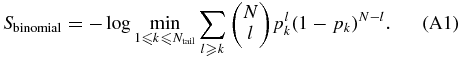
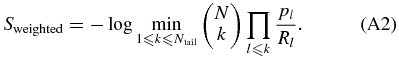
The binomial test considers the set  of p-values obtained for a population of NGRB analyzed GRBs, sorted increasingly. The smallest Ntail = 0.05 NGRB of these p-values are used to search for an excess of weak signals. The binomial probability, under the null hypothesis, of obtaining at least k events with p-values less than the actual kth p-value pk is calculated for 1 ⩽ k ⩽ Ntail and the minimum of these probabilities is used as a detection statistic:
Sbinomial looks for a deviation of the p-value distribution when compared to the uniform distribution expected from background, in the low p-value region where an excess of weak GW signals might be observable. However, this detection statistic does not take into account the relative a priori GW detection probabilities—that is, the sensitive volumes of the GW search associated with each GRB trigger, which depend on the GRB sky position and the performance of GW detectors at that time. To reduce the contribution of GRBs for which the GW detector sensitivity is poor we construct a weighted binomial test (Wąs 2011) as follows.
- 1.Based on the background and sensitivity to simulated signals, compute the distance dk(i) at which the detection efficiency is equal to 50% for GRB k and signal emission model i.
- 2.Compute the relative volume ratio Rk(i) = dk(i)3/max ldl(i)3 for model i compared to the most sensitive GRB.
- 3.Average the relative volume ratio over the different models Rk = meaniRk(i).
- 4.Sort the penalized p-values pk/Rk in increasing order, and compute the detection statistic:

For the GW burst search we use the two coalescence models and three GW burst models given in Sections 5.2 and 5.3 to construct the weighted binomial test, in order to include a range of possible emission models. For the coalescence search we use only the two coalescence models, which is appropriate for that more focused modeled search.
APPENDIX B: POPULATION EXCLUSION METHOD
A lack of detection can be interpreted individually for each analyzed GRB with an exclusion distance for given GW emission models. But the set of analyzed GRBs can also be considered as a whole to derive constraints on the population of GRBs detected by γ-ray satellites. To perform such an exclusion we use a simple population model with all GRB progenitors having the same GW emission (standard sirens), and with a distance distribution with two components: a fraction F of GRBs distributed with a constant comoving rate density up to a luminosity distance R and a fraction 1 − F at effectively infinite distance. This simple model yields a parameterization of astrophysical GRB distance distribution models that predict a uniform local rate density and a more complex dependence at redshift >0.1, as the large-redshift part of the distribution is well beyond the sensitivity of current GW detectors.
For this population model we set a frequentist limit on the F and R parameters by excluding all (F, R) which have a 90% or greater chance of yielding an event with ranking statistic greater than the largest value actually measured for any of the analyzed GRBs. In our computations we assume a flat ΛCDM cosmology with Hubble constant H0 = 70 km s−1 Mpc−1, dark matter content ΩM = 0.27, and dark energy content ΩΛ = 0.73 (Komatsu et al. 2011).
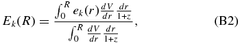
In practice, for each GRB k we measure the efficiency ek(r) as a function of luminosity distance r for a given GW source model of yielding an event with ranking statistic greater than the largest value actually measured. This efficiency is integrated over the volume of radius R, where the sources are distributed with constant rate density. Using the volume element for a flat cosmology,
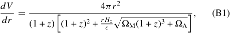
we integrate the efficiency as a function of luminosity distance over the considered volume:
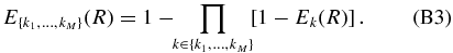
where the additional 1/(1 + z) factor accounts for the redshift of the rate. This volume efficiency is the probability for a GRB progenitor to yield an event with higher ranking statistic than the value actually measured, under the assumption that the GRB has a distance distributed uniformly within the volume of radius R. This can then be extended to a subset of GRBs {k1, ..., kM} all within the local volume of radius R, to construct the probability of at least one of them yielding a higher ranking statistic than the measured one:
However, our model predicts that a fraction of GRBs 1 − F will originate from distances larger than R, and thus be unobservable. For a given fraction F, the distribution of the number J of GRBs in the local volume for a sample of N GRBs is binomial, and all subsets {k1, ..., kJ} of [[1, N]] have equal probability, given that we assume no knowledge of which of the GRBs are in the local volume and which are not. The probability of there being exactly J GRBs in the local volume is given by the binomial probability,
and thus the probability of having a given subset of GRBs within R is

We can then obtain the probability that we would have observed a GW signal with higher ranking statistic than the one actually measured for at least one of the GRBs, as a function of F and R, by summing over the probability of all possible configurations. This is given by
and parameters (F, R) for which EF(R) > 0.9 are excluded at 90% confidence. That is, we exclude any cumulative distance distribution model that passes through an excluded (F, R) point and which is uniform up to that point.
This framework can also be expanded to include a mixed sample of GRBs, with a fraction p of GRBs following the given standard siren model, and a fraction 1 − p without any significant GW emission. In that case the cumulative distance distribution of the GRBs following the standard siren model is excluded whenever EpF(R) > 0.9; that is, the exclusion curve is scaled by a 1/p factor compared to the pure sample case.
Footnotes
- 117
For high-mass systems the merger and ringdown phases can contribute significantly to the signal-to-noise ratio with current detectors. However, given the mass range used in GRB searches, the merger and ringdown phases can be ignored.
- 118
- 119
- 120
- 121
X-Pipelinealso uses sine-Gaussian signals with f0 = 100 Hz and non-spinning coalescence signals, as discussed in Section 5.3, to tune the pipeline.
- 122
We assume here an astrophysical model of a rotator which emits GWs mainly along the rotation axis. In previous searches (Abbott et al. 2010b, 2008a) an unphysical isotropic GW emission of circularly polarized GWs was used. This change in model increases the distance exclusions presented here by a factor
relative to previous searches. - 123
While the distribution of the electromagnetically observed GRBs which serve as our triggers need not be uniform in volume, this is a reasonable approximation at the distances to which LIGO–Virgo are sensitive.
