


ABSTRACT
Recent ACE/SWICS observations have revealed that ∼5% of all in situ observed interplanetary coronal mass ejections include time periods with very low charge state ions found to be associated with prominence eruptions. It was also shown that these low charge state ions are often observed concurrently with very high charge state ions. But, the physical process leading to these mixed charge states is not known and could be caused by either the mixing of plasmas of different temperatures or by non-local freeze-in effects as discussed by Gruesbeck. We provide a detailed and multi-stage analysis that excludes this latter option. We therefore conclude that time periods of very low charge states are the heliospheric remnants of plasmas born in prominences. We further conclude that the contemporaneously observed low and very high charge states are an indication of mixing of plasmas of different temperatures along magnetic field lines, suggesting that silicon and iron are depleted over carbon and oxygen in the cold, prominence-associated plasma. This represents the first experimental determination of elemental composition of prominence-associated plasma.
Export citation and abstract BibTeX RIS
1. INTRODUCTION
Violent and spectacular eruptions of solar mass and magnetic field from the corona are called coronal mass ejections (CMEs). These explosive transient events have been remotely observed using coronagraphs since the 1970s, from Skylab (MacQueen et al. 1974) and their understanding has been further revolutionized by observations from the Solar and Heliospheric Observatory (SOHO), the Solar Terrestrial Relations Observatory, and the Solar Dynamics Observatory (Dere et al. 1997; Wiik et al. 1997; Harrison et al. 2008; Patsourakos et al. 2010). CMEs are a key ingredient of space weather in the heliosphere and near Earth. They are also an important source of plasma and magnetic fields in the heliosphere (Hundhausen 1987); their release is thought to contribute to the solar cycle variation (e.g., Riley et al. 2006; Owens et al. 2008). Common in many of these coronagraphs is a three-part structure which characterizes the CMEs (Illing & Hundhausen 1986). First is the bright leading edge of a CME, presumably made up of compressed and heated plasma. Next is the dark cavity, a region of less dense plasma dominated by an enhanced magnetic field. Finally is the bright core, a very dense population of colder plasma, associated with prominence material (Rouillard 2011 and references therein). Such three-part structures are observed in coronagraphs in ∼70% of all CMEs (Gopalswamy et al. 2003; Webb & Hundhausen 1987; Munro et al. 1979).
Solar prominences are observed as spectacular bright features in the corona, often in a loop-like shape of typical length scales of 100,000 km or longer. Despite being immersed in coronal plasma of temperatures around 1 MK, prominences radiate visible light, indicative of much cooler plasmas and even neutral gas that is frictionally coupled to the plasmas in these structures (Tandberg-Hanssen 1995). The arcade-like prominence field is associated with magnetic neutral lines in the photosphere (Antiochos et al. 1994). These structures can be quasi-stable for many months, but can erupt into the heliosphere as part of CMEs, and are mostly observed in Thompson scattered white light of coronagraphs (Gosling et al. 1974). During these eruptions, prominence material is observed to undergo heating (Ciaravella et al. 1997, 2001). Yet, emission lines from neutrals and low charge ions in erupted prominences have been observed out to 3.5 solar radii (Akmal et al. 2001; Ciaravella et al. 2003).
As the CMEs expand and propagate into the heliosphere, becoming an interplanetary coronal mass ejection (ICME), they can be detected using a variety of in situ signatures (Zurbuchen & Richardson 2006), provided by a number of spacecraft, such as the Advanced Composition Explorer (ACE), Wind, and others. Among these signatures, composition measurements have proven to be a particularly powerful tool in detecting ICME plasma (Richardson & Cane 2004). For the past ∼20 years, mass spectrometers, such as the Solar Wind Ion Composition Spectrometer (SWICS) on both ACE and Ulysses, have enabled unprecedented observations of the compositional signatures of heavy ions with sufficient time resolution to resolve ICMEs and their substructures (Gloeckler et al. 1992, 1998).
Since the beginning of these observations, there has been a substantial discrepancy regarding the likelihood to observe prominences in situ: 85% or more of ICMEs exhibit compositional anomalies; they exhibit plasma with very high freeze-in temperatures that exceed those of regular solar wind, but only few are compositionally cold (Richardson & Cane 2004; Zurbuchen & Richardson 2006). The observed hot compositional anomalies are perhaps the most powerful identifying signatures of ICME plasma. Recently, Lepri & Zurbuchen (2010) found that only ∼4% of observed ICMEs contain significant densities of low charge state ions. Lepri & Zurbuchen (2010) used a strict set of compositional selection criteria, so this number could effectively be higher, but it is in any case far removed from the 85% number of remote observations.
It is the purpose of this work to quantitatively analyze the observational results by Lepri & Zurbuchen (2010) and also the follow-up study of Gilbert et al. (2012) in the context of a recently developed ionization model. Specifically, we want to use this model to constrain the thermal conditions that govern the coronal and heliospheric evolution of prominence plasma. We focus on the contemporary presence of very hot and unusually cold ions of the same atomic species within ICME observations. We will determine if the presence of the cold ions are a result of the cooling inherently experienced by an adiabatically expanding CME or if the cold ions are indicative of a cold plasma mixing with hot plasma during the eruption.
The ionization model described in detail by Gruesbeck et al. (2011) showed that a dense plasma undergoing rapid heating followed by adiabatic cooling from expansion, much like what a flare heated CME plasma would experience, recreates bi-modal iron charge state distributions much like those seen in many ICME plasma observations, with two peaks around 10+ (1.0 MK) and 16+ (7.3 MK). We will expand upon this and show that—under a set of specific conditions—we can achieve simultaneously enhanced Fe charges states around 7+ (0.4 MK) and 16+ (7.3 MK).
2. METHODOLOGY
Using the freeze-in code from Gruesbeck et al. (2011), we are able to simulate the evolution of the ionic charge state distribution for a given atomic species, by specifying an electron temperature and density profile as well as the bulk flow speed of the plasma. The code solves the set of ion charge state continuity equations described by Ko et al. (1997) using reaction rates from Mazzotta et al. (1998). These equations compute ionic charge states for a given electron density, temperature, and velocity profile of the plasma as it expands from the corona into the heliosphere. As with the previous study, we have chosen to model a representative ICME with charge state distributions from ACE/SWICS. Electron density and temperature profiles were determined by analyzing numerous iterations of the simulation to find the best qualitatively matching charge state distribution for carbon, oxygen, silicon, and iron. The velocity profile was determined in part by SOHO/Large Angle Coronagraph-Spectrograph (LASCO) height–time observations of the CME which we are reproducing (St. Cyr et al. 2000).
Figure 1 shows ACE observations of the 2005 May 20 event (Lepri & Zurbuchen 2010) which we chose as a case study for this investigation. Panel A shows the proton velocity, panel B shows the proton density, and panel C shows the proton temperature as observed by the Solar Wind Electron, Proton, and Alpha Monitor (SWEPAM; McComas et al. 1998) with 64 s resolution. Panel D shows the magnetic field magnitude, panel E shows the longitude of the magnetic field vector, and panel F shows the latitude of the magnetic field vector observed by the Magnetic Field Experiment (MAG) with 16 s resolution (Smith et al. 1998). Panels G, H, I, J, and K show the plasma composition data from SWICS. Panel G shows the O7 +/O6 + ratio with 1 hr resolution, while panels H, I, J, and K show charge state distribution, with 2 hr resolution, of iron, silicon, oxygen, and carbon, respectively. The ICME plasma boundaries, determined by Richardson & Cane (2010), are the dashed red vertical lines. The cold ICME plasma boundary, taken from Lepri & Zurbuchen (2010), is shown with the vertical solid magenta lines.
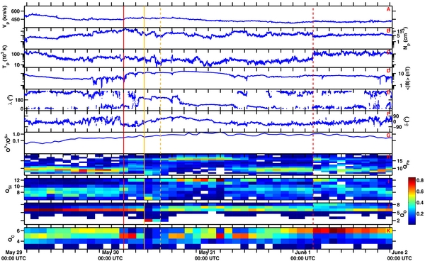
Figure 1. ACE observations of the 2005 May 20 ICME. From SWEPAM, panel A shows the proton velocity (Vp), panel B shows the proton density (Np), and panel C shows the proton temperature (Tp). From MAG, panel D shows the magnetic field magnitude (|B|), panel E shows the RTN longitude (λ), and panel F shows the RTN latitude (δ). From SWICS, panel G shows the O7 +/O6 + ratio. The final four panels, H, I, J, and K, show the charge state distributions of iron, silicon, oxygen, and carbon, respectively. The ICME plasma field begins with the solid red line at 0300 UTC on May 20 and ends with the dashed red line at 0200 UTC on May 22, where these boundaries were determined by Richardson & Cane (2010). The cold plasma observation begins with the solid yellow line, at 0808 UTC on May 20, and ends with the dashed yellow line, at 1208 UTC on May 20. These boundaries were determined by Lepri & Zurbuchen (2010).
Download figure:
Standard image High-resolution imageAs seen in Figure 1, the plasma composition during the ICME is much different from that of nominal solar wind observations. It has been previously discussed that hot charge states are closely associated with ICME plasma observations (Lepri et al. 2001; Henke et al. 2001; Richardson & Cane 2004). This behavior can be seen in the plasma composition of the 2005 May 20 ICME observation, as the average iron charge state moves from Fe+9 to a hotter distribution with a significant contribution from Fe16 +. Additionally, oxygen and silicon charge states show signs of elevated coronal temperatures as each species becomes more ionized. The O7 +/O6 + ratio is elevated during this time period and Si12 + becomes dominant, which is the maximum observable charge state for silicon. During the time period marked by the vertical solid magenta lines the plasma composition exhibits very low charge states indicating cold electron temperatures in the freeze-in region. Here the peak charge states drop from C6 +, O7 +, and Fe16 + to C2 +, O2 +, and Fe7 +, respectively.
We now attempt to reproduce these low charge state observations with differing types of simulations. We first test whether the observed ionic charge state signatures can be reproduced by a single plasma undergoing a complicated expansion history. In a first representative model, initial heating followed by adiabatic cooling for the CME will give rise to lower charge states; however, the plasma is not able to produce a significant contribution of hot plasma. A second model will assume that the observed distributions are the product of two plasmas with distinctly different temperature histories, akin to a prominence and cloud plasma, respectively.
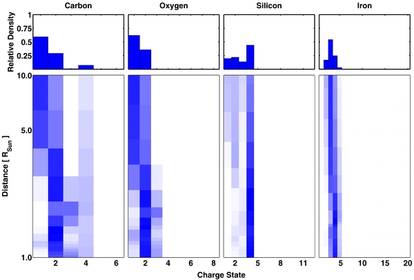
The resulting charge state distribution after freeze-in of each of these simulations are compared to our ACE/SWICS observations. Our goal is not to quantitatively match all observations, but to obtain qualitative agreements with observed characteristics. To achieve this, we will score each models' ability to reproduce the ACE/SWICS observations based on their abilities to match a number of key and defining features of the ICME observation: for carbon, we will look for peaks around C2 + and C4 +; for oxygen, we look for two peaks, one around O2 + and one at the helium like O6 +; for silicon, we only look for one peak around Si6 + and a broad overall distribution extending toward higher states; for iron, we look for two peaks, one around Fe7 + and one for Fe16 +. The scores for each model result are cataloged in Table 1. A score of 1 indicates that the model was able to recreate the feature while a score of 0 indicates that the model was not.
Table 1. Summary of the Different Models' Reproduction of the 2005 May 20 ACE/SWICS ICME Observation
| Feature | Model 1 | Model 2 | Model 3 | Model 4 |
|---|---|---|---|---|
| C: peak at 2+ | 0 | 1 | 1 | 1 |
| C: peak at 4+ | 1 | 1 | 1 | 1 |
| O: peak at 2+ | 0 | 1 | 1 | 1 |
| O: peak at 6+ | 1 | 0 | 1 | 1 |
| Si: peak at ∼7 + | 1 | 1 | 1 | 1 |
| Broad Si distribution | 1 | 0 | 1 | 1 |
| Fe: peak at ∼7 + | 1 | 0 | 1* | 1 |
| Fe: peak at ∼16 + | 1 | 0 | 1 | 1 |
| Total | 6 | 4 | 8* | 8 |
Notes. A score of 1 is given if the feature is present; otherwise, a score of 0 is given. Model 1 uses a single hot plasma. Model 2 uses a single cold-dense plasma. Model 3 uses both the cold and hot plasma combined with a single mixing ratio. Model 4 uses both the cold and hot plasma combined with a mass-dependent mixing ratio. The Fe7 + peak test for model 3 has an asterisk because there is an equally large peak at Fe5 + whereas ACE/SWICS shows the coldest peak at Fe7 +.
Download table as: ASCIITypeset image
3. SINGLE PLASMA SIMULATIONS
We first attempt to create the observed charge state distributions using a single plasma, assuming that the unusually cold charge states are a byproduct of the adiabatic cooling of the ICME. The electron temperature and density profiles are shaped similarly to those from the Gruesbeck et al. (2011) study; a plasma is initially heated very rapidly and then cools as it expands. The red curves in Figure 2 show the input electron profile which resulted in the closest qualitative match between the model results and the ACE/SWICS observations. Only the first 20 RSun is shown, since the charge state distribution for all the atomic species is frozen-in entirely within this region and do not change at larger heliocentric radii. The top panel shows the electron density profile, the middle panel shows the electron temperature, and the bottom panel shows the bulk flow velocity of the plasma. The density and temperature are related to each other adiabatically, as was shown in Gruesbeck et al. (2011). A hot, dense plasma was simulated first, with a maximum temperature of 2.6 × 10⁶ K and the maximum density of 2.4 × 1010cm−3. The velocity profile is determined by the linear acceleration calculated from height–time plots observed by SOHO/LASCO (St. Cyr et al. 2000) and the 1 AU velocity of the ICME, as observed by ACE. Figure 3 shows the initial charge state distribution of the modeled plasma using an electron temperature of 1 × 10⁴ K, along row B, compared to ACE/SWICS observations from the 2005 May 20 ICME, along row A. Figure 4 shows the evolution of the charge state distribution during the first 10 RSun of the plasmas propagation. We see that the plasma reacts to the rapid increase of the electron temperature very quickly. Within the first 1–5 RSun the charge states are seen to be frozen-in, with the lightest elements freezing earlier.

Figure 2. Input parameters for the freeze-in code for the multiple plasma simulation over the first 20 RSun. The top panel shows the electron density. The middle panel shows the electron temperature. While the bottom panel shows the bulk velocity, constrained from the linear acceleration plots from SOHO/LASCO observations for the 2005 May 20 ICME (St. Cyr et al. 2000). The cold plasma is denoted by the blue line while the hotter plasma is in red. Only one velocity curve is shown, as both plasmas use the same profile.
Download figure:
Standard image High-resolution image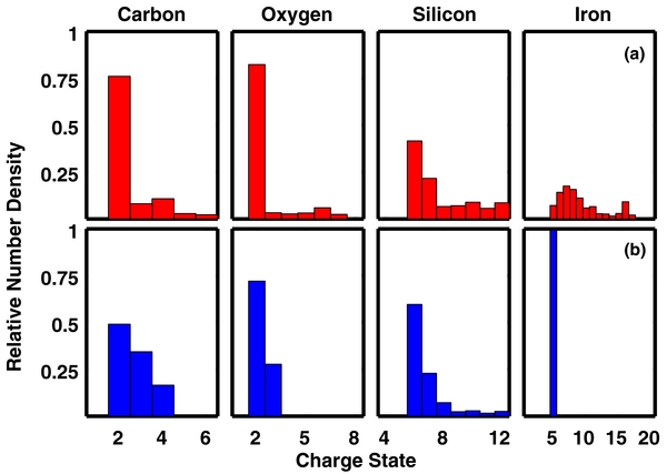
Figure 3. Comparison of ACE/SWICS charge state distribution and the initial charge state distribution for the modeled plasma. Row A shows the ACE/SWICS observations from the 2005 May 20 ICME. Row B shows the initial charge state distribution used for each modeled plasma.
Download figure:
Standard image High-resolution image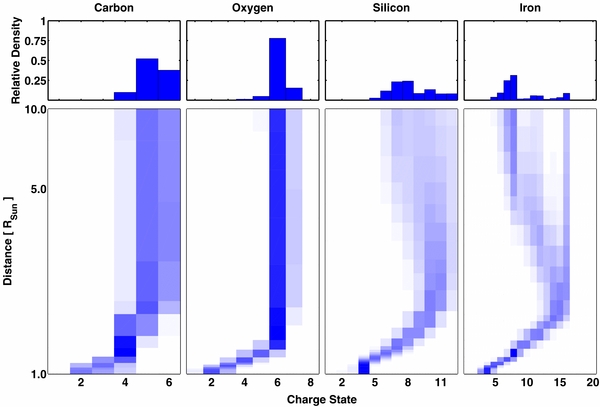
Figure 4. Result from the charge state evolution model using a hot, dense plasma for each of the atomic species modeled. Bottom row shows the evolution of the charge state distribution during the first 10 RSun after ejection. The top row shows the resulting 1 AU charge state distribution.
Download figure:
Standard image High-resolution imageIn Figure 5, we show a comparison of the model results, along row B, to a low charge state plasma observation of the ICME at ACE, along row A. Each column represents a different atomic species. Going from left to right we show carbon, oxygen, silicon, and iron. The model does replicate some of the features of the observation. Notably, we see the higher carbon and oxygen peaks of C4 + and O6 + as well as peaks in iron around Fe7 + and Fe16 +. In silicon we see a broad distribution and a peak near Si6 +. What are not reproduced are the cold charge states of carbon and oxygen, which are present in the ACE/SWICS observation. Table 1 summarizes the result of the eight qualitative tests for this simulation under the model 1 column. This simulation was able to reproduce six of the eight features we highlighted, primarily lacking at recreating the cold lower mass ions.
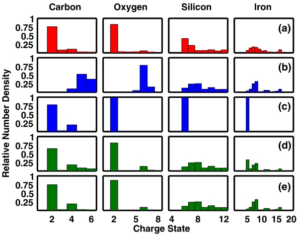
Figure 5. Comparison of ACE/SWICS charge state distribution and the charge state evolution model results, at 1 AU, for the four different atomic species, carbon, oxygen, silicon, and iron. Row A shows the ACE/SWICS observations from the 2005 May 20 ICME. Row B shows the model result of a single hot plasma. Row C shows the model result from a single cold-dense plasma. Row D shows a combination of the hot and cold plasma model results using a single mixing ratio. Row E shows a combination of the hot and cold plasma model results using a mass-dependent mixing ratio.
Download figure:
Standard image High-resolution imageIonic charge states are known to freeze in closer to the Sun for lower mass species (Hundhausen 1972; Buergi & Geiss 1986; Geiss et al. 1995). For example, Hundhausen (1972) states that the oxygen charge state freezes in around 1.2 RSun while the iron charge state freezes in further from the corona, between 2 and 3 RSun, with an ordering that remains even with more rapid expansion (Geiss et al. 1995). In this simulation, the low-mass species froze-in while the plasma was still very hot. The plasma was dense enough to allow ample cooling of the higher mass species resulting in the broader distribution of silicon and iron. Even during the abnormally cool iron charge state observations, there is often still a population of hotter Fe16 +, as can be seen in Figure 5.
A colder-dense single plasma simulation was also conducted in an attempt to reproduce the anomalously cool low-mass charge states. The electron temperature and density profiles are shaped similarly as the previous case, however the temperature maximum is considerably cooler, with a temperature of 1 × 10⁵ K, while the density maximum is greater, with a density of 9.5 × 1010 cm−3. This temperature range is consistent with the analysis of Gilbert et al. (2012). The dashed blue curve in Figure 2 shows the input electron density and temperature profiles, in panels A and B, respectively. The velocity profile is identical to the previous simulation and lies along the red curve in panel C. The cold plasma is initialized with the same temperature and charge state distribution as the hot plasma model. Figure 6 shows the evolution of the charge state distribution in the low solar atmosphere. The charge state distribution stays close to the initial state while the plasma approaches the maximum temperature. Afterward, the ions begin to transition to even colder states than initially present before freezing in.
Figure 6. Result from the charge state evolution model using a colder-dense plasma for each of the atomic species modeled presented similar to Figure 4.
Download figure:
Standard image High-resolution image
Row C of Figure 5 shows the result of the colder single plasma simulation. In all four species, we see much colder distributions than previously seen in the hotter plasma simulation along row B. Qualitatively, the carbon distribution looks similar to the ACE/SWICS observation. A peak at C2 + and a minor peak at C4 + are both observed in the resulting model distribution. Additionally, the cold peaks of O2 + and Si6 + are also recreated in the model. However, the distributions for oxygen, silicon, and iron are too cold compared to the ACE/SWICS observations. The model fails to recover the observed peak at O6 +, and the silicon and iron distributions are much too cold. It is important to remember that the charge state distribution range for the model results, plotted in Figure 5, is constrained to the charge states that are resolved in the triple-coincidence measurements from ACE/SWICS. The model results may have densities in colder charge states; however, due to this constraint the plots in row C show only density in charge state bins resolved in the ACE/SWICS data set. Recently, Gilbert et al. (2012) have shown that in these cold charge state ICME events, singly charged ions are present in double-coincidence ACE/SWICS observations, consistent with the colder ions the model produces. Presently, only the triple-coincidence data set will be considered. Table 1 summarizes the result of the eight qualitative tests under the model 2 column. This simulation only recreated four of the eight features, lacking most of the hotter features.
4. MULTIPLE PLASMA SIMULATION
Following a notional model of prominence plasma mixed with hot cloud plasma, we now use a combination of two different plasma simulation results to replicate the ACE/SWICS observations. We used a hot plasma, such as one would find from flare heating associated with the eruption (Reinard 2005; Lynch et al. 2011), and a much denser but cooler plasma, such as the prominence material found in the CME core (Rouillard 2011). Figure 2 shows the input profiles for both plasma populations. These are identical plasma profiles as described in the previous section. To determine the mixing ratio we perform a linear least-square regression. This method calculates the total difference squared of the measured charge state distribution to the modeled distribution for all possible mixing ratios. We then select the mixing ratio that corresponds to the smallest difference between the observation and model. All four species were used in the solution vector to determine a single mixing ratio to reproduce the ACE/SWICS observations. The resulting mixing ratio is given in Equation (1):

The resulting combined distribution is plotted in Figure 5 in row D. Qualitatively, the multiple plasma solution is in agreement with the ACE/SWICS observations. We succeeded in reproducing low charge state carbon, oxygen, and iron concurrently with their high charge state counterparts. In the lower mass species, we are able to recreate a population of doubly charged carbon and oxygen ions while concurrently having a hotter population of carbon around 4 + and oxygen around 6 +. Table 1 shows the results of the features we aim to replicate. The single mixing ratio simulation's scores are shown under the model 3 column. This model is able to reproduce all eight features, however, there is one major discrepancy in the reproduced charge states and those that are observed. Near the colder peak in the iron distribution we see that there are two noticeable populations. One is near Fe7 +, the peak location we are attempting to reproduce, while the other is at Fe5 + which is the location of the cutoff for the triple-coincidence data set. This particular mixing ratio is causing an overabundance of cold plasma to occur in the iron distribution. We interpret this to be caused by compositional differences between prominence and cloud-type data.
To test this assumption, mixing ratios for each species were determined using a linear least-squares regression like before, but solving for mixing ratios for each species. Table 2 shows the mixing ratios we determined for each species. Due to the small charge state distribution range observable by ACE/SWICS for silicon, the majority of the modeled cold plasma falls in charge states not delivered in the triple-coincidence data. Therefore, the mixing ratio of iron is used for silicon. Row E in Figure 5 shows the resulting charge state distribution using the species-dependent mixing ratios. Comparing the resulting charge state distribution to that of the ACE/SWICS observations we see a very good qualitative match. All eight of the features we are scoring are recreated in this model's resulting distribution like in the previous single mixing ratio text. A summary of the scores from our qualitative test is shown in Table 1 under the model 4 column. The cold iron peak no longer shows two populations, like the previous case. Now, only the peak near Fe7 + remains consistent with our data.
Table 2. Mixing Ratio Determined for Each Species
| Species | Cold Plasma Contribution | Hot Plasma Contribution |
|---|---|---|
| Carbon | 0.983 | 0.017 |
| Oxygen | 0.955 | 0.045 |
| Silicon | 0.104 | 0.896 |
| Iron | 0.104 | 0.896 |
Notes. The majority of the cold plasma modeled for silicon lies outside of the range of silicon charge states resolved for ACE/SWICS, therefore a mixing ratio is not able to be calculated. The mixing ratio determined for iron is used for silicon as well.
Download table as: ASCIITypeset image
5. DISCUSSION
In the previous sections, we have shown that we can qualitatively recreate the observations of anomalously low charge state plasma from the 2005 May 20 ICME. Our first attempts involved modeling two different single plasma to test if the cold ion observations were a byproduct of the adiabatic cooling of the ICME as it expands into the heliosphere. We ran a variety of cold and hot models, with a range of expansion profiles, with a result: models based on the temperature history of one single plasma cannot produce concurrent hot and cold signatures, as observed.
This result is not entirely surprising when considering the ionization timescales for different mass ions. During its expansion into space, a given ion freezes in once its ionization timescale becomes greater than its expansion timescale. Lower mass species tend to freeze in closer to the corona, with the freeze-in distance moving outward as the mass of the species increases (Geiss et al. 1995; Buergi & Geiss 1986). In our ICME simulation, the presence of hot plasma requires heating very early on in the plasmas expansion history. In this case, carbon and oxygen charge state distributions freeze in while the ICME plasma is still heating and therefore reflect these high temperatures. Furthermore, the plasma density may be large enough to allow the heavier species to recombine further out, relaxing into lower and cooler charge states, but successively losing high charge state signatures. Thus, we can conclude that low ionic charge state plasma seen in all four species in ICMEs cannot result strictly from expansion effects on a single plasma population. Similarly, in the case of the single cold case, the plasma never experiences a hot enough environment to produce ions in the higher charge states, such as those observed in the ICME observation.
We therefore conclude that our observations are reflective of the multi-temperature nature of CMEs observed at the Sun (House et al. 1981): cold ionic charge states originate in cool and dense prominence plasma. Hotter charge states come from cloud plasma that is magnetically dominated. Combining these two solutions, we are able to qualitatively match the ACE/SWICS behavior in all four elements. These two plasma contributions mix during their heliospheric expansion, suggesting that prominence and cloud plasma are on the same field lines in the corona, providing an important clue for the magnetic structure and relation of prominence plasmas and CME.
Prominences have been described as an important part of the initiation process of CMEs. One model suggests that prominences can act as an anchor, preventing the bent magnetic flux rope from ejecting (Low 1999; Low et al. 1982). As plasma drains from prominences under gravitational pull, the magnetic forces on the flux rope in the corona are no longer balanced forcing the CME to erupt, dragging the magnetically attached prominence with it (Low et al. 2003). Through this process, prominences can lose ∼90% of their mass (Schmahl & Hildner 1977) as the material drains from the loops into the corona. Despite this the prominence plasma is still a significant portion of the ICME, accounting for an average of ∼20% of the mass of the ejecta (Gilbert et al. 2006). However, this model does not predict a mixing of the hot and cold plasma. During the eruption, a helmet streamer loop is ejected as the internal flux rope is propelled outward. The reconnection occurs low in the corona, to close the streamer loop, but does not necessarily connect the streamer field lines with the internal flux rope where the prominence is confined.
In prominence models by Karpen et al. (2001) and Aulanier et al. (2000), prominences form around a neutral line where the surrounding magnetic field is highly sheared. The breakout model of Antiochos et al. (1999) requires a similar magnetic configuration. They propose a multiflux system with neutral lines at the boundaries of sheared flux arcades. Prominence plasma is then confined in the regions along these neutral lines, called filament channels. As breakout reconnection occurs, the magnetic field of the closed corona can reconnect with the filament channel, placing prominence plasmas on the same field lines as the flux ropes that are being formed as part of the reconnection process (Lynch et al. 2004). This is consistent with our observations, which show that prominence and flux-rope plasmas are on the same field lines and can therefore mix.
Finally, we have shown that the best match of our model with our observations occurs when each species experiences a different mixing ratio. Table 2 shows the mixing ratios that we used. As can be seen, the lower mass species of carbon and oxygen are composed primarily of the cold prominence material while the heavier species, iron, is primarily composed of the hot leading edge plasma with a very small amount of prominence material. Gravitational forcing will act stronger on these heavier species than the lighter ones. Countering the forcing from gravity, the plasma also experiences collisional drag, from ions traveling along the magnetic field from the corona. However, for heavier species the gravitational force dominates the force from collisional drag. Gilbert et al. (2002) calculated the draining timescales for both hydrogen and helium in a prominence assuming both of these forces were acting on the plasma. They found that the heavier helium drains much more quickly than hydrogen. This is consistent with our resulting ICME observation. The charge state distribution of the lighter species is comprised of a larger percentage of prominence material than the heavier species.
This work was supported, in part, by the NASA Graduate Student Research Program grant NNX10AM41H, the ACE mission 44A-1085637 and NASA grants NNX07AB99G and NNX10AQ61G. We used the SOHO/LASCO CME catalog developed by NASA, NRL and the Catholic University of America. SOHO is a project of international cooperation between ESA and NASA. This work was performed, in part, with support from the GSRP program. The authors thank Enrico Landi for early discussions which helped to foster this study.