


ABSTRACT
We have finally measured the evolutionary rate of cooling of the pulsating hydrogen atmosphere (DA) white dwarf ZZ Ceti (Ross 548), as reflected by the drift rate of the 213.13260694 s period. Using 41 yr of time-series photometry from 1970 November to 2012 January, we determine the rate of change of this period with time to be dP/dt = (5.2 ± 1.4) × 10−15 s s−1 employing the O − C method and (5.45 ± 0.79) × 10−15 s s−1 using a direct nonlinear least squares fit to the entire lightcurve. We adopt the dP/dt obtained from the nonlinear least squares program as our final determination, but augment the corresponding uncertainty to a more realistic value, ultimately arriving at the measurement of dP/dt = (5.5 ± 1.0) × 10−15 s s−1. After correcting for proper motion, the evolutionary rate of cooling of ZZ Ceti is computed to be (3.3 ± 1.1) × 10−15 s s−1. This value is consistent within uncertainties with the measurement of (4.19 ± 0.73) × 10−15 s s−1 for another similar pulsating DA white dwarf, G 117-B15A. Measuring the cooling rate of ZZ Ceti helps us refine our stellar structure and evolutionary models, as cooling depends mainly on the core composition and stellar mass. Calibrating white dwarf cooling curves with this measurement will reduce the theoretical uncertainties involved in white dwarf cosmochronometry. Should the 213.13 s period be trapped in the hydrogen envelope, then our determination of its drift rate compared to the expected evolutionary rate suggests an additional source of stellar cooling. Attributing the excess cooling to the emission of axions imposes a constraint on the mass of the hypothetical axion particle.
Export citation and abstract BibTeX RIS
1. INTRODUCTION
ZZ Ceti (Ross 548) is the prototype of the class of hydrogen atmosphere variable (DAV) white dwarfs that are pulsationally unstable in the temperature range 10,800–12,300 K for log g ≈ 8 (Koester & Holberg 2001; Bergeron et al. 2004; Gianninas et al. 2005, 2006). The ZZ Ceti stars constitute the coolest class of pulsating white dwarfs, with more than 150 members known to date (e.g., Mukadam et al. 2004; Kepler & Castanheira 2009; Castanheira et al. 2010; Greiss 2012).
The pulsation characteristics of the hot ZZ Ceti stars closer to the blue edge of the instability strip are different from their compatriots near the red edge. The distinct behavior of pulsation periods, amplitudes, and degree of amplitude modulation as a function of temperature was demonstrated for a significant sample of DAVs by Clemens (1993) and more recently by Kanaan et al. (2002) and Mukadam et al. (2006, 2007). Cool ZZ Ceti stars typically show relatively longer pulsation periods around 650–1000 s, larger amplitudes (up to 30%), nonlinear pulse shapes, and greater amplitude modulation (e.g., Kleinman et al. 1998). The hot ZZ Ceti stars show relatively few pulsation modes, shorter periods around 100–350 s with low amplitudes (∼0.1%–3%), and only a small degree of amplitude modulation (Clemens 1993; Mukadam et al. 2006, 2007). Typical of the class of hot DAV pulsators, ZZ Ceti exhibits short periods at 187 s, 213 s, 274 s, 318 s, and 334 s with amplitudes in the range of 0.5–6.6 mma.16 The pulsation spectrum of ZZ Ceti exhibits a very low degree of amplitude modulation over decades, making it possible to measure the miniscule change of its pulsation period over that timespan to arrive at the rate of change of period with time, dP/dt.
Pulsation periods of model white dwarf stars increase as the star cools due to the increasing radius of the degeneracy boundary (Winget et al. 1983). Gravitational contraction decreases the periods, but is found to be very small in the temperature range of the ZZ Ceti instability strip compared to the hotter classes of pulsating white dwarfs (Kepler et al. 2000). Although this implies that the rate of change of period with time dP/dt is governed by the rate of stellar cooling for the ZZ Ceti stars (Kepler et al. 2000), eigenmodes trapped in the outer hydrogen envelope (e.g., 213 s) are still expected to show reduced values of dP/dt due to first order effects from residual gravitational contraction.
2. NEW OBSERVATIONS OF ZZ Ceti FROM 2002 TO 2012
Since the last publication of this work in a refereed journal (Mukadam et al. 2003), we have obtained ten more years of time-series photometry on ZZ Ceti. Most of these data were obtained at the 2.1 m Otto–Struve telescope at McDonald Observatory with the time-series charge-coupled device (CCD) photometer named Argos (Nather & Mukadam 2004). The journal of observations of these data is given in Table 5. We have not included data obtained in marginal weather or that which was discarded due to timing problems.
Almost all the data were acquired with the wide band Schott glass BG 40 filter. Pulsation amplitudes are a function of wavelength (Robinson et al. 1995); unfiltered observations of ZZ Ceti stars yield amplitudes reduced by as much as 35%–42% compared to BG 40 photometry that suppresses the red wavelengths (Kanaan et al. 2000; Nather & Mukadam 2004).
We used a standard IRAF reduction (Tody 1993) to extract sky-subtracted light curves from the CCD frames using weighted circular aperture photometry (O'Donoghue et al. 2000). After a preliminary reduction, we brought the data to a fractional amplitude scale (Δ I/I) and converted the mid-exposure times of the CCD images to barycentric dynamic time. We also subtracted a low order best-fit polynomial (at the timescale of several hours) from lightcurves that showed residual extinction effects. Last, we computed a discrete Fourier transform (DFT) of the individual nightly runs as well as the combined data from closely spaced runs.
The 2007 August data set constitutes the highest signal-to-noise observations that we have acquired on ZZ Ceti, albeit the 2011 December–2012 January data set is also close in data quality. Table 1 lists the results of a nonlinear least squares fit to all the periodicities (above 3σ) in the 2007 lightcurve obtained using the program Period04 (Lenz & Breger 2005).
Table 1. High Signal-to-noise 2007 August ZZ Ceti Data Yield the Best-fit Periodicities Shown with the Listed Least Squares and Italicized Monte Carlo Uncertainties Computed using Period04
| Frequency | Period | Amplitude |
|---|---|---|
| (μHz) | (s) | (mma) |
| 4691.8904 ± 0.0055 | 213.13371 ± 0.00025 | 6.587 ± 0.070 |
| ± 0.0057 | ± 0.00026 | ± 0.082 |
| 4699.8685 ± 0.0090 | 212.77191 ± 0.00041 | 4.293 ± 0.069 |
| ± 0.011 | ± 0.00050 | ± 0.079 |
| 4696.006 ± 0.031 | 212.9469 ± 0.0014 | 1.191 ± 0.069 |
| ± 0.034 | ± 0.0015 | ± 0.075 |
| 3646.2442 ± 0.0086 | 274.25481 ± 0.00065 | 4.129 ± 0.065 |
| ± 0.010 | ± 0.00077 | ± 0.078 |
| 3639.321 ± 0.011 | 274.77652 ± 0.00087 | 3.146 ± 0.069 |
| ± 0.013 | ± 0.00097 | ± 0.076 |
| 3642.694 ± 0.032 | 274.5221 ± 0.0024 | 1.206 ± 0.066 |
| ± 0.035 | ± 0.0027 | ± 0.078 |
| 3143.835 ± 0.038 | 318.0829 ± 0.0039 | 0.822 ± 0.061 |
| ± 0.043 | ± 0.0043 | ± 0.067 |
| 2997.250 ± 0.038 | 333.6392 ± 0.0042 | 0.830 ± 0.061 |
| ± 0.050 | ± 0.0056 | ± 0.073 |
| 5351.703 ± 0.063 | 186.8564 ± 0.0022 | 0.502 ± 0.061 |
| ± 0.073 | ± 0.0025 | ± 0.069 |
Download table as: ASCIITypeset image
Figure 1 shows the DFT of the 2007 lightcurve (top panel) with a 3σ level of 0.45 mma. The middle panel shows the DFT obtained after subtracting the periods listed in Table 1, but only two components from the 213 s and 274 s multiplets. There is considerable residual power above the 3σ line, which implies the presence of another component. We show the prewhitened DFT obtained after the subtraction of all three periods of the 213 s and 274 s modes (bottom panel). This demonstrates that the 213 s and 274 s multiplets are indeed triplets; Mukadam et al. (2003) were unable to prove or disprove the existence of the third low-amplitude component of these multiplets before. Although it was possible to fit the third component in previous data, prewhitening led to an increase in the background noise, making the detection of the third component ambiguous.

Figure 1. Discrete Fourier transform (DFT) of the 2007 August data on ZZ Ceti is shown in the top panel. The middle panel shows the prewhitened DFT obtained after subtracting two components of the 213 s and 274 s multiplets, as well as the 187 s, 318 s, and 334 s modes. The bottom panel shows the effect of additionally subtracting out the third low-amplitude component of the 213 s and 274 s triplets.
Download figure:
Standard image High-resolution imageCuriously, ZZ Ceti ended up being the DAV class prototype as it was the first DAV believed to be deciphered, even though it was the third ZZ Ceti star to be discovered after HL Tau76 and G 44-32. We have uncovered the triplet nature of the 213 s and 274 s modes only recently (Mukadam et al. 2009), and still not satisfactorily resolved the other low-amplitude multiplets. There is an indication of splitting even in the 187 s and 334 s modes, visible as residual power left behind in the bottom panel of Figure 1. We will address this in the next section.
3. UNIQUE MODE IDENTIFICATION
There are presently two distinct sets of mode indices in the literature for the observed pulsation spectrum of ZZ Ceti. Bischoff-Kim et al. (2008a) identify the 213 s, 274 s, and 318 s modes as ℓ = 1, k = 1, 2, and 4, respectively, while concluding that the 187 s and 334 s modes are ℓ = 2 modes with k = 4 and k = 8. Romero et al. (2012) fit the 187 s, 213 s, and 274 s modes to be ℓ = 1, k = 1, 2, and 3, respectively, while identifying the 318 s and 334 s modes as ℓ = 2 with k = 8 and k = 9. Constraining the splitting of either the 187 s or the 318 s mode would be useful in eliminating one model in favor of another and obtaining a unique mode identification for ZZ Ceti.
In the absence of high signal-to-noise multi-site observations,17 required to resolve these low-amplitude multiplets, we resorted to a nonlinear least squares analysis of a 4.5 yr lightcurve from 2007 August to 2012 January. Although we achieve high signal-to-noise due to the timespan of the lightcurve, these data have large gaps and are essentially single-site. Consequently, it is difficult to distinguish between the true frequencies and aliases. Figure 2 shows the DFT obtained from the 4.5 yr long lightcurve, while Table 2 shows the best-fit periodicities with both least squares and Monte Carlo uncertainties. It is with a grain of salt that we present the individual components of the low-amplitude multiplets, especially the expected quintuplet at 334 s. With future high signal-to-noise multi-site data, it should be possible to resolve these multiplets with less ambiguity.
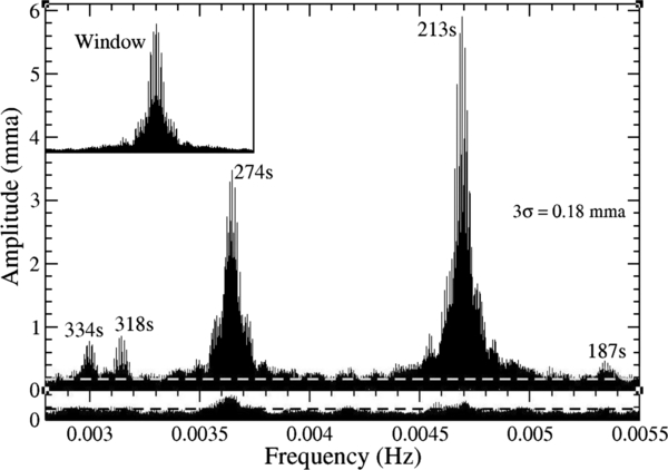
Figure 2. DFT of a 4.5 yr ZZ Ceti lightcurve from 2007 August to 2012 January is shown in the top panel, while the bottom panel with the same y-scale shows the prewhitened DFT.
Download figure:
Standard image High-resolution imageTable 2. ZZ Ceti Data from 2007 August to 2012 January Lead to the Best-fit Periodicities Shown Against their Mode Identification from Romero et al. (2012)
| ℓ | k | m | Frequency | Period | Amplitude | δσrot | Ck, ℓ | Prot |
|---|---|---|---|---|---|---|---|---|
| (μHz) | (s) | (mma) | (μHz) | (days) | ||||
| 1 | 1 | −1 | 5351.72234 ± 0.00024 | 186.8557329 ± 0.0000085 | 0.482 ± 0.044 | 5.05686 ± 0.00046 | 0.381 | 1.42 |
| ± 0.00036 | ± 0.000013 | ± 0.051 | ± 0.00053 | |||||
| 1 | 1 | 0 | 5356.00247 ± 0.00031 | 186.706411 ± 0.000011 | 0.391 ± 0.044 | |||
| ± 0.00022 | ± 0.0000076 | ± 0.040 | ||||||
| 1 | 1 | +1 | 5361.83606 ± 0.00039 | 186.503278 ± 0.000014 | 0.303 ± 0.043 | |||
| ± 0.00026 | ± 0.0000092 | ± 0.063 | ||||||
| 1 | 2 | −1 | 4691.914514 ± 0.000018 | 213.1326129 ± 0.00000083 | 6.551 ± 0.044 | 4.015327 ± 0.000032 | 0.494 | 1.46 |
| ± 0.000026 | ± 0.0000012 | ± 0.030 | ± 0.000039 | |||||
| 1 | 2 | 0 | 4695.93033 ± 0.00012 | 212.9503484 ± 0.0000055 | 0.997 ± 0.044 | |||
| ± 0.0073 | ± 0.00033 | ± 0.15 | ||||||
| 1 | 2 | +1 | 4699.945167 ± 0.000027 | 212.7684397 ± 0.0000012 | 4.354 ± 0.044 | |||
| ± 0.000029 | ± 0.0000013 | ± 0.061 | ||||||
| 1 | 3 | −1 | 3639.348197 ± 0.000036 | 274.7744777 ± 0.0000027 | 3.223 ± 0.044 | 3.473157 ± 0.000046 | 0.374 | 2.09 |
| ± 0.000035 | ± 0.0000026 | ± 0.29 | ± 0.0072 | |||||
| 1 | 3 | 0 | 3642.68971 ± 0.00017 | 274.522421 ± 0.000012 | 0.705 ± 0.043 | |||
| ± 0.0020 | ± 0.00015 | ± 0.096 | ||||||
| 1 | 3 | +1 | 3646.294510 ± 0.000028 | 274.2510231 ± 0.0000021 | 4.153 ± 0.044 | |||
| ± 0.0072 | ± 0.00054 | ± 0.54 | ||||||
| 2 | 8 | −2 | 3132.74663 ± 0.00029 | 319.208706 ± 0.000030 | 0.435 ± 0.049 | 5.56333 ± 0.00046 | 0.152 | 1.76 |
| ± 0.00024 | ± 0.000025 | ± 0.10 | ± 0.00047 | |||||
| 2 | 8 | 0 | 3143.83187 ± 0.00035 | 318.083168 ± 0.000035 | 0.393 ± 0.049 | |||
| ± 0.42 | ± 0.043 | ± 0.11 | ||||||
| 2 | 8 | +2 | 3154.99996 ± 0.00036 | 316.957215 ± 0.000036 | 0.363 ± 0.044 | |||
| ± 0.00037 | ± 0.000037 | ± 0.070 | ||||||
| 2 | 9 | 2974.38897 ± 0.00039a | 336.203506 ± 0.000044 | 0.324 ± 0.048 | 0.133 | |||
| ± 0.047 | ± 0.0053 | ± 0.051 | ||||||
| 2 | 9 | 2982.00312 ± 0.00043a | 335.345055 ± 0.000049 | 0.279 ± 0.044 | ||||
| ± 0.00064 | ± 0.000072 | ± 0.065 | ||||||
| 2 | 9 | 2989.62272 ± 0.00036a | 334.490366 ± 0.000040 | 0.332 ± 0.045 | ||||
| ± 0.014 | ± 0.0016 | ± 0.092 | ||||||
| 2 | 9 | 2997.20401 ± 0.00023a | 333.644289 ± 0.000025 | 0.563 ± 0.047 | ||||
| ± 0.070 | ± 0.0078 | ± 0.14 | ||||||
Notes. Formal least squares and italicized Monte Carlo uncertainties computed using Period04 are also shown. The implied rotation periods determined from the multiplet spacings are listed, with bold values obtained from the high-amplitude triplets. aThe quintuplet at 334 s is not clearly resolved, and the frequency components presented here must be taken with a grain of salt. Future multi-site data should help to distinguish the aliases from the true frequencies without ambiguity.
Download table as: ASCIITypeset image
The 187 s mode is a triplet with a spacing of 5.05686 μHz, consistent with an ℓ = 1 identification. The equations in the subsequent section will show that the larger spacing of the 187 s triplet compared to the 213 s triplet can be accounted for by the correspondingly smaller value of the rotational co-efficient Ck, ℓ. The observed spacing of the 318 s mode necessitates its identification as an ℓ = 2 mode, also inconsistent with the deduced mode identification presented by Bischoff-Kim et al. (2008a). The splittings we obtain are completely consistent with the mode identification of Romero et al. (2012), also indicated in Table 2.
4. ROTATION PERIOD
With the loss of spherical symmetry arising from both stellar rotation and a magnetic field, a pulsation mode can be expected to show an uneven multiplet splitting given by the following equations (see Hansen et al. 1977; Brassard et al. 1989; Jones et al. 1989; Winget et al. 1994; Winget & Kepler 2008):


where σk, l, m is the observed frequency dependent on the radial (k), azimuthal (ℓ), and magnetic (m) mode indices, σk, l is the unperturbed frequency, Ck, l is the rotational coefficient, Ω gives the frequency of rotation, D is a constant, and B is the magnetic field strength. The 213 s and 274 s triplets are rotationally split ℓ = 1 modes with the uneven spacing, implying the presence of a magnetic field. Following the formalism of Winget et al. (1994), we can compute the rotational and magnetic components of the splitting as given by the following equations:


The best-fit asteroseismological model of Romero et al. (2012) for ZZ Ceti yields an effective temperature of Teff = 11627 ± 390 K, stellar mass M⋆ = 0.609 ± 0.012 M☉, log g = 8.03 ± 0.05, radius log (R⋆/R☉) = −1.904 ± 0.015, and the luminosity log (L⋆/L☉) = −2.594 ± 0.025. The fractional central abundances are determined to be  and
and  with hydrogen and helium layer masses of MH = (1.10 ± 0.38) × 10−6 M⋆ and MHe = 0.0245 M⋆. We have utilized this model to obtain the values of the rotational coefficients Ck, l listed in Table 2, assuming uniform rotation.
The 213 s triplet yields a multiplet spacing of δσrot = 4.015327 ± 0.000039 μHz, implying a rotation period of Prot = 1.46 days. The 274 s mode with a rotational splitting of 3.4732 ± 0.0072 μHz gives a spin period of 2.09 days. The observational Monte Carlo uncertainty in obtaining these values is negligible, and the true uncertainty in determining the rotation period is governed solely by the error in the model values of Ck, l. Should the theoretical uncertainty in the rotational coefficients be as large as 20%, then the discrepant values of 1.46 and 2.09 days would still be consistent with solid-body stellar rotation. Otherwise, we have apparently detected preliminary evidence of differential rotation in ZZ Ceti. Note that the splittings derived for the low-amplitude multiplets at 187 s and 318 s are less reliable since we may have converged on an alias; extensive analysis of single-site data cannot replace the credibility of multi-site observations.
Although the idea of a small amount of differential rotation seems more reasonable than our simple-minded notion of rigid body rotation for as complex a system as a star, we are unable to be conclusive about this point. The model values of Ck, l adopted here were derived assuming uniform rotation, and we need to properly establish their real uncertainties. Second, we show the weight functions and rotational kernels of the ℓ = 1, k = 1, 2, and 3 modes of the best-fit model (Figure 3). The weight function reveals which region of the star a given mode is sensitive to, and the rotational kernel indicates the regions of the star that are relevant for the value of the frequency splitting (e.g., Kawaler et al. 1999; Córsico et al. 2011). Figure 3 shows that the k = 1 mode samples the triple transition region O/C/He, while the k = 2 mode samples the He/H interface of the model white dwarf. The k = 3 mode is found to sample the model He layer and is also sensitive to the chemical structure of the C/O transition region. It is possible that a small amount of accretion from a comet or a planet, for example, may have spun up the H layer to rotate slightly faster than the rest of the star, but such far-fetched hypotheses should only be explored after an accurate determination of the Ck, l values. Hence we simply present a weighted average of the values of spin period obtained from the high-amplitude 213 s and 274 s triplets, and state that the mean rotation period of ZZ Ceti is Prot = 1.7 ± 0.3 days.
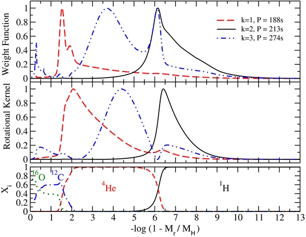
Figure 3. Weight functions and rotational kernels of the ℓ = 1, k = 1, 2, and 3 modes from the best-fit seismological model (Romero et al. 2012) are shown against the chemical composition profiles.
Download figure:
Standard image High-resolution imageWithin Monte Carlo uncertainties, the 213 s triplet is even with δσB = 0.0005 ± 0.0073 μHz, while the 274 s triplet is relatively uneven with δσB = 0.1316 ± 0.0075 μHz. It is possible that the 213 s mode is aligned with the axis of the magnetic field, and hence we do not detect any evidence of an uneven splitting. Dividing by 2π as per Jones et al. (1989), we yield a frequency splitting of Δ fm = 0.0209 ± 0.0012 μHz for the 274 s triplet. Scaling this observed splitting by a factor of (B/105)2 following Winget et al. (1994), we compute a weak magnetic field strength of the order of 14.5 kG, estimated using Figure 1 of Jones et al. (1989). Note that Mukadam et al. (2012) incorrectly determined magnetic field strengths of 28 kG and 30 kG for the 213 s and 274 s triplets based on the periods listed in Table 1, but our analysis shown in Table 2 should be much more robust.
Schmidt & Grauer (1997) used the polarimetric technique to measure the disk averaged longitudinal component of the magnetic field for ZZ Ceti, obtaining two separate measurements of 0.2 ± 8.8 kG in 1992 October and 8.5 ± 3.4 kG in 1996 December. Our order of magnitude estimate of 14.5 kG is within their 3σ non-detection limit.
5. DIRECT METHOD TO CONSTRAIN dP/dt
The drift rate of a changing period can be constrained by comparing measurements of the period at different times. This direct method is not as sensitive as the techniques described in the next two sections, but it is a useful exercise nonetheless.
The new observations listed in Table 5 consist of three new data sets, namely 2007 August, 2010 December, and 2011 December. This yields 12 seasons of ZZ Ceti data since its discovery that resolve the triplet well, namely 1970, 1975, 1980, 1986, 1991, 1993, 1999 September–October, 1999 November, 2000, 2007, 2010, and 2011. The older data from 1970 to 1986 and 1993 were acquired using 1 m class telescopes and instruments based on photo-multiplier tubes (intrinsic quantum efficiency 35%), but span 1.5–2 months in duration. The 1991 data were acquired using the 3.6 m Canada–France–Hawaii Telescope with the photometer LAPOUNE, also based on photo-multiplier tubes. The 1999 and 2000 data sets were acquired using 1–2 m class telescopes, mostly with multi-channel photo-multiplier tube photometers. The data obtained in the last decade from 2001 to 2011 have been acquired using a 2 m class telescope equipped with CCD-based time-series photometers, as reflected in the journal of observations (Table 5).
We simultaneously fit three frequencies to each of the 12 seasons of observations using the least squares program Period04 (Lenz & Breger 2005). The best-fit periods of the 213 s triplet are shown in Figure 4 as a function of time. The slopes themselves are not particularly useful, but the uncertainties in the slopes serve as upper limits to the dP/dt values. We hereby constrain dP/dt ⩽ 1.5 × 10⁻¹³ s s−1 for the 213.13 s period, dP/dt ⩽ 2.2 × 10⁻¹³ s s−1 for the 212.78 s period, and dP/dt ⩽ 7.8 × 10⁻¹³ s s−1 for the 212.95 s period, respectively.

Figure 4. We show the best-fit seasonal periods of the 213.13 s triplet as a function of time, as well as the dP/dt constraints from a linear fit.
Download figure:
Standard image High-resolution imageFigure 4 also helps us discern those data sets that may not be resolving the triplet very well, e.g., the 1991 season of observations stands out as an outlier in all three panels. This is the shortest data set on ZZ Ceti, about 5.3 days in duration. The signal-to-noise ratio of periodic data improves with the cycle count, and hence the 1.5–2 month long data sets acquired using 1 m class telescopes from 1970 to 1986 triumph over the 3.6 m 5 day 1991 data set. The 2000 seasonal data set also encompasses low coverage over its 47 day duration and has large gaps, causing it to deviate from the linear fits shown in Figure 4.
6. O − C ANALYSIS
A variable period can be discerned by comparing the observed phase O to the phase C calculated assuming a constant period. The larger the change in the period, the larger the discrepancy O − C. The longer the timebase of the observations, the larger the discrepancy O − C. The O − C technique is much more sensitive than the direct method because it has the advantage of adding up the discrepancy O − C over the entire timebase of observations consisting of numerous cycles. Neglecting higher order terms, Kepler et al. (1991) show the derivation of the following O − C equation using a Taylor series expansion of the phase of a slowly changing period

During the first stage of using the O − C method, the value of the period P improves linearly with the cycle count E as the first order term is dominant. The reference zero epoch is given by E0. Eventually, the second order term becomes important provided there is a non-zero detectable change in the period. The constraints on the value of dP/dt then become meaningful and improve with the square of the timebase.
The disadvantage of using the O − C method is the requirement to know with some confidence the cycle counts between observations. We are able to fulfill this requirement for the 213.13 s and 212.78 s periods in the pulsation spectrum of ZZ Ceti, but find ourselves unable to construct an O − C diagram for the low-amplitude 212.95 s period.
Mukadam et al. (2003) indicate that the 274 s mode is drifting at a rate two orders of magnitude faster than the evolutionary rate. A fast drift rate of ⩾10−12 s s−1 was also recently demonstrated for the 292.9 s mode of WD 0111+0018 (Hermes et al. 2013). Such behavior indicates that these modes are not useful in the context of measuring the stellar cooling rate. We will henceforth focus our efforts on just the 213.13 s and 212.78 s periods.
We simultaneously fit three fixed frequencies to each of the 12 seasons of observations using Period04 (Lenz & Breger 2005), while varying the amplitudes and phases. The observed phases were compared to the computed phases obtained for the constant periods of 213.13260694 s and 212.76843045 s. We show the discrepancy O − C obtained as a function of the cycle count or epoch E in Figure 5, as well as list these values in Table 3. A parabolic least squares fit to the O − C diagram yields the following values for the rates of change of period with time: dP/dt = (5.2 ± 1.4) × 10−15 s s−1 for the 213.13260694 ± 0.00000026 s period and dP/dt = (9.0 ± 2.0) × 10−15 s s−1 for the 212.76843045 ± 0.00000039 s period. Since the parabolic fit is not weighted, each point in the O − C diagram contributes equally to the best fit. We do not weight the fit because the two most deviant points in the O − C diagram, i.e., the 1991 and 2007 seasons, have the smallest least squares error bars and might skew the result.

Figure 5. O − C diagrams obtained for the 213.13260694 s and 212.76843045 s periods.
Download figure:
Standard image High-resolution image
Table 3. O − C Values for the 213.13260694 s and 212.76843045 s Periods
| Season | Period = 213.13260694 s | Period = 212.76843045 s | ||
|---|---|---|---|---|
| Epoch | O − C (s) | Epoch | O − C (s) | |
| 1970 | −3090303 | 3.0 ± 3.7 | −3095592 | 5.3 ± 6.6 |
| 1975 | −2361406 | −1.0 ± 1.4 | −2365448 | 5.6 ± 2.4 |
| 1980 | −1606615 | −3.1 ± 1.6 | −1609365 | 1.5 ± 2.5 |
| 1986 | −743875 | −3.6 ± 2.7 | −745148 | 2.6 ± 4.6 |
| 1991 | 0 | 0.00 ± 0.52 | 0 | 0.00 ± 0.79 |
| 1993 | 305529 | −3.01 ± 0.79 | 306052 | −1.1 ± 1.6 |
| 1999 Sep–Oct | 1180467 | −0.97 ± 0.89 | 1182488 | 1.0 ± 1.2 |
| 1999 Nov | 1205506 | −2.1 ± 1.4 | 1207570 | 0.3 ± 1.6 |
| 2000 | 1323972 | −3.0 ± 1.0 | 1326238 | −4.2 ± 1.5 |
| 2007 | 2360934 | −2.72 ± 0.84 | 2364976 | 2.2 ± 1.3 |
| 2010 | 2848509 | 2.9 ± 1.2 | 2853385 | 9.2 ± 1.7 |
| 2011 | 3002948 | 2.98 ± 0.95 | 3008088 | 10.2 ± 1.5 |
Download table as: ASCIITypeset image
The O − C diagram can be thought of as a comparison between two clocks: the stellar and atomic clocks. The true and complete uncertainty of any point in the O − C diagram comes from two independent sources: absolute uncertainty in time and relative uncertainty in time. Absolute uncertainty in time stems from how accurately we know the start-times of our observations. Relative uncertainty in time comes from the duration of our lightcurves, photometric accuracy, time resolution, etc. that decide how well we resolve the multiplet and dictate the uncertainty in period and phase. The uncertainty in period also governs the true uncertainty of a point in the O − C diagram, with both an explicit (uncertainty in C) and an implicit (uncertainty in O) dependence. The deviation of the 1991 data point in Figure 4 indicates that the triplet is not well resolved in this season, making the phases slightly unreliable. This is not reflected in the formal least squares error bar in the O − C diagram, because the beat phase dominates over the phase of the individual mode in a short lightcurve. Also, these data were acquired with a photo-tube photometer, where the clock is typically manually adjusted to GPS time. Skillful observers can achieve a synchronization that is better than a second; the net contribution of manual timing toward an absolute error in time reduces over several nights. Without the 1991 data, the parabolic O − C fit changes from dP/dt = (5.2 ± 1.4) × 10−15 s s−1 to (6.2 ± 1.2) × 10−15 s s−1 for the 213.13260694 s period. Eliminating a discrepant point from the fit reduces the error bar as expected, but both values are consistent with each other within the uncertainties.
The 2007 seasonal observations are more worrisome; these were acquired at the 2.1 m Otto–Struve telescope at McDonald Observatory using a CCD time-series photometer, Argos. Figure 4 reflects that the triplet is well resolved, better than other data sets from 1993 or 2000, for example. Argos has an efficient timing design, where GPS pulses directly trigger both the start and end of each exposure (Nather & Mukadam 2004). We conducted multiple timing checks with the observatory GPS clock every night during the observing run. It is not possible to ascertain the absolute error in time after the fact, but having found nothing amiss, we expect it to be of the order of a millisecond. We are therefore stumped by why the 2007 data point should be so deviant from the fit, even if it is only by a couple of seconds. If we do eliminate both the 1991 and the 2007 data points, the parabolic O − C fit changes to dP/dt = (6.50 ± 0.72) × 10−15 s s−1 with an artificial reduction in uncertainty. However, this fit is still consistent with the value of (5.2 ± 1.4) × 10−15 s s−1. Instead of eliminating data that does not fit our model, we choose to include all observations in our parabolic O − C fit.
7. DIRECT NONLINEAR LEAST SQUARES METHOD
The direct nonlinear least squares method involves fitting two variable periods simultaneously with dP/dt terms to all the data from 1970 November to 2012 January. The amplitudes of both periods are held fixed, while varying the periods, dP/dt values, and phases to minimize the residuals. This program NLSQPD2 has the following advantages over the O − C technique: it simultaneously fits every cycle, while also being able to utilize isolated observations that do not resolve the triplet. This method is not independent of the O − C diagram because it utilizes the dP/dt value obtained from the O − C technique as an input parameter to optimize. This approach converges only to the local minimum and does not determine the global minimum.
Using the NLSQPD2 program on a 41 yr lightcurve of ZZ Ceti, we determine a drift rate of (5.45 ± 0.79) × 10−15 s s−1 for the 213.13260694 s period, and (9.8 ± 1.2) × 10−15 s s−1 for the 212.76843045 s period. Note that the uncertainties obtained are smaller than the corresponding values from the O − C method.
8. RELIABILITY OF THE DRIFT RATE dP/dt
There is more to measuring the rate of change of period with time for ZZ Ceti than simply obtaining a 3σ result. The closely spaced components of the 213 s mode are not always well resolved in individual seasons, e.g., the 1991 data set. This could affect the value of the observed phase by a few seconds, and the corresponding deviant O − C value could pull the parabolic fit toward a higher or lower dP/dt value. This is especially true when such a point is closer to the ends of the parabola and can serve as a lever arm to influence the fit significantly. This results in fluctuations in the dP/dt value as we add more points to the O − C diagram. The test of obtaining a reliable dP/dt measurement is to check for consistency and ascertain that the size of the fluctuations are reduced to the level of 1σ. Table 4 shows the dP/dt values obtained over the last decade for both the 213.13 s and 212.77 s periods.
Table 4. History of dP/dt Values Obtained for the 213.13 s and 212.77 s Periods
| Duration | 213.13 s | 212.77 s |
|---|---|---|
| dP/dt (10−15 s s−1) | dP/dt (10−15 s s−1) | |
| 1970–2001 | 7.7 ± 1.9 | 2.9 ± 2.8 |
| 1970–2007 | 4.3 ± 1.2 | 3.3 ± 1.9 |
| 1970–2010 | 4.44 ± 0.96 | 11.8 ± 1.5 |
| 1970–2011 | 5.45 ± 0.79 | 9.8 ± 1.2 |
Download table as: ASCIITypeset image
Table 5. Journal of Observations
| Telescope | Instrument | Run | Observation | Start Time | End Time | Number of | Exposure |
|---|---|---|---|---|---|---|---|
| Date (UTC) | (UTC) | (UTC) | Images | Duration (s) | |||
| McD 2.1 m | Argos | A0366 | 2002 Aug 15 | 08:50:06 | 10:09:31 | 954 | 5 |
| McD 2.1 m | Argos | A0407 | 2002 Nov 5 | 03:18:36 | 09:38:04 | 2278 | 10 |
| McD 2.1 m | Argos | A0416 | 2002 Nov 7 | 07:45:01 | 09:47:21 | 1469 | 5 |
| McD 2.1 m | Argos | A0429 | 2002 Dec 7 | 04:13:15 | 05:22:00 | 1376 | 3 |
| McD 2.1 m | Argos | A0431 | 2002 Dec 8 | 02:53:29 | 06:18:34 | 2462 | 5 |
| McD 2.1 m | Argos | A0441 | 2002 Dec 11 | 01:19:22 | 03:42:22 | 1717 | 5 |
| McD 2.1 m | Argos | A0448 | 2002 Dec 12 | 02:24:42 | 02:28:32 | 24 | 10 |
| McD 2.1 m | Argos | A0453 | 2002 Dec 13 | 05:24:41 | 06:12:44 | 962 | 3 |
| McD 2.1 m | Argos | A0454 | 2002 Dec 13 | 06:17:29 | 06:33:47 | 327 | 3 |
| McD 2.1 m | Argos | A0458a | 2003 Jan 10 | 01:39:23 | 03:02:38 | 1000 | 5 |
| McD 2.1 m | Argos | A0459a | 2003 Jan 12 | 02:07:38 | 02:13:43 | 74 | 5 |
| McD 2.1 m | Argos | A0519 | 2003 Feb 11 | 01:30:31 | 01:46:55 | 329 | 3 |
| McD 2.1 m | Argos | A0520 | 2003 Feb 11 | 01:49:02 | 02:22:14 | 665 | 3 |
| McD 2.1 m | Argos | A0521 | 2003 Feb 11 | 02:25:21 | 03:15:21 | 601 | 5 |
| McD 2.1 m | Argos | A0698 | 2003 Sep 3 | 09:51:24 | 11:49:39 | 1420 | 5 |
| McD 2.1 m | Argos | A0709 | 2003 Oct 3 | 06:30:53 | 08:11:58 | 1214 | 5 |
| McD 2.1 m | Argos | A0710 | 2003 Oct 3 | 08:16:28 | 12:16:13 | 14386 | 1 |
| McD 2.1 m | Argos | A0721 | 2003 Oct 7 | 08:07:06 | 09:02:56 | 671 | 5 |
| McD 2.1 m | Argos | A0722 | 2003 Oct 7 | 09:30:21 | 10:27:11 | 683 | 5 |
| McD 2.1 m | Argos | A0800 | 2003 Dec 23 | 00:45:56 | 04:08:56 | 4061 | 3 |
| McD 2.1 m | Argos | A0803 | 2003 Dec 24 | 04:27:31 | 06:25:56 | 1422 | 5 |
| McD 2.1 m | Argos | A0816 | 2003 Dec 27 | 01:05:34 | 03:46:14 | 1929 | 5 |
| McD 2.1 m | Argos | A0820 | 2003 Dec 28 | 01:23:05 | 04:30:55 | 1128 | 10 |
| McD 2.1 m | Argos | A0821 | 2003 Dec 28 | 04:40:07 | 06:40:17 | 722 | 10 |
| McD 2.1 m | Argos | A0822 | 2003 Dec 29 | 01:17:07 | 06:08:47 | 3501 | 5 |
| McD 2.1 m | Argos | A0826 | 2003 Dec 30 | 03:28:16 | 06:25:11 | 2124 | 5 |
| APO 3.5 m | SPIcam | 2005 Sep 15 | 08:14:54.51 | 11:34:13.59 | 237 | 20 | |
| APO 3.5 m | DIS | 2005 Oct 13 | 03:13:25.908 | 05:01:58.349 | 369 | 5 | |
| APO 3.5 m | DIS | 2005 Oct 13 | 05:02:27.499 | 10:32:56.251 | 878 | 10 | |
| APO 3.5 m | DIS | 2005 Oct 14 | 03:52:30.675 | 06:32:32.126 | 212 | 15 | |
| APO 3.5 m | DIS | 2005 Oct 14 | 06:33:00.166 | 10:47:07.358 | 709 | 10 | |
| APO 3.5 m | DIS | 2005 Oct 14 | 10:47:48.658 | 11:23:11.258 | 81 | 15 | |
| APO 3.5 m | DIS | 2005 Oct 14 | 11:29:10.458 | 12:24:28.748 | 126 | 15 | |
| McD 2.1 m | Argos | A1163 | 2005 Nov 29 | 01:36:06 | 05:20:36 | 2695 | 5 |
| McD 2.1 m | Argos | AB0001 | 2007 Aug 26 | 07:27:15 | 11:48:55 | 1571 | 10 |
| McD 2.1 m | Argos | A1552 | 2007 Aug 27 | 06:52:29 | 07:12:19 | 120 | 10 |
| McD 2.1 m | Argos | AB0002 | 2007 Aug 27 | 07:13:52 | 08:23:22 | 418 | 10 |
| McD 2.1 m | Argos | AB0003 | 2007 Aug 27 | 10:05:08 | 11:50:58 | 636 | 10 |
| McD 2.1 m | Argos | AB0005 | 2007 Aug 28 | 07:02:44 | 08:17:34 | 450 | 10 |
| McD 2.1 m | Argos | AB0006 | 2007 Aug 28 | 09:06:36 | 09:42:41 | 434 | 5 |
| McD 2.1 m | Argos | AB0007 | 2007 Aug 28 | 10:26:25 | 11:52:25 | 517 | 10 |
| McD 2.1 m | Argos | AB0008 | 2007 Aug 29 | 06:47:18 | 09:30:17 | 1398 | 7 |
| McD 2.1 m | Argos | A1555 | 2007 Aug 29 | 09:31:24 | 10:34:52 | 545 | 7 |
| McD 2.1 m | Argos | AB0009 | 2007 Aug 29 | 10:35:31 | 11:57:46 | 706 | 7 |
| McD 2.1 m | Argos | A1560 | 2007 Aug 30 | 07:14:49 | 07:43:29 | 87 | 20 |
| McD 2.1 m | Argos | A1561 | 2007 Aug 30 | 10:12:48 | 12:01:28 | 327 | 20 |
| McD 2.1 m | Argos | A1563 | 2007 Aug 31 | 08:20:02 | 08:52:42 | 99 | 20 |
| McD 2.1 m | Argos | A1566 | 2007 Sep 1 | 06:24:42 | 08:12:57 | 434 | 15 |
| McD 2.1 m | Argos | A1568 | 2007 Sep 2 | 06:41:56 | 08:33:56 | 449, | 15 |
| McD 2.1 m | Argos | A1569 | 2007 Sep 2 | 08:43:56 | 08:55:11 | 46 | 15 |
| McD 2.1 m | Argos | A1570 | 2007 Sep 2 | 10:44:43 | 11:50:28 | 264 | 15 |
| McD 2.1 m | Argos | AB0010 | 2007 Sep 3 | 06:54:17 | 09:18:47 | 868 | 10 |
| McD 2.1 m | Argos | A1572 | 2007 Sep 3 | 09:20:06 | 10:08:46 | 293 | 10 |
| McD 2.1 m | Argos | A1573 | 2007 Sep 3 | 10:38:06 | 11:59:56 | 492 | 10 |
| McD 2.1 m | Argos | A1577 | 2007 Sep 4 | 06:43:30 | 08:41:10 | 707 | 10 |
| McD 2.1 m | Argos | A1578 | 2007 Sep 4 | 10:38:46 | 11:59:56 | 488 | 10 |
| McD 2.1 m | Argos | AB0011 | 2007 Sep 7 | 06:38:12 | 07:27:42 | 100 | 30 |
| McD 2.1 m | Argos | AB0012 | 2007 Sep 7 | 07:28:56 | 09:15:16 | 639 | 10 |
| McD 2.1 m | Argos | A1580 | 2007 Sep 7 | 09:17:07 | 11:50:07 | 460 | 20 |
| McD 2.1 m | Argos | A1738 | 2008 Sep 6 | 07:07:22 | 10:17:02 | 2277 | 5 |
| McD 2.1 m | Argos | A1741 | 2008 Sep 7 | 06:00:34 | 06:14:14 | 42 | 20 |
| McD 2.1 m | Argos | A1742 | 2008 Sep 7 | 07:03:43 | 09:31:53 | 890 | 10 |
| McD 2.1 m | Argos | A1964 | 2009 Aug 21 | 10:00:43 | 11:48:33 | 648 | 10 |
| McD 2.1 m | Argos | A2034 | 2009 Nov 14 | 05:32:05 | 06:09:35 | 226 | 10 |
| McD 2.1 m | Argos | A2036 | 2009 Nov 16 | 03:31:49 | 06:34:49 | 2197 | 5 |
| McD 2.1 m | Argos | A2232 | 2010 Nov 9 | 04:26:30 | 06:34:30 | 769 | 10 |
| McD 2.1 m | Argos | A2304 | 2010 Dec 11 | 01:38:00 | 01:57:00 | 115 | 10 |
| McD 2.1 m | Argos | A2305 | 2010 Dec 11 | 01:59:31 | 03:05:21 | 396 | 10 |
| McD 2.1 m | Argos | A2306 | 2010 Dec 11 | 03:27:43 | 05:51:23 | 863 | 10 |
| McD 2.1 m | Argos | A2311 | 2010 Dec 13 | 00:52:56 | 04:10:10 | 2331 | 5 |
| McD 2.1 m | Argos | A2312 | 2010 Dec 13 | 04:23:26 | 06:03:05 | 1196 | 5 |
| McD 2.1 m | Argos | A2315 | 2011 Jan 1 | 01:13:53 | 03:54:08 | 1924 | 5 |
| McD 2.1 m | Argos | A2322 | 2011 Jan 3 | 01:19:54 | 04:27:09 | 750 | 15 |
| McD 2.1 m | Raptor | RB0103 | 2011 Dec 27 | 00:58:29 | 01:35:49 | 225 | 10 |
| McD 2.1 m | Raptor | RB0104 | 2011 Dec 27 | 01:39:33 | 05:29:09 | 1723 | 8 |
| McD 2.1 m | Raptor | RB0108 | 2011 Dec 28 | 01:07:33 | 03:23:33 | 1021 | 8 |
| McD 2.1 m | Raptor | RB0113 | 2011 Dec 29 | 00:51:41 | 05:27:56 | 3316 | 5 |
| McD 2.1 m | Raptor | RB0117 | 2011 Dec 30 | 00:57:44 | 02:56:54 | 716 | 10 |
| McD 2.1 m | Raptor | RB0123 | 2011 Dec 31 | 01:03:38 | 01:16:02 | 94 | 8 |
| McD 2.1 m | Raptor | A2557 | 2011 Dec 31 | 01:19:54 | 03:10:18 | 829 | 8 |
| McD 2.1 m | Raptor | RB0124 | 2011 Dec 31 | 03:13:34 | 05:14:38 | 909 | 8 |
| McD 2.1 m | Raptor | RB0126 | 2012 Jan 1 | 00:48:17 | 01:02:37 | 87 | 10 |
| McD 2.1 m | Raptor | RB0127 | 2012 Jan 1 | 01:06:09 | 03:13:59 | 768 | 10 |
| McD 2.1 m | Raptor | RB0135 | 2012 Jan 2 | 00:52:56 | 01:04:26 | 70 | 10 |
| McD 2.1 m | Raptor | RB0136 | 2012 Jan 2 | 01:06:16 | 05:04:56 | 1433 | 10 |
| McD 2.1 m | Raptor | A2564 | 2012 Jan 3 | 01:30:08 | 03:48:08 | 1657 | 5 |
Although the values shown in Table 4 fluctuate, the uncertainties always reduce monotonically with the square of the increasing timebase of observations. The size of these fluctuations are an indication of the true uncertainty in the dP/dt value. Instead of the least squares uncertainty given by the NLSQPD2 program, a more realistic error bar can be obtained by utilizing the difference in dP/dt with and without the last 2011 data point. This changes the dP/dt value for the 213.13 s period to (5.5 ± 1.0) × 10−15 s s−1, and the 212.77 s period to (9.7 ± 2.0) × 10−15 s s−1.
We find that the value of (5.5 ± 1.0) × 10−15 s s−1 is completely consistent with previous dP/dt values obtained in the last five years, even the last decade. However, we do not find this to be the case for the 212.77 s period, where the dP/dt value was really low until 2007 (see Table 4) and has significantly increased in the last few years. Even though the value of (9.7 ± 2.0) × 10−15 s s−1 looks like a 4.9σ result, we discard it as a mere fluctuation. The consistency of dP/dt values for the 213.13 s period, especially in the last five years, are convincing of the reliability and robustness of the measurement of (5.5 ± 1.0) × 10−15 s s−1.
Pajdosz (1995) demonstrated that pulsating white dwarfs have a non-evolutionary secular period change due to proper motion. Any motion of the pulsating white dwarf perpendicular to the line of sight will always serve to increase the light travel time and stretch the pulsation period. Hence the proper motion correction is always positive and must be subtracted from the observed drift rate in the period (Pajdosz 1995). After subtracting the proper motion correction of (2.22 ± 0.36) × 10−15 s s−1 (Mukadam et al. 2003), we determine the evolutionary rate of cooling of ZZ Ceti to be (3.3 ± 1.1) × 10−15 s s−1. This value is consistent within uncertainties with the measurement of (4.19 ± 0.73) × 10−15 s s−1 for another pulsating white dwarf G 117-B15A (Kepler 2011). This is not surprising because both ZZ Ceti and G 117-B15A have similar effective temperatures, masses, as well as pulsation characteristics. The ℓ = 1, k = 2 mode lies at nearly identical periods for these stars: 213 s for ZZ Ceti and 215 s for G 117-B15A.
9. IMPLICATIONS OF OUR RESULTS
9.1. Mean Core Composition
The evolutionary rate of cooling of a white dwarf depends on the stellar mass and core composition, and can be expressed as a function of the mean atomic weight A (Mestel 1952; Kawaler et al. 1986; Kepler et al. 1995)

Our measurement of the ZZ Ceti cooling rate is consistent with a mean atomic weight of ∼14, suggesting a carbon–oxygen core. Romero et al. (2012) describe the best-fit seismological model for ZZ Ceti with central abundances of 26% carbon and 72% oxygen. This yields a mean atomic weight of 14.6, in excellent agreement with our observation.
9.2. Axion Mass
Comparing the observed cooling rate to the expected cooling rate of a model white dwarf allows us to search for any discrepancy caused by an additional source of cooling. Córsico et al. (2012b) determine that, if and only if the 213.13 s period is trapped in the outer H envelope, should its evolutionary rate of cooling be (1.08 ± 0.09) × 10−15 s s−1. Attributing the difference between the observed and theoretical cooling rates entirely to the emission of DFSZ axions (see Dine et al. 1981 and references therein), Córsico et al. (2012b) compute an axion luminosity emanating from their model of ZZ Ceti. This luminosity is dictated by how strongly DFSZ axions couple to electrons, which is decided by the particle mass. The observed cooling rate of ZZ Ceti implies that these hypothetical DFSZ axions should have a mass of  meV, entirely consistent with the corresponding constraint deduced from the measured cooling rate of G 117-B15A (Córsico et al. 2012a).
Bischoff-Kim et al. (2008a, 2008b) determine an evolutionary cooling rate of (2.91 ± 0.29) × 10−15 s s−1 for the 213 s mode without additional axion-emissive cooling, completely consistent with the observed cooling rate. However, we have shown in Section 3 that their mode identification was not entirely correct. While Romero et al. (2012) identify the 213 s mode as ℓ = 1, k = 2, Bischoff-Kim et al. (2008a) found the 213 s mode to be ℓ = 1, k = 1. This is crucial because the identity of the 213 s period (k = 1 or k = 2) decides whether or not it is trapped; trapped modes evolve more slowly than untrapped modes with dP/dt values smaller by a factor of two (Bradley et al. 1992).
9.3. White Dwarf Cosmochronometry
White dwarfs at Teff ∼ 4500 K are among the oldest stars in the solar neighborhood. As 98%–99% of all main sequence stars will eventually become white dwarfs (Weidemann 1990), we can use these chronometers to determine the ages of the Galactic disk and halo (e.g., Winget et al. 1987; Hansen et al. 2002). This method, known as white dwarf cosmochronometry, has a different source of uncertainties and model assumptions than main sequence stellar evolution. The white dwarf luminosity function also places an upper limit on the rate of change of the gravitational constant (Isern et al. 2002).
Most of the theoretical uncertainty in the age estimation of white dwarfs comes from uncalibrated model cooling rates and effects like crystallization and phase separation, which delay white dwarf cooling by releasing latent heat. The outer non-degenerate layers and the core composition play an important role in dictating the cooling rates. The ZZ Ceti cooling rate and core composition should help to calibrate the white dwarf cooling curves, thus reducing the uncertainties in utilizing white dwarfs as chronometers.
9.4. Planetary Companions Around a Stable Clock
White dwarf pulsators such as G 117-B15A and ZZ Ceti are the most stable optical clocks known, with present stability timescales of order 2 Gyr. Stable clocks with an orbital planet will show a detectable reflex motion around the center of mass of the system, providing a means to detect the planet (Kepler et al. 1990, 1991; Mukadam et al. 2001). Theoretical work indicates outer terrestrial planets and gas giants will survive (e.g., Vassiliadis & Wood 1993; Nordhaus & Spiegel 2013), and be stable on timescales longer than the white dwarf cooling time (Duncan & Lissauer 1998). The success of a planet search with this technique around stable pulsators relies on finding and monitoring a statistically significant number of hot DAV stars (Winget et al. 2003; Mullally et al. 2008; Hermes et al. 2010). We are able to rule out planetary companions of masses M ⩾23 M⊕ at distances of a ⩽ 9 AU from ZZ Ceti.
10. SUCCINCT SUMMARY
Forty-one years of time-series photometry on ZZ Ceti have finally allowed us to use the 213.13260694 s period to measure its evolutionary rate of cooling: (3.3 ± 1.1) × 10−15 s s−1. The consistency of dP/dt values for the 213.13 s period obtained over the last decade, especially the last five years, are convincing of the reliability and robustness of this measurement. We are not claiming a dP/dt measurement for any other periods in the pulsation spectrum of ZZ Ceti at this time.
The measured cooling rate is consistent with a C/O core composition, and rules out heavier cores. Should the 213.13 s mode be trapped in the H envelope, then Córsico et al. (2012b) determine an axion mass of  meV based on its observed drift rate. The last few years of high signal-to-noise data from 2007 August to 2012 January enable us to nearly resolve the complete pulsation spectrum of ZZ Ceti, yielding a unique mode identification and a mean rotation period of Prot = 1.7 ± 0.3 days.
We gratefully thank the countless astronomers who observed this star since 1970 and passed on the data that have made this measurement possible. A.S.M. acknowledges NSF for the grant AST-1008734 that provided funding for this project. M.H.M., D.E.W., and J.J.H. acknowledge support from the NSF under grant AST-0909107 and the Norman Hackerman Advanced Research Program under grant 003658-0252-2009. Based on observations obtained with the Apache Point Observatory 3.5 m telescope, which is owned and operated by the Astrophysical Research Consortium.
Footnotes
- 16
One milli modulation amplitude (mma) equals 0.1% amplitude in intensity, corresponding to a 0.2% peak-to-peak change; 1 mma is equal to 1.085 mmag.
- 17
ZZ Ceti was included as a secondary target star during the Whole Earth Telescope (Nather et al. 1990) campaigns XCov 18 in 1999 November and XCov 20 in 2000 November, but these data are sparse and mostly acquired with 1 m class telescopes. Although we are able to use these data in subsequent analyses, they do not have adequate S/N to resolve the low-amplitude multiplets at 187 s, 318 s, or 334 s.