


ABSTRACT
The Magellanic System includes some of the nearest examples of galaxies disturbed by galaxy interactions. These interactions have redistributed much of their gas into the halos of the Milky Way (MW) and the Magellanic Clouds. We present Wisconsin Hα Mapper kinematically resolved observations of the warm ionized gas in the Magellanic Bridge over the velocity range of +100 to +300 km s−1 in the local standard of rest reference frame. These observations include the first full Hα intensity map and the corresponding intensity-weighted mean velocity map of the Magellanic Bridge across  to (302
 5, −467). Using the Hα emission from the Small Magellanic Cloud (SMC)-Tail and the Bridge, we estimate that the mass of the ionized material is between (0.7–1.7) × 108 M☉, compared to 3.3 × 10⁸ M☉ for the neutral mass over the same region. The diffuse Bridge is significantly more ionized than the SMC-Tail, with an ionization fraction of 36%–52% compared to 5%–24% for the Tail. The Hα emission has a complex multiple-component structure with a velocity distribution that could trace the sources of ionization or distinct ionized structures. We find that incident radiation from the extragalactic background and the MW alone are insufficient to produced the observed ionization in the Magellanic Bridge and present a model for the escape fraction of the ionizing photons from both the SMC and Large Magellanic Cloud (LMC). With this model, we place an upper limit of 4.0% for the average escape fraction of ionizing photons from the LMC and an upper limit of 5.5% for the SMC. These results, combined with the findings of a half a dozen other studies for dwarf galaxies in different environments, provide compelling evidence that only a small percentage of the ionizing photons escape from dwarf galaxies in the present epoch to influence their surroundings.
Export citation and abstract BibTeX RIS
1. INTRODUCTION
Galaxy interactions can lead to the formation of bridges and tails and to the triggering of star formation in the individual systems (e.g., Barnes & Hernquist 1992). Bridges, material that links two galaxies, have been detected in many systems and are often the signature of recent interactions. An Hα Bridge connects M86, a giant elliptical galaxy, to NGC 4438, a disturbed spiral galaxy (Kenney et al. 2008). H i Bridges connect the Magellanic irregular galaxy pairs NGC 4027-4027A (Chung et al. 2007) and NGC 3664-3995 (Wilcots & Prescott 2004). In the Magellanic System, the galaxy interactions have made the removed material vulnerable to influence of the gravitational potential of the Milky Way (MW) and to the exchange of material between the Magellanic Clouds; the Magellanic Stream funnels roughly 0.4 M☉ yr−1 in H i gas (van Woerden & Wakker 2004)—and as least as much in ionized gas (Bland-Hawthorn et al. 2007; Fox et al. 2010)—to the MW. Many of the other dwarf galaxies surrounding the MW are gas poor. A combination of ram pressure and tidal shocks likely stripped material from these galaxies (e.g., Mayer et al. 2007). Galaxy interactions may play an important role in replenishing the star formation reservoirs of L* galaxies (see Sancisi et al. 2008 for a detailed discussion on sources of replenishment).
The nearby Magellanic System is an exquisite example of how galaxy interactions can affect galaxy evolution. Galaxy interactions have greatly altered the morphology of the Magellanic Clouds. Large-scale mapping of the 21 cm emission reveals signatures of these interactions with several large, gaseous structures originating from the Magellanic Clouds, including the Leading Arm, the Magellanic Stream, and the Magellanic Bridge (e.g., Putman et al. 2003b; Brüns et al. 2005; McClure-Griffiths et al. 2009). These circumgalactic gas features contain roughly ∼37% of the H i gas in the Magellanic System (Brüns et al. 2005). The Magellanic Bridge, which links the Large and Small Magellanic Clouds (LMC and SMC), and SMC-Tail contain almost 40% of all the neutral gas surrounding the Magellanic System with an H i mass totaling 1.8 × 10⁸ M☉ (Brüns et al. 2005). A recent encounter between the Magellanic Clouds likely created this bridge 200 Myr ago (Gardiner & Noguchi 1996). With the LMC only 50 kpc and the SMC only 60 kpc away (see Walker 1999 and references therein), they provide a closeup view of galaxy interactions. Studying the extended gas structures in this system aids in understanding the future evolution of these galaxies and other tidally disturbed galaxies.
Observing the extended, faint emission from the diffuse ionized gas in the Magellanic Bridge, also known as the intercloud region, requires a highly sensitive instrument as the emission scales with the density squared. Johnson et al. (1982) published an Hα map of the Magellanic System on photographic plates using the SRC Schmidt telescope. This image indicated the presence of faint Hα nebulosities between the LMC and SMC. Unfortunately, these photographic plates only reveal relative Hα fluxes because of the difficulties involved with removing the atmospheric background, especially the bright geocoronal line and a bright OH line. The low signal-to-noise ratio of this image makes determining the morphology of the Hα emission difficult. Since then, Hα emission has only been observed toward dense H ii regions in the SMC-Tail (Marcelin et al. 1985; Putman et al. 2003a; Muller & Parker 2007)—a prominent tidal feature connecting the SMC and the Magellanic Bridge—where the detections were sensitive down to 0.5–2 R.4 Throughout this paper, we separate the SMC-Tail from the diffuse Bridge (or intercloud region) when referring to the Magellanic Bridge as shown in Figure 1.

Figure 1. Schematic view of the gas connecting the Magellanic Clouds. The SMC-Tail bounded by a solid black line indicates the H i Tail; the SMC-Tail region bounded by a dashed line indicates the Hα Tail. The contours depict the 1019 cm−2 H i column density at 10, 20, 35, and 50 increments. The grid of 1° circles in the top-left region of the map represents the Nyquist sampling, with pointings separated by 05 beam steps, used to map the Hα emission.
Download figure:
Standard image High-resolution imageAbsorption-line studies have also revealed that the central region of the Magellanic Bridge contains ionized gas. Studies conducted by Lehner (2002) and Lehner et al. (2008) using the Far-Ultraviolet Spectroscopic Explorer (FUSE) and the Space Telescope Imaging Spectrograph instrument on the Hubble Space Telescope (HST) confirmed the presence of ionized gas toward two early-type stars and a background quasar. These observations revealed multiple components with different ionization fractions, many lacking [O i] absorption. The high level of ionization observed toward the background quasar could be explained if that sight line is serendipitously near an early-type star, which would make the sight line have an uncharacteristically high ionization fraction when compared to the rest of the Magellanic Bridge.
The ionized gas observations of the Magellanic Bridge can constrain the source of the ionization. If the Lyman continuum from the Magellanic Clouds produces much of this ionization, then the strength of the Hα emission limits the fraction of ionizing photons that escape (fesc) from both of the Magellanic Clouds. This quantity is of cosmological importance because the ionizing radiation from galaxies might be the dominant source of the reionization of the universe (e.g., Madau et al. 1999; Bolton et al. 2005). This reionization altered the structure and shape of the universe by reducing gas accretion onto galaxies, especially dwarf galaxies (Efstathiou 1992; Thoul & Weinberg 1996; Dijkstra et al. 2004), and subsequent galaxy formation (Barkana & Loeb 1999; Shaviv & Dekel 2003; Shapiro et al. 2004) due to the heating of the intergalactic medium that surrounds galaxies. High-mass galaxies alone are unable to reionize the universe (Fernandez & Shull 2011), while the contribution from low-mass galaxies is uncertain. The fesc from galaxies at both the present epoch and the epoch of reionization is poorly constrained.
To determine if the Magellanic Bridge and the SMC-Tail contain small pockets of high ionization or if they are ionized throughout, we present an Hα emission survey of these structures using the Wisconsin Hα Mapper (WHAM) observatory. WHAM is optimized to detect faint, optical emission from diffuse ionized sources with a sensitivity of a few hundredths of a Rayleigh. The spectrometer, described in detail by Haffner et al. (2003), consists of a dual-etalon Fabry–Perot spectrometer that produces a 200 km s−1 wide spectrum with 12 km s−1 velocity resolution from light integrated over a 1° beam. Section 2 includes a description of the Hα observations. We detail the data reduction process in Section 3, which includes the velocity calibration, the removal of atmospheric lines, the merging of spectra taken over different velocity ranges, and the technique used to correct Hα observations for extinction. We present the non-extinction-corrected Hα intensity map of the Magellanic Bridge in Section 4 and discuss the differences and similarities of the Hα and H i emission. In Section 5, we compare the global behaviors of the Hα and H i gas, including their emission levels and velocity distributions. We investigate the total mass of the Magellanic Bridge by addressing the distribution of neutral and ionized gas in Section 6. In Section 7, we explore the source of the ionization and the escape fraction of ionizing photons from the LMC and SMC. Finally, we discuss the implications of these observations in Section 8 and list our major conclusions in Section 9.
2. OBSERVATIONS
To survey the baryons cycling in and out of the Magellanic Clouds, we fully sampled the Hα emission of the Magellanic Bridge with WHAM at an angular resolution of 1° and a velocity resolution of 12 km s−1 over the local standard of rest (LSR) velocity range 0 to +315 km s−1 from  to (3025, −467). This region was chosen to include the SMC-Tail. The high-throughput, dual Fabry–Perot spectrograph of WHAM—combined with a 1° beam—enables an unprecedented sensitivity to faint Hα emission over large scales; however, these beams span almost a kiloparsec in diameter at a distance of 55 kpc, the median distance between the Magellanic Clouds. As a result, this survey is less sensitive to emission from individual H ii regions—which often span only a few hundred parsecs or less—since they are diluted by the contribution of diffuse emission within the beam.
We grouped our observations into "blocks" of 30–50 Nyquist sampled pointings of the entire Magellanic Bridge at 05 spacings, as displayed in Figure 1. Each pointing in a block was observed sequentially in time such that subsequent rows of pointings alternated in direction. These observations were taken at Cerro Tololo Inter-American Observatory, where Magellanic Bridge never ascends above 1.4 airmass. We took the large majority of the observations while the Magellanic Bridge had an airmass between 1.4 and 1.6; however, we also incorporated additional observations sampled at 1° spacing with airmass greater than 1.6 to increase the total integration time of the map.
We kept single observations short to minimize subtle changes in the spectra caused by variations in atmospheric lines and observed each block multiple times over 2011 September–2012 January to increase our sensitivity. Each single observation had an exposure time of 30 s, while the total integrated exposure time at each sight line ranges from 1.5 to 6.0 minutes. We sampled the high H i column density regions (NH i > 1019 cm−2) that connect the LMC and SMC the most. Figure 2(a) shows the total integrated exposure time for each location in this survey. Many of the repeated observations toward the same regions are separated by a few weeks to allow the atmospheric lines to shift relative to the LSR velocity reference frame. Combining observations acquired over multiple months reduces the residuals from the faint atmospheric-line subtraction while reinforcing the astronomical emission at a specific LSR velocity.
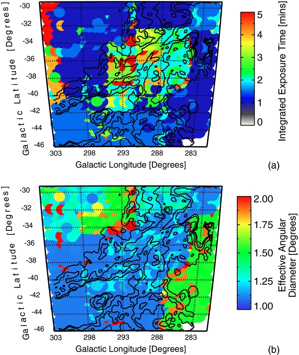
Figure 2. Total integrated exposure time (a) and smoothed angular diameter of each sight line (b) of survey. The total integrated exposure time consists of multiple 30 s individual observations at each location of the Hα Magellanic Bridge survey. Each observation spans 200 km s−1, which is only part of the 0 to +315 km s−1 velocity coverage. The majority of the observations were centered at either +175 or +210 km s−1. The smoothed angular diameter is the effective diameter of the sight line after binning the non-Nyquist sampled observations such that they conform to the Nyquist grid spacing. The contours depict the 1019 cm−2 H i column density at 10, 20, 35, and 50 increments.
Download figure:
Standard image High-resolution imageThe observations taken with different spacing from the Nyquist grid were binned to conform to the Nyquist grid. This corresponds to 28% of the resultant average sight lines having a smoothed angular coverage with an effective angular diameter of 11 or less, 55% with 12 or less, and 92% with 20 or less compared to the 1° angular resolution of WHAM. We define the effective angular diameter as the diameter of a circle with an area equal to the total area covered by the averaged beams. The farther from the main H i structure of the Bridge, the larger the average displacement of the non-Nyquist sampled observations from the Nyquist grid points as these locations were sampled fewer times. The typical effective angular diameter is therefore smallest along the H i Bridge, as illustrated in Figure 2(b).
3. DATA REDUCTION
Beyond the ring-summing and flat-fielding procedures described in Haffner et al. (2003), the data reduction of the Hα map included velocity calibration of the emission, subtraction of the atmospheric emission, stitching together of the spectra taken along the same sight line taken at different velocity intervals, and applying an extinction correction to the Hα emission from both foreground dust and dust within the Bridge.
3.1. Velocity Calibration
Once the spectra are pre-processed, ring-summed, and flat-fielded, they are in 2 km s−1 bins over a 200 km s−1 velocity window. These spectra are shifted to the geocentric (geo) velocity frame by adding a constant velocity offset value, determined by identifying bright atmospheric lines with known wavelengths. Both faint and bright atmospheric emission clutter the −50 to +315 km s−1 LSR velocity window of this Hα Magellanic Bridge survey. Two bright atmospheric lines dominate the spectra in this survey: the bright geocoronal line at vgeo = −2.3 km s−1 and a bright OH line at vgeo = +272.44 km s−1 relative to the Hα recombination line at 6562.8 Å. These two bright lines are labeled (i) and (ii) in Figure 3(a). Because the velocity window of a single observation is only 200 km s−1 wide, multiple exposures are needed to fully sample the spectrum of the Bridge. Each exposure was shifted to include either the geocoronal line or the bright OH line to enable accurate velocity calibration. Although the overlapping emission from the Galactic warm interstellar medium (ISM)—marked as (iii) and (iv) in Figure 3(b)—with the geocoronal line can add uncertainty in determining positions of emission features below +50 km s−1, the large contrast in the strengths of these lines generally makes locating the geocoronal-line center easy. Finally, we apply an offset for each observation that shifts them to the LSR frame.

Figure 3. Average Hα emission toward (l, b) = (600, −670) and (890, −710). Panels (a) and (b) show this average spectra as a dotted line and the corresponding fit in gray. Panel (b) emphasizes the faint emission in panel (a) and displays the constructed atmospheric template as a black solid line. Panel (c) illustrates the faint atmospheric lines near Hα in dark gray against the fit for the averaged spectra; these faint lines are listed according to the line identification in Table 1. At +334.4 km s−1, an additional line—not shown here—with an FWHM of 15.0 km s−1 and 2.76 times the area of line (1), was added to the construction of the average atmospheric template. Panel (d) displays the residuals between the average spectra and the total fit. The (i) marker indicates the geocoronal line at −2.3 km s−1 and the (ii) marker denotes a bright OH line at a geocentric velocity of +272.44 km s−1. Galactic emission is labeled by markers (iii) and (iv). Marker (v) indicates residuals from the OH line subtraction caused by a slight mismatch in instrument profile; we decreased these residuals in the final data processing by applying a custom instrument profile for each night (see Section 3.2.2).
Download figure:
Standard image High-resolution image3.2. Removing Atmospheric Emission
The overlap of the geocoronal line with the Hα Magellanic Bridge emission is negligible as the majority of low-velocity H i components appear at vgeo > +30 km s−1. The bright OH line contaminates the spectra at +260 km s−1 ≲ vgeo ≲ +290 km s−1. As a result, this line does occasionally overlap with the Hα emission features close to LMC velocities. Fainter atmospheric emission is present below ∼0.1 R at all velocities in this survey. The removal of both the bright and faint atmospheric lines is crucial for detecting the faint Hα emission between the Magellanic Clouds. The removal of atmospheric contamination consists of three steps: subtracting the background continuum, subtracting the bright atmospheric lines, and subtracting the faint atmospheric lines.
3.2.1. Background Subtraction
We assume an underlying flat background continuum level over all velocities. The baselines are well behaved over the velocity range of this survey, except when contaminated by emission from bright foreground stars. Foreground stars distort the shape of the spectra and create an elevated, nonlinear background with absorption lines. Beams that contain stars with mV < 6 (∼ 9%) within a 055 radius are excluded from this survey to minimize this foreground contamination and are replaced with an average of the uncontaminated observations within 1°.
3.2.2. Bright Atmospheric-line Subtraction
The strength of the bright and faint atmospheric lines vary differently throughout the course of a night and a year. The geocoronal line (Mierkiewicz et al. 2006) and OH lines (Meriwether 1989) are produced from interactions between solar radiation and Earth's upper atmosphere and will, therefore, vary in strength with the direction and the time of the observation. These bright atmospheric lines are displayed in Figure 3(a) and are labeled (i) and (ii). For this reason, the geocoronal line and the OH line at vgeo = +272.44 km s−1 are always individually removed from each spectra before subtracting the faint atmospheric lines. We removed these lines by fitting a single Gaussian profile convolved with the instrument profile.
Two effects alter the shape of bright atmospheric lines. (1) The precision in aligning the dual-etalon transmission functions (spectrometer "tuning") can result in very slight night-to-night variations in the instrument profile at a level only detectable in narrow, bright lines. (2) A geocoronal "ghost"—due to an incomplete suppression of a geocoronal line at vgeo = −2.3 km s−1 from a neighboring order in the high-resolution etalon (see Haffner et al. 2003, Figure 2)—lies underneath the OH line at vgeo = +272.44 km s−1. Although these effects are minimal, together they can leave residuals that can make detecting the faint Hα emission of the diffuse Magellanic Bridge difficult. Each night we constructed a new instrument profile to minimize the residuals associated with the subtraction of the geocoronal and OH lines to account for both of these effects. The P Cygni shape of the residual in Figure 3(d), marked (v), illustrates the result of the line subtraction with the generic WHAM instrument profile instead of using a custom instrument profile each night.
We constructed the instrument profile for each night by modeling the shape of the +272.44 km s−1 OH line with three Gaussians: one to account for the global size and width of the line and one for each wing to account for an asymmetrical shape of the line at the blue wing. The asymmetrical blue wing is due to minor etalon defects (Tufte 1997). We chose to model the instrument profile using the OH line because its intrinsic line width is much narrower than the instrument width and because it is well separated from Galactic emission. We created these profiles from observations toward either (l, b) = (600, −670) or (890, −710), two sight lines that are observed to have little Hα emission and are located far outside of the  to (3025, −467) Bridge survey.
Due to the high signal strength of the OH line and the subsequent increased noise, the data that overlap with OH line are more noisy than the surrounding spectra. The net result is that the sensitivity of our survey is better at lower velocities between +100 km s−1 ⩽ vLSR ⩽ +240 km s−1 with IHα ≃ 30 mR than at higher velocities between +240 km s−1 ⩽ vLSR ⩽ +275 km s−1 with IHα ≃ 40 mR.
Bridge emission at high velocities may be reduced over certain velocities since the some of the emission could be subtracted during the removal of the bright OH line. The intensity of the OH line dominates over this span, hiding Hα emission from the Bridge. Removal of some Bridge emission is unavoidable throughout the core of this line. The presence of ionized gas emission over this narrow velocity range may be revealed through other spectral lines, such as [S ii] or [N ii]. We are undertaking Magellanic Bridge surveys in these lines as well with WHAM.
In the wings of the OH line, the atmospheric and potential Bridge emission become comparable. As mentioned above, determining the instrument profile each night helps to minimize any residuals from subtracting the line. We also observe each sight line multiple times over multiple months so the offset between the geocentric and LSR frames is different for each observation. Combining these multiple-epoch observations minimizes contamination from the OH wing in an individual exposure.
3.2.3. Faint Atmospheric-line Subtraction
In addition to the bright geocoronal and an OH atmospheric line, faint atmospheric lines litter the spectra. The strength of these faint atmospheric lines changes primarily with airmass. To characterize them, we observed two directions faint in Hα emission multiple times over 10 days to create an average spectrum with a high signal-to-noise ratio. This averaged spectrum consists of numerous 30 and 60 s observations, totaling 4.5 hr of integrated exposure time, toward (l, b) = (600, −670) and (890, −710), which are outside the Bridge survey region of  to (3025, −467). Table 1 lists the geocentric velocity, wavelength, width, and relative intensity of these atmospheric lines and Figure 3(c) displays their relative size and position. Hausen et al. (2002) and Haffner et al. (2003) list similar characteristics for the faint atmospheric lines near Hα in the northern hemisphere observed toward the Lockman Window; however, our observations here extend this list to higher positive velocities. We used the averaged atmospheric emission spectrum of the faint lines to construct a synthetic atmospheric template (shown in Figure 3(b) as a solid black line).
Table 1. Faint Atmospheric Lines Near Hα
| Line | vgeo | Wavelength | FWHM | Relative |
|---|---|---|---|---|
| (km s−1) | (Å) | (km s−1) | Intensity | |
| 1 | −41.4 | 6561.92 | 10 | 1.00 |
| 2 | −24.9 | 6562.29 | 10 | 0.30 |
| 3 | +32.7 | 6563.57 | 10 | 0.30 |
| 4 | +40.9 | 6563.75 | 10 | 0.65 |
| 5 | +54.2 | 6564.04 | 10 | 0.39 |
| 6 | +73.0 | 6564.46 | 15 | 1.60 |
| 7 | +96.5 | 6564.98 | 10 | 0.36 |
| 8 | +140.4 | 6565.95 | 15 | 0.90 |
| 9 | +174.7 | 6566.71 | 15 | 2.36 |
| 10 | +201.4 | 6567.31 | 15 | 1.69 |
| 11 | +218.8 | 6567.69 | 15 | 1.13 |
| 12 | +236.8 | 6568.09 | 10 | 1.34 |
| 13 | +255.5 | 6568.51 | 15 | 1.84 |
| 14 | +292.6 | 6569.33 | 10 | 0.92 |
| 15 | +311.5. | 6569.75 | 15 | 1.06 |
Note. This list excludes the geocoronal line at −2.3 km s−1 and the bright OH line at +272.44 km s−1: two lines produced through a different process in a different atmosphere layer.
Download table as: ASCIITypeset image
We removed the faint atmospheric lines from the Magellanic Bridge observations by scaling the synthetic atmospheric template—which accounts for changes in the flux due to airmass and daily fluctuations—to match the atmospheric contamination. This scaled atmospheric template is then subtracted from the observation. The removal of the faint atmospheric lines in this study parallels the reduction method used by Haffner et al. (2003), which provides a more thorough description of this process. Figure 4 illustrates this process toward (l, b) = (890, −710), a sight line far off the Magellanic Bridge and faint in Hα emission, and toward (l, b) = (2894, −390), a sight line in the middle of the Magellanic Bridge. Both of these observations were taken on the same night. Panels (b.1) and (b.2) show the scaled atmospheric template (solid gray line) fit to these spectra and the resultant atmospheric-subtracted spectra in panels (c.1) and (c.2); the bright OH—centered roughly at +250 km s−1 in the LSR frame—and the background continuum were fit and subtracted separately.
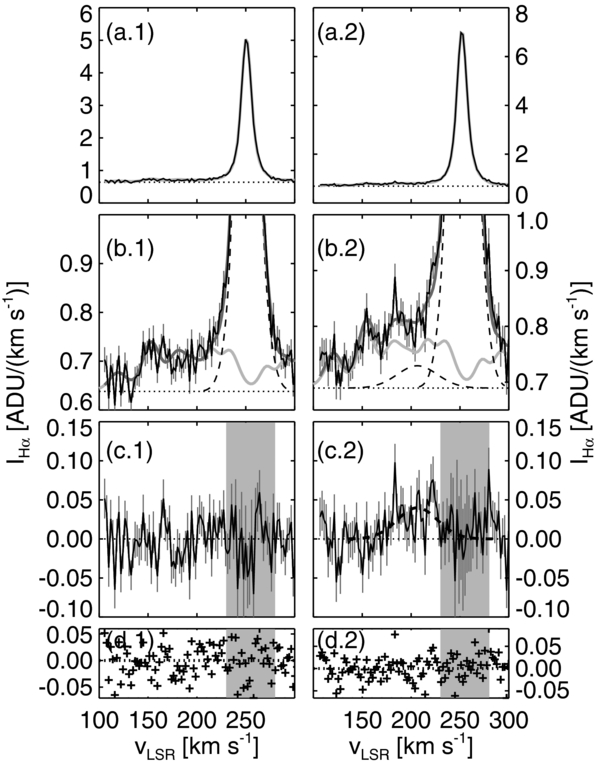
Figure 4. Example of atmospheric subtraction. Panels (a.1)–(d.1) correspond to an observation taken toward (l, b) = (890, −710), one of the faint directions used to construct the atmospheric template in Figure 3. Panels (a.2)–(d.2) correspond to an observation taken toward the inner region of the Bridge at (l, b) = (2894, −390) with a non-extinction-corrected IHα of 0.08 R. The pre-atmospheric spectra are shown in panels (a.1) and (a.2) and zoomed-in to illustrate the faint emission in (b.1) and (b.2). The dotted lines in panels (a.1)–(b.2) indicate the location of the baseline. The dashed lines in panels (b.1) and (b.2) trace the bright OH line at a geocentric velocity of +272.44 km s−1 and an Hα emission feature produced from the Magellanic Bridge in panel (b.2). The fainter, solid, gray line in panels (b.1) and (b.2) indicate the strength and location of the faint atmospheric lines, identified using the atmospheric template in Figure 3. The darker, solid, gray line in panels (b.1) and (b.2) indicate the total fit, which includes the baseline, atmospheric template, and contributions from the OH and Hα Bridge emission lines. Panels (c.1) and (c.2) include the spectra after subtracting the atmospheric profile, the bright OH line, and the baseline. The residuals of the fit are displayed in panels (d.1) and (d.2). The region highlighted in gray in panels (c.1) and (c.2) represent the location where a bright OH line was removed and signifies a velocity range with a lower sensitivity than the surrounding spectra.
Download figure:
Standard image High-resolution image3.3. Co-adding Spectra
Each observation produces an average spectrum of the emission within the 1° beam over a 200 km s−1 wide velocity window at a velocity resolution of 12 km s−1. The dominant H i emission of the Magellanic Bridge spans approximately +50 to +315 km s−1. With this wide velocity range—one and a half the size of the WHAM velocity window—we covered the spectral range with multiple exposures and spliced them together. The spectra were first velocity calibrated and atmospheric subtracted by the methods described in Sections 3.1 and 3.2, then combined. Figure 5 shows an example of how we combined five separate observations along the same sight line after velocity calibration and atmospheric subtraction. The resultant spectrum in Figure 5(c) is an average of the five multi-color spectra shown in Figure 5(b), with the intensity and uncertainty weighted by the number of observations at each velocity bin. We selected the velocity coverage for each observation to ensure the inclusion of a bright atmospheric line with a stationary position in the geocentric rest frame to ensure accurate alignment.
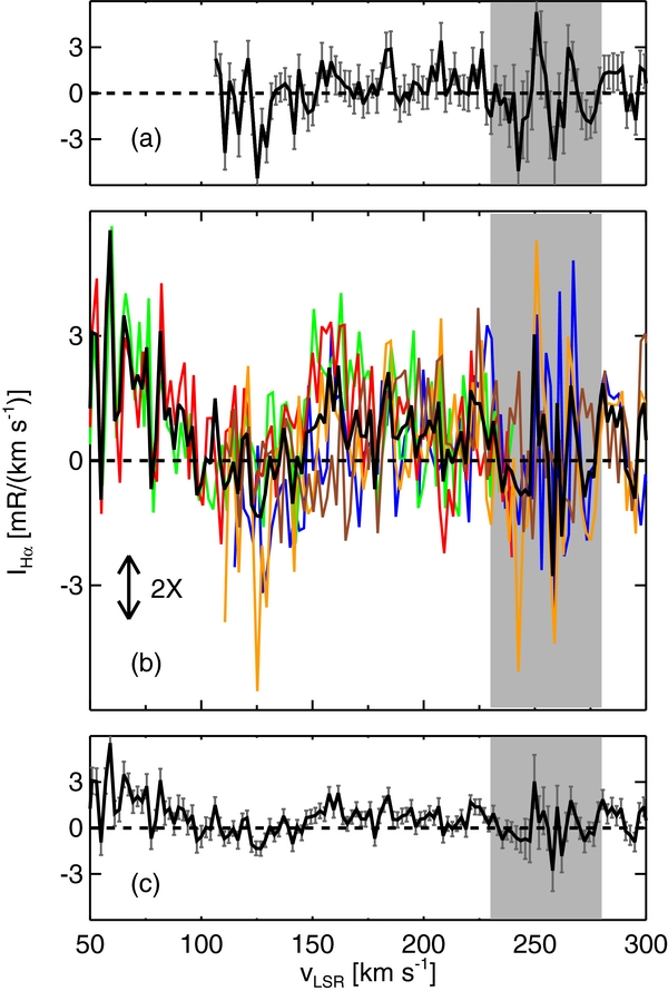
Figure 5. Combining spectra taken over three months toward the direction (l, b) = (2916, −390). Panel (a) shows an example of a typical observation and the corresponding error. Panel (b) displays five separate observations, each illustrated with a different color, and their combined average (black) with the y-axis expanded by a factor of two. This average spectra is displayed again in panel (c) with the resulting errors. The elevated intensity between +50 and +100 km s−1 is due to Galactic emission; for this reason, velocities below +100 km s−1 are excluded from the Hα map in Figure 7. The region highlighted in gray represent the location where a bright OH line was removed; our sensitivity is lower throughout this velocity region.
Download figure:
Standard image High-resolution imageIn Figure 6, we demonstrate the entire reduction process toward sight line at  in the Magellanic Bridge with two separate observations. The reduced combined spectrum is shown in panel (a). Panels (b.1) and (b.2) include the non-reduced spectra and panels (c.1) and (c.2) zoom in on the faint atmospheric lines and Bridge emission with their corresponding fits. We measure similar Bridge emission from both of these observations before and after we splice the two spectra together.

Figure 6. Reduction of sight line  in the Magellanic Bridge with two separate observations (obs 1 and obs 2). Panel (a) shows the fully reduced spectra with horizontal arrows and vertical dotted lines labeling the +100 to +300 km s−1 velocity range of the Hα survey. This sight line has a non-extinction-corrected IHα of 0.18 R. The unreduced spectra in panels (b.1) and (b.2) are magnified in (c.1) and (c.2) to highlight the faint atmospheric lines and Bridge emission of the non-reduced spectra, where a solid gray line marks the total fit, a hollow gray line signifies the atmospheric template of the faint lines, the outlined gray dashed line labels the bright OH line fit at vgeo = +272.44 km s−1, and the gray dashed line traces the Bridge emission. The residuals of the emission from these two observations minus the total fits are included in panels (d.1) and (d.2). The region highlighted in gray represents the location of a bright OH line and signifies a velocity range with a lower sensitivity than the surrounding spectra.
Download figure:
Standard image High-resolution image3.4. Hα Extinction Correction
The intrinsic Hα intensity from the Magellanic Bridge is reduced by foreground dust in the MW and potentially by the dust within the structure itself. In this section, we discuss our prescription for determining the extinction correction due to these sources.
3.4.1. Correction for Foreground ISM Extinction
The position of the Magellanic Bridge below the Galactic plane results in minimal foreground interstellar dust extinction. We expect that most of the extinction comes from local interstellar dust. We use the excess color given in Diplas & Savage (1994) for a warm diffuse medium:

where the average H i column density (〈NH i〉) includes only the foreground H i emission (Bohlin et al. 1978). The integrated foreground H i column density is calculated from smoothed Leiden/Argentine/Bonn Galactic H i survey (LAB; Kalberla et al. 2005; Hartmann & Burton 1997) data to match our 1° angular resolution. To calculate the total foreground extinction along the line of sight, we integrated H i column densities over the −450 to +100 km s−1 LSR velocity range. If the extinction follows the 〈A(Hα)/A(V)〉 = 0.909 − 0.282/Rv optical curve presented in Cardelli et al. (1989) for a diffuse ISM, where Rv ≡ A(V)/E(B − V) = 3.1, then the expression for the total extinction becomes

so that the foreground extinction correction is IHα, corr = IHα, obse A(Hα)/2.5. All subsequent mass and ionizing flux calculations are corrected for foreground extinction using the LAB survey H i column densities, unless otherwise specified.
3.4.2. Correction for Magellanic Bridge ISM Extinction
H i emission traces most of the dust responsible for the extinction in the inner region of the Bridge. FUSE observations toward the early-type star DI-1388 at (2912, −413) reveal only  (Lehner 2002) and no H2 absorption toward the early-type star DGIK-975 at (2872, −361), which indicates that the faction of H2 of the diffuse gas in the central regions of the Bridge is less than 0.004% (Lehner et al. 2008). The non-detections of 12CO(1–0) by Smoker et al. (2000) indicates that this region only contains trace amounts of molecular gas. The lack of molecular gas detections suggests that this region also contains only trace amounts of dust. Therefore, we did not apply an extinction correction the central region of the Bridge, which would have only increased the Hα intensity by a maximum of 1.5% (see Table 2), assuming that this region has a composition similar to the SMC-Tail.
Table 2. Neutral and Ionized Properties
| Region | Foreground Extinction | Internal Extinction | ||||
|---|---|---|---|---|---|---|
| log 〈NH i〉 | A(Hα)a | %corra | log 〈NH i〉 | A(Hα)a | %corra | |
| (cm−2) | (mag) | (cm−2) | (mag) | |||
| Inner regionb | 20.8 | 0.26 | 27.3% | 19.9 | 0.02 | 1.5% |
| H i SMC-Tailb | 20.6 | 0.17 | 16.7% | 20.5 | 0.07 | 6.8% |
| Hα SMC-Tailb | 20.6 | 0.16 | 15.6% | 20.4 | 0.05 | 5.2% |
Notes.
aCalculated using the average log 〈NH i〉 of the region.
bRegions defined by a polygon with the following corners: l = (2890, 2830, 2890, 2970) and b = (− 302, −380, −430, −350) for the inner region, l = (3018, 2959, 2891, 2957) and b = (− 394, −362, −430, −465) for the H i SMC-Tail, and l = (3005, 2945, 2920, 2970) and b = (− 410, −395, −420, −450) for the Hα SMC-Tail. The boundaries for these regions are displayed in Figure 1.
Download table as: ASCIITypeset image
The composition of the SMC-Tail is different than the central regions of the Magellanic Bridge, where dust and molecular gas have been directly observed (see Mizuno et al. 2006; Gordon et al. 2009). Gordon et al. (2003) determined the extinction properties of the SMC-Wing by measuring stellar reddening. They found that E(B − V) = 0.263 mag, RV ≃ 2.05, and  . To determine the Hα extinction in the SMC-Tail, we use the extinction curve presented in their study:
  , where E(Hα − V) = 0.277 mag (Gordon et al. 2003; Equations (1) and (4)). This yields the extinction correction for the Hα emission of the SMC-Tail:

We apply this extinction correction to only the SMC-Tail region, where 〈NH i〉 is determined using the results from the LAB H i survey smoothed to 1° to match our angular resolution. Correcting the Hα intensities for the dust within the structure results in an average 5.2% increase for the Hα SMC-Tail and 6.8% for the H i SMC-Tail (see Table 2 and Figure 1) with H i column densities integrated over the +100 to +300 km s−1 in the LSR velocity range. Because the Hα emitting regions lie throughout the SMC-Tail and not behind the structure, this extinction correction represents an upper limit for the Hα intensities correction.
4. Hα INTENSITY MAP
We surveyed the Magellanic Bridge and SMC-Tail in Hα with WHAM from  to (3025, −467) over a velocity range of 0 to +315 km s−1 in the LSR frame. Figure 7 displays both the non-extinction-corrected Hα intensity and the H i column density over this region, integrated over +100 km s−1 ≲ vLSR ≲ +300 km s−1. We used Galactic All Sky Survey (GASS) for all the H i spectra, the H i maps, and the H i calculations in this paper (McClure-Griffiths et al. 2009; Kalberla et al. 2010)—except when calculating the extinction correction in Section 3.4 where we used the LAB survey—smoothed to 1° to match the angular resolution of the WHAM observations. To avoid contamination from the Galactic warm ISM, we exclude emission with velocities less than +100 km s−1. At LSR velocities greater than +300 km s−1, emission from the LMC contributes in low-longitude and high-latitude regions of the map; for this reason, we chose to also exclude emission at velocities greater than +300 km s−1. As mentioned in Section 3.2.2, the sensitivity of this survey is decreased from IHα ≃ 30 mR to IHα ≃ 40 mR at vLSR ∼ +250 km s−1 due to residuals in the bright OH line subtraction at vgeo = +272.44 km s−1.
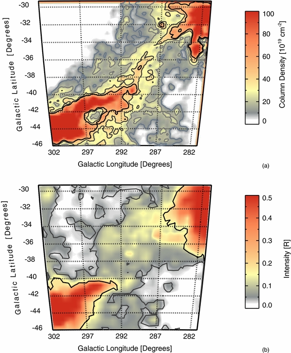
Figure 7. (a) H i and (b) Hα emission maps from the GASS survey and WHAM observations, respectively. The emission is integrated over the vLSR range of +100 to +300 km s−1. The contour lines in panel (a) trace the 1019 cm−2 H i column density at increments of 10, 20, 35, and 50. The contour lines in panel (b) trace the non-extinction-corrected Hα intensity at 0.03 and 0.16 R. The brightest Hα emission follows the high column density H i gas in the Small Magellanic Cloud Tail (lower left) and the Large Magellanic Cloud (upper right).
Download figure:
Standard image High-resolution imageHα emission, with typical intensities above 0.1 R, spans the entire Magellanic Bridge and SMC-Tail roughly tracking the H i emission. Portions of the Hα Bridge exist at slightly higher latitude than the bright H i Bridge, e.g., the patches of Hα emission at (297°, −34°) and (295°, −32°) in Figure 7(b). Fainter H i emission at column densities of 1018 cm−2 does span to these higher latitudes, suggesting that this region could be highly ionized. In Figure 7, near the LMC and in the region between  and (283°, −45°), the average H i emission has a higher mean velocity where our measured Hα intensity is low. The loss in Hα sensitivity due to the OH line at higher velocities could lead to under representation of emission in certain spatial regions. The general spectroscopic agreement between H i and Hα throughout the Bridge combined with our decreased sensitivity limit of IHα ≃ 40 mR over +240 km s−1 ⩽ vLSR ⩽ +275 km s−1 does not preclude the existence of diffuse ionized gas with low emission levels associated with the neutral component. Emission maps in other spectral lines (e.g., [S ii] or [N ii]) may help reveal undetected gas in these regions.
The Hα emission decreases radially with distance from both of the Magellanic Clouds past the 0.16 R contour. The emission becomes constant in the central 10° of the Bridge, past the 0.16 R contour, where the non-extinction-corrected intensity ranges from 0.05 R ⩽ IHα ⩽ 0.16 R. The SMC H i-Tail extends further than the Hα-Tail by a few degrees, where intensities are typically less than 0.4 R.
An elevated region of Hα emission exists within the Magellanic Bridge at  , just off the bright NH i = 5 × 1020 cm−2 contour of the H i SMC-Tail as displayed in Figure 7. A bright foreground star, with MV = 4.7 mag at
  , aligns with this line of sight. Although we replaced the spectra of the Hα map with the average of the nearby spectra for the sight lines within a radius of 10 of the star, this region is still brighter than the neighboring sight lines. The profile of the resultant Hα spectra in this region agree with the H i spectra, with H i emission features at +150 km s−1 ⩽ vLSR ⩽ +200 km s−1 and Hα features at +150 km s−1 ⩽ vLSR ⩽ +250 km s−1, where the H i column density peaks at +180 km s−1 compared to +170 km s−1 for the Hα. The Hα spectra also have a less prominent component at +225 km s−1. The emission feature is only present in the neighboring H i spectra at more negative latitudes. The similarities between the Hα and H i spectral components suggest that this rise in Hα intensity at this location is real.
Although large-scale structure of the Hα and H i Bridge agree, there are subtle differences at small scales. In the region above the main bridge, with more positive latitudes, there are small patches of elevated Hα emission at roughly  , and (2880, −450). The elevation in Hα could be explained if these regions are correlated with star-forming sites, are more exposed to the Lyman continuum of the LMC and SMC, or are indicators of shock-heated gas that is produced as the Magellanic Bridge travels through MW halo gas.
An elongated, faint Hα feature exists off the Hα Bridge that spans a minimum 10° from  and
and  that might be material associated with the Leading Arm or stellar outflows from the SMC. This structure is at the edge of our Hα Bridge survey and may extend to higher Galactic longitudes and latitudes. The Hα emission component of this structure ranges from +140 km s−1 ⩽ vLSR ⩽ +210 km s−1, with typical intensities of roughly 0.03 R. The lack of a complementary H i emission above NH i = 1.6 × 1018 cm−2, the 3σ sensitivity of the GASS H i survey at a width of 30 km s−1 (McClure-Griffiths et al. 2009), combined with the faint Hα emission could indicate that this gas is low-density or hot (T > 105 K) medium. Although this structure is very faint, it is likely real as the velocity components persist throughout the structure. Figure 8 shows the H i and Hα spectra at three locations along this structure. These velocity components are at velocities similar to those observed in the SMC. The small angular distance and velocity difference suggests that this gas is associated with the SMC. With the high star formation rate of the SMC and the galaxy interactions with the LMC and MW, this structure is probably associated with either SMC stellar feedback or displaced material, removed by galaxy interactions.
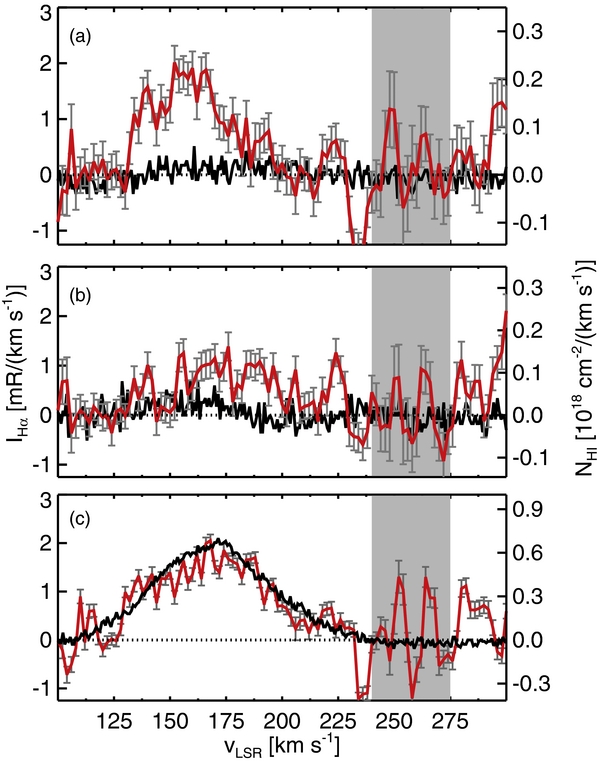
Figure 8. Comparison of non-extinction-corrected Hα intensity (red) and H i column density (black) associated with an elongated, faint Hα feature that extends off the Hα Bridge and spans from  to (302°, −30°). Panel (a) includes the emission at (3020, −307), panel (b) at (3019, −351), and panel (c) at (3018, −401). The region highlighted in gray represents the location where the bright OH line was removed, marked as (ii) in panel (a) of Figure 3 and represents a region where our sensitivity is low.
Download figure:
Standard image High-resolution image5. COMPARISON OF THE Hα AND H i GAS
The large- and small-scale similarities and differences between the neutral and ionized gas phases provide clues to the processes affecting the structure. In this section, we compare the differences between the H i and Hα velocity distribution and the strength of these emission lines.
5.1. H i and Hα Velocity Distribution
The Magellanic Bridge has a complex velocity distribution. The first moment (also known as the intensity-weighted mean velocity or velocity field:  ) of the Hα increases from roughly +175 to +225 km s−1 across the Magellanic Bridge from the SMC-Tail to the LMC. The H i increases from roughly +125 to +250 km s−1 over the same region. These global velocity trends are shown in Figure 9. The smooth Hα and H i velocity gradients are a result of blending multiple components in constructing the first moment map. Brüns et al. (2005) suggest that the H i velocity gradient is largely due to projection effects and indicates that the Magellanic Bridge is likely orbiting parallel with the Magellanic Clouds.
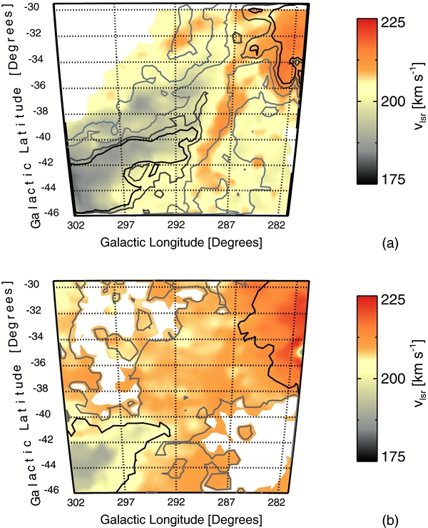
Figure 9. (a) H i and (b) Hα first moment map for the H i column densities greater than 1020 cm−2 and the Hα intensities greater than the 0.03 R. The contour lines in panel (a) trace the 1019 cm−2 H i column density at increments of 10, 20, 35, and 50. The contour lines in panel (b) trace the non-extinction-corrected Hα emission at 0.3 and 0.16 R.
Download figure:
Standard image High-resolution imageThe Hα first-moment map has a much smoother distribution than the corresponding H i map. Three effects cause this difference. (1) The Hα emission is much broader than the H i, both in the width of the individual components and in the overall velocity extent of the multiple components. (2) The angular resolution of the Hα survey is much lower than the H i GASS survey at 1° compared to 16'. Each Hα observations spans a spatial diameter of ∼1 kpc, assuming a distance of 55 kpc, which causes all the small-scale structure to be blended together and diluted in the resultant spectra. (3) The Hα survey is less sensitive over the velocity range of +240 km s−1 ⩽ vLSR ⩽ +275 km s−1 due to the residuals from a bight atmospheric OH line (see Section 3.2.2); the average emission of the Bridge shifts to vLSR ≳ +240 km s−1 at the sight lines closest to the LMC, causing the Hα first map to be less accurate for the faint emission in this region.
Although the global velocity distribution of the H i and Hα gradually shifts from the SMC to the LMC, the individual spectra have a complex multi-component structure that often has two or more components (see Figures 10 and 12). The majority of the brightest H i and Hα components peak at roughly the same velocity at most locations; however, there are many places where the dominant Hα peak corresponds to a weaker H i peak. This behavior is especially true in the SMC-Tail and near the LMC. Such regions may have a higher ionization fraction, which could indicate active local star formation, more exposure of the gas to ionizing radiation from the galaxies, or an interface between the neutral and ionized gas.
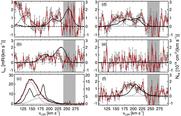
Figure 10. Comparison of non-extinction-corrected Hα intensity (red) and H i column density (black) across the Magellanic Bridge. The dotted Gaussians trace individual Hα components; the dashed line is the sum of these components. The region highlighted in gray represents the location where the bright OH line was removed, marked (ii) in panel (a) of Figure 3 and represents a region where our sensitivity is low. Emission from the SMC-Tail is shown in the three left panels: (a) at (2908, −440), (b) at (2932, −460), and (c) at (2975, −425). Panel (d) at (2945, −360) displays typical emission features toward the middle of the Magellanic Bridge and panel (e) at (2962, −334) illustrates a typical observation off the Hα Bridge; this flat spectrum indicates that the atmospheric emission has been adequately removed. Panel (f) at (2895, −328) shows representative spectra at the Magellanic Bridge and LMC interface.
Download figure:
Standard image High-resolution imageA statistical investigation of the H i gas components in the SMC-Tail using the Australia Telescope Compact Array and the Parkes telescopes indicates that the multi-component structure might be associated with two kinematically and morphologically distinct arms of gas emanating from the SMC (Muller et al. 2004). Numerical simulations by Gardiner et al. (1994) predict that the lower velocity and more southern arm would extend to the LMC. Figure 10 includes a comparison of typical H i and Hα spectra toward three locations in the SMC-Tail where the neutral gas exhibits this multi-peaked distribution. In Figure 10(a), the bright H i emission aligns with the Hα emission, but in Figures 10(b) and (c) the peak in Hα traces the faint H i peak. Many of the Hα sight lines toward the SMC-Tail have a two component Hα velocity distribution, including the spectrum shown in Figure 10(c).
In the Magellanic Bridge, the Hα emission has velocity components that lack complementary H i component, possibly revealing a highly ionized region. An example of this behavior is shown in Figure 10(d) toward (l, b) = (2945, −360) at vLSR ∼ 165 km s−1. Figures 11(a.1)–(a.3) show a mini map of the H i emission used to produce the spectra in Figure 10(d), with the 1° averaged region outlined in black. The velocity range of Figure 11(a.2) channel map was chosen to highlight the emission where the smoothed H i spectral components differ from the Hα components. The small-scale structure of the H i gas enclosed within the same angular extent as the WHAM observations reveals a small subregion with a complementary component at +165 km s−1 toward (2943, −365) with NH i ∼ 5 × 1019 cm2.
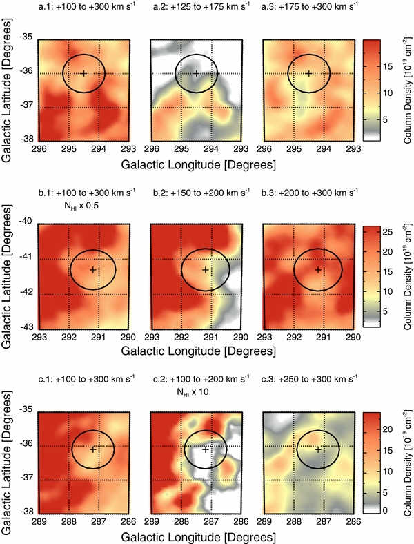
Figure 11. H i column density sub-maps illustrating the substructure of the neutral gas within one WHAM beam. The emission along these three sight lines produces Hα and H i spectra that differ in component structure when the H i is smoothed to the same angular resolution. Panels (a.1)–(a.3) include the H i Bridge emission at (2945, −360) (see Figure 10(d)), panels (b.1)–(b.3) include emission toward early-type star DI 1388 at (2912, −413) (see Figure 12(a)), and panels (c.1)–(c.3) include emission toward early-type star DGIK 975 at (2872, −361) (see Figure 12(b)). Panels (a.1)–(c.1) integrate the emission vLSR from +100 to +300 km s−1, panel (a.1) from +100 to +175 km s−1, (b.1)–(c.2) from +100 to +200 km s−1, (a.3) from +175 to +300 km s−1, and (b.1)–(c.3) from +200 to +300 km s−1. The regions used to produce these spectra are outlined within the large black circles, depicting the WHAM beam size.
Download figure:
Standard image High-resolution imageLehner et al. (2008) also identified highly ionized regions in the inner region of the Magellanic Bridge from the absorption in the spectra of two early-type stars: DI 1388 at (l, b) = (2912, −413) and DGIK 975 at (l, b) = (2872, −361) marked in Figure 12; FUSE observations from that study revealed gas that is mostly ionized at +165 km s−1 ⩽ vLSR ⩽ +193 km s−1 and partially ionized at +193 km s−1 ⩽ vLSR ⩽ +215 km s−1 toward DI 1388 and that the gas at +140 km s−1 has a higher ionization fraction than the gas at +175 km s−1 toward the DGIK 975 sight line. The Hα and H i spectra toward these two early-type stars are displayed in Figure 12 where the center of the H i components are marked with green and the positions of the UV-absorption features are marked with purple. The lack correlation of the UV absorption with the Hα and H i emission at +140 km s−1 in the DGIK 975 sight line suggests this component is highly ionized and possibly influenced by a different process or is exposed to more ionizing flux than the gas at +175 km s−1, which aligns with a bright Hα emission line.
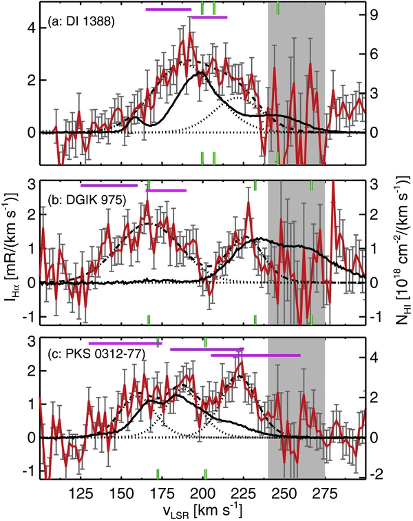
Figure 12. Comparison of non-extinction-corrected Hα intensity (red), H i column density (black), and UV-absorption species. The dotted Gaussians trace individual Hα components; the dashed line is the sum of these components. The green markings indicate the center position of H i emission features and the purple markings indicate the location of known absorption features. The region highlighted in gray represents the location where the bright OH line was removed, marked as (ii) in panel (a) of Figure 3; unfortunately, this study is insensitive to faint Hα emission in this gray region as this emission could easily be subtracted during the OH line removal. Emission toward the early-type star DI 1388 is shown in panel (a) at (2912, −413), early-type star DGIK 975 in panel (b) at (2872, −361), and toward background quasar PKS 0312-77 in panel (c) at (2935, −374). Lehner et al. (2008) found that the sight line DI 1388 is mostly ionized at +165 km s−1 ⩽ vLSR ⩽ +193 km s−1 and partially ionized at +193 km s−1 ⩽ vLSR ⩽ +215 km s−1. Sight line DGIK 975 has two absorption features at +140, +175 km s−1, where the higher velocity component is more neutral; both of these sight lines are toward early-type stars. The PKS 0312-77 sight line, toward a background quasar and shown in panel (c), has absorption features at +160, +200, +240, and +310 km s−1 (N. Lehner 2011, private communication).
Download figure:
Standard image High-resolution imageBoth the DI 1388 and DGIK 975 sight lines have Hα emission below +200 km s−1 that is absent in the averaged H i spectra in Figures 12(a) and (b). Figures 11(b.1)–(b.3) and (c.1)–(c.3) include mini H i emission maps of the region used to produce these H i spectra. Both of the low-channel maps contain subregions with bright H i emission within the averaged 1° region that become dilute when averaged with the surrounding faint emission. These figures illustrate that—although the Hα observations excel at mapping the large-scale structure of this diffuse Bridge—the small-scale details of the ionized gas are unresolvable and might vary greatly within one WHAM beam as seen in the H i.
5.2. Hα Intensity and H i Column Density
The global morphology of the Hα and H i emission agree (see Figure 7). The regions near the Magellanic Clouds behave similarly in H i and Hα. Between the galaxies, both the Hα intensity and H i column densities decrease substantially. Figure 13(a) compares the H i column density and non-extinction-corrected Hα intensity for each sight line in the entire region of this survey over +100 km s−1 ⩽ vLSR ⩽ +300 km s−1. The gray dashed lines and the corresponding gray, open diamonds mark where measurements fall below the sensitivity of WHAM or the GASS H i survey. The sensitivity of our survey is IHα ≃ 30 mR between +100 km s−1 ⩽ vLSR ⩽ +240 km s−1 but rises to IHα ≃ 40 mR between +240 km s−1 ⩽ vLSR ⩽ +275 km s−1 due to the increased noise from the subtraction of the bright OH line at vgeo = +272.44 km s−1. The sensitivity of the GASS H i survey is NH i = 1.6 × 1018 cm−2 at a width of 30 km s−1 (McClure-Griffiths et al. 2009).
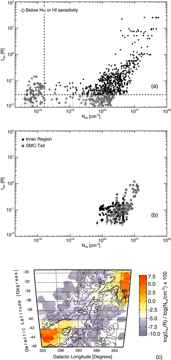
Figure 13. Hα intensity vs. the H i column density, integrated over from +100 to +300 km s−1. Panel (a) includes a comparison toward all of the sight lines of the Hα map, shown in Figure 7(b). The open-gray diamonds signify values with IHα < 0.03 R and NH i < 1.6 × 1018 cm−2, the detection sensitivity as indicated by the dashed lines. Panel (b) is the same as panel (a), but only includes sight lines toward the inner region (black diamonds) and the SMC-Tail (gray squares). Panel (c) maps the  line ratio across the Magellanic Bridge.
Download figure:
Standard image High-resolution imageThere is a strong correlation between log NH I and log IHα in Figure 13(a) at high NH i and IHα. Figure 13(b) separates the SMC-Tail and the Magellanic Bridge into two groupings. The strength of the faint emission from the neutral and ionized gas in the Bridge, represented as black diamonds, show little to no correlation. Here, changes in Hα intensity may be due more to changes in the ionization fraction or to the fraction of ionized regions along the line of sight and not to the total column of gas. In the Magellanic Bridge, the Hα often has an additional emission feature that is unrelated to the H i emission when smoothed to the same angular resolution, as shown in Figure 10(d) and discussed in Section 5.1. This lack of agreement between the strength of the H i and Hα emission is also observed in high-velocity clouds (HVCs), even when the number and location of H i and Hα components agree (e.g., Haffner et al. 2001; Putman et al. 2003a: Figure 3; Haffner 2005: Figure 4; Barger et al. 2012: Figure 6).
In the SMC-Tail region, log NH i and log Hα track each other and are marked as gray squares in Figure 13. This behavior suggests that the neutral and ionized gas phases in these regions are affected by similar processes, that these gas phases influence each other, or that they are well mixed. Figure 13(c) shows that the LMC–Magellanic Bridge interface also behaves similarly with the Hα intensity and H i column density both increasing toward the Magellanic Clouds. The increasing line-of-sight depth toward the SMC and LMC could cause the emission from both the neutral and ionized gas to increase even if the gas density stays constant. Such a strong trend is not typical of HVCs, suggesting that the presence of either star formation sites or the adjacent galaxies influence this trend.
Both the SMC-Tail and the LMC–Magellanic Bridge interfaces have correlated H i and Hα emission. These interface regions are undergoing more star formation than the central region of the Bridge. This could mean that either the star formation rate in the Bridge is either too low to produce a correlation between these lines or that other processes cause this effect. An alternative effect could be related to the ionizing photons that escape from the Magellanic Clouds. These galaxies are only expelling a small fraction of their ionizing radiation into their surrounding (fesc, LMC < 4.0% and fesc, SMC < 5.5%; see results presented in Section 7.2). The close proximity of the SMC-Tail and the LMC–Magellanic Bridge interfaces with this ionizing source combined with the high H i column density of these regions, compared to typical HVCs ( ), may cause most of the escaping ionizing photons to be absorbed before reaching the inner region of the Bridge. The lower incident ionization from the surrounding galaxies could reduce the H i and Hα relationship within the Bridge.
6. DISTRIBUTION AND MASS OF THE IONIZED GAS
The velocity distribution of the H i and Hα emission from the SMC-Tail and the central region of the Magellanic Bridge suggests the presence of morphologically distinct structures with different ionization fractions. In Section 5.1, we discussed regions in the SMC-Tail with bright Hα emission that coincides with the fainter H i velocity component. There are also regions in the central Bridge where the Hα emission lacks a complementary H i component (e.g., the slight lines shown in Figure 8). Lehner (2002) and Lehner et al. (2008) also identified multiple absorption features in the central region of the Magellanic Bridge with different fractions of ionization. These components would likely exist at different gas densities and pressures, indicating that the source of the ionization does not uniformly affect the distinct components.
The Magellanic Bridge has an unknown morphology and distribution along the line of sight. The depth of the ionized gas in a distinct structure depends on the distribution of the ionized gas, which could be well mixed with the neutral gas or separated from the neutral gas. If distributed in an ionized skin, that skin could be either in pressure equilibrium or pressure imbalance with its neutral component. This distribution will depend on the processes influencing the gas.
If the neutral and ionized gas are well mixed, then the line-of-sight depth of the components are equal. If instead the neutral and ionized components are separated, but in pressure equilibrium, then electron density of an ionized skin would equal half the neutral hydrogen density (Hill et al. 2009). Because the emission rate of Hα is proportional to the recombination rate,  , the depth of the ionized of a structure with a constant electron density and temperature over the emitting region can be written as

where np ≈ ne and the probability that the recombination will produce Hα emission is  . This relationship assumes that the gas is optically thick to ionizing photons such that the recombination rate is αB = 2.584 × 10⁻¹³ (T/104 K)−0.806 cm3 s−1 (Martin 1988).
Determining the total mass of the Magellanic Bridge helps to quantify the amount of baryons that have been stripped from the Magellanic Clouds, to explore the effects that the gas removal has on the evolution of these galaxies, and to provide insight on the future of this tidal remnant. The distance, the morphology along the line of sight, and the distribution of ionized and neutral gas dominate the uncertainty of a mass estimate. The uncertainty further increases for the diffuse Bridge over the +240 km s−1 ⩽ vLSR ⩽ +275 km s−1 velocity range as the sensitivity of the Hα survey decreases due to enhanced residuals associated with a bright OH atmospheric line (see Section 3.2.2). We assume a distance of 55 kpc, average physical conditions along the whole line of sight, and three different gas distributions. The three gas distributions considered include an ionized skin in pressure equilibrium with its neutral component, an ionized skin in pressure imbalance with its neutral component, and a fully mixed cloud without an ionized skin. For simplicity, when determining the density of the neutral and ionized gas, we assume that the H i line-of-sight depth is similar to the width of the Magellanic Bridge.
These oversimplified assumptions exclude many effects that will cause the calculated mass to differ from the actual mass of the Magellanic Bridge. (1) The distance to the Magellanic Bridge varies from roughly 50 to 60 kpc from the SMC to the LMC. (2) There are multiple components along many of the sight lines that could exist at different densities and ionizations as discussed in Section 5.1. (3) The distribution of the neutral and ionized gas could differ between components. To more accurately determine the mass of the ionized gas, a statistical analysis of the Hα velocity components should be done to identify morphologically distinct structures and to estimate the density and ionization fraction of the gas, but this analysis is beyond the scope of this first study. Upcoming multiline observations will aid in the recovery missing velocity components due to bright atmospheric OH line residuals over the velocity range +240 km s−1 ⩽ vLSR ⩽ +275 km s−1 and in discerning changes in the physical conditions among components. Here, we use our first full survey of the ionized gas to provide a rough estimate of the mass. Note that the calculated mass will exclude the mass of extremely ionized structures (e.g., Lehner 2002; Lehner et al. 2008) where any Hα emission is below our sensitivity.
We calculated the mass of the ionized gas as  , where Ω is the solid angle, D is the distance from the Sun, mH is the mass of a hydrogen atom, and the factor of 1.4 accounts for helium. The integral of the square of the electron density over the path length of ionized gas, also known as the emission measure
  , affects the strength of the Hα emission. Using Equation (4) for the line-of-sight depth of the ionized gas, the EM becomes

Using Equation (5), the mass of the ionized gas within a 1° circular beam—the angular resolution of the Hα observations—becomes (Hill et al. 2009)
We calculated the mass of the neutral gas as  . As in the equation for
  , the factor of 1.4 accounts for helium.
To determine the mass of the gas connecting the Magellanic Clouds, we partitioned this structure into three regions: the Magellanic Bridge, the H i SMC-Tail, and the Hα SMC-Tail (see Figure 1). We chose to separate the SMC-Tail into two regions because they have very different H i and Hα distributions and likely different ionization fractions. Table 3 lists the calculated masses for each region and their corresponding properties. Because the Hα emission likely emanates from within the SMC-Tail and not solely from behind, the SMC-Tail extinction-corrected mass represents an upper limit. Applying the full SMC-Tail extinction correction increases the mass of the ionized gas by up to 7% (see Table 2).
Table 3. Neutral and Ionized Properties
| Region | Neutral Properties | 〈EM〉a,b | Ionized Skin (ne = n0) | Ionized Skin (ne = (1/2)n0) | Mixed ( = LH i) = LH i) |
||||||
|---|---|---|---|---|---|---|---|---|---|---|---|
| log 〈NH i〉 |  |
log LH i | log 〈n0〉 | (10−3 pc cm−6) |  a,b a,b |
 a,b a,b |
 a,b a,b |
 a,b a,b |
log 〈ne〉a,b |  a,b a,b |
|
| (cm−2) | (106 M☉) | (kpc) | (cm−3) | (kpc) | (106 M☉) | (kpc) | (106 M☉) | (cm−3) | (106 M☉) | ||
| Inner regionc | 20.2 | 123 | 3.6 | −1.9 | 328 | 3.1 | 68 | 5.3 | 135 | −2.1 | 104 |
| H i SMC-Tailc | 20.6 | 202 | 3.3 | −1.2 | 487 | 2.0 | 16 | 2.6 | 31 | −1.8 | 63 |
| Hα SMC-Tailc | 20.7 | 125 | 3.3 | −1.0 | 962 | 1.8 | 7.1 | 2.5 | 14 | −1.7 | 34 |
Notes.
aThe average IHα extinction correction factor is 1.2, corresponding to log 〈NH i〉 = 20.7 ± 16.8 cm−2 and A(Hα) = 0.22 mag (see Equation (2)).
bAssumes an electron temperature of 104 K.
cRegions defined by a polygon with the following corners: l = (2890, 2830, 2890, 2970) and b = (− 302, −380, −430, −350) for the inner region, l = (3018, 2959, 2891, 2957) and b = (− 394, −362, −430, −465) for the H i SMC-Tail, and l = (3005, 2945, 2920, 2970) and b = (− 410, −395, −420, −450) for the Hα SMC-Tail. The boundaries for these regions are displayed in Figure 1.
Download table as: ASCIITypeset image
Combining the results for the inner region and the SMC-Tail, the total ionized gas mass for the Magellanic Bridge ranges from (0.7–1.7) × 108 M☉, using the three gas distributions described above—compared to 3.3 × 10⁸ M☉ for the neutral mass. Note that the slight difference in neutral mass determined in this study and the 2.5 × 10⁸ M☉  found by Brüns et al. (2005)—who also used observations from the Parkes Magellanic System H i survey—is due to a different definition of the spatial region that encompasses the Magellanic Bridge over a slightly different velocity range. We extend our spatial region to incorporate a larger latitude range and more of the SMC-Tail. We selected our velocity coverage, +100 to +300 km s−1, to avoid Galactic and LMC contamination, as opposed to the +110 to +320 km s−1 used in Brüns et al. (2005). The large range in the ionized mass estimate is due to the unknown gas distribution as the neutral and ionized gas distribution affects both the line-of-sight depth and the density. Identifying the processes influencing this gas, including the source of ionization, will help narrow this range.
7. SOURCE OF THE IONIZATION
The Magellanic Bridge contains a substantial amount of ionized gas. Both photoionization and collisional ionization processes might contribute to the ionization of this structure. Sources of photoionization include the extragalactic background, escaping ionizing radiation from the surrounding galaxies (i.e., MW and Magellanic Clouds), and early-type stars within the Bridge. Sources of collisional ionization may include ionization induced by galaxy interactions (e.g., turbulent mixing, ram-pressure stripping, and tidal shocks), strong stellar winds, and supernova explosions. While the Hα observations are sensitive to very faint levels of surface brightness, the intrinsic angular resolution is very low. As a result, we are unable to resolve any contribution from compact (e.g., stellar) sources.
The source of the ionization influences the distribution of the neutral and ionized gas. Although the Hα emission traces ionized gas and the source of the ionization, definitively identifying which processes affect the Magellanic Bridge requires multiline observations as different ionization sources produce emission and absorption lines of different relative strengths. A future work will use [N ii] λ6583 and [S ii] λ6716 WHAM observations of the entire Magellanic Bridge and SMC-Tail to explore the physical conditions of the gas and to discriminate between different sources of ionization.
Hα emission arises from the recombination of electrons and protons in an ionized gas. When the ionization is produced through photoionization, the rate of hydrogen recombination will be proportional to the flux of the incident Lyman continuum:  . Using Equation (4) for
  and the hydrogen recombination coefficient for a gas optically thick to Lyman continuum radiation, αB = 2.584 × 10⁻¹³ (T/104 K)−0.806 cm3 s−1 (Martin 1988; the H i column density of the Bridge is greater than 1018 cm−2), this relationship becomes
Assuming a constant temperature of T = 104 K, the Hα emission is then directly proportional to the strength of the incident ionizing flux. The photoionization sources we explore include the extragalactic background, the MW, the Magellanic Clouds, and the OB stellar population within the Bridge.
We calculated the strength of an incident ionizing flux that is capable of reproducing the Hα observations by determining the mean and median values of the Hα intensities along elliptical rings expanding outward, defined by the position angle (P.A.) and the inclination (i) of the SMC and LMC disks (see Figure 14). For the LMC, we defined the shape of the expanding rings by P.A. = 1680 and i = 220 and a center annuli of the H i disk at (l, b) = (2795, −335) (Kim et al. 1998). Because the H i gas distribution in the SMC is randomly oriented with no real disk shape (Stanimirović et al. 2004), we chose circular expanding annuli characterized by P.A. = 00 and i = 00 with a disk center at (l, b) = (3010, −440). Figure 15 displays the schematic orientation of the Magellanic Clouds with respect to each other and to the observer, illustrating the different path lengths the emission travels from each galaxy and that the two galaxies illuminate each other. We separated each elliptical ring by 03 to ensure full coverage and only include sight lines with emission above the sensitivity of this Hα survey (IHα > 0.3 R) and of the GASS H i 21 cm survey ( at
at  ) to exclude regions beyond the Bridge that might contain only trace amounts of hydrogen. We merged the calculated intensity values along each of the two expanding ellipses at the center of the SMC and LMC with their weighted averages. For warm gas at 104 K, Figure 16 shows the ionizing flux needed to produce the observed Hα emission in the Magellanic Bridge as a function of distance and angular displacement from the center of the Bridge.
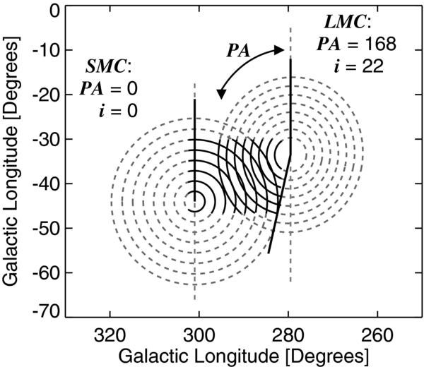
Figure 14. Schematic of the elliptical annuli used to bin the Hα intensity radially from the LMC and SMC centers. The spacing depicted between each ring is exaggerated from the actual spacing (03) used to determine the mean and median Hα intensity values. The LMC annuli is characterized by P.A. = 1680 and i = 220 and expands from the H i disk center at (l, b) = (2795, −335) (Kim et al. 1998). The SMC annuli is circular, where both P.A. = 00 and i = 00, and expands from (l, b) = (3010, −440); we chose a circular annuli because the H i gas has a random distribution that lacks a disk morphology (Stanimirović et al. 2004). The dashed gray, elliptical lines trace the complete elliptical pattern around each galaxy; the curved, black lines that overlap these gray lines mark the region covered by this survey. The P.A. of each galaxy is represented by solid black lines that diverge from the vertical axis.
Download figure:
Standard image High-resolution image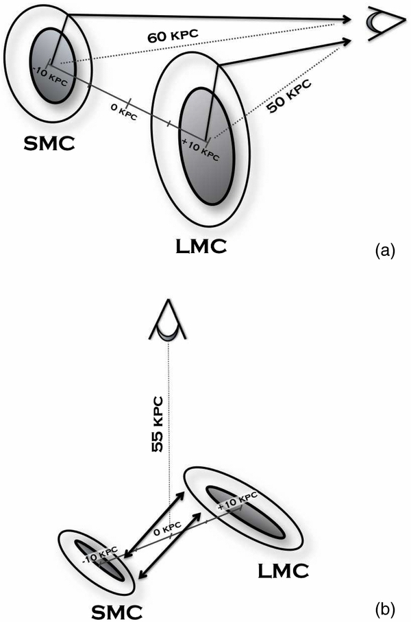
Figure 15. Schematic of the LMC and SMC orientation. Panel (a) depicts the geometry of the system, where the SMC and LMC are at a heliocentric distances of ∼60 kpc and ∼50 kpc, respectively, and are separated by ∼18.9 kpc. Panel (b) illustrates the tilt of the two galaxies with respect to each other—such that the opposite sides of their disks illuminate each other—and the observer. The O and B stellar populations within the disks of these galaxies produce the majority of the Lyman continuum emitted by these galaxies.
Download figure:
Standard image High-resolution image
Figure 16. Predicted incident ionizing radiation between the Magellanic Clouds based on the observed Hα intensity observations of the Magellanic Bridge with T = 104 K (see Equation (7)). The mean values are displayed with open circles and the median values with open squares. Typical deviations for weighted mean values are less than 0.5% and less than 15% for the median values. The vertical dashed lines indicate the center location of the SMC (assumed to be l = 302°, b = −44°, and d = 60 kpc), LMC (assumed to be l = 278°, b = −32°, and d = 50 kpc), and the Magellanic Clouds. The horizontal dashed line labels the Lyman continuum flux from the extragalactic background (Haardt & Madau 2001). The dashed-triple-dotted line marks the contribution of the Milky Way (Bland-Hawthorn & Maloney 1999, 2001) and extragalactic ionizing flux where contribution is log ΦMW + EGB = 4.73 and 4.59 photons cm−2 s−1 at the center of the SMC and LMC, respectively.
Download figure:
Standard image High-resolution image7.1. Photoionization from the Milky Way and Extragalactic Background
Bland-Hawthorn & Maloney (1999, 2001) modeled the ionizing flux radiating from the MW by assuming that the 90–912 Å radiation is dominated by O-B stars confined to spiral arms and later updated that model in Fox et al. (2005). This updated model predicts an incident ionizing flux of log (ΦMW/[photons cm−2 s−1]) = 4.33 at the center of the SMC (l = 301°, b = −44°, and d = 60 kpc) and log (ΦMW/[photons cm−2 s−1]) = 3.80 at the center of the LMC (l = 2795, b = −335, and d = 50 kpc). Haardt & Madau (2001) predict that the ionizing flux from the extragalactic background radiation is log (ΦEGB/[photons cm−2 s−1]) = 4.51 by assuming that the radiation is dominated by quasi-stellar objects, active galaxy nuclei, and active star-forming galaxies.
If photoionization is the only source of the ionization, then the incident ionizing radiation required to produce the typical Hα intensities in the central regions of the Magellanic Bridge is roughly log (ΦLC/[photons cm−2 s−1]) = 5.46, assuming the gas is at T = 104 K (see Figure 16). The photoionization from the MW and the extragalactic background, roughly log (ΦLC/[photons cm−2 s−1]) = 4.63 at the center of the Magellanic Bridge, is insufficient to produce the Hα emission alone (see Figure 16). Additional ionization must therefore come from alternative sources, including the Magellanic Clouds. If the Lyman continuum flux from the Magellanic Clouds dominates the ionization, then the Hα intensity traces the fraction of ionizing photons escaping from these galaxies.
7.2. Photoionization from the Magellanic Clouds
The Magellanic System provides us with an excellent opportunity to establish fesc for two local dwarf galaxies. If Lyman continuum radiation from the Magellanic Clouds is responsible for producing most of the ionization within the Magellanic Bridge, then the Hα emission is a direct measurement of the propagation of the ionizing radiation through this structure, see Equation (7). The LMC and SMC are at distances of roughly 50 kpc and 60 kpc, respectively. Their measured star formation rates are 0.4 and 0.2 M☉ yr−1 (Harris & Zaritsky 2009) and both galaxies have well-defined orientations with respect to each other and as observed from Earth (see Figure 15). We follow the model procedures of Bland-Hawthorn & Maloney (1999, 2002) in deriving the ionization levels in the outer disks of the LMC and SMC from their own interval UV sources and from the contribution to the mean field intensity by the other.
In the Galaxy, the total ionizing photon intensity is 2.6 × 1053 photons s−1 from a disk-averaged star formation rate of 2 ± 1 M☉ yr−1 (Williams & McKee 1997). A similar ratio of star formation rate to ionizing photon luminosity (ξ) has been measured for M82 (McLeod et al. 1993). While ξ may depend on the mean metallicity of the stellar population (e.g., Schaerer 2002), we stress that our results are mostly independent of metallicity because our star formation rates are derived from the Balmer-line intensities.
In Figure 16, we present two models for the Hα intensities derived from the outer disks of the LMC and SMC. The data for both galaxies have been binned along annuli centered at each galaxy as described by Section 7. We show both the mean and median Hα values in each annulus to demonstrate the impact of clumpiness. In our models, we have corrected for the 20% larger distance for the SMC, which largely accounts for the faster drop-off in its emission compared to the LMC, leading to the well-pronounced skewing of the U-shaped profile.
In the first model, we assume that the UV intensity arises from an inner disk of ionizing sources without the need for radiation transfer. Our conversion from ionizing flux to Hα intensities uses Equation (7), assuming T = 104 K. The first model produces an fesc of approximately 3% for the LMC and 4% for the SMC. A more complicated variation of this model, one that treats the outer H i disk as a warped structure, does not work as well (e.g., Bland-Hawthorn 1998). The fact that the first model works so well may reflect the distributed nature of the young stellar populations and the highly clumpy (fractal) nature of the ISM in both galaxies (e.g., Stanimirovic et al. 1999).
The second model is a repeat of the first model, but includes the ionizing effect of the other galaxy, i.e., the contribution of the LMC UV intensity on the outer disk of the SMC, and vice versa (see Figure 15(b)). We assume the locations in three space of both galaxies place them at both ends of an invisible cylinder 10 kpc in length. This reduces fesc, LMC to 2.5% and fesc, SMC to 2.8%. Since this value is close to the estimate derived for the first model, we conclude that fesc, LMC ≈ 3.0% ± 1.0% and fesc, SMC ≈ 4.0% ± 1.5% with a remarkable level of consistency between both methods, which does account for the uncertainty in ξ.
These models assume that photoionization is the dominant source of ionization of the Bridge. If other ionization processes also affect the Magellanic Bridge, then fesc would decrease. The dominant source of uncertainty in these fesc estimates is the uncertainty in the relative positions and orientations of these galaxies. This translates into a less certain galaxy–galaxy ionization effect. We therefore deduce that fesc, LMC < 4.0% and that fesc, SMC < 5.5%.
7.3. Photoionization from the O and B Stellar Population within the Magellanic Bridge
There are many pockets of elevated Hα emission within the Bridge that could be associated with star formation sites. Multiple studies have identified early-type stars in the direction of the Magellanic Bridge (Westerlund & Glaspey 1971; Grondin et al. 1990, 1992; Irwin et al. 1990; Demers & Irwin 1991; Demers et al. 1991; Battinelli & Demers 1998; Demers & Battinelli 1998, 1999; Harris 2007; Casetti-Dinescu et al. 2012); however, many of the studies do not distinguish A stars from the O and B stars—which produce the majority of the ionizing photons—or identify the foreground stars in their sample. The Casetti-Dinescu et al. (2012) study uses proper motions from the Southern Proper Motion Program 4 (SPM4) to select the stellar population of the Bridge, excluding foreground stars, and uses photometry from the Galaxy Evolution Explorer (GALEX) survey, the Two Micron All Sky Survey, SPM4, and the American Association of Variable Star Observers All Sky Photometric Survey to identify O and B stellar candidates. Followup spectroscopy of these candidates is still needed to confirm and place further constraints on their stellar types. The coverage of their survey spans the entire region of this Hα study.
We compare the regions of elevated Hα emission with the location of the Casetti-Dinescu et al. (2012) O and B candidates to test if they are associated with star formation sites, as illustrated in Figure 17. We quantify the elevated Hα emission by comparing the local emission with the surrounding emission through the unsharp-masked technique, creating a smoothed Hα map to half the angular resolution and dividing this smoothed map by the original map shown in Figure 7(b). Figure 17 also includes the (NUV − V)0 GALEX color for each of the candidates to indicate which stars emit more ionizing radiation and are therefore earlier-type stars. We find that although some O and B candidates do align with regions of elevated Hα emission, many locations—especially those outside the 1020 cm−2 H i contour—shows no such correlation. The locations lacking in correlation could be explained if the gas is extremely ionized or low density, although these conditions are less conducive to star formation. If the regions of the Bridge at more positive latitudes have a low density, then the cluster of three early-type stars near (l, b) = (296°, −31°) might be responsible for the latitude offset of the Hα emission from the H i emission (see Section 4), but this offset could also be caused by halo–gas interactions or by shadowing effects associated with the orientation of the Bridge with respect to the Magellanic Clouds.
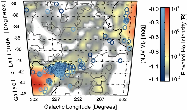
Figure 17. Regions with elevated Hα emission—compared to the neighboring sight lines—and location of the O and B stars in the Magellanic Bridge, identified through photometry and proper motions (Casetti-Dinescu et al. 2012). The shade of the blue circles denote the (NUV − V)0 color of the stars (D. I. Casetti-Dinescu 2011, private communication). We created the elevated Hα emission map using the unsharp mask technique, where the smoothed image is divided by the original image. The contour lines trace the non-extinction-corrected Hα intensity at 0.03 and 0.16 R.
Download figure:
Standard image High-resolution image
Dove & Shull (1994) found that OB associations near the solar circle produce roughly (3–4) × 1049 ionizing photons s−1. If the OB associations within the Magellanic Bridge produce ∼1049 ionizing photons s−1 and if the gas is at 104 K, then the OB associations within 1 kpc would elevate the Hα emission by 0.16 R, using Equation (7) to convert the ionizing flux to Hα intensity. However, some of the ionizing radiation will escape from the Bridge before ionizing the surrounding gas. For example, Bland-Hawthorn & Maloney (1999, 2001) estimate that 6% of the ionizing photons of the MW escapes into the halo and Section 7.2 estimates that <4% of the Lyman continuum escapes from the LMC into the surroundings and that <5.5% escapes from the SMC. The low H i column density and dust content of the Bridge would likely make this region more susceptible to losing ionizing radiation. Turbulence can also increase the ionization radiation that escapes from an OB population in the Bridge (e.g., Wood et al. 2010). The sparsity of the O and B stellar populations in the central regions of the Bridge might result in only a marginal increase in Hα emission. However, if these OB associations substantially increase the temperature of the gas, then the efficiency of producing Hα emission will decrease as IHα∝(T/104 K)−0.924; see Equation (4). In the SMC-Tail, the combination of high H i column density and high density of O and B stars will lead to enhanced Hα emission.
8. IMPLICATIONS OF THE IONIZED GAS
The fraction of UV photons that escape from galaxies, fesc, has long been recognized as an important physical quantity to measure. At high redshift, the cosmic fog of neutral hydrogen was ionized by either stars or black holes depending on the relative escape fractions of ionizing radiation with the evidence in favor of stars at present (Bromm & Yoshida 2011). At low redshift, the cosmic ionizing intensity conceivably explains the well-defined truncation observed in spiral galaxies (Bochkarev & Sunyaev 1977; Maloney 1993).
In the local universe, there are few reliable measurements of fesc because favorable geometries are called for to make this possible. Bland-Hawthorn & Maloney (1999) initially used the Magellanic Stream as a probe of the Galactic UV field until it was later discovered that in certain locations along the Stream the Hα is too bright. The high-velocity cloud population clearly establish the vertical escape fraction as ≈6% or ≈1%–2% isotropized over a sphere (Bland-Hawthorn & Maloney 2002; Putman et al. 2003a; Tufte et al. 2002). Lehnert et al. (1999) determined fesc of order a few percent from a minor axis cloud in the outer halo of M82 (the so-called cap), but this was derived from averaging the Hα emission from the cloud over its extent. Similar to the early Magellanic Stream estimates, individual clumps within the "cap" are now found to be much too bright to be explained by the central starburst. Interestingly, for both the M82 cap and the Magellanic Stream, the bright clumps can be explained in terms of slow shocks being driven into dense clumps by a fast "wind" of hot gas (Bland-Hawthorn et al. 2007; Matsubayashi et al. 2012).
There exists a small sample of dwarf starburst galaxies with estimates for fesc: NGC 5253 and Haro 11. NGC 5253 has an advantageous orientation with respect to the MW, allowing for estimates of the fesc along the minor axis of the galaxy. Zastrow et al. (2011) associate this minor axis with an ionization cone where the majority of ionization radiation escapes. If the majority of the escaping ionization radiation funnels through this cone, then fesc ≈ 3% (S. Veilleux 2012, private communication). The fesc of blue compact galaxy Haro 11—an extreme starburst dwarf—has been studied by three separate groups, each with considerably varied results. Combining International Ultraviolet Explorer spacecraft and FUSE observations, Bergvall et al. (2006) predict a 4%–10% fesc and conclude that the Lyman continuum radiation escapes through transparent windows of the ISM. Using all three channels on the Advanced Camera for Surveys on HST—covering far-UV, 2200 and U band, and optical wavelengths—the New Technology Telescope at ESO La Silla to collect Hα, Hβ, and [O iii] narrow-band images, and archival X-ray Chandra and XMM-Newton telescopes observations, Hayes et al. (2007) found a 3% fesc. They conclude that ∼90% of the ionizing photons undergo multiple resonance scattering events, masking their origin. Grimes et al. (2007) found no direct connection between outflows and escaping ionizing radiation, placing an upper limit of fesc ⩽ 2% using FUSE and Chandra observations. The contribution of ionizing photons that dwarf galaxies expel into their surroundings has yet to reach a resolution.
The circumgalactic gas structures surrounding the Magellanic Clouds provide a unique avenue for studying the ionizing radiation expelled from the Magellanic Clouds. The ionizing radiation from the MW and the extragalactic background is insufficient for producing the observed Hα emission in the Bridge. If the radiation from the Magellanic Clouds dominates the ionization in the Bridge, then the Hα emission traces the ionizing photons emitted by these galaxies. This study provides an upper limit to the fraction of escaping ionizing photons from the Magellanic Clouds as other processes may also contribute to the ionization in the Bridge. These upper limits constrain the contribution of ionizing photons in the extragalactic ionizing background that similar dwarf galaxies generate. In this way, the estimate of the fesc emitted by the LMC and SMC can anchor cosmological simulations working to identify the sources of the Lyman continuum of the extragalactic background from the epoch of reionization to today.
Besides ionizing photons, the disturbed galaxies also expel baryons into their surroundings. The Magellanic Clouds are surrounded by 6.8 × 10⁸ M☉ of neutral gas (Brüns et al. 2005). The Hα observations of the Magellanic Bridge reveal a warm ionized gas phase along the entire structure (see Figure 7(b)). In Section 6, we found that the Magellanic Bridge and the SMC-Tail contain roughly (0.7–1.7) × 108 M☉ in ionized gas and 3.3 × 10⁸ M☉ in neutral gas (see Table 3). These masses suggest that the Magellanic Bridge and the SMC-Tail have a minimum ionization fraction of 36%–52% and 5%–24%, respectively; however, these mass estimates are insensitive to the faintest and lowest density regions ( and IHα < 0.3 R) as well as the extremely ionized gas. FUSE absorption-line observations toward two early-type stars and a background quasar identified components of highly ionized gas, with ionization fractions of 70%–90%, within the Bridge (Lehner et al. 2008). The inclusion of these highly ionized components make this structure more massive and would raise the ionization fraction of the total structure.
The displacement of (4.0–5.0) × 108 M☉ of neutral and ionized gas mass from the Magellanic Clouds into the Magellanic Bridge will have repercussions on the future evolution of these galaxies that would, in all likelihood, stunt future stellar production if the material escapes the system. Including the additional neutral mass of the other circumgalactic gas structures of the Magellanic System, as determined by Brüns et al. (2005), the Magellanic Clouds have lost at least (7.5–8.5) × 108 M☉ in gas. If these other circumgalactic structures were only 25% ionized, then the total gas currently surrounding the Magellanic Clouds would exceed 109 M☉. Hα emission-line observations toward the Magellanic Stream reveal that this structure does have a warm ionized gas phase (Weiner & Williams 1996; Putman et al. 2003a; Yagi et al. 2012; G. J. Madsen 2011, private communication) and O vi absorption-line observations reveal a highly ionized component (Sembach et al. 2003; Fox et al. 2010), which increases ionization fraction of the structure and the total gas mass these galaxies have lost.
The galaxy interactions could also induce ionization of the Magellanic Bridge. The dissimilar distribution of NH i and IHα distribution in the SMC-Tail and in the Magellanic Bridge (see Figure 13(c)) suggests either that different sources ionize these structures, that they have extremely different structures, or a combination of both. In the SMC-Tail, 163 H i shells have been observed with 60% of them lacking an OB associations (Muller et al. 2003). The presence of the H i shells and active star formation could indicate that this region suffers from a combination of gravitational and pressure instabilities caused by high-velocity cloud impacts or ram-pressure effects (Muller et al. 2003), which would heat the gas and could trigger star formation. This may have created an environment ripe for the propagation of ionizing photons through the creation of large bubbles and chimneys (e.g., Norman & Ikeuchi 1989; Dove & Shull 1994; Dove et al. 2000).
The presence of young, 10–40 Myr old stars, in the central region of the Magellanic Bridge indicates that stars are actively forming in situ as they have not had enough time to migrate from the SMC (Demers & Battinelli 1998). The scarcity of metals (Lehner et al. 2008: Z ≈ 0.1 Z☉) and molecular gas (Smoker et al. 2000; Lehner 2002; Mizuno et al. 2006) within the Bridge means that the star formation may forgo traditional cooling mechanisms and may instead depend on triggering events. Young stars could spawn out of colliding cloudlets (Dyson & Hartquist 1983). Numerous simulations of the galaxy interactions provide clues on what type of events may have encouraged their formation. The Besla et al. (2012) models suggest that a violent collision could have occurred between the LMC and SMC—where the SMC traveled through the disk of the LMC, warping the disk of the LMC and shock heating the gas—and promoted star formation within the Magellanic Bridge. Once stars are formed within the Magellanic Bridge, their ionizing photons, stellar winds, and supernovae would further ionized the surrounding gas. The ram-pressure compression could also trigger star formation (Mastropietro et al. 2009), but this mechanism would not account for the lack of star formation within the Leading Arm and Magellanic Stream (Besla et al. 2012).
To further distinguish between the sources of the ionization and to further constrain the ionization fraction of the Magellanic Bridge, more observations are needed. Although the Hα observations have identified a warm ionized gas phase, they are insensitive to highly ionized and extremely low density gas. The Lehner (2002) and Lehner et al. (2008) absorption-line studies reveal that the structure, at minimal, contains pockets of highly ionized gas. At more positive latitudes, the H i column density of the Magellanic Bridge drops off before the Hα intensity decreases, suggesting that this region has a higher ionization fraction due to internal processes, such as star formation, exposure to the ionizing photons from the Magellanic Clouds, or halo–gas interactions as structure travels through the hot halo of the MW; however, this difference could also be due to the decreased sensitivity of this survey at highest velocities due to residuals left behind by a bright OH atmospheric line. To determine if a hot ionized gas phase is rampant throughout this structure, more absorption-line observations are needed toward background objects and not toward early-type stars where the presence highly ionized gas is anticipated. Additional multiline observations will aid in distinguishing between different sources of ionization as each ionization process will produce emission and absorption lines of different relative strengths.
9. SUMMARY
Using WHAM to observe the warm gas phase in the Magellanic Bridge and the SMC-Tail, we mapped the Hα emission over 350 deg2. These kinematically resolved observations—over the velocity range of +100 to +300 km s−1 in the LSR frame—include the first full Hα intensity map of the Magellanic Bridge. We compare these observations of the warm ionized gas phase with the 21 cm emission in the GASS H i survey. Through these observations, we examined the extent, morphology, velocity gradients, mass of the ionized gas, and the source of the ionization of these structures. This study finishes with the main conclusions from the Hα observations of the warm gas component in the Magellanic Bridge and the SMC-Tail.
- 1.Ionized gas mass. Three quantities dominate the uncertainty in quantifying the ionized gas mass: the distance, the morphology along the line of sight, and the distribution of ionized and neutral gas. Assuming a distance of 55 kpc, an H i line-of-sight depth that is similar to the width of the Bridge, a single component structure along each sight line, and three different distributions for the neutral and ionized gas, the mass of the ionized gas in the SMC-Tail and the Magellanic Bridge is between (0.7–1.7) × 108 M☉ compared to 3.3 × 10⁸ M☉ for the neutral mass (see Section 6 and Table 3). The Magellanic Bridge is significantly more ionized than the SMC-Tail, with the SMC-Tail at only 5%–24% ionized and the Magellanic Bridge at 36%–52% ionized. This survey is insensitive to the faintest (IHα < 30 mR) and lowest density regions. This survey is also less sensitive to Hα emission over +240 km s−1 ⩽ vLSR ⩽ +275 km s−1 velocity range because of increased residuals associated with a bright atmospheric line.
- 2.Fraction of escaping ionizing photons. The Lyman continuum from the extragalactic background and the MW produces a negligible amount of the ionization in the Magellanic Bridge. If the ionizing radiation from the Magellanic Clouds produces the majority of the ionization, then the Hα emission traces the fesc of the LMC and SMC. Assuming that the inner disk of the SMC and LMC supply the incident ionizing flux that ionizes the Magellanic Bridge and that the Magellanic Clouds ionize each other, then the LMC and SMC radiate <4.0% and <5.5% of their ionizing photons into their surroundings, respectively.
- 3.NH i and IHα distribution. There is a strong correlation between the log NH i and the log IHα near the Magellanic Clouds and within the SMC-Tail that is not observed in HVCs (see Figure 13(c)). This trend indicates that the neutral and ionized gas phases in these regions are related and affected by similar processes and could be influenced by the close proximity to the Magellanic Clouds. The contrast between the log NH i and the log IHα in the central regions on the Magellanic Bridge, shown in Figures 10 and 12, suggests that their changes are more related to the ionization fraction or to the fraction of ionized regions along the line of sight.
- 4.Velocity distribution. The global distribution of the Hα first moment map agrees with the corresponding H i map and has a relatively smooth velocity gradient of +175 to +225 km s−1 in Hα compared to +125 to +250 km s−1 in H i, as illustrated in Figure 9. This correspondence suggests that both of the neutral and ionized gas phases travel parallel to the LMC and SMC. Although the global trends of these velocity distributions agree, the intensity-weighted average Hα velocity is shifted to lower velocities and is much more smooth than the H i velocity distribution. A combination of broader Hα components and an insensitivity at highest velocities may cause these discrepancies. However, even though the velocity gradient is smooth, the spectral velocity distribution of the gas has a complex multiple component structure (see Figures 10 and 12). The strength of the Hα intensity compared to the H i column density suggests that many of these structures are predominantly ionized. In the central regions of the Magellanic Bridge, there is often additional Hα components at velocities without complementary H i emission when smoothed to the same angular resolution, which indicates the presence of distinct highly ionized structures.
The authors acknowledge helpful discussions with Nicolas Lehner, Bart Wakker, and Gurtina Besla. We thank Dana Casetti-Dinescu for providing the locations and properties of the OB stellar population in the Magellanic Bridge, Jay Gallagher for suggesting this project, and Greg Madsen for providing the developing the used Nyquist sampling routine. We also thank the anonymous referee for comments and suggestions that improved this paper. The National Science Foundation supported WHAM through grants AST 0204973, AST 0607512, and AST 1108911. K. A. Barger is further supported through NSF Astronomy and Astrophysical Postdoctoral Fellowship award AST 1203059. J. Bland-Hawthorn acknowledges a Federation Fellowship from the Australian Research Council.
Facility: WHAM - Wisconsin H-Alpha Mapper
Footnotes
- 4
1 Rayleigh = 106/4π photons cm−2 sr−1 s−1, which is ∼1.7 × 10⁻⁶ erg cm−2 s−1 sr−1 at Hα.