


ABSTRACT
The solar cycle has a profound influence on the solar wind (SW) interaction with the local interstellar medium (LISM) on more than one timescales. Also, there are substantial differences in individual solar cycle lengths and SW behavior within them. The presence of a slow SW belt, with a variable latitudinal extent changing within each solar cycle from rather small angles to 90°, separated from the fast wind that originates at coronal holes substantially affects plasma in the inner heliosheath (IHS)—the SW region between the termination shock (TS) and the heliopause (HP). The solar cycle may be the reason why the complicated flow structure is observed in the IHS by Voyager 1. In this paper, we show that a substantial decrease in the SW ram pressure observed by Ulysses between the TS crossings by Voyager 1 and 2 contributes significantly to the difference in the heliocentric distances at which these crossings occurred. The Ulysses spacecraft is the source of valuable information about the three-dimensional and time-dependent properties of the SW. Its unique fast latitudinal scans of the SW regions make it possible to create a solar cycle model based on the spacecraft in situ measurements. On the basis of our analysis of the Ulysses data over the entire life of the mission, we generated time-dependent boundary conditions at 10 AU from the Sun and applied our MHD-neutral model to perform a numerical simulation of the SW–LISM interaction. We analyzed the global variations in the interaction pattern, the excursions of the TS and the HP, and the details of the plasma and magnetic field distributions in the IHS. Numerical results are compared with Voyager data as functions of time in the spacecraft frame. We discuss solar cycle effects which may be reasons for the recent decrease in the TS particles (ions accelerated to anomalous cosmic-ray energies) flux observed by Voyager 1.
Export citation and abstract BibTeX RIS
1. INTRODUCTION
The solar wind (SW) interaction with the local interstellar medium (LISM) is an exciting area of space physics research that embraces different time and length scales. From the gas dynamic (or magnetohydrodynamic, MHD) perspective, it is a combination of jet and blunt body flows (Wallis & Dryer 1976) which involves a tangential discontinuity (the heliopause, HP), separating the SW from the LISM, a SW termination shock (TS), and possibly a LISM bow shock (BS). Since the LISM flow, according to the He atom velocity and temperature determinations from different observational sources (Witte et al. 1993; Witte 2004; Möbius et al. 2004, 2012) is supersonic, the BS can exist only if the interstellar magnetic field (ISMF) is sufficiently weak. If it were not for the LISM plasma heating by charge exchange between the pristine LISM protons and secondary H atoms born in the SW and moving upstream the LISM, the answer to the question about the BS existence would be easy without any numerical simulation by a direct calculation of the fast magnetosonic Mach number in the unperturbed LISM. The LISM proton heating, however, can be substantial (above 8000 K) and depends on the LISM plasma density (McComas et al. 2012). Numerical investigations by Heerikhuisen & Pogorelov (2011) show that the ISMF strength, B∞, should be below 3 μG to reproduce the shape and position of the Interstellar Boundary Explorer (IBEX) ribbon—a narrow region of the enhanced flux of energetic neutral atoms (ENAs) on the celestial sphere. MHD simulation results presented in Zank et al. (2013) show that Lyα absorption observations in the directions of nearby star are consistent with B∞ ≈ 3 μG. The heliotail is known to be affected by the ISMF strength and direction (Pogorelov et al. 2004), but the effect is smaller in the presence of interstellar H atoms (Pogorelov et al. 2006, 2008, 2009b). This agrees with the recent analysis performed by McComas et al. (2013), which is based on enhanced statistics from the first three years of IBEX observations. These results show that the heliotail has a complex structure including two lobes, one of which was previously identified (Schwadron et al. 2011) as an offset heliotail.
Voyager 1 and 2 (V1 and V2) crossed the heliospheric TS in 2004 December and in 2007 August, respectively (Stone et al. 2005, 2008; Richardson et al. 2008), and after 35 yr of historic discoveries, are approaching the HP. They acquire in situ information about the local properties of the SW plasma, energetic particles, and the magnetic field at the heliospheric boundary. As the twin Voyager spacecrafts move toward the HP, they continue to return new and often puzzling measurements of the SW protons, energetic particles, and magnetic field that often differ markedly between the two spacecrafts. A remarkable example is the identification of a surprising radial velocity, vR, profile in the inner heliosheath (IHS) at V1 (Krimigis et al. 2011). It exhibits a substantial negative time gradient of vR since mid-2007, so that vR has decreased to zero and ultimately acquired negative values. Moreover, recent analysis of the energetic particle anisotropies with the V1 low-energy charged particle data suggests that the latitudinal velocity component is very small, while the azimuthal component grew to values comparable with vR (Decker et al. 2012). It is hard to explain the behavior of the SW velocity in the framework of a steady-state SW–LISM interaction model. V1 observations also fundamentally differ from the V2 plasma measurements that exhibit a gradual decrease in vR accompanied by the growth of the latitudinal velocity component and an increase in the plasma density (Richardson 2011; Richardson & Wang 2012).
In preceding papers (Pogorelov et al. 2004, 2006, 2009a), hereafter referred to as Paper I, Paper II, and Paper III, respectively, we considered three-dimensional (3D) features of the outer heliosphere due to coupling between the SMF and interplanetary magnetic field (IMF) in the MHD and multi-fluid formulations for different ISMF orientations, assuming both steady and unsteady SW flows. In particular, Paper III dealt with the effects of solar rotation and solar cycle. Although the cycle model was oversimplified, its application made it possible to identify unusual behavior of the SW radial velocity in the vicinity of the HP. Extended regions of negative vR have been found in the IHS that extended ∼20 AU inside the HP. On the other hand, the distributions in the outer heliosheath (OHS) showed the areas of positive vR extending ∼50 AU into the OHS. Further analysis of this phenomenon performed by Pogorelov et al. (2012) showed that V1 was more likely to observe the regions of negative vR than V2. V1 observations of very small and then negative radial velocity components were accompanied by nearly zero latitudinal component, and a large transverse component (Decker et al. 2012). It appears that qualitatively very similar flow characteristics can be obtained if solar cycle effects are taken into account. Even a simplified solar cycle model from Paper III allowed us to explain many features of the observed plasma flow. Our simulations showed that the radial component of the SW velocity in the IHS starts to decrease more rapidly once the plasma enters a magnetic barrier. These barriers lie outside the IHS region covered by the wavy current sheet (plasma β inside such barriers is ∼5). The width of a magnetic barrier and its ability to decelerate the SW flow appeared to be functions of the solar cycle. We showed that the regions of negative vR are time-dependent and their spatial variation is closely related to the slow and fast wind interaction as the latitudinal extent of slow wind increases from solar minimum to solar maximum and the unipolar magnetic field region displaces the region of alternating polarity separated by the heliospheric current sheet (HCS). Slow and fast streams move on the opposite sides of the magnetic barrier. Negative vR is observed at the edge of such magnetic barrier when the plasma flowing on barrier's outer side starts moving over it. Numerical simulations show that the presence of negative vR is not due to the HP motion, as one would expect without solving the coupled system of MHD and gas dynamic equations (see Papers I and II for more details).
Here, we describe a more realistic SW model based on Ulysses observations and use it to model the SW–LISM interaction.
Ulysses is a unique heliophysics spacecraft (Poletto & Suess 2004; Balogh et al. 2008) that has accumulated exactly the kind of data one needs to create a time-dependent model which takes into account the effects of the Sun's rotation and solar cycle. Launched in 1990 October, Ulysses provided pole-to-pole SW observations until 2009 (Phillips et al. 1995a, 1995b; Riley et al. 1997; McComas et al. 1996, 2000b, 2000a, 2002, 2003, 2006, 2008; Smith et al. 2003; Poletto & Suess 2004; Balogh et al. 2008). All other spacecrafts to date had trajectories relatively close to the ecliptic plane, so Ulysses single-handedly explored the previously unsampled mid- and high-latitude heliosphere. Over the 18 yr of the mission, Ulysses completed orbits over both poles roughly every 6 years. McComas et al. (2000a) presented the SW observations over Ulysses' first full polar orbit in a form of latitudinal approximations. The SW plasma properties were discovered to depend on latitude, with the high-latitude wind dominated by fast coronal hole (CH) streams, whereas the flow at low latitudes originates in closed coronal magnetic field regions and is considerably slower and less dense. At mid-latitudes, Ulysses repeatedly traversed a large, stable corotating interaction region (CIR; see Gosling 1996 and references therein) formed by the interaction of slow wind and faster polar coronal hole (PCH) wind overtaking it. Around solar minimum, the band of SW variability was narrow, and confined to within a few tens of degrees of the heliographic equator (McComas et al. 1998). The results from the second orbit showed a much more complex structure of the 3D SW at all heliolatitudes (McComas et al. 2002; Neugebauer et al. 2002). McComas et al. (2006) examined observations of the SW during Ulysses' second orbit and found the stream structure remarkably different and more variable than that observed during Ulysses' first orbit. The proposed explanation is a more complicated HCS structure, including both larger average HCS tilt and a significant warping structure of the belt of low-speed flow. McComas et al. (2008), by analyzing the SW observations from both large PCHs during Ulysses' third orbit, showed that the fast SW was slightly slower, significantly less dense, cooler, and had less mass and momentum flux than during the previous solar minimum (first) orbit. In addition, while much more variable, the measurements in the slower, in-ecliptic wind match quantitatively with the earlier Ulysses data and show essentially identical trends. Thus, these combined observations indicate significant, long-term variations in SW output from the entire Sun. The significant, long-term trend to lower dynamic pressures means that the heliosphere has been shrinking and the HP must have been moving inward. In addition, their observations suggest a significant and global reduction in the mass and energy fed into the SW below the sonic point in the corona.
Our physical model (see the reviews of Pogorelov et al. 2009c; Zank et al. 2009) and the corresponding package of adaptive mesh refinement numerical codes supporting it (hereafter referred to as Multi-Scale FLUid-Kinetic Simulation Suite) uses an MHD treatment of ions and kinetic (or multi-fluid) modeling of neutral particles penetrating into the heliosphere, and addresses the complexity of charge-exchange processes and ISMF–IMF coupling at the heliospheric interface. It is capable of performing detailed calculations of the nonstationary SW–LISM interaction. It has been used to analyze the influence of the interstellar environment on the heliospheric interface and allowed us to investigate the interaction regimes with nonzero angle between the Sun's magnetic and rotational axes. This model was compared with the first IBEX measurements (McComas et al. 2009; Schwadron et al. 2009) and reproduced the ENA ribbon (Heerikhuisen et al. 2010). Our dynamical model of the heliosphere allows us to create time-dependent ENA maps and compare them with the IBEX measurements, which have already exhibited variability in ENA fluxes and in the ribbon position (McComas et al. 2010). Fitting the observed ribbon with the model simulations (Pogorelov et al. 2010; Heerikhuisen & Pogorelov 2011) helps to identify the ISMF orientation which affects the heliospheric interface considerably. Pogorelov et al. (2011) showed that solar cycle is clearly seen in the distributions of plasma density on the surface where the lines of sight are perpendicular to the ISMF lines in the OHS (B · R = 0), which makes solar cycle simulations particularly interesting. Note that those directions correlate (McComas et al. 2009; Frisch et al. 2010) with the directions toward the IBEX ribbon in the model of Pogorelov et al. (2009b).
Paper III considered a nominal solar cycle by assuming it to be exactly periodic with the period equal to 11 yr. The SW velocity in the fast and slow wind regions were assumed to be constant, and only the boundary between them had the latitudinal extent changing from 35° at minima to 80° at maxima. The Sun's rotation and magnetic-dipole axes never coincided. For this reason, the HCS, which separates the SW into regions of opposite interplanetary magnetic field (IMF) polarity, has a complicated wavy shape. IMF polarity changes related to a 25 day solar rotation period were first identified from IMP-1 observations by Ness & Wilcox (1964, 1965). Definitive evidence of the inclined HCS (with dependence on the heliographic latitude) was provided by Pioneer 11 (Smith et al. 1978). An extensive analysis of the HCS behavior at distances covered by the Ulysses trajectory was undertaken by Smith (2001). The HCS is also seen in Voyager observations (Burlaga et al. 1977; Klein & Burlaga 1980; Burlaga & Ness 2011). Paper III treated the HCS as a strictly periodic structure related to a constant solar rotation period with the latitudinal extent varying from 8° at minima to 80° at maxima. Additionally, in the approximation of a rotating magnetic dipole we assumed that the IMF polarity changes to the opposite every 11 yr. The approach in Paper III allowed us to identify many systematic features related to solar cycle effects. Besides, the assumption of a constant period allowed us to investigate the cycle accumulation effects. In particular, we found that 30–50 repeated solar cycles are necessary to saturate the solution to a condition where it becomes entirely periodic. This contrasted with the two-dimensional (2D), fluid-kinetic, solar cycle simulations of Izmodenov et al. (2005), who assumed a 66 yr periodicity to avoid statistical noise in the stochastically generated collisional source term.
The aim of this investigation is to analyze the effects of the solar cycle using a model based on Ulysses observations. The paper is structured as follows. Section 2 describes the physical model, which is used in our numerical simulations, its accuracy, and validation. In Section 3, the results obtained are analyzed. In Section 4, we summarize our findings.
2. PHYSICAL MODEL AND BOUNDARY CONDITIONS
Numerical results presented in this paper are obtained assuming that the flow of charged particles is described by ideal MHD equations with source terms describing charge exchange between ions and neutral atoms. The transport of neutral atoms is modeled using a multi-fluid model, where different populations of neutral hydrogen (H) atoms are described by different sets of the Euler gas dynamics equations, again with the appropriate charge-exchange source terms. The basics of our multi-fluid model are described in Pauls et al. (1995) and Zank et al. (1996b). An MHD-neutral implementation and its comparison with the MHD-plasma/kinetic neutrals simulations of Heerikhuisen et al. (2007, 2008) are presented in Paper II and in Pogorelov et al. (2009c). From the viewpoint of the plasma distributions, the differences are only quantitative and therefore can be addressed, in the framework of this study, by adjusting unknown properties of the LISM, such as the proton and H atom densities. This is supported by an important, extensive comparative analysis of different axially symmetric SW–LISM interaction models performed by Müller et al. (2008).
The solar cycle description used here employs Ulysses measurements to obtain time-dependent boundary conditions at the inner boundary. Each time observations are available at a single spacecraft location only, while we need time-dependent distributions at a fixed distance from the Sun, which requires additional analysis.
We create our time-dependent boundary conditions using Ulysses observations between 1991 January 15 and 2010 December 15. It is further assumed that the latitudinal extent of slow SW is a function of time and can be asymmetric with respect to the solar equatorial plane. It is assumed that at 10 AU, the SW is axially symmetric with respect to the Sun's rotation axis. Thus, there is no dependence of the plasma distributions on the azimuthal angle ϕ at the inner boundary. We derive the sets of data for the SW radial velocity component, number density, and temperature. Each of the data sets has latitudinal resolution of 1° and expands through the interval between the minimum of SC22 to the minimum of SC23. The time resolution is one month, so that we have 240 different moments in time, numbered across the time interval 1 ⩽ nt ⩽ 240, in our data sets.
To build up an empirical description of the solar cycle, times are identified at which SW evolution changes character, the wind variation with latitude is described at those times, and interpolations are made in between. Below we describe the initial data and 15 basic moments of time. The data are first linearly interpolated between each of the assigned data points, which are then slightly smoothed with a 4 months × 4° moving boxcar average that tapers off at the edges of arrays to avoid extreme jumps. In this way, we produce data at 1 AU. To shift the boundary conditions to 10 AU, we use a slightly modified version of the formulae from Ebert et al. (2009) which approximate the radial and latitudinal SW behavior in the fast and slow wind.
Each of the assigned data first uses the approximation results at the minima of SC22 and SC23. Subsequently, the Wilcox Solar Observatory (WSO) 2.5 solar radii potential field source surface (PFSS) plots are used to infer how the speed profiles are modified in latitude, initially, as the sunspot cycle rises toward the sunspot maximum and, finally, as the cycle returns to minimum. The rise and fall are asymmetric in time. The SC23 minimum is also asymmetric in latitude. There are occasional long-lasting (more than ∼3 months) periods during the cycle when the current sheet diverges from the underlying systematic changes over the sunspot cycle, leading to significant differences from a simple sinusoidal variation.
We outline the derivation of the radial velocity profiles first.
1991 January 15 (nt = 0). The first Carrington rotation (CR) is copied from nt = 60. We use the Ebert et al. (2009) formulae for slow and fast wind, which give us the following radial velocity magnitudes (in km s−1):
These values are kept constant until 1996 January 15 (nt = 60). The next basic point is on 1996 June 15 (nt = 65), where
This means that the latitudinal extent of slow wind is 21°.
1996 October 15 (nt = 69). This is the Zürich relative sunspot number (Rz) minimum for sunspot cycle 23. The formal values given here by Ebert et al. (2009) are slightly modified to take into account that we have the configuration with a ±20° slot for slow wind with rotational modulation between ±20° and ±37°, which is seen from Figure 1. Looking at the corresponding PFSS plot, we identify a ±25° wiggle in the HCS. This broadens the low-speed region and causes rotational modulation up to higher latitudes. It appeared in 1996 August and was much reduced by 1997 February–April. It came back in 1997 August. Our modified choice is
1997 August 15 (nt = 79).
1998 February 15 (nt = 85). Since 1998 January 15, the HCS tilt and complexity start increasing and there appears a significant HCS tilt. The geometry also becomes north–south (N-S) asymmetric. We therefore choose
1998 September 15 (nt = 92). This time should be between the maximum profile and nt = 85. It is N-S symmetric, but with a big quadrupole component of magnetic field. Thus,
1998 December 15 (nt = 95). The HCS reaches high latitudes. There remains little fast wind, but still more in the south than in the north. Thus,
1999 June 15 (nt = 101). The maximum conditions are achieved. There are hardly any polar holes, so we specify
2000 March 15 (nt = 110). We have the Rz maximum time for sunspot cycle 23. The SW speed around that time, from Ulysses, is shown in Figure 2. A good estimate for 2000.3 is to take vR = 400 km s−1 at all latitudes. This ignores rotational modulation. The north polar hole developed early in this cycle, so some asymmetry should be expected. Thus, we put in some asymmetry in the CH formation during the declining phase, the northern CH growing earlier and faster. At maximum, let

Figure 1. Distribution of the SW radial velocity component at Ulysses between the years of 1994.33 and 1996 (black line), and the spacecraft latitude (blue line). Observational data are from the SWOOPS instrument on board Ulysses.
Download figure:
Standard image High-resolution image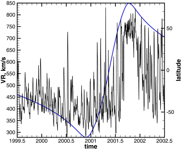
Figure 2. Distribution of the SW radial velocity component at Ulysses between the years of 1999.5 and 2002.5 (black line), and the spacecraft latitude (blue line). Observational data are from the SWOOPS instrument on board Ulysses.
Download figure:
Standard image High-resolution imageBy 2001 September, the southern coronal hole (S-CH) must have formed because there is a clear rotational modulation of the speed when Ulysses was at −80°. The modulation grows until Ulysses reaches approximately −10°, but the speed is below 700 km s−1. Continuous fast wind is encountered at ∼2001.7, above ∼70°.
2001 March 15 (nt = 122).
2001 September 15 (nt = 128).
The polar holes continue growing asymmetrically since they arrive at an asymmetrical situation in 2008.
2003 June 15 (nt = 149). Now the magnetic field is observed to be almost a pure tilted dipole. The S-CH is down to ∼−60°, while the N-CH is up to ∼50°. The fast wind from the N-CH is in the southern hemisphere, and vice versa. There is no extremely slow wind velocities. Thus,
2004 September 15 (nt = 164). A remarkable quadrupole component develops and persists (see, e.g., CR2021), with variations, during 2005–2007 as the HCS tilt decreases. This reduces speeds around the equator. The S-CH appears to be somewhat larger than the N-CH now. So
2007 February 15 (nt = 193). The N-CH is again larger than the S-CH (CR2053). Thus,

2008 December 15 (nt = 215). This is the estimated Rz minimum for sunspot cycle 24. The SW speed around this time is shown in Figure 3. The latitudinal distribution is asymmetric, both in the boundaries for the slow wind and in the rate of rise out of the slow wind. We include a small modification to the Ebert et al. (2009) formulae to take into account this asymmetry
2010 December 15 (nt = 239). The distribution is taken directly from Ebert et al. (2009) on 2008 December 15 as corresponding to the sunspot minimum and the key time for the SC23 minimum profiles:

Figure 3. Distribution of the SW radial velocity component at Ulysses between the years of 2006.8 and 2008.6 (black line), and the spacecraft latitude (blue line). Observational data are from the SWOOPS instrument on board Ulysses.
Download figure:
Standard image High-resolution imageTo extrapolate the speed to 10 AU, we first define "fast wind" as that with vR ⩾ 500 km s−1 and "slow wind" as that with vR < 500 km s−1. According to Ebert et al. (2009), vR ∼ R0.003 in the fast wind in 1996 and ∼R0.01 in 2008. These dependencies are weak, but to provide some increase in speed with distance, we use the mean of these exponents: vR ∼ R0.006 for all fast wind, for all times. In the slow wind, Ebert et al. (2009) give the same radial dependence for slow wind in both 1996 and in 2008, which is vR ∼ R0.048.
It is a little more difficult to extrapolate temperature and density to 10 AU. Instead of deriving them using the PFSS models, we use a modified version of the Ebert et al. (2009) relationships SC22 and SC23. These are linear relationships between speed and density (or temperature), but they are different depending on whether it is fast wind or slow wind. The difficulty is that density and temperature dependencies on speed are significantly different for SC23 than for SC22. This is clear, of course, from the radically different SW conditions for the SC23 minimum than in earlier minima. The density is lower, besides simply being relatively lower along with the speed. We use the linear relationships for SC22 up until sunspot maximum in 2000 March. After that, we use a linear (with time) conversion to the SC23 linear relationships from those for SC22, with the SC23 relationships being fully achieved at the SC23 minimum (taken here to be 2008 December).
The Ebert et al. (2009) relations are altered in the following way.
- 1.The radial dependency of density in fast wind is R−1.93 in SC22 and R−1.68 in SC23. Not only is the latter dependence not mass-conserving, it allows the SW density around 1–2 AU at SC22 to be less than the SW density at 10 AU at SC23. We therefore decided to use the dependence R−1.93 for both SC22 and SC23 in fast wind. Slow wind behaves as R−1.93 in both cycles.
- 2.The latitudinal dependency of the speed in slow wind, as given in Ebert et al. (2009) for both cycles, may lead to a possible non-physical consequence when extrapolated to high latitudes near sunspot maximum, i.e., slow wind may acquire negative densities. Such dependency may exist near the current sheet near sunspot minimum, but is unlikely at large distances from the current sheet. We arbitrarily reduced this dependence in both cycles.
Let us start with the Ebert et al. (2009) formulae with the above-mentioned modifications.
For SC22, we have
- 1.Slow wind (vR < 500 km s−1)

- 2.Fast wind (vR ⩾ 500 km s−1)


For SC23, we have
- 1.Slow wind (vR < 450 km s−1)
- 2.Fast wind (vR ⩾ 450 km s−1)


Combining these relations to eliminate θ gives for SC22
- 1.Slow wind
- 2.Fast wind
The similar correlation equations for SC23 read
- 1.Slow wind
- 2.Fast wind

The resulting distributions of the SW density and velocity at 10 AU are shown in Figure 4 as 2D plots depending on time t and latitude θ. The tilt of the Sun's magnetic axis is a function of time taken from the WSO Web site. The tilt dependence on time is presented in Figure 5. At this stage, we neglect CIRs assuming that major stream interaction finished by 10 AU. CIRs are transition regions between fast and slow SW directly measured by Ulysses (Gosling et al. 1993). It is known that at heliocentric distances greater than 8 AU CIRs start to collide and merge, thus producing so-called corotating merged interaction regions (CMIRs; Burlaga et al. 1983). Numerical simulations in Borovikov et al. (2012) show that such CMIRs may indeed influence the SW flow even in the IHS. A more detailed description of the CIR behavior as a function of solar cycle will be considered elsewhere. To obtain an initial steady state, we keep the SW boundary conditions at t = 0 as long as it is necessary to make the time derivative negligible.

Figure 4. Distributions of the SW density in cm−3 and velocity in km s−1 as a function of the latitude angle θ and time in years.
Download figure:
Standard image High-resolution image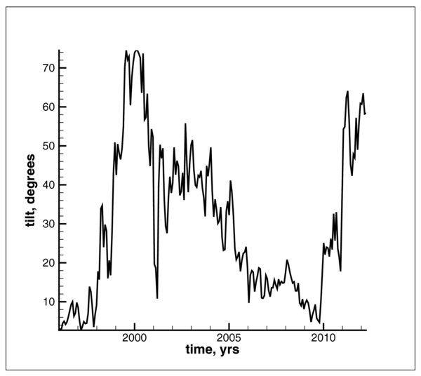
Figure 5. Angle between the Sun's magnetic and rotation axes from the Wilcox Solar Observatory data.
Download figure:
Standard image High-resolution imageThere are no in situ measurements of the LISM properties, although its velocity and temperature can be deduced from neutral He measurements (Witte et al. 1993; Witte 2004; Möbius et al. 2004, 2012). We assume here that the velocity, plasma density, and temperature of the unperturbed LISM are the following: V∞ = 26.4 km s−1, T∞ = 6527 K, and n∞ = 0.06 cm−3. The first two quantities are derived from different He atom observations and summarized in Möbius et al. (2004). According to Möbius et al. (2012), these quantities, especially the direction and magnitude of V∞, may be somewhat different. The effect of the direction change should be small as the difference is less than 3°. The effect of smaller V∞ should be compensated by a proper increase in n∞. The LISM proton density is a free parameter in the range 0.004 ⩽ n∞ ⩽ 0.14, according to Vallerga (1996), where it is also estimated that the H atom density should be in the range 0.15 ⩽ nH∞ ⩽ 0.34. We are not investigating the dependence of the solution on the neutral H density nH∞ or the ISMF vector B∞, which was done in Heerikhuisen & Pogorelov (2011).
The notion of the hydrogen deflection plane (HDP) has become common since the publication of the Lyα backscattered emission results in the context of the ISMF vector B∞ orientation (Lallement et al. 2005). It was suggested in that paper that the deflection of the neutral H flow direction from the neutral He flow direction in the inner heliosphere (less than 10 AU from the Sun) is due to the action of the ISMF. If the SW is spherically symmetric and the IMF is absent, the deflection of neutral H occurs exactly in the plane formed by B∞ and V∞. We call it the B–V plane. Pogorelov et al. (2008, 2009b) showed that the deflection is predominantly in the B–V plane even in the presence of the IMF. Our choice of B∞ belonging to the HDP allowed us to fit the ribbon of enhanced energetic neutral atom flux observed by the IBEX (McComas et al. 2009; Heerikhuisen et al. 2010). Moreover, Heerikhuisen & Pogorelov (2011) showed that the position of the ribbon on the celestial sphere strongly depends on the orientation of the B–V plane. We therefore choose B∞ in the HDP plane at 30° to V∞. We choose a Cartesian coordinate system with the origin at the Sun, its z-axis being aligned with the Sun's rotation axis. The x-axis belongs to the plane determined by the z-axis and V∞ and is directed upwind into the LISM. The y-axis completes the right coordinate system.
We use a one-fluid approximation for charged particles, i.e., the presence of pickup ions (PUIs), which are created in all regions of the heliosphere when neutral particles exchange charge with ions, is taken into account approximately by assuming that PUIs, on average, quickly acquire the velocity of the ambient SW and that the effective temperature of the ion mixture is determined by the sum of the internal energies of PUIs and thermal core ions. This simple model is sufficient to describe the TS response to solar cycle variations.
3. HELIOSPHERIC RESPONSE TO SOLAR CYCLE VARIATIONS
The solar cycle plays an important role in the distribution of the heliospheric quantities, which is obvious even from simplified models (Pogorelov 1995; Tanaka & Washimi 1999; Zank & Müller 2003; Scherer & Fahr 2003; Scherer & Ferreira 2005; Izmodenov et al. 2005; Sternal et al. 2008; Pogorelov et al. 2009b). Moreover, the first two ENA maps created by IBEX show a strong dependence of the ENA flux on time (McComas et al. 2010). Since one full ENA map is created by IBEX every six months, the solar cycle dependence may be resolved in more detail than shorter timescales related to the Sun's rotation and SW transients (Pogorelov et al. 2011). In this section, we use our simulations of the solar cycle based on the Ulysses data to analyze the TS behavior, as well as the distributions of the SW plasma and IMF.
Figure 6 shows the evolution of the plasma radial velocity. Numerical simulations do not extend to the current time because of the end of the Ulysses mission on 2009 June 30. The initial frame corresponds to the data derived from the first Ulysses orbit. The boundaries between the fast and slow wind are clearly seen because we assumed a narrow transition region between them. Near the solar maximum the latitudinal extent of slow wind becomes close to 90°. Comparison of the first and last time frames in Figure 6, and a similar frame in Figure 10, shows that the TS heliocentric distances decreased in all latitudinal directions by the end of the Ulysses mission. This is due to a substantial decrease in the SW ram pressure reported by McComas et al. (2008). We will discuss the effect of this asymmetry on the heliocentric distances at which V1 and V2 crossed the TS later, when analyzing the linear distributions along the spacecraft trajectories.

Figure 6. Evolution of the radial velocity component in the meridional plane. The distances are given in AU and velocity in km s−1. The actual date of each snapshot is given in the right upper corner.
Download figure:
Standard image High-resolution imageFigure 7 shows the time evolution of the plasma density at the same time as in Figure 6. We also added a black line to this figure which separates the regions of positive and negative radial velocity components vR. It is clear from these figures that regions of negative vR are observed at Voyager latitudes in the vicinity of the solar minimum, especially after the latitudinal extent of the slow wind starts growing. Negative vR was observed by V1 for about 1.5 yr (Krimigis et al. 2011) and it continues to be very small as compared with the other spherical velocity components now. This takes us to the explanation of a nearly vanished intensity of the TS particles at V1, which has been observed since 2012 September. One explanation of this phenomenon was proposed by McComas & Schwadron (2012) and is based on the end of the direct connection of the observational point from the TS. According to McComas & Schwadron (2006), SW ions are easily injected into the acceleration process at the TS flanks, where the angle between the shock normal and the corresponding magnetic field line is not close to 90°. These ions may then move along this magnetic field to the spacecraft location. If the V1–TS connection is not "direct," i.e., a corresponding IMF line makes more than one full rotation about the z-axis (see Pogorelov et al. 2007), the ions cannot reach the observational point due to the scattering and diffusion processes. This means that the source of the TS particles disappears. One argument against the McComas & Schwadron (2012) scenario might be the ability of accelerated ions to convect toward the HP with magnetic field lines they populate. However, V1 is measuring vR ⩽ 0, which means that such convection is not possible. Moreover, nonpositive vR means that V1 is in fact crossing magnetic field lines that originated at considerably lower latitudes (see Pogorelov et al. 2012). It is clear that such field lines should perform very many rotations about the z-axis until they reach the spacecraft, which gives strong arguments in favor of the McComas & Schwadron (2012) mechanism, although at a somewhat more sophisticated level that includes 3D and time-dependent effects. In this sense, there indeed seems to exist a pronounced boundary between two regions in the vicinity of the HP. Inside this boundary, V1 is directly connected to the TS, the source of the TS particles is available, and their energy spectrum is unrolling. On the other side of this boundary, V1 starts sampling magnetic field lines that originated at lower latitudes, which can be disconnected from the TS for so long that their convection with the SW velocity is insufficient to preserve any substantial termination shock particle (TSP) flux.
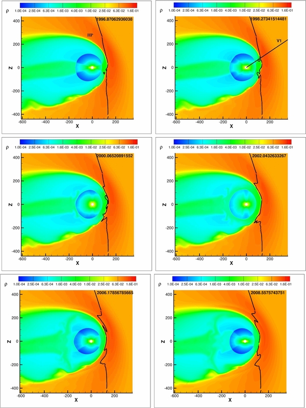
Figure 7. Evolution of the plasma density in the meridional plane. The distances are given in AU and density in cm−3. The actual date of each snapshot is given in the right upper corner.
Download figure:
Standard image High-resolution imageOf particular interest is the evolution of magnetic field in the heliosheath. It is shown in Figures 8 and 9. In contrast to our previous simulations performed with a simple sinusoidal variation of the angle between the Sun's magnetic and rotation axes (Pogorelov et al. 2009a), the choice of a realistic tilt results in magnetic barriers which have a layered structure. Further investigation of this phenomenon is necessary with a more detailed resolution of the HCS, which represents a sort of magnetic equator for the IMF. The HCS can be reproduced numerically, with some accuracy, until the SW velocity becomes small (Borovikov et al. 2011). This smallness is defined either by numerical resolution or by the scale of turbulence intrinsic to the SW flow in the IHS (Lazarian & Opher 2009; Drake et al. 2010). An alternative to this is to consider the HCS as a surface passively propagating with the SW flow (Czechowski et al. 2010; Borovikov et al. 2011). This automatically implies the assumption of a fixed polarity of the IMF. As the IMF polarity is known to change with an approximately 22 yr period, such choice is not obvious. Moreover, the choice of a sign for the unipolar field affects coupling of the ISMF and IMF at the HP substantially and may affect magnetic reconnection which is likely to occur across the HP. The effect of magnetic reconnection at the HCS and HP may be investigated in a global setting and in a realistic IHS. This is plausible because the Lazarian & Vishniac (1999) model predicts that for a sufficiently high level of turbulence, collisional and collisionless fluids should reconnect at the same rate. A detailed discussion on the relationship of turbulence and kinetic effects within the Lazarian & Vishniac (1999) model is presented by Eyink et al. (2011). The rapid reconnection of magnetic-flux structures with dimensions considerably exceeding the gyroradius requires a breakdown in the standard Alfvén flux-freezing law. Eyink et al. (2011) developed predictions based on the phenomenological (Goldreich & Sridhar 1995) theory of strong turbulence and weak MHD turbulence, and recovered the predictions of the Lazarian & Vishniac (1999) theory for the reconnection rates of large-scale magnetic structures. SW flow in the IHS shows features of preexisting turbulence (Burlaga & Ness 2009) which must be taken into account when investigating reconnection in the HP vicinity (both at the compressed HCS and due to coupling between the ISMF and IMF). Lapenta & Lazarian (2012) recently considered the relation between the Lazarian & Vishniac (1999) turbulent reconnection theory and numerical experiments (Lapenta 2008; Skender & Lapenta 2010) and demonstrated the spontaneous onset of turbulent reconnection in systems that were initially laminar.

Figure 8. Evolution of the magnetic field strength in the meridional plane. The distances are given in AU and the magnetic field in μG. The actual date of each snapshot is given in the right upper corner.
Download figure:
Standard image High-resolution image
Figure 9. Evolution of the y-component (into the figure plane) of the magnetic field vector in the meridional plane. The distances are given in AU and the magnetic field in μG. The actual date of each snapshot is given in the right upper corner.
Download figure:
Standard image High-resolution imageThe distributions of some plasma and magnetic field quantities at the end of the Ulysses mission are shown in Figure 10. To analyze them in more detail, we will consider the distributions along the V1 and V2 trajectories as functions of time t (see Figures 11 and 12). Note that we use the real physical positions of the spacecraft in time. The analysis of the velocity distributions leads us to the following conclusion. In our simulation, V1 crossed the TS at the end of 2004 April, at a distance of about 91.9 AU. The real crossing occurred in 2004 December at ≈94 AU. According to our results, at the moment of the V1 crossing, the TS position in the V2 direction was at approximately 86 AU. This means that the V1–V2 asymmetry of the TS was rather large in 2004.
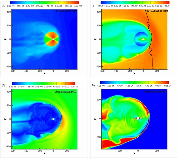
Figure 10. Evolution of the radial velocity component, plasma density, magnetic field magnitude, and its y-component in the meridional plane in 2010.07.
Download figure:
Standard image High-resolution image
Figure 11. Top row and the left panel in the bottom row: time variation of the R-, T-, and N-components of the magnetic field vector along the V2 trajectory (black lines). Bottom row, right panel: the distribution of the radial component of the plasma velocity vector along the V2 (black line) and V1 (red line) trajectories. Voyager observations are shown with blue lines in all panels.
Download figure:
Standard image High-resolution image
Figure 12. Top row: the distributions of the (left) T- and (right) N-components of the plasma velocity vector along the V2 trajectory. Middle row: the distribution of (left) plasma density and (right) the radial component of the magnetic field vector along the V2 trajectory. Bottom row: the distributions of the (left) T- and (right) N-components of the magnetic field vector along the V2 trajectory.
Download figure:
Standard image High-resolution imageIn our simulation, V2 crossed the TS at the end of 2007 October at a distance of about 84 AU. The real crossing occurred approximately two months earlier, on 2007 August 30, at a distance of about 83.7 AU. According to our results, at the moment of the V2 crossing the TS position in the V1 direction was about 85.2 AU. This means that the V1–V2 asymmetry of the TS decreased to about 1.5 AU by the end of 2007. This is due to the asymmetric decrease of the SW ram pressure. Note that when V1 crossed the TS, the V1–V2 asymmetry was about the same as in our steady-sate solution (Pogorelov et al. 2008).
The trends in the magnetic field distributions are reproduced in our simulations along both V1 and V2 trajectories. The observations exhibit substantial oscillations in all IMF components, which cannot be reproduced in the MHD simulations presented here. It should also be noted that the accuracy of the IMF measurements becomes of the order of the measured value at IMF strengths below 1 μG. As stated earlier, we expect turbulence in the IHS plasma to have substantial effect on the IMF distribution.
The transverse component of the SW velocity is underestimated (Figure 12, top row, left panel). The plasma density behavior is not reproduced in the framework of our model. One can see in Figure 12 (middle row, left panel) that V2 observed a substantial decrease in the plasma density as it moved deeper into the IHS behind the TS. This feature may be related to the V2 observation of a shockless transition in the thermal plasma component (Richardson et al. 2008)—a feature predicted in Zank et al. (1996a). This effect was considered in more detail by Fahr & Chalov (2008), who showed that PUIs crossing the TS can acquire so much energy that thermal SW cannot be heated to temperatures dictated by a shock transition. To reproduce this feature, PUIs should be treated kinetically (e.g., Malama et al. 2006; Gamayunov et al. 2010, 2012).
In view of the V1 observations made in the second half of 2012, which show the TSP and Galactic cosmic ray (GCR) behavior most easily explainable by the spacecraft penetration in the LISM, it is interesting to see the change in the magnetic field components across the HP in our simulation. Our previous solar cycle model (Pogorelov et al. 2009b) showed a considerable change in magnetic field across the HP, especially a substantial increase in the N- and R-components. Note that IMF in the IHS is predominantly transverse (Pogorelov et al. 2013). A similar behavior of magnetic field components is observed in our new model. It is shown in Figure 13 at the same times as in Figures 6–9. The excursions of the HP are small (about 2 AU), and its position remains close to 144 AU. This is in contrast with the simulations of Washimi et al. (2011), where V2 observations were extended in a spherically symmetric manner over a moving spherical boundary with the radius equal to the V2 heliocentric distance. It appears that plasma quantities oscillating in unison over the inner boundary with the amplitude of spacecraft observations may produce considerably larger excursions of the HP.

Figure 13. Distributions of the R-, T-, and N-components of the magnetic field vector in the V1 trajectory direction. The order of time frames is the same as in Figures 6–9.
Download figure:
Standard image High-resolution imageIt is clearly seen from our simulations that crossing of the HP always results in a noticeable increase in the R- and N-components of the magnetic field vector and V1 should be able to observe it. If the y-component of the ISMF in the immediate vicinity of the HP in the V1 trajectory direction had been dominant, the surface B · R = 0, in contrast to the IBEX observations, would have been close to the meridional plane.
Our simulation does not cover the years of 2011 and 2012 because the Ulysses mission ended on 2009 June 30. However, the current situation should be qualitatively close to that shown in Figures 6–9 at T ≈ 1998.3 yr. Note that |BT| increases substantially about 15 AU before the HP. It starts to decrease later until a new increase manifests the transition to the OHS, or to the LISM.
4. CONCLUSIONS
We have presented a numerical simulation obtained with a solar cycle description of the SW based on Ulysses observations. The model takes into account 3D features of the time-dependent SW occurring during SC22 and SC23, in particular, an equatorial asymmetry of the slow SW belt and a decrease in the SW ram pressure, which ultimately resulted in a substantial decrease in the TS heliocentric distances between V1 and V2 crossings. As a result, the TS was more asymmetric (in the V1 and V2 trajectory directions sense) when crossed by V1 and became nearly symmetric when crossed by V2. Similar to the results in Paper III, our Ulysses-based model exhibits the regions of negative radial velocity components which develop shortly after a solar minimum. The presence of nonpositive vR means that TSPs populating a certain magnetic field line cannot advect outward with this line simply because this line is moving inward in the radial direction. This enriches the idea of the V1 direct connection to the TS as a necessary condition for the presence of TSPs at the spacecraft location. Solar cycle simulations show that there may be a sharp boundary between the IHS region which is directly connected to the TS and the region occupied by IMF lines that arrive at the V1 trajectory from low latitudes, which makes impossible not only a direct connection of those points to the TS (and cuts off the source of TSPs), but also convective processes that could carry some TSPs to distances beyond that direct connection.
We showed that time variations of the tilt between the Sun's magnetic and rotation axes may add some time-dependent structure to the magnetic barriers built up at the inner surface of the HP. This issue requires further, and much more detailed, investigation because of the possibility of magnetic reconnection in the turbulent IHS plasma when the space scale of turbulent fluctuations becomes comparable with distance between the compressed HCS surfaces. This feature is illustrated in Figure 14, where we see that a very high space resolution makes it possible to resolve the HCS dynamically (in contrast to Czechowski et al. 2010; Borovikov et al. 2011) up to a certain heliocentric distance, where the solution becomes chaotic because we reach the threshold of the tearing mode instability. This solution is shown here for illustrative purposes only since our grid size (0.05 AU locally) is still greater than the microscopic (non-kinetic) turbulence scale in terms of Burlaga et al. (2006) and Fisk & Gloeckler (2007), but is expected to qualitatively describe real processes in the turbulent IHS. This figure shows the distribution of the magnetic field strength |B| in the IHS for the SW and LISM parameters from Opher et al. (2012; the angle between the Sun's magnetic and rotation axes is 30°). It is seen that magnetic energy decreases significantly in the chaotic magnetic field area. This results in SW heating and also contributes to its kinetic energy by decreasing the absolute value of its radial gradient. The model proposed in this paper my be further improved by taking into account CIRs. Besides, it is seen that a wide layer of the unipolar magnetic field is formed (for the above-mentioned boundary conditions in the SW and LISM) in the HP vicinity, which should be crossed by V1. All IMF lines in these region originate in the southern hemisphere and perform very large number of rotations along the Sun's magnetic axis until they reach the spacecraft location after crossing the TS. Is this the reason for the formation of a "heliocliff" observed by V1 when the TSP flux disappeared? More observations and theoretical modeling will be necessary to answer this question.

Figure 14. Transition to chaotic behavior in the IHS. Magnetic field strength distribution (in μG) is shown in the meridional plane defined by the Sun's rotation axis and the LISM velocity vector V∞. The angle between the Sun's rotation and magnetic axes is 30°. The boundary conditions are from Opher et al. (2012).
Download figure:
Standard image High-resolution image
Another way to improve our solar cycle analysis would be to use the results of numerical modeling of the inner heliosphere (see, e.g., Riley et al. 2001; Wang et al. 2011) as time-dependent boundary conditions for the SW–LISM interaction.
This work is supported by NASA Grants NNX08AJ21G, NNX08AE41G, NNX09AW44G, NNH09AG62G, NNH09AM47I, NNX09AP74A, NNX09AG63G, NNX10AE46G, NNX12AB30G, and DOE Grant DE-SC0008334. This work was also partially supported by the IBEX mission as a part of NASA's Explorer program. Supercomputer time allocations were provided on SGI Pleiades by NASA High-End Computing Program award SMD-11-2195 and Cray XT5 Kraken by NSF XSEDE project MCA07S033. We acknowledge our NSF PRAC award 1144120 and related computer resources from the Blue Waters sustained-petascale computing project, which is supported by NSF award OCI 07-25070 and the State of Illinois. N.P. also acknowledges useful discussions at the International Space Science Institute (Bern, Switzerland) team meetings on the physics of the heliopause.