


ABSTRACT
Alfvén wave propagation, reflection, and heating of the chromosphere are studied for a one-dimensional solar atmosphere by self-consistently solving plasma, neutral fluid, and Maxwell's equations with incorporation of the Hall effect and strong electron–neutral, electron–ion, and ion–neutral collisions. We have developed a numerical model based on an implicit backward difference formula of second-order accuracy both in time and space to solve stiff governing equations resulting from strong inter-species collisions. A non-reflecting boundary condition is applied to the top boundary so that the wave reflection within the simulation domain can be unambiguously determined. It is shown that due to the density gradient the Alfvén waves are partially reflected throughout the chromosphere and more strongly at higher altitudes with the strongest reflection at the transition region. The waves are damped in the lower chromosphere dominantly through Joule dissipation, producing heating strong enough to balance the radiative loss for the quiet chromosphere without invoking anomalous processes or turbulences. The heating rates are larger for weaker background magnetic fields below ∼500 km with higher-frequency waves subject to heavier damping. There is an upper cutoff frequency, depending on the background magnetic field, above which the waves are completely damped. At the frequencies below which the waves are not strongly damped, the interaction of reflected waves with the upward propagating waves produces power at their double frequencies, which leads to more damping. The wave energy flux transmitted to the corona is one order of magnitude smaller than that of the driving source.
Export citation and abstract BibTeX RIS
1. INTRODUCTION
The solar atmosphere is rich in various wave activities, including low-frequency (fast, slow, and Alfvén) magnetohydrodynamic (MHD) waves. Among MHD wave modes, Alfvén waves have been postulated to play an important role in determining the thermal structures of the solar atmosphere because Alfvén waves, which can propagate from the photosphere up to the corona, are likely an efficient heating source of the solar atmosphere (e.g., see the review by Mathioudakis et al. 2013 and references therein). Recent observations from satellites (e.g., De Pontieu et al. 2007; He et al. 2009; McIntosh et al. 2011) and ground-based instruments (e.g., Tomczyk et al. 2007; Ofman & Wang 2008; Jess et al. 2009) have provided unprecedented details of the Alfvénic perturbations in the solar atmosphere. These observations support the idea that Alfvén waves can provide sufficient energy to balance radiation energy loss and accelerate the solar wind (Alfvén 1947; Osterbrock 1961; Alazraki & Couturier 1971; Belcher 1971), although energy conversion mechanisms have been lacking.
The ultimate energy source of wave activities in the chromosphere and corona is the mechanical energy of solar convection. Turbulent convection motion in the photospheric or subphotospheric layers of the Sun can drive Alfvénic perturbations. Regarding the propagation of waves in the solar atmosphere, it is generally believed that Alfvén speed monotonically increasing with altitude can cause reflection of the Alfvén waves, particularly at the transition region between the chromosphere and the corona (e.g., Cranmer & van Ballegooijen 2005; Cally 2012 and references therein). However, wave reflection, if it exists, is either not self-consistently described in analytical studies because of oversimplified structure of the solar atmosphere (for instance, reflection in the transition region may not be well understood) or it is masked by artificial reflections from the boundaries of the simulation domain.
Chromospheric heating is a long-outstanding problem that has often been overlooked or confused with other phenomena. While there is little doubt that Alfvén waves carry sufficient energy, the mechanisms responsible for converting the wave energy to thermal energy in the solar atmosphere are not well understood. A mechanism that has been pursued is that the heating takes place through collisions between the plasma and the neutral gas (e.g., Piddington 1956; Osterbrock 1961; Haerendel 1992; De Pontieu et al. 2001; Goodman 2004; Khodachenko et al. 2004; Leak et al. 2005; Fontenla et al. 2008; Arber et al. 2009; Carlsson et al. 2010; Krasnoselskikh et al. 2010; Gudiksen et al. 2011; Song & Vasyliūnas 2011; Zaqarashvili et al. 2011). The chromosphere is only partially ionized, and its plasma and neutral atmosphere are basically two distinct fluids coupled by collisions subject to different forces and therefore possibly moving differently; the systematic difference in bulk velocity may produce considerable energy dissipation (heating) in regions of high density and heavy collisions. Most previous studies assume that the Alfvén wave energy flux and spectrum do not change significantly with altitude so that the wave is weakly damped. Therefore, the heating rates derived from those studies are insufficient to meet the energy requirement for heating the solar atmosphere. Some studies used sophisticated MHD models which, in principle, can remove the assumption of weak damping. For example, Leak et al. (2005) studied chromospheric heating through MHD simulations and concluded that waves with frequencies above 0.6 Hz are completely damped (a strong damping). However, the heating from Leak et al.'s (2005) study is concentrated in the upper chromospheric region between 1000–2000 km instead of in the lower chromosphere (below 800 km) where most of the energy deposit is required to balance the radiative loss.
In a recent theoretical study, Song & Vasyliūnas (2011) considered strong damping of the Alfvén waves as a function of frequency and height with self-consistent inclusion of the collisions among electrons, ions, and neutrals; the interaction between charged particles and the electromagnetic (EM) field; and the reduction of the wave energy flux by damping. This study correctly includes heating due to both frictional dissipation by ion–neutral collisions from the relative flow between ions and neutrals and Ohmic, or Joule, heating by electron collisions from the current (Vasyliūnas & Song 2005). Using the parameters of a semiempirical model for quiet-Sun conditions, Song & Vasyliūnas (2011) showed that their energy conversion mechanism could generate sufficient heat to account for the radiative loss in the atmosphere, with most of the heat deposited at lower altitudes as required and stronger heating in the weaker magnetic fields at altitudes below about 400–500 km. Tsiklauri & Pechhacker (2011) showed that electron–neutral collisions may also play a role in the absorption of high-frequency (>1 THz) EM waves in the chromosphere when electrons oscillate in the EM waves. However, the heating flux produced by the absorption of high-frequency EM waves only accounts for as much as 20% to 45% of the chromospheric radiative loss flux requirement. Tsiklauri & Pechhacker (2011) further called attention to differentiating the wave heating of the different parts of the chromosphere, i.e., the magnetic network, which is the boundary between the super-granulation cells, and the internetwork regions, which constitute the largest part of the chromospheric surface area. The energy conversion mechanism proposed by Song & Vasyliūnas (2011), which will be further investigated in the present study, produces stronger heating in the weaker magnetic fields at lower altitudes, and therefore is particularly highly relevant to heating the chromospheric internetwork regions. It should be noted that although acoustic waves are prevalent in the regions of weak magnetic field at lower altitudes, their energy flux is smaller, by a factor of at least 10 at high frequencies (10–50 mHz) and a factor of two at lower frequencies (5.2–10 mHz), than that required to balance the radiative loss in the non-magnetic regions of the chromosphere (Fossum & Carlsson 2005; González et al. 2010).
In this study we numerically solve governing equations similar to those used in Song & Vasyliūnas (2011) but remove some simplifying approximations, such as linear superposition of individually propagating monochromatic waves and the absence of reflection, which are necessary to derive the analytical solution, to study the propagation of Alfvén waves from the photosphere to the corona through the chromosphere although the model remains one-dimensional in the present stage. We treat the plasma and neutral as two separate fluids so that frictional heating due to ion–neutral collisions, in addition to resistive dissipation, can be explicitly calculated. The separation of the two fluids is important for illustrating the physical processes underlying the heating. Furthermore, the Hall term is retained in the generalized Ohm's law to account for its effects in the region where the electron collision frequency is less than the electron gyrofrequency (so that the resistive term is less than the Hall term). The numerical solutions provide a quantitatively better description of the propagation and damping of Alfvén waves in the vertically non-uniform solar atmosphere with the inclusion of the wave reflection, particularly at the transition region between the chromosphere and corona. Theoretical studies often exclude the transition region so as to make the problem tractable. Furthermore, the numerical solutions are not restricted by the requirement that the wavelength is small compared to the scale of the gradient in the chromosphere, a condition that is not valid for the waves of frequencies below 1 Hz. The present simulations show that significant reflection occurs throughout the chromosphere with the strongest reflection at the transition region. The waves above an upper cutoff frequency (depending on the ambient magnetic field) are completely damped mostly because of Joule dissipation. The amount of the wave energy that can penetrate into the corona after reflection and damping is one order of magnitude smaller than that of the driving source. In the next section we discuss our governing equations and numerical method, followed by a section presenting the simulation results. The final section gives our conclusions and discussion.
2. GOVERNING EQUATIONS AND NUMERICAL SCHEME
In the present study we consider the propagation of Alfvén waves in a background solar atmosphere. We assume hydrostatic equilibrium in the vertical direction. The density and temperature profiles are specified by a semiempirical model given by Avrett & Loeser (2008; see Figure 1). In this simple one-dimensional stratified geometry the spatial variation is only in the vertical direction, i.e., along altitude z. A background magnetic field is assumed:  with
with  vertically upward. At the present stage of the model development, the densities of the plasma and neutrals, as well as the temperature, are assumed to be constant in time. The vertical electric currents are zero in this simplified horizontally uniform system and the vertical electric field is ignored. The vertical flow velocities are assumed to be zero so that the continuity equations are automatically satisfied in one-dimension. Therefore, the equation system includes only the horizontal components of momentum equations of the plasma and neutrals, Faraday's and Ampère's laws, and the generalized Ohm's law (Vasyliūnas & Song 2005)

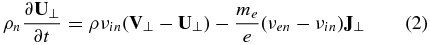
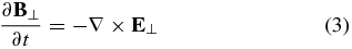

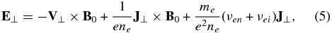
where  for the one-dimensional variation in the vertical direction, V⊥ and U⊥ are the horizontal bulk velocity of the plasma and neutral, respectively, E⊥, B⊥, and J⊥ are the horizontal electric field, (perturbation) magnetic field, and electric current density, respectively, ne is the electron number density, ρ and ρn are the plasma and neutral mass density, respectively, me is the electron mass, e is the elementary charge; νin, νen, and νei are the ion–neutral, electron–neutral and electron–ion collision frequencies, respectively, and μ0 is the permeability in a vacuum. The generalized Ohm's law is derived by combining the momentum equations of the electrons and ions, and neglecting the electron inertia, which is small on time scales longer than the electron plasma oscillation period, collision period, and electron gyroperiod (Rossi & Olbert 1970; Greene 1973; Song et al. 2005; Vasyliūnas & Song 2005). A charge quasi-neutrality has been assumed. Note that in vertical one-dimensional geometry, the horizontal forces associated with flow and pressure gradients are zero. The displacement current has been neglected because of non-relativistic motion associated with the waves of interest in the chromosphere.

Figure 1. (a) Density and temperature structures, adapted from the chromospheric model of Avrett & Loeser (2008). The transition region is located between about 2130 km and 2200 km. The lower ghost region is a linear extrapolation of the model to z = −600 km. In the upper ghost region, densities and temperature are set as uniform. (b) Altitude distribution of ion–neutral collision frequency νin, electron collision frequency νe = νen + νei, and neutral–ion collision frequency νni = ρνin/ρn. Ion and electron gyrofrequencies with an ambient magnetic field of 100 G are plotted as dashed and solid vertical lines, respectively. The parameters in the ghost regions are in dash-dotted lines.
Download figure:
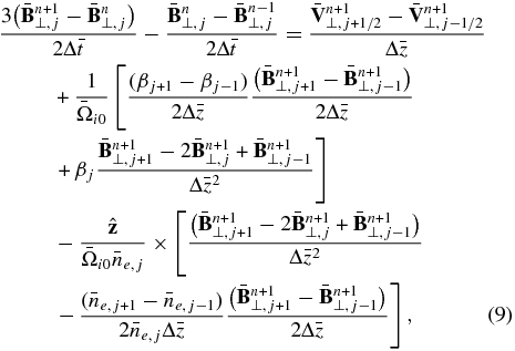
Standard image High-resolution imageThe mechanical energy input to the solar atmosphere is treated self-consistently to become wave energy with a part of it being dissipated into thermal energy by heating. Although energy equations are not included, if the thermal energy deposited is radiated, the present treatment remains self-consistent on the condition that the heat conduction is negligible. The heating rate (not temperature) can be evaluated based on the solutions of Equations (1)–(5). In a medium consisting of electron, ion, and neutral fluids, the total heating rate (plasma heating rate plus neutral heating rate) is represented by (Vasyliūnas & Song 2005)
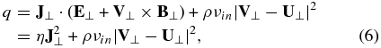
where η = me(νen + νei)/(e2ne) is the Ohmic resistivity. We have applied the generalized Ohm's law to obtain the second expression of Equation (6). The term J⊥ · (E⊥ + V⊥ × B⊥), associated with the electric field in the plasma frame of reference and determined by the last term of Equation (5), represents the true Joule heating, which is caused by electron collisions with other species. The term ρνin|V⊥ − U⊥|2 is the rate of frictional heating caused by collisions between ions and neutrals. On short time scales, the heat is deposited approximately equally to the plasma and neutral. On time scales much longer than the ion–neutral collision period, the heat is uniformly distributed in the whole medium and radiated.
By using Ampère's law to replace the current density in Equations (1), (2), and (5) and using the a generalized Ohm's law (5) to eliminate electric field in Faraday's law (3), we may obtain a set of equations for the plasma and neutral velocity V⊥ and U⊥, and perturbation magnetic field B⊥, which for the assumed one-dimensional geometry is perpendicular to the ambient magnetic field. This equation set describes the dynamics of the plasma, neutrals, and magnetic field on MHD time scales for the simple one-dimensional stratified solar atmosphere. A similar equation set has been obtained for the magnetosphere–ionosphere/thermosphere system and solved by a fully implicit difference method (Tu et al. 2011). Here we numerically solve the equation system using the fully implicit scheme, but with time difference given by a second-order backward difference formula (BDF2; Curtiss & Hirschfelder 1952). The resulting difference equations with normalized variables are
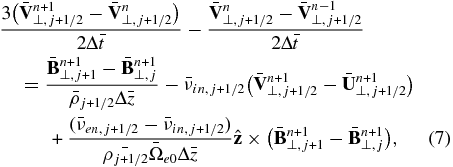
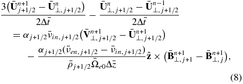
where the variables with a bar are normalized; superscripts n + 1, n, and n − 1 represent the (n + 1)th, nth, and (n − 1)th time step, respectively, and the subscript j is the spatial grid index;  and
and  are the normalized grid spacing and normalized time step, respectively;
  and
and  are the normalized electron and ion gyrofrequency, respectively, at the base of the nominal photosphere (i.e., at z = 0); α = ρi/ρn, and
 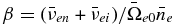 . The normalized variables are defined as
  ,
,  ,
,  ,
,  ,
,  ,
,  ,
,  ,
,  ,
,  ,
,  ,
,  , and
, and  , where ne0 and ρ0 are the electron density and plasma mass density, respectively, at z = 0,
  , and t0 = L/VA0 with L the length of the simulation domain. Note that t0 is dependent on the ambient magnetic field.
In Equations (7)–(9) the centered difference is used to represent spatial derivatives while the spatial grids are staggered: the plasma and neutral velocities are defined at j + 1/2 (i.e., at the middle of grids between j and j + 1) whereas the perturbation magnetic field is evaluated at the grid j. Numerical experiments show that the staggered grids help to avoid checkerboard numerical instability (Sigmund & Petersson 1998) in solutions in the region where there are large gradients in the velocity and/or perturbation of the magnetic field. The BDF2 time difference method with centered spatial difference results in second-order accuracy both in time and space difference. Note that in Equations (7) and (8) the centered difference is with reference to j + 1/2 so that the spatial differences involving grids j + 1 and j are second order in accuracy. The BDF2 time difference involves three levels of time steps: the current n + 1 and the two previous ones, n and n − 1. When n = 0 (at t = 0) the information before t = 0 is not available, so we use the standard backward time difference to get solutions at t = −Δt from given initial conditions at t = 0.
The implicit difference Equations (7)–(9) are a set of linear algebraic equations and are unconditionally stable so that the time step is not restricted by the Courant–Friedrichs–Lewy condition  , where
  is the normalized Alfvén speed. More importantly, due to very large collision frequencies (up to 1016 s−1) the momentum Equations (1) and (2) are strongly stiff. Therefore the collisional force terms dictate that a very small time step be required in order to obtain stable solutions if an explicit difference method is used. Test runs using an explicit backward Euler time difference showed that the time step must satisfy Δt < 10−8 s. Thereafter we use the real time unit to refer to time and time step since the normalized time and normalized time step are different for different ambient magnetic fields (due to different values of t0). The BDF2 time difference and implicit spatial difference overcome the stiffness so that the time step can be many orders of magnitude larger than that of explicit methods. The only constraint on the time step is the time resolution to resolve the physical processes of interest.
The solar atmosphere is assumed to be driven by a convective velocity at the nominal base of the photosphere, which is chosen as the origin of the z axis (z = 0). The semiempirical model of the quiet Sun atmosphere by Avrett & Loeser (2008) specifies the total hydrogen density, neutral hydrogen density, electron density, and solar atmosphere temperature from −100 km to about 68,000 km. We consider wave propagation from the assumed driving source (at the base of the photosphere, i.e., z = 0) to 3000 km, encompassing the transition region (between about 2130 km and 2200 km). In order to minimize the effects of artificial reflection at the boundaries of the simulation domain, we extend the simulation domain 600 km below z = 0 and 2000 km above z = 3000 km, i.e., there are two ghost regions. In the lower ghost region (from z = −600 km to z = 0 km) the neutral density and temperature below −100 km are linearly extrapolated. The ionization fraction is assumed to be constant in the lower ghost region although the results are not sensitive to the exact densities in that region as its function is to absorb the downward waves and to avoid reflection upward. In the upper ghost region (from z = 3000 km to z = 5000 km), however, the densities and temperature (thus collision frequencies) are uniform. Figure 1 displays the altitude distribution of the densities and temperature as well as the collision frequencies. The ion–neutral, electron–neutral, and electron–ion collision frequencies are calculated with the expressions given in De Pontieu et al. (2001), νin = 7.4 × 10⁻¹¹nnT1/2, νen = 1.95 × 10⁻¹⁰nnT1/2, and νei = 3.759 × 10⁻⁶neT−3/2, where the neutral and electron number density nn and ne are in cm−3, temperature T is in K, and ln Λ is the Coulomb logarithm.
In the panel showing collision frequencies, the ion and electron gyrofrequencies, Ωi and Ωe, for the ambient magnetic field B0 = 100 G are also plotted. The ion–neutral collision frequency is smaller than the ion gyrofrequency above about 800 km in this case so that at higher altitudes the ions become magnetized. The electron collision frequency (electron–neutral plus electron–ion) becomes less than the electron gyrofrequency at altitudes above about 100 km. Therefore, the Hall term in the generalized Ohm's law is larger than the resistive term in the high altitude chromosphere.
It is shown in the upper panel of Figure 1 that the densities in the lower ghost region increase with decreasing altitude. As a result, the propagation speed of the perturbations is very slow. The driving velocity is set at z = 0 in the simulations. Hence the time for the perturbations to travel back and forth between the driving source (z = 0) and lower boundary (z = −600 km) is over 18,000 s for the background magnetic fields considered, much longer than that in the region of interest (from 0 to 3000 km), even if the waves are not completely absorbed in the lower ghost region. For simplicity, we set lower boundary conditions as  ,
,  , and
, and  at z = −600 km.
For the upper boundary conditions, we note that the Alfvén waves are dispersionless and preserve the shape of the wave packets if the media is uniform, which is the case in the upper ghost region from 3000–5000 km. Therefore, non-reflecting boundary conditions can be achieved by setting  ,
,  , and
, and  , where
  is the normalized altitude of the top boundary (at 5000 km).
In the simulations we use a time step of Δt = 0.05 s so that the wave frequency up to 10 Hz can be sampled. Note that for a discrete time series, Nyquist frequency fN = 1/2Δt is the maximum frequency that can be resolved. We do not attempt to resolve higher frequencies by using smaller time steps because the waves with frequencies higher than 1 Hz carry little energy if the peak frequency of a power law spectrum is around 3 mHz.
The spatial grid spacing used is 0.25 km. Such small spacing is adequate for resolving short wavelength waves at low altitudes (below ∼100 km) where the Alfvén wave speed, calculated using the total mass density (the plasma plus the neutral ρt = ρ + ρn), can be as low as ∼0.3 km s−1, depending on the strength of the ambient magnetic field. For a 1 Hz wave, the wavelength is as short as about 0.3 km near the photosphere. The wavelength increases with altitude and becomes very large at high altitudes, up to 10,000 km. Although an efficient program should use non-uniform grid spacing with finer grids at lower altitudes (and the transition region) and coarser grid spacing at high altitudes, the non-uniform grid system, however, makes the difference equations more complicated and usually downgrades the accuracy of the spatial difference to the first order. For simplicity and accuracy, we choose uniform grids at the cost of efficiency.
Equations (7)–(9) are a system of linear algebraic equations, which can be cast concisely in the form of

where A is an N × N sparse matrix with N being the number of rows and columns, x the solution vector of N variables, and r a vector (N elements) as a function of solutions of the previous two time steps. There are many algorithms that have been developed to efficiently solve large linear equation systems with the sparse matrix, including those based on the Krylov subspace (KSP) method (e.g., Saad 2003). In the present study, we use a linear equation solver from the Portable Extensible Toolkit for Scientific Computation (PETSc) package developed by the PETSc team at Argonne National Laboratory (http://www.mcs.anl.gov/petsc). PETSc utilizes one of various KSP-based algorithms to solve a linear equation system either sequentially or in parallel (Balay et al. 1997). In the present simulations, the number of variables is very large: N = 6 × 22400 (and thus the number of matrix elements N2 ∼ 1.8 × 10¹⁰) but the number of nonzero elements is much smaller (∼8 × 10⁵). The PETSC solver handles the sparse matrix efficiently by storing only nonzero elements and the simulations based on this solver typically take about 160 minutes with the time step used, on a PC with an Intel core i-5 CPU and 8 GB RAM, to simulate wave propagation for a physical period of 16,000 s, which is the longest time period considered in the present simulations.
3. ALFVÉN WAVE PROPAGATION, REFLECTION, AND DAMPING
The simulations are conducted by using two types of driving velocity in the neutral velocity Ux component at the base of the photosphere (z = 0): either a rectangular pulse for examining the wave propagation and reflection or a broadband perturbation for studying the heating of the solar atmosphere.
3.1. Alfvén Wave Propagation and Reflection
We first examine the propagation and reflection of Alfvén waves by using the driving velocity of a rectangular pulse with a width in time of T = 80 s and neutral velocity Ux(z = 0) = 350 m s−1. The pulse rises to 350 m s−1 at t = 0 (without time delay) and falls to 0 m s−1 at t = 80 s. In this run we choose the ambient magnetic field B0 = 100 G. In Figure 2 we display altitude profiles of the magnitude of the plasma velocity, stacked in time with the time difference between the adjacent profiles being 40 s, to show the overall pulse evolution in space and time. From this z − t plot we can see that during the course of propagation the pulse experiences width broadening, amplitude change, and shape distortion. Initially the wave packet progressively moves upward with an increasing width. After the wave front reaches about 1500 km at about 440 s, the amplitude increases and the shape of the wave packet displays significant distortion. Later, the trailing edge starts to retreat because of the reflection. Thereafter a downward propagating wave packet is seen.

Figure 2. Altitude profiles of the magnitude of the plasma velocity stacked in time. The time separation of the profiles is 40 s. The ambient magnetic field B0 = 100 G.
Download figure:
Standard image High-resolution imageIn order to examine in detail the evolution of the wave packet, in Figure 3 we show altitude profiles of the x component of the plasma velocity, Vx, and the perturbation magnetic field, Bx, at four selected times. At t = 360 s the pulse reaches just below 500 km with its original rectangular shape preserved to a large degree. However, in the wake of the pulse, neither the velocity nor the perturbation magnetic field is zero (more clearly seen in panel (b)): there Bx has reversed the sign to positive (the same sign as that of Vx). This is a signature of reflected perturbations propagating downward (anti-parallel to the background magnetic field). Note that for Alfvén waves propagating parallel (anti-parallel) to the background magnetic field, the velocity and magnetic field perturbations are in the opposite (same) sign. At later times when the pulse has moved further upward, e.g., at 443 s shown in panel (b), the pulse is broader and its shape is distorted. The broadening is proportional to the Alfvén speeds between the pulse front and the trailing edge. Because the Alfvén speed increases with the altitude and the pulse width in time (T = 80 s) corresponding to a traveling distance, the pulse front propagates faster and faster than the trailing edge so that the pulse is progressively widened. The distortion of the pulse shape is caused by three effects. First, if there were no reflection and dissipation, required by conservation of the wave energy flux, the magnitude of the velocity would increase with altitude as (ρt, 0/ρt)1/4 and the magnitude of the perturbation magnetic field would decrease with altitude as (ρt/ρt, 0)1/4 (Song & Vasyliūnas 2013), where ρt, 0 is the total mass density at z = 0. Hence the velocity (magnetic field) amplitude within the pulse is larger (smaller) at increasing altitudes. Second, at each point the pulse is the superposition of the upward perturbation with that reflected from the parts in front. Since the velocity and perturbation magnetic field are in the opposite (same) sign for the Alfvén waves propagating parallel (anti-parallel) to the background magnetic field, the superposition of the upward and reflected perturbations enhances (reduces) the magnitude of the velocity (perturbation magnetic field). Such a change is more effective at lower altitudes of the pulse because there is greater reflection from the parts in front of it. Third, as will be shown in the next subsection, the waves of frequencies above a critical frequency fc (depending on the background magnetic field) are strongly damped. The pulse starts with a steep front which consists of perturbations of a broad frequency range (e.g., see panel (a)). The damping of the high-frequency waves makes the front less steep, i.e., the steep rising front becomes a gentle slope (e.g., panel (b)). The length of the slope is approximately given by VA, t/fc for the present case of B0 = 100 G, fc ∼ 0.12 Hz (see panel (c) of Figure 9). In panel (b) of Figure 3, the smoothed front slope starts from about z = 1000 km. Taking the value of VA, t = 41 km s−1 at 1000 km, the length of the slope is about 350 km, in agreement with that shown in panel (b) of Figure 3. When the front moves to even higher altitudes, because VA, t becomes very large, the front slope length is thus very long so that, essentially, the front is flattened out as demonstrated in panel (c). Further on in time, as shown in panel (d), having had experienced reflection and damping, the upward pulse has propagated outside the domain of interest, leaving a downward propagating reflected pulse. However, the perturbations in the wake of this reflected pulse are not zero (obviously non-zero Vx although Bx seems to be zero due to the scale of the y-axis). This is because the downward reflected pulse is also subjected to reflection and the re-reflected perturbations propagate upward.

Figure 3. Altitude variations of the x (horizontal) component of the plasma velocity (solid line) and perturbation magnetic field (dashed line) at four selected times. In each panel the scale for the velocity is on the left y-axis and the scale for the magnetic field is on the right y-axis.
Download figure:
Standard image High-resolution imageIn order to identify where the strongest reflection occurs, we compare, at given locations, Vx and  , which should be nearly the same in magnitude for Alfvénic perturbations, but opposite/identical in sign for purely upward (parallel to the ambient magnetic field)/downward (anti-parallel to the ambient magnetic field) propagation, based on the Walén relation
  if neglecting damping of the waves (e.g., De Pontieu et al. 2001; Song & Vasyliūnas 2011), where ∓ corresponds to the propagation parallel and anti-parallel to the ambient magnetic field, respectively. At the place of reflection (called local reflection) the magnitude of the velocity/perturbation magnetic field is either partially enhanced/reduced in the case of partial reflection or becomes doubled/zero in the case of total reflection. If the reflected pulse from the further ahead parts of the pulse is strong enough, it is possible for perturbation of the magnetic field to reverse the sign. Therefore, the relative difference between Vx and
  (or Vy and
  ) can be used to qualitatively determine the strength of the reflection.
In Figure 4 we display time variations of Vx and  at six altitudes. At low altitudes, like those shown in panel (a), we see that Vx and
  have nearly the same magnitude with an opposite sign for the upward pulse but with an identical sign for the reflected pulse. The front of the upward pulse arrives at 100 km at about t = 140 s and the trailing edge passes 100 km at about 220 s (80 s later). As shown in panel (a), after the trailing edge passed (i.e., after ∼220 s), Bx reverses the sign and Vx remains the same sign with a reduced (almost zero) amplitude, which are the perturbations reflected from the upward pulse that has moved above 100 km. It is seen that the magnitude of the reflected pulse increases with time, indicating that the reflection from higher altitudes becomes increasingly stronger (note that reflection from higher altitudes arrives at an observing location at a later time). The same feature of the reflection is seen at higher altitudes, say at 400 km (panel (b)). At higher altitudes, the reflected pulse comes back earlier because of the larger Alfvén speed. In addition, the original rectangular shape of the upward pulse is significantly distorted with Vx (
 ) increased (decreased), from the pulse front (earlier time) to the trailing edge (later time), in comparison to the original rectangular shape. Since the upward and reflected pulses are still separated in time, the deviation from nearly equal magnitude of Vx and
  must be primarily caused by local reflection. The stronger the local reflection is, the larger the ratio
  (or
(or  , not shown) is. Therefore, the waves experience partial reflection throughout the chromosphere with increasingly stronger reflection at higher altitudes.
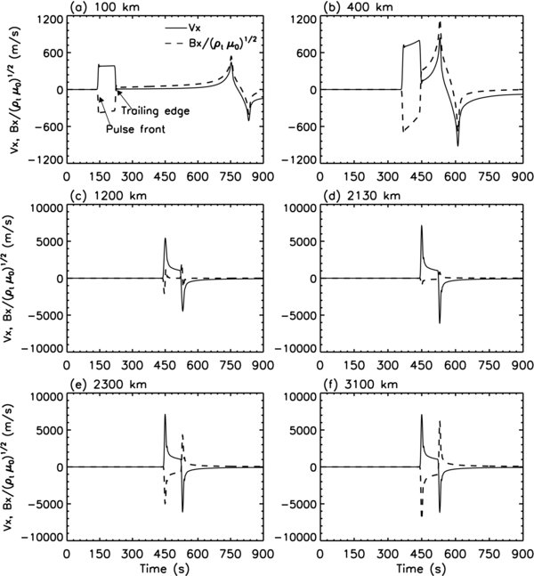
Figure 4. Time variations of Vx (solid lines) and  (dashed lines) at six selected altitudes. Panels (a) and (b) have different scales on their y-axes from those on the other four panels.
Download figure:
Standard image High-resolution imageThe increase of the ratio  is more evident at even higher altitudes. Panel (c) shows an example at 1200 km in which the reflected pulse almost completely overlaps with the upward pulse in time. The upward pulse (the velocity and perturbation magnetic field in opposite signs) can still be seen. At the front (earliest times) of the upward pulse the magnitude of
  is much smaller than that of Vx, indicating strong local reflection. Panel (d) displays the relation of Vx and
  at the lower edge of the transition region (at 2130 km), where the magnitude of
  at the pulse front is almost zero so that the ratio
  is larger than that observed at the pulse front in panel (c), implying stronger local reflection than that at 1200 km (panel (c)). Also noted is that the reflected pulse is no longer identifiable, indicating that the reflected pulse from the altitudes above is not strong enough to reverse the sign of the perturbation magnetic field. Indeed panel (e) shows that reduction in the magnitude of the perturbation magnetic field at the altitudes above the transition region is much weaker than that at 2130 km, indicating much weaker local reflection. Therefore, we can conclude that the strongest reflection occurs at the lower edge of the transition region.
The above conclusions are valid only if there is no contribution of the artificial reflection at the upper boundary (at 5000 km) of the simulation domain. We then examine the relation of Vx and  in the upper ghost region (see panel (f)) where the media is uniform and collisions are negligibly weak. We see that those two quantities are almost exactly the mirror image of each other, indicating the wave packet in the ghost region propagating purely upward. Particularly, this means no noticeable reflection from the upper boundary, an expected result from the non-reflecting boundary conditions discussed in Section 2. This is confirmed by checking the ratio of the plasma velocity to the perturbation magnetic field at the upper boundary, where we see an almost perfect Walén relation
  (data not shown), indicating nearly completely outgoing perturbations with negligible reflection at the upper boundary. Also note that the greater magnitudes of Vx and
  are due to the smaller density in the corona.
3.2. Chromospheric Heating
Having examined the Alfvén wave propagation and reflection in the above section, we now turn to calculating the rate of the chromospheric heating by the Alfvén waves. While a short pulse is better for illustrating the propagation and reflection, a continuously oscillating driving velocity is more suitable to examining wave heating. We thus conduct the simulations with a driving velocity Ux at z = 0 with a broadband time series specified by
where s and m are the number of frequencies (in logarithmic steps) below and above peak angular frequency ωp, respectively, Vb is an amplitude coefficient to make the time averaged energy flux, at z = 0,  erg cm−2 s−1, where VAt is the Alfvén speed at z = 0 calculated with the total mass density ρt and 〈〉 represents time average over the physical period simulated, and ϕk, ϕj = 2π rand()/(s + m) is the random phase with rand() being a random number taken from [0, s + m]. Note that only approximately half of the energy flux, or 107 erg cm−2 s−1, propagates upward and another half propagates downward into the lower ghost region. In the simulations we choose s = 10 and m = 590. The lowest and highest frequencies are f0 = ω0/2π = 1 mHz and fm = ωm/2π = 10 Hz, respectively, and fp = ωp/2π = 1.65 mHz.
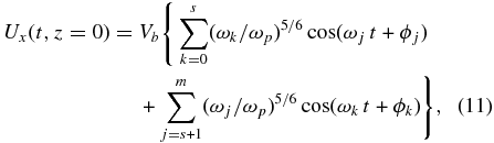
The simulated plasma and neutral velocities, and perturbation magnetic field are used to calculate the electric field and current via Equations (4) and (5). Then the heating rate can be evaluated with Equation (6). We consider four cases with different ambient magnetic fields: B0 = 10, 50, 100, 500 G. The time variations of Ux at z = 0 and associated energy flux spectra are shown in Figure 5 for the case of B0 = 50 G. The magnitude of the velocity is around 1 km s−1 with the peak at about 1.8 km s−1, within the range of the observed photospheric oscillation velocity (Avrett & Loeser 2008). The energy flux spectrum of the driving velocity is peaked at 3.3 mHz even though the spectrum of the driving velocity itself is peaked at fp = 1.65 mHz. This is because a Fourier transform of  produces doubled frequency components, which will be discussed in more detail later. The spectrum at frequencies higher than 3.3 mHz is close to a power spectrum with a power index of n = −5/3 (dashed line) while at frequencies lower than 3.3 mHz approximately follows a power law of a power index of n = 5/3.
Figure 5. Time variation (upper panel) of the driving velocity Ux at z = 0 for a broadband perturbation specified by Equation (11) for B0 = 50 G, and the corresponding energy flux spectrum (lower panel). The dashed line in the lower panel represents the power law variation (f/2fp)−5/3 for f > 2fp = 3.3 mHz and (f/2fp)5/3 for f < 2fp.
Download figure:
Standard image High-resolution imageFigure 6 shows the heating rate q as a function of time and altitude for the case of B0 = 50 G. Above the photosphere the heating rate is zero before the arrival of the perturbations from the source. The perturbation front reaches 3000 km at about 886 s in this case. It is seen that the heating is primarily at altitudes below about 800 km with the strongest heating below about 400 km, consistent with the result from the theoretical study of Song & Vasyliūnas (2011). Above the transition region the heating rate is more than 10 orders of magnitude smaller because of the negligibly small collision frequencies and the weaker available wave energy flux. Note that the present study does not invoke anomalous effects such as turbulence, which may produce higher heating rates in the corona. The local heating rate is about 0.1 erg cm−3 s−1 or larger at the lower chromosphere and above 10−2 erg cm−3 s−1 in the middle and high altitude chromosphere. Such values satisfy the heating rates required to balance the radiative energy loss in the quiet chromosphere (e.g., Withbroe & Noyes 1977; Vernazza et al. 1981). The heating rates show structures associated with the upward and reflected waves. The stronger (weaker) heating rates correspond to the larger (smaller) magnitude of the oscillating driving velocities shown in the upper panel of Figure 5.
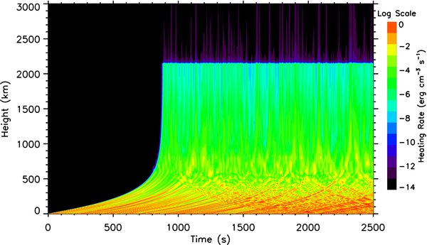
Figure 6. Variations of the heating rate with time and altitude. The ambient magnetic field is B0 = 50 G.
Download figure:
Standard image High-resolution imageAs indicated by Vasyliūnas & Song (2005), in partially ionized plasmas the heating is due to frictional dissipation caused by the ion–neutral collisions and Joule dissipation caused by the electron collisions with other species. In the case of the chromosphere, the Joule dissipation dominants the lower chromosphere because of large electron collision frequencies. This is confirmed by comparing the altitude distribution of the frictional and Joule heating rates shown in Figure 7. The heating rate at each altitude is averaged over the time period from the arrival of the perturbations to the end of the simulation (in this case 2500 s). It is seen that the frictional heating rate is much smaller than the Joule heating rate below about 600 km whereas the Joule heating rate is about 0.1 erg cm−3 s−1 or higher at low altitudes. The frictional heating becomes dominant only at higher altitudes but with a heating rate less than 10−3 erg cm−3 s−1. Therefore, if a heating mechanism, resulting from the collisional dissipation of the Alfvén waves in the chromosphere, operates primarily at high altitudes, like that of Leak et al. (2005), the derived heating rate would be considerably underestimated because the dominant heating in the region is only frictional heating, which is more than two orders of magnitude weaker than the Joule heating at the lower chromosphere.
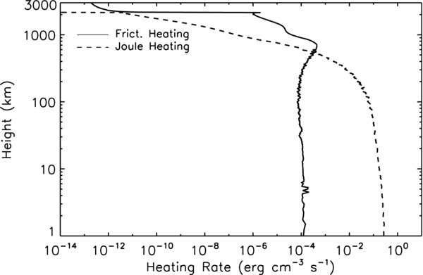
Figure 7. Altitude distribution of the time-averaged frictional (solid line) and Joule (dashed line) heating rates for the ambient magnetic field B0 = 50 G.
Download figure:
Standard image High-resolution imageFigure 8 displays the altitude distribution of the heating rate for B0 = 10, 50, 100, 500 G, averaged over the time in the same manner as in Figure 7. For the cases when the ambient magnetic field is less than 100 G, the heating rates in the lower chromosphere (below about 350 km) are ∼0.1 erg cm−3 s−1 or higher and then rapidly decreases with the altitude. The weaker the ambient magnetic field the larger the heating rate in the lower chromosphere (below about 500 km). At higher altitudes, however, the heating rate is larger for the stronger background magnetic field. This is because there is little wave energy left to heat the upper chromosphere due to strong wave damping for the weaker ambient magnetic field at low altitudes (Song & Vasyliūnas 2011).
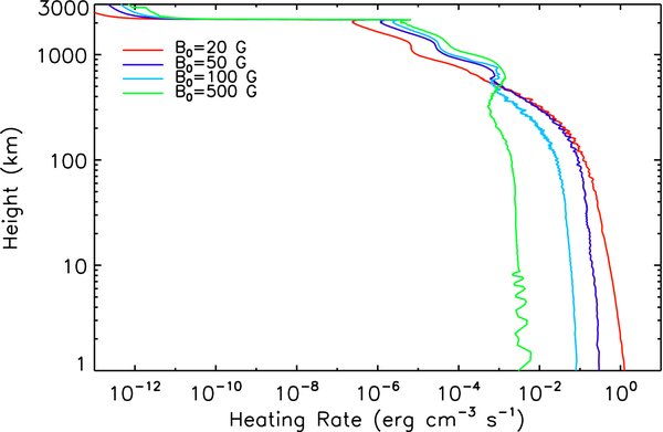
Figure 8. Altitude distribution of the time-averaged heating rate for the ambient magnetic field B0 = 10, 50, 100, and 500 G.
Download figure:
Standard image High-resolution imageFigure 9 displays spectra of the energy flux (Poynting flux Sz = E⊥ × B⊥/μ0) at 3100 km (in the upper ghost region) for the four different ambient magnetic fields. Here the energy flux spectrum is defined as the magnitude of a Fourier transform of Poynting flux. Note that there is essentially no reflection in the upper ghost region (including the top boundary) as shown in Section 3.1. Therefore, the energy flux at 3100 km represents that of the purely outgoing (transmitted) waves. The first feature we note is that each spectrum has an upper cutoff frequency because of the complete damping of the waves above that frequency. Specifically, the cutoff frequencies are about 0.014 Hz, 0.1 Hz, 0.4 Hz, and 0.7 Hz for B0 = 10, 50, 100, 500 G, respectively. Second, the remaining spectra deviate from a power law (power index −5/3, represented by dashed lines), starting from a frequency that depends on the ambient magnetic field, with progressively lower energy fluxes at higher frequencies compared to the dashed lines. This is caused by the strong but not total damping of the waves at those frequencies. This feature cannot be explained by simple reflection alone because the Alfvén waves are dispersionless so that the reflection should not be strongly dependent on frequency. The third feature is that compared to the energy flux density at the driving location (e.g., see panel (b) and lower panel of Figure 5), the energy flux density of the waves transmitted into the corona is one or more orders of magnitude lower because of wave damping and reflection. For B0 = 10 G, because most waves are damped before reaching the transition region, reflection is less important. The fourth feature is that for the stronger ambient magnetic fields the spectra are flatter at the low frequency end (but above fp). In these frequencies, damping is weak and reflection dominates at the transition region. In such cases, at any frequency, the perturbation is the superposition of the upward and reflected (and also re-reflected) waves. A Fourier transform of the energy flux at a given location consists of terms such as cos (ωt + ϕ1)cos (ωt + ϕ2), which leads to a component of doubled frequency even in a linear theory, where ϕ1 and ϕ2 are the phases of the upward and reflected waves at this height.

Figure 9. Energy flux spectra of waves transmitted to the corona (calculated at z = 3100 km; see text for details) for the ambient magnetic field B0 = 10, 50, 100, and 500 G. The dashed line in each panel represents the power law variation (f/fp)−5/3 for f > fp = 3.3 mHz and (f/fp)5/3 for f < fp.
Download figure:
Standard image High-resolution image
4. CONCLUSIONS AND DISCUSSION
In this study we present self-consistent solutions of plasma and neutral momentum equations and Maxwell's equations for a one-dimensional model of the chromosphere with incorporation of the Hall term, strong electron–neutral, electron–ion, and ion–neutral collisions. Treating the plasma and neutrals as two separate fluids allows us to explicitly calculate the frictional heating rate, which is shown to be much smaller than the Joule heating rate in the lower chromosphere. We simulate the propagation of a rectangular Alfvénic pulse from the base of the photosphere propagating to the corona. It is shown that the Alfvén waves are subject to diffused reflection throughout the chromosphere with increasingly stronger reflection at higher altitudes. The strongest reflection occurs at the transition region and the reflection in the corona is weak without considering anomalous effects such as turbulence and resonances. For a given wave packet, its width increases with the altitude because of the increasingly larger Alfvén speed at the front of the wave packet. The shape of the upward pulse is also distorted by the reflection and wave damping.
We apply broadband perturbations with a power law energy flux spectrum (power index close to −5/3, assuming that below the photosphere the flow is well-developed turbulence) as the photosphere driving source to evaluating the heating of the solar atmosphere by the Alfvén waves. It is found that the heating is concentrated below about 400 km. The Joule dissipation plays a dominant role in Alfvén wave heating of the chromosphere. The heating rate in the lower chromosphere is about 0.1 erg cm−3 s−1 or higher when the ambient magnetic field is weaker than 100 G, which is sufficient to balance the radiative loss in the lower chromosphere. At altitudes below about 500 km the weaker the ambient magnetic field B0 is, the stronger the heating is. At higher altitudes the reverse is true, but the height-integrated heating rate is always larger for the weaker background magnetic field. Waves above a certain frequency (depending on B0) are strongly damped and waves above a cutoff frequency (also dependent on B0) are even completely damped. The reflection also results in a frequency doubling effect that causes transfer of the energy from lower frequencies to higher ones so that wave damping (heating) is possibly stronger compared to that without reflection. Due to the reflection and strong damping, the wave energy flux transmitted to the corona is at least one order of magnitude smaller than that of the driving source. The Alfvén wave heating in the corona through inter-species collisional dissipation is negligible since the collisions in the corona are weak and the energy flux transmitted from the photosphere to the corona is small. Because the corona is nearly fully ionized, the radiation loss becomes small and the energy required for further temperature increase is also small.
The simulations show that if the convective flow at the base of the photosphere is large enough to carry the energy flux as observed, strong heating is possible, particularly in regions of weaker background magnetic fields. Previous theories and interpretation of observations may have overlooked the importance of the heating contribution from weaker field regions. One should not use the observed wave power to determine the heating rate because when the damping is high, the heating is strong and the observed wave power can be low.
In the present simulations we consider a simple one-dimensional geometry with spatial variation only along the vertical direction. With such a simple geometry we provide an essential description for the Alfvén wave propagation, reflection, and damping in the solar atmosphere. Particularly, we are able to unambiguously determine the wave reflection within the system by imposing two ghost regions and non-reflecting top boundary conditions to avoid the effects of artificial reflections from the simulation domain boundaries. The effects due to oblique propagation of the Alfvén waves are ignored and will be considered in the further development of our simulation model for two-dimensional/three-dimensional geometry. Nevertheless, we do not expect the results regarding the heating to significantly change in the case of oblique propagation because the group velocity of the Alfvén waves is always aligned with the magnetic field.
In the chromosphere above a certain altitude the Hall term is larger than the resistive term. While the Hall effect does not directly contribute to heating the chromosphere, it modifies the electric field and thus the perturbed magnetic field through Faraday's law. This in turn affects the plasma velocity through momentum Equation (1). Eventually, the heating in the chromosphere is modified by the Hall effect. Therefore, the Hall term must be retained to correctly account for the plasma (and also the neutral) dynamics as well as the heating of the chromosphere. This may be among the possible reasons why Leak et al. (2005) concluded that the heating is concentrated between 1000 km and 2000 km since the Hall term in their study was neglected.
The governing equations are strongly coupled through mutual collisions between the plasma and neutrals, particularly at low altitudes. This makes the equations strongly stiff which requires an implicit difference method to efficiently solve them. Otherwise very small time steps (<10−8 s) are required in order to obtain stable solutions if an explicit difference scheme is used. We have developed an implicit numerical framework that overcomes the stiffness and can use large time steps without losing the stability and accuracy. This implicit framework will allow us to develop efficient two-dimensional/three-dimensional models for modeling solar atmosphere dynamics.
This study was supported by the NSF grant AGS-0903777 and NASA grant NNX12AD22G to the University of Massachusetts Lowell.