


ABSTRACT
It is still a mystery how the solar chromosphere can stand high above the photosphere. The dominant portion of this layer must be dynamically supported, as is evident by the common occurrence of jets such as spicules and mottles in quiet regions, and fibrils and surges in active regions. Hence, revealing the driving mechanism of these chromospheric jets is crucial for our understanding of how the chromosphere itself exists. Here, we report our observational finding that fibrils in the superpenumbra of a sunspot are powered by sunspot oscillations. We find patterns of outward propagation that apparently originate from inside the sunspot, propagate like running penumbral waves, and develop into the fibrils. Redshift ridges seen in the time–distance plots of velocity often merge, forming a fork-like pattern. The predominant period of these shock waves increases, often jumping with distance, from 3 minutes to 10 minutes. This short-to-long period transition seems to result from the selective suppression of shocks by the falling material of their preceding shocks. Based on our results, we propose that the fibrils are driven by slow shock waves with long periods that are produced by the merging of shock waves with shorter periods propagating along the magnetic canopy.
Export citation and abstract BibTeX RIS
1. INTRODUCTION
The solar chromosphere is the layer of cool plasma (104 K) above the photosphere that sheds ultraviolet light and visible/near-infrared light at the wavelengths of strong spectral lines of neutral hydrogen, ionized calcium, ionized magnesium, and so on. The existence of the solar chromosphere has remained a mystery, since it stands much higher than can be supported against gravity by the force of the hydrostatic pressure gradient. The dominant portion of this layer must be dynamically supported, as is evident by the common occurrence of jet-like events. Once a jet is propelled, most of its material falls back to the photosphere, but some material can remain at high altitudes for a long time when it can be supported by a magnetic force. Some fraction of the jet material could be further heated and accelerated to become the origin of the solar corona and solar wind. Thus, revealing the driving mechanism of chromospheric jets has been one of the key problems in solar research.
What has fascinated solar scientists for a long time is that compressional waves propagating upward in a gravitationally stratified medium easily develop into shocks (Biermann 1948; Schwarzschild 1948) that can lift cool plasmas up (Parker 1964). This idea of shock driving was theoretically investigated in detail based on numerical simulations of spicules and mottles in quiet regions (Suematsu et al. 1982; Sterling & Hollweg 1988) and dynamic fibrils in active regions (Suematsu 1985; Sterling & Hollweg 1989), and is observationally supported by the pattern of motion detected in individual mottles (Suematsu et al. 1995) and dynamic fibrils (Hansteen et al. 2006; De Pontieu et al. 2007).
What then powers the shocks leading to chromospheric jets? Granular flows and global acoustic (p-mode) oscillations in the photosphere are obviously the most abundant energy sources in quiet regions. A significant amount of the energy of these motions can be transported upward by acoustic waves when the wave-guiding magnetic field lines are inclined from the vertical (De Pontieu et al. 2004). Apparently, this possibility is supported by the recent observational finding that dynamic fibrils of longer periods tend to be located in regions with more horizontal magnetic fields (Rouppe van der Voort & de la Cruz Rodriguez 2013). However, it should be noted that because of the strong magnetic field, photospheric motions inside sunspots may be much different from those of quiet regions.
The most well-known patterns of chromospheric motion inside sunspots are umbral oscillations and running penumbral waves. The physical nature of running penumbral waves has been controversial. Some (e.g., Tsiropoula et al. 2000) regarded them as trans-sunspot waves originating from umbral oscillations since they detected the waves starting from the umbra and propagating through the penumbra. Others (e.g., Christopoula et al. 2000; Kobanov et al. 2006; Jess et al. 2013) suggested that the waves are not real, but the visual pattern of upwardly propagating p-mode wave fronts along magnetic field lines of different inclination and different lengths. The picture of trans-sunspot waves assumes the existence of a driver localized somewhere near the axis of the sunspot, and the picture of upwardly propagating p-mode waves assumes the existence of large-scale coherent photospheric oscillations.
Here, we report our observational results indicating that chromospheric jets—specifically superpenumbral fibrils—outside of a sunspot, as well as penumbral waves, are closely related to the oscillations inside the sunspot. The results suggest that not only the umbral oscillations and the penumbral waves, but also the fibrils, may be powered by a common driver located at the axis of the sunspot below the surface.
2. OBSERVATION AND ANALYSIS
The region we observed (Figure 1) contains a few small sunspots of the same polarity without any penumbrae that are usually called pores. We inferred dynamical properties from high resolution spectrograms (Figure 2) taken with the Fast Imaging Solar Spectrograph (FISS) of the 1.6 m New Solar Telescope at the Big Bear Solar Observatory on 2013 July 17. The FISS is a dual-band Echélle spectrograph that can simultaneously take the Hα-band spectrogram and the Ca ii 854.2 nm band spectrogram using a single slit and two cameras (Chae et al. 2013). The integration time of each exposure was 30 milliseconds. The spectral sampling of the Hα spectrograms was 0.0019 nm, and that of the Ca ii spectrograms 0.0026 nm. Each Hα spectrogram covers 0.97 nm in the spectral domain, and each Ca ii spectrogram 1.3 nm. The spatial sampling along the slit was 0 16, corresponding to 116 km on the solar surface.

Figure 1. Upper left panel is the full-disk view of the solar photosphere taken at 19:30 UT in space by the Solar Dynamic Observatory, and the upper right is the close-up view of the rectangle area. The squares in these panels mark the 29,000 km by 29,000 km field of view of the Fast Imaging Solar Spectrograph (FISS) observation. The lower left shows the photosphere of the region observed by the FISS at 19:15 UT of 2013 July 17. The lower right panel is the magnetic map of the same rectangle area.
Download figure:
Standard image High-resolution image
Figure 2. Upper panels show examples of spectral images (spectrograms) of the slit taken at the Hα band and the Ca ii 854 nm band, respectively, and the lower panels show their contrast images normalized by the reference spectral profiles taken by averaging spectral profiles over the regions outside the sunspots. The dotted vertical lines refer to the wavelengths at which monochromatic images were constructed.
Download figure:
Standard image High-resolution imageThe raster scanning of the observing region is done using a linear-motorized scanner which moves the solar image across the slit step by step. The step size was set to the same value of the spatial sampling along the slit, 016. The quality of the imaging depends highly on that of the light fed into the slit, which is determined by the astronomical seeing and the performance of the adaptive optics (AO). Our observation was performed with 308 sub-aperture adaptive optics. We estimate that the spatial resolution of the raster images is around 035, which is about twice the pixel size. One raster scan consisting of 250 steps takes 35 s for completion and covers a field of view of 40'' by 40'', or 29,000 km by 29,000 km on the solar surface. The data obtained from each raster scan are used to construct monochromatic images at different wavelengths. The total number of raster scans in our observation was 75, which covers a period of 44 minutes starting from 18:50 UT of 2013 July 17. In summary, the data we used are four-dimensional (λ, y, x, t) arrays of Hα and Ca ii intensity data.
Our data analysis is aimed at revealing the spatiotemporal pattern of intensity and Doppler signal variations that is necessary for understanding the basic nature of oscillations and shock waves. Constructing the variation in intensity from the data is a trivial and straightforward task, but doing so for the Doppler signal is not. We choose the lambdameter method to construct the Doppler signal variations from the spectroscopic data. Figure 3 illustrates this method. The Doppler signal is determined from the center of the lambdameter, the chord of finite length—0.04 nm in the Hα line and 0.02 nm in the Ca ii line. The wavelength position and intensity level of the lambdameter are adjusted until it fits the line profile. We first calibrated wavelengths in the rest frame of the Earth making use of telluric absorption lines. Using this method, we infer the Doppler velocity of −2.4 km s−1 from the Hα line profile of interest, and that of 1.2 km s−1 from the Hα reference profile in the rest frame of the Earth (see the upper left panel of Figure 3); in the same way, we infer 0.0 km s−1 from the Ca ii line profile of interest, and +1.7 km s−1 from the Ca ii reference profile (see the upper right panel of Figure 3). If we change the rest frame to the reference profiles, which appears to be physically more meaningful than the rest frame of the Earth, then the Doppler velocity of the Hα line profile of interest becomes −4.6 km s−1 and that of the Ca ii line profile becomes –1.7 km s−1, both of which indicate upward-directed motions.
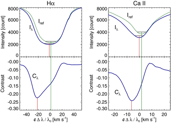
Figure 3. Illustrations of the determination of Doppler velocity using the lambdameter method (upper panels) and the maximum contrast method (lower panels) for the Hα line (left) and Ca ii line (right), respectively.
Download figure:
Standard image High-resolution imageThe lambdameter method is simple and works well without failure unless the line has an emission core, so it is very convenient for the study of the spatiotemporal pattern of the Doppler velocity. This method's main shortcoming is that the magnitude of the Doppler velocity is seriously underestimated compared with other methods (Chae 2014), due to the fact that the Doppler velocity is contributed to not only by the fast-moving chromosphere, but also by the slowly moving photosphere. Despite this shortcoming, the Doppler velocities determined with this method are still useful for the investigation of the spatiotemporal pattern of the Doppler velocity since they are strongly correlated with those determined using other methods (Chae 2014).
When a better estimate of the specific velocity values is necessary, we have to rely on other methods. The lower panels of Figure 3 show that the chromospheric contribution to the Doppler velocity is better inferred from the analysis of the contrast profile defined as Cλ = (Iλ − Iref)/Iref. Here, Iλ refers to the line profile of interest, and Iref refers to the reference profile. Given the line profile of interest Iλ at a spatial point, we construct its reference profile Iref by taking an appropriate average of all the profiles taken at different times at the same position. At every wavelength position, we take the average of the top 30% of intensity values to minimize the effect of the absorption features themselves on the reference profile. As another measure of Doppler velocity of the chromospheric plasma, we choose the wavelengths where the contrast is the highest (darkest). In the rest frame of the average chromosphere, the Doppler velocity determined using this maximum contrast method is found to be −23.5 km s−1 in the Hα line (see the lower left panel of Figure 3), and −8.1 km s−1 in the Ca ii line (see the lower right panel of Figure 3), the magnitudes of which are much larger than those determined using the lambdameter method. We also find that there is a systematic difference in the magnitude of the Doppler velocity between the Hα line and the Ca ii lines, which may be because the Ca ii line is formed at lower heights of higher mass density than the Hα line.
3. RESULTS
3.1. Patterns of Oscillations and Outward Propagation
Monochromatic images (Figure 4) constructed from the spectrograms indicate that the major component of the chromosphere of the observed region seen through the Hα and Ca ii lines is the fibrils—thin and long dark features—that emanate from the area surrounding the sunspot area and are radially extended. These fibrils form the superpenumbra of the sunspot, which has no penumbrae. These superpenumbral fibrils vary greatly with time, displaying complex motion and brightness variability (see Figure 5 and the accompanying movies). The most dynamic among these fibrils are those that are to the west of the largest sunspot (as traced by curve A in the figures).
Download figure:
Video Standard image High-resolution imageDownload figure:
Video Standard image High-resolution imageDownload figure:
Video Standard image High-resolution imageDownload figure:
Video Standard image High-resolution imageDownload figure:
Video Standard image High-resolution imageFigure 4. Monochromatic images of the observed region constructed at the different wavelengths of the Hα band (reddish color) and the Ca ii band (greenish color) from the same raster scan made at t = 22.15 minutes. The fibrils in path A are more dynamic than those in path B. The time variation of the features at different wavelengths can be seen from the corresponding movies.
(Animations (4a, 4b, 4c, 4d, 4e and 4f) and a color version of this figure are available in the online journal.)
Download figure:
Video Standard image High-resolution imageFigure 5. Dopplergrams constructed at t = 22.15 minutes using the lambdameter method. The time variation of the Doppler signal can be seen from the corresponding movie.
(An animation and a color version of this figure are available in the online journal.)
Download figure:
Video Standard image High-resolution imageThe movies—particularly those of the blue wing intensity and Doppler velocity—qualitatively show that the fibrils are closely related to the oscillations inside the sunspot. We find oscillations of both the intensity and Doppler velocity inside the sunspot, which correspond to well-known umbral oscillations, and outward-propagating patterns of intensity and Doppler velocity outside the sunspot. These patterns look similar to the running penumbral waves seen in the sunspot penumbrae, even though our sunspot does not have any penumbrae. They often propagate far until they reach the fibrils. The physical connection between the umbral oscillations and the fibrils is thus established through these propagating patterns.
The temporal-spectral variations (t–λ plots) of the intensity contrast (Figure 6) indicate that the oscillations at every position on the path connecting the sunspot to the fibrils are in fact upwardly propagating shock waves. The passage of an upwardly propagating shock through the chromosphere produces the sawtooth or N-shape pattern of the absorption core in this plot, which characterizes the sudden appearance of a large blueshift (compression phase or the shock front itself) followed by the gradual drift to large redshift (expansion phase, "post-shock" flow), and the next sudden appearance of a large blueshift (Hansteen et al. 2006; Vecchio et al. 2009). The N-shape pattern prevails in all of the t–λ plots constructed at six different locations, and hence confirms the idea of shock-driven fibrils. The amplitude of the Doppler velocity fluctuations (velocity jump in the shock front) inferred from the maximum contrast wavelengths ranges from 40 to 50 km s−1 in the Hα line and from 20 to 25 km s−1 in the Ca ii line.
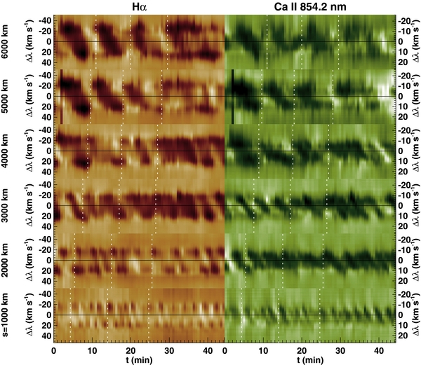
Figure 6. Time–wavelength maps (t–λ plots) of the intensity contrast at six different locations (labeled by distance s) along path A. The intensity contrast is defined by the ratio of the intensity difference to the reference intensity, which is taken from the temporal average. The dotted vertical lines refer to the times of the long-distance, outward-propagating patterns at each position.
Download figure:
Standard image High-resolution imageThe patterns of oscillations and outward propagations can be investigated in detail with the time–distance maps (t–s plots) of the intensities and Doppler velocities (Figure 7). The oblique patterns of intensity and Doppler velocity seen in these maps are quite consistent with the notion of outward-propagating patterns. Of particular interest to us is the existence of long-distance outward-propagating patterns (marked by the dotted curves on the maps) that start from the center of the sunspot, propagate like running penumbral waves, and reach the dynamic fibrils further apart. We have determined these patterns by identifying the times of the sudden appearance of upward motion—which is an indication of a upwardly propagating shock front—as functions of distance. Since the sudden appearance of upward motion corresponds to the front of an upwardly propagating shock wave, each curve in the maps of Figure 7 represents the trajectory of an outward-propagating pattern of upwardly propagating shock fronts. The sudden-appearance time of upward motion at each height is basically identified either from the boundaries of the absorption structures seen in the maps of blue wing intensity or from those of the blueshift ridges seen in the maps of Doppler velocity.
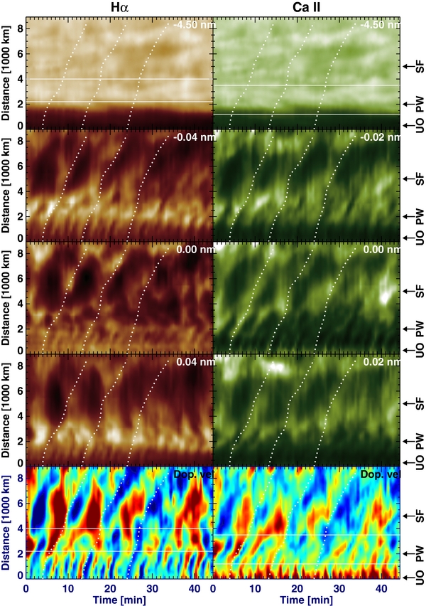
Figure 7. Time–distance maps or t–s plots of intensities and Doppler velocity constructed along curve A in the Hα line (left) and the Ca ii line (right). The arrows on the right side mark the regions of umbral oscillations (UO), penumbral waves (PW), and superpenumbral fibrils (SF). The dotted curves refer to the trajectories of the long-distance, outward-propagating pattern of shock fronts. The horizontal lines refer to the heights of the oscillation jumps. The blue and red colors at the bottom of the maps represent Doppler velocities of −2.5 km s−1 (blueshift, upward motion) and +2.5 km s−1 (redshift, downward motion), respectively.
Download figure:
Standard image High-resolution imageThe slope of a curve in the t–s plots (Figure 7) corresponds to the plane-of-sky propagation speed of the corresponding shock front. We find that the average speed is 14 km s−1, but in fact it varies significantly with position, being larger than 20 km s−1 inside the sunspot, decreasing to a value as low as 7 km s−1 outside the sunspot, increasing to a peak value higher than 40 km s−1 in the lower parts of the fibrils, and then decreasing again back to a low value of about 10 km s−1 in the upper parts of the fibrils.
The t–s maps of Doppler velocity in Figure 7 also indicate that the consequent redshift ridges often merge, forming the pattern of forks in the t–s maps. This merging occurs when the following ridge has a larger slope than the preceding one—which means faster propagation—or a negative slope—which means inward propagation. Blueshift ridges often disappear when they are enclosed by the fork pattern of the redshift ridges.
Our data suggest that in addition to the dynamic fibrils, other relatively stable fibrils are driven in close association with the sunspot oscillations. The fibrils occurring along path B (Figure 4) illustrate such fibrils. From the time–distance maps of intensity (see Figure 8), we find that the lifetime of a fibril in this region is as long as half an hour, during which the fibril was propelled by shocks several times, in contrast to the dynamic fibrils described above, each of which was propelled by a single shock. Despite this minor difference, the major conclusions made for the dynamic fibrils also hold in the case of the stable fibrils: the shocks driving the fibrils are related to the sunspot oscillations. In other words, there exist propagating patterns of shock wave fronts that start from the sunspot center and reach the bottoms of the fibrils. It is thus clear that both the dynamic fibrils in path A and the stable fibrils in path B are physically related to the oscillations of the sunspot, and the pattern of shock fronts propagates isotropically from the center of the sunspot.

Figure 8. Time–distance maps of intensity and Doppler velocity constructed along path B.
Download figure:
Standard image High-resolution image3.2. Short-to-long Period Transition and Shock Wave Interaction
Our next finding is that the predominant period changes as the waves propagate. Figure 6 clearly shows that the successive arrival of shocks at a fixed position is responsible for the previously reported oscillations in monochromatic intensity and velocity in the chromospheric network (Lite et al. 1993), mottles (Tziotziou et al. 2004), and fibrils (De Pontieu et al. 2003). The figure, moreover, indicates that the pattern of shocks progressively changes with distance: shocks come in fast cadence in regions close to the origin, and in slow cadence in regions further away from it, which suggests the short-to-long period variation. This period variation is clear in the time variations of the Doppler velocity shown at several different locations (Figure 9). The plot of predominant period versus distance indicates that the period changes from about 3 minutes near the origin (in the sunspot) to about 10 minutes at long distances (in the dynamic fibrils). Since a similar short-to-long period variation was recently reported in another sunspot (Maurya et al. 2013), this behavior seems to be a general property of sunspots in the chromosphere.

Figure 9. Plots of Doppler velocity versus time at three selected locations, and a plot of the predominant period versus distance. The red curves are from the Hα line, and the blue ones are from the Ca ii line.
Download figure:
Standard image High-resolution imageHow does this short-to-long period variation occur? We have obtained results suggesting that it may result from the non-linear interaction of shock waves. First, we find that the variation of period over distance is not smooth, but is often discontinuous. Figure 9 shows that in the Hα line, the period jumps from 3 minutes to 4.5 minutes at a distance of 2200 km, and from 6 minutes to 8.5 minutes at a distance of 4000 km. In the Ca ii line, the period jumps from 2.7 minutes to 3.6 minutes at a distance of 1200 km, and from 5 minutes to 8.5 minutes at a distance of 3500 km. The range of distance from 3500 to 4000 km where major period jumps occur corresponds to the region where the footpoints of the fibrils are located. As mentioned above, we also found the fork patterns of the redshift ridges, indicating the merging of the redshift ridges and the suppression of the blueshift ridges. Figure 7 shows that the period jumps preferentially occur at the heights where the fork patterns of redshift ridges develop.
The time series of the spectral–spatial (λ–s) plots in Figure 10 shows the events resulting from the interaction of shocks. One kind of events is shock merging. Note that in a λ–s plot, a shock front and its post-shock flow appear as a single continuous pattern of shock flow with the front moving upward (characterized by Doppler velocity <0 and vertical velocity v > 0) and the rear moving downward (Doppler velocity >0 and v < 0). When the rear of the preceding shock flow comes close to the front of the following shock flow, both the downward moving plasma and the upward moving plasma may be located inside the spectral line forming the volume along the same line of sight. The observable consequence is the occurrence of two Doppler components in the same contrast profile: a blueshifted component and a redshifted component. As a matter of fact, we can find from Figures 6 and 10 specific distances and specific times where the contrast profile displays two distinct components. A similar behavior was recently found from IRIS observations in the Si iv 139.3 nm line as well (Tian et al. 2014). We also find that at some instants, the front of the following shock flow switches from upward motion to downward motion. As a result, the two shock flows merge and become a single continuous flow predominantly moving downward (see the Ca ii λ–s plot at t = 15.6 minutes). This process of shock merging is consistent with the merging of redshift ridges mentioned above. The other event associated with shock interaction is the brightenings seen in the cores of the lines, particularly in the Ca ii line, as indicated by the black arrows in the figure. These brightenings may be considered as evidence of enhanced heating resulting from the interaction of shocks.
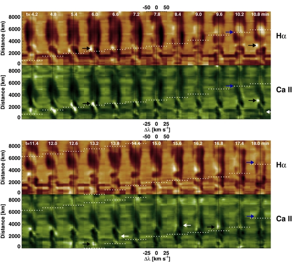
Figure 10. Time series of wavelength–distance (λ–s) plots of intensity contrast (top: Hα, bottom: Ca ii) along path A. The dotted horizontal lines refer to the positions of the propagating wave fronts at each time. The white arrows mark the events of shock merging, the black ones mark the brightenings associated with the shock interaction, and the blue ones mark the propelling of the fibrils.
Download figure:
Standard image High-resolution imageWe propose that the non-linear interaction of shock waves can lead to the short-to-long period transition. To illustrate the non-linear interaction of shock waves, let us consider a simple model of non-linear longitudinal waves where the phase speed cp of a pattern is given by the zero-velocity phase speed, c, plus the plasma velocity, v, that is, cp = c + v. What is important here is that the front of a wave with v > 0 and the rear with v < 0 propagate at different speeds. As the amplitude of the velocity increases, the front propagates upward faster and faster, but the rear propagates slower and slower, and may even reverse its propagation direction. This non-linearity partly explains the difference in shape and slope between the redshift ridges and the blueshift ridges in the t–s plot of the Doppler velocity (Figure 7). The difference in the propagation speed between the front of a shock wave and the rear of the preceding post-shock flow causes them to collide. What will result from this collision? If the front of a shock is overwhelmed by the rear of its preceding shock, then the direction of plasma motion will change from upward to downward and its identity as a shock will be entirely lost. The consequences of this will be the appearance of a merged shock with a lengthened rear part (as marked by the white arrows in Figure 10, the merging of the redshift ridges in the t–s plot of Doppler velocity (Figure 7), and the sudden increase of period with distance (Figure 9). It is likely that the energy of the colliding shocks may partly dissipate into heat and partly accumulate in the volume where the collision preferentially occurs. The brightening seen in the core of the Ca ii line (marked by the black arrows in Figure 10) may be considered as evidence for the enhanced heating resulting from such a collision.
4. DISCUSSION
We have obtained observational results that are helpful in revealing the relationship among umbral oscillations inside the main sunspot, running penumbral waves just outside it, and fibrils in its superpenumbra. One basic result is that at every position in these features, the t–λ plots displays a sequence of N-shaped patterns that are compatible with the passage of a train of upwardly propagating shock waves, which confirms the findings of previous studies (Hansteen et al. 2006; De Pontieu et al. 2007; Rouppe van der Voort & de la Cruz Rodriguez 2013). Recent 01 resolution observations revealed that the shock waves in the sunspot umbra appear as short and very thin chromospheric jets called umbral spikes (Yurchyshyn et al. 2014). A more important finding is the horizontally propagating patterns of shock fronts seen in the t–s plots of velocity that apparently originate from inside the sunspot, propagate outward as running penumbral waves, and develop into fibrils. This finding is compatible with previous reports of patterns connecting between umbral oscillations and penumbral waves (Alissandrakis et al. 1992; Tsiropoula et al. 2000). The connection between the sunspot and the fibrils, however, has not been reported previously. We also found that the period of oscillation increases with distance from the sunspot. The center of the sunspot displays the well-known 3 minute oscillations while the fibrils oscillate with much longer periods of about 10 minutes. This also confirms the previous studies of Tziotziou et al. (2006, 2007), Rouppe van der Voort & de la Cruz Rodriguez (2013), and Jess et al. (2013). The increase in the period often occurs discontinuously at some distances, which is also consistent with the previous studies of Tziotziou et al. (2006, 2007).
The most interesting finding of our study is the propagating patterns of velocity interacting with each other. Redshift ridges often merge to form the fork patterns, and blueshift ridges are suppressed by such merging. We can identify the fork pattern of redshift ridges even in the previously reported time–distance plots of the Doppler velocity—e.g., Figure 2 of Tziotziou et al. (2006), Figure 6 of Maurya et al. (2013), and Figure 2 of Tian et al. (2014)—even though none of these previous studies explicitly reported this finding. We interpret the fork pattern of the redshift ridges as the merging of shocks resulting from the suppression of a shock that occurs when the front of a shock meets with its preceding post-shock flow. The merging of shocks leads to the increase of the arrival time interval of subsequent shocks, providing a physical explanation of the observed short-to-long period transition.
Our results lead us to conclude that the pattern of outward propagation inside the sunspot is not real, but apparent. Since our results confirm that the oscillations inside the sunspot represent upwardly propagating shock waves, and the magnetic field lines are predominantly vertical inside the sunspot, the real direction of shock propagation should be along magnetic field lines, and the trans-sunspot picture turns out to be invalid. The apparent outward propagation should be explained by the proposed visual pattern of upwardly propagating slow shock waves along magnetic field lines of different inclination and different path lengths. The short-to-long period transition inside the sunspot can be explained by this scenario since the acoustic cutoff period increases with field inclination.
We think, however, that the pattern of outward propagation outside the sunspot may be real because the observed merging of redshift ridges is difficult to explain with the visual pattern of upwardly propagating shocks along different field lines. As an alternative, we propose the pattern of outward propagation outside the sunspot represents the slow shock waves propagating along the highly inclined field lines that form the canopy structure. Slow shock waves propagating along such field lines can display both the pattern of outward propagation and the signature of upwardly propagating shock waves. Since the slow shock waves are longitudinal, they can interact with each other to merge during the propagation, as suggested by our observations.
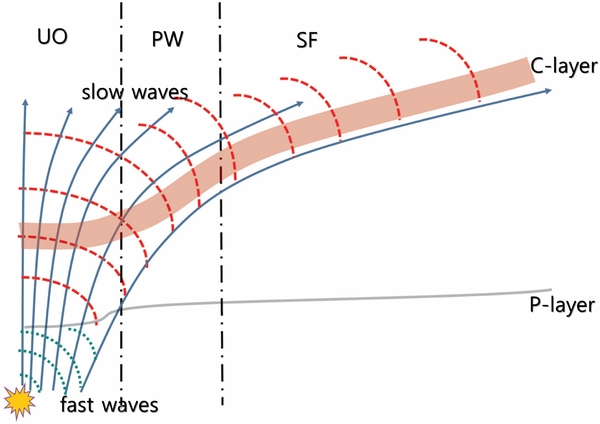
The observed close relationship between the umbral oscillations, the penumbral waves, and the fibrils suggests that these events should have a common origin. Figure 11 presents our picture of these related events. We conjecture that the sunspot is somehow excited below the surface. As a matter of fact, the numerical experiment of Felipe et al. (2010) demonstrated that all of the slow magneto-acoustic waves in the atmosphere of a sunspot can originate from a single driver localized on the axis of the sunspot below the layer where the Alfvén speed vA equals the sound speed cS. It was found that the energy of excitation is first transported across the field lines in the form of fast magneto-acoustic waves below vA = cS, and when these fast waves reach the surface of vA = cS, they are continuously transformed into slow magneto-acoustic waves that follow different field lines.
Figure 11. Unified picture of umbral oscillations (UO), penumbral waves (PW), and superpenumbral fibrils (SF) driven by an exciting source located on the axis of the sunspot below the surface, the P-layer. These events are different manifestations of slow magneto-acoustic shock waves occurring in the C-layer where the cores of the Hα line and Ca ii 854.2 nm line are formed.
Download figure:
Standard image High-resolution image
Only those components with frequencies higher than the cutoff frequency propagate upward to develop into slow shock waves. Inside the sunspot, the upwardly propagating slow shock waves along different field lines of different inclination produce umbral oscillations, penumbral waves, and the visual pattern of outward propagation. Outside the sunspot, however, the slow shock waves propagating along the inclined field lines of the canopy structure produce the real pattern of outward propagation. These shock waves interact with each other during propagation, often merging each other and producing shock waves of long periods. It is these slow shock waves of long periods that may drive the fibrils.
We are grateful to the referee for critical comments which helped significantly to improve our manuscript. This work was supported by the National Research Foundation of Korea (NRF-2012R1A2A1A03670387). Vasyl Yurchysyn's effort was supported by NASA grants LWS NNX11AO73G and NSF AGS-1146896. K.S.C. was supported by the Development of Korea Space Weather Center of KASI and the KASI basic research funds.