


ABSTRACT
Solar flares produce non-thermal electrons with energies up to tens of MeVs. To understand the origin of energetic electrons, coronal hard X-ray (HXR) sources, in particular above-the-looptop sources, have been studied extensively. However, it still remains unclear how energies are partitioned between thermal and non-thermal electrons within the above-the-looptop source. Here we show that the kappa distribution, when compared to conventional spectral models, can better characterize the above-the-looptop HXRs (≳15 keV) observed in four different cases. The widely used conventional model (i.e., the combined thermal plus power-law distribution) can also fit the data, but it returns unreasonable parameter values due to a non-physical sharp lower-energy cutoff Ec. In two cases, extreme-ultraviolet data were available from SDO/AIA and the kappa distribution was still consistent with the analysis of differential emission measure. Based on the kappa distribution model, we found that the 2012 July 19 flare showed the largest non-thermal fraction of electron energies about 50%, suggesting equipartition of energies. Considering the results of particle-in-cell simulations, as well as density estimates of the four cases studied, we propose a scenario in which electron acceleration is achieved primarily by collisionless magnetic reconnection, but the electron energy partition in the above-the-looptop source depends on the source density. In low-density above-the-looptop regions (few times 109 cm−3), the enhanced non-thermal tail can remain and a prominent HXR source is created, whereas in higher-densities (>1010 cm−3), the non-thermal tail is suppressed or thermalized by Coulomb collisions.
Export citation and abstract BibTeX RIS
1. INTRODUCTION
A solar flare is an explosive energy-release phenomenon on the Sun that accelerates a large number of electrons up to tens of MeV (e.g., Frost 1969; Lin & Hudson 1976). To diagnose these accelerated electrons, hard X-ray (HXR) observations of electron bremsstrahlung emission have been used (e.g., Brown 1971). In general a relatively high energy (typically ≳15 keV) HXR emission comes from chromospheric footpoints of a flaring loop, which is also visible in soft X-ray or extreme-ultraviolet (EUV) images. Conversely a relatively low energy (typically ≲15 keV) HXR emission comes from the apex of the flaring loop or looptop.
In some cases, the higher energy (≳15 keV) HXRs can be detected not only at the footpoints but also in the corona. The source can be located slightly above the brightest looptop region, and such a location suggests that magnetic reconnection in a coronal current sheet plays a role for producing energetic electrons (Masuda et al. 1994). Unfortunately, the possible reconnection region in the corona does not produce a detectable amount of HXRs, which is probably because of the rather low coronal density. Hence, the above-the-looptop source has remained an important observational target for obtaining a clue to the origin of energetic electrons (e.g., Tomczak 2001; Petrosian et al. 2002).
However, it is still unclear how energies are partitioned between thermal and non-thermal electrons within the above-the-looptop source. An earlier study of the Yohkoh data with four energy bands in the HXR range suggested the presence of a very hot (∼100 MK) thermal plasma in such a source (Masuda et al. 2000). A more recent mission, the Reuven Ramaty High Energy Solar Spectroscopic Imager (RHESSI; Lin et al. 2002), provides data with higher spectral resolution, which allows us to examine the energy partition in a greater detail.
A caveat is that the looptop source is so bright that it generally masks the above-the-looptop spectrum in the lower-energy (<15 keV) range for RHESSI. In a statistical analysis of the combined (i.e., looptop and above-the-looptop) coronal spectrum, Krucker & Lin (2008) established the existence of two distinct spectral components: an intense thermal component dominant in the lower energy range and a secondary component in the higher energy range that shows time variations much faster than those of the intense thermal component.
In SOL2007-12-31, the higher-energy component of the coronal spectrum was clearly non-thermal. By applying a power-law to the higher energy component of the combined coronal spectrum, it was argued that all electrons are accelerated (Krucker et al. 2010). For a more recent flare, it was argued that the ratio of thermal proton density to non-thermal flare-accelerated electron density was of order unity (Krucker & Battaglia 2014).
In contrast, detailed studies of spatially integrated spectra (i.e., without separating chromospheric footpoint sources, let alone the coronal looptop and above-the-looptop sources) have sometimes suggested a superhot (≳30 MK) thermal source in addition to the hot (≲30 MK) looptop source (Longcope et al. 2010; Caspi & Lin 2010). Such an interpretation suggests very small non-thermal fractions of electron number and energy densities.
Recently, Oka et al. (2013) considered the possibility of having both superhot-thermal and non-thermal components within the above-the-looptop source. They showed that the higher-energy component of the combined coronal spectrum obtained on 2007 December 31 can be represented not only by the power law but also the kappa distribution model, as well as the combined model of thermal Maxwellian plus power-law distributions. By taking the difference between the fitted kappa distribution and its thermal core, they suggested a super-hot temperature ∼28 MK with fairly large non-thermal fractions of electron number density ∼20% and energy density ∼52% for the above-the-looptop source. Note again that the above-the-looptop source can be analyzed only in a limited energy range (typically 15–80 keV) so that a variety of different spectral models can fit the data.
In this paper, we extend the work of Oka et al. (2013). We studied four different above-the-looptop sources, which allowed us to examine the generality of both "thermal+power-law" and "kappa" models. We mainly use the X-ray data obtained by RHESSI. When available, we also use the EUV data obtained by the Atmospheric Imaging Assembly (AIA) on board the Solar Dynamic Observatory (SDO) to constrain the low energy end of the distribution.
The paper is organized as follows. In Section 2, we describe spectral models used in the analysis. In Section 3, we present a detailed analysis of the four above-the-looptop sources. We will describe SOL2012-07-19 in detail because it clearly showed a non-thermal component and the EUV measurement allowed us to study a lower energy range. We will discuss results in Section 4 and conclude in Section 5.
2. MODELS OF ENERGY SPECTRUM
Figure 1 illustrates the spectral forms considered in this paper to represent the energy spectrum of the above-the-looptop source. The thermal (Figure 1(a)) and power-law (Figure 1(e)) models are the extreme cases, with 0% and 100% non-thermal fractions, respectively. For the thermal model, the density distribution (cm−3 keV−1) can be written as
where E is the particle energy, NM is the number density, and TM is the Maxwellian temperature. For the power-law model, the density distribution (cm−3 keV−1) can be written as

where NPL is the number density, Ec is the lower-energy cutoff and δ is the power-law index.
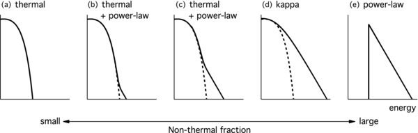
Figure 1. Schematic illustration of previously proposed spectral models of the above-the-looptop source. The distributions represent a plasma population in the above-the-looptop source alone. The vertical and horizontal axes represent differential density F(E) and electron energy E, respectively, in logarithmic scale. The models are shown, from left to right, in order of increasing magnitude of non-thermal, power-law component with a fixed spectral slope. Panel (d) may be regarded as the case of a saturated non-thermal tail. We consider that such a distribution can be represented by the kappa distribution. Here, the core distributions (dashed curves) are adjusted as described in the text. Panel (e) is an oversimplified version of non-thermal distribution without a core.
Download figure:
Standard image High-resolution imageThe combination of the two distributions (i.e., thermal+ power law; Figures 1(b) and (c)), is more generic and may be applied in many cases of spectral analysis. Note again that we are considering above-the-looptop sources only and the thermal distribution considered in this figure should not be confused with the thermal distribution in the brightest looptop region. Note also that the thermal+power-law model illustrated in Figures 1 (b) and (c) is conceptually the same as the hybrid thermal/nonthermal model considered by Holman & Benka (1992). A difference is that they applied the model to what we now regard as the spatially integrated spectrum of both coronal and footpoint sources, whereas we focus only on the above-the-looptop source. Moreover, they interpreted the lower-energy cutoff Ec as the critical energy above which runaway acceleration occurs.
In Figure 1 the thermal core distribution (density NM and temperature TM) and the power-law spectral index γ are fixed. The intensity of the power-law component is larger in Figure 1(c) than that in Figure 1(b). The intensity of the power-law component probably has an upper limit at which the energy spectrum of the thermal and power-law components are connected smoothly to each other without a spectral break.
A distribution with such a saturated non-thermal component may be described by the kappa distribution (Olbert 1968; Kašparová & Karlický 2009) and it is illustrated in Figure 1(d). The kappa distribution has a power-law tail that is connected smoothly to the lower-energy thermal core component. Also, the entire distribution approaches a single Maxwellian as the power-law spectral index κ increases. In the differential density form, the kappa distribution can be written as
where Nκ is the number density, κ is the power-law index, Γ is the Gamma function, and Tκ is the kappa temperature. The kappa temperature Tκ is defined as kBTκ ≡ (1/2)mθ2[κ/(κ − 3/2)] so that the average energy of particles can be expressed as Eavg = (3/2)kBTκ, as in the case of the Maxwellian distribution. Here, θ is the most probable speed at which the differential flux ( ) becomes maximum.4
The kappa distribution has been used as an empirical fit to particle distributions in space plasmas (e.g., Christon et al. 1988; Pierrard & Lazar 2010). From a statistical mechanics point of view, it is compatible with the Tsallis statistics, which extends Boltzman–Gibbs statistics to allow non-extensive property of the entropy (Leubner 2004; Livadiotis & McComas 2009). From the plasma physics point of view, it has been shown that an assumption of the velocity diffusion coefficient of the form D∝1/v leads to the kappa distribution (e.g., Ma & Summers 1998; Bian et al. 2014). Also, it has been shown that the kappa-like electron distribution can form as a result of self-consistent wave–particle interaction between the Langmuir turbulence and the energetic electrons (Yoon et al. 2006).
To estimate the non-thermal fractions of electron densities and energies in the case of the kappa distribution, we use a simple analytical formula derived by subtracting an adjusted Maxwellian distribution from the kappa distribution (Oka et al. 2013, see also Appendix for the details of the adjustment, as well as another possible definition). Such a definition of the non-thermal fraction has the advantage of not having the artificial, lower-energy cutoff Ec. This advantage is somewhat different from the idea of the unnecessary cutoff of Emslie (2003), who discussed a non-thermal electron population being injected to a warm, thick target (with temperature Tw). It was argued that electrons with energies <kTw lose essentially no energy in the target, so we only need to consider the energy range ≳ kTw and hence there is no need for an estimate for Ec. Such an idea may be useful in cases with an apparent spectral break (Figures 1 (b) and (c)).
One may think that the simple thermal+power-law model is still equally appropriate to characterize the saturated case in Figure 1(d). In fact, as will be shown later, the thermal+power law and kappa models can both fit the data equally well. However, the thermal+power-law model has a tendency to increase the core temperature and reduce the core density due to the requirement for a lower-energy cutoff Ec in the model.
Figure 2 illustrates this. Let us consider hypothetical data containing a super-hot thermal core combined with the saturated non-thermal component. In Figure 2(a), the hypothetical data (thick black histogram) are actually generated from the kappa distribution (thick gray curve). The thermal core of this distribution is represented by the adjusted Maxwellian described above and is shown in red. It has the temperature TM = 35 MK. Now, if we try to fit this hypothetical data with the thermal+power-law model, a dip appears between the thermal and power-law components (Figure 2(b)). In Figure 2, the lower-energy cutoff Ec = 40 keV. If we raise Ec, the dip becomes larger and leads to a worse fit. If we lower Ec, the power law deviates from the data. The dip remains significant even if we raise the temperature TM up to the kappa temperature Tκ = 56 MK (Figure 2(b)). To fill this dip, we need to raise the core temperature even higher, up to, for example, TM = 75 MK (Figure 2(c)). Note also that raising the core temperature TM has the effect of reducing the density of the thermal core component. Therefore, the thermal+power-law model will give us a systematically higher temperature and lower density (or emission measure, EM) than the kappa model, due to the very sharp, lower-energy cutoff Ec.

Figure 2. Illustration of the artifact caused by introducing the lower-energy cutoff Ec. The hypothetical data (thick black histogram) is compared to a (a) kappa model, (b) thermal+power-law model with a relatively high temperature core, and (c) thermal+power-law model with an extremely high temperature core. For a better modeling, the thermal+power-law model needs to have a very large temperature TM, larger than Tκ. The model curves are not from an actual fit.
Download figure:
Standard image High-resolution imageOf course, this would be less significant for a less-sharp cutoff (for example,  for E < Ec). However, when applying the thermal+power-law model to saturated non-thermal distributions with no spectral break (i.e., Figure 1(d)), it is not necessarily clear how meaningful it is to look for a more appropriate form of the cutoff. It may be more productive to look for a more appropriate (preferably single) functional form of the entire non-thermal distribution with no spectral break. To the authors' knowledge, the kappa distribution is, so far, the only alternative to reasonably describe such a distribution.
The power-law model with no thermal core (Figure 1(e)) is unphysical as a representation of the entire distribution,5 but it may still be useful if the core temperature was sufficiently low and if the observation was limited only to the higher energy, power-law part of the distribution. In fact, the lower-energy cutoff Ec (at typically 15–20 keV) is generally considered to be an upper limit to the actual value of Ec (e.g., Holman et al. 2011; Krucker et al. 2010; Krucker & Battaglia 2014). However, previous observations (and case studies presented in this paper) indicate that if the power law were extended to the lower-energy range below Ec, the electron flux would be so high that it contradicts the fact that the above-the-looptop source is not visible in the lower-energy X-rays (Krucker et al. 2010; Oka et al. 2013). If the power law cannot reasonably be extended to the lower-energy range, then we would need to consider a hot thermal component to fill the gap below Ec (e.g., Holman et al. 2011). The thermal+power-law or kappa model, as mentioned above, would be a simple alternative.
It should be emphasized again that the above-the-looptop source is directly observable only in the higher energy range (≳15 keV) and we can only extrapolate the observed spectrum toward the lower energy range. A spectral model that changes its form outside the observed energy range cannot be constrained by the RHESSI data. The spectral form may exhibit more complex features in the lower energy range (e.g., flat-top, bi-Maxwellian, bump, beam, etc). Nevertheless, very low energy electrons (≲1 keV) would be thermalized quickly (≲0.1 s) by Coulomb collisions for an assumed density (≳ 109 cm−3) and a size (≳5 arcsec) of the above-the-looptop source. Electrons with modest energy ≳ 1 keV may also be thermalized if wave, turbulence, or substructures existed to prevent free-streaming from the source. Therefore, we start our investigation by using simple models to represent the spectrum in the lower-energy range and connect it smoothly to the directly observable, higher-energy range. The thermal Maxwellian and kappa distributions are simple in the sense that they represent the state of maximum Boltzman–Gibbs and Tsallis entropies, respectively. The possibility of the more complex, non-thermal, and non-stationary spectral forms is left for future studies.
A similar issue arises from the fact that an electron distribution F(p, r) is intrinsically a function of both particle momentum p and position r, whereas we can only obtain photon distribution as a function of energy E, with limited spatial resolution and no information along the line of sight. Upon interpreting the observed spectrum from a HXR source, we have no choice but to consider it as the mean distribution of the source,
where N and V are the density and volume of the HXR source, respectively. In reality, a HXR source is not necessarily uniform and there could be a variety of different spectral forms at various positions within the source. In this paper, we attempt to push ourselves to the limits of RHESSI observation by interpreting the spectra as the mean distributions.
3. OBSERVATIONS AND DATA ANALYSIS
To study the non-thermal nature of an above-the-looptop source, we selected four flare events from the entire RHESSI database. For each flare event, we further selected a time period during which the above-the-looptop source becomes either more intense or appears isolated from footpoint sources. Some observational information of the four cases is compiled in Table 1. Although this is not a statistical study, we believe that these four cases of observation illustrate important characteristics of above-the-looptop sources in general. We first present a detailed analysis of Case A of the 2012 July 19 flare as the best example of an above-the-looptop source observed by RHESSI. Then we briefly describe three additional cases.
Table 1. Summary of Above-the-looptop Sources Studied
| Case | Date | GOES | GOES | Analyzed Period | Spectral | Density N | Temperature | Energy Densitya | RN | Rε |
|---|---|---|---|---|---|---|---|---|---|---|
| Class | Peak Time | Slope, κ | 109cm−3 | Tκ, MK | εe, erg cm−3 | % | % | |||
| A | 2012 Jul 19 | M7.7 | 05:58 | 05:20:28–05:22:44 | ∼4.1 | 0.8–4.2 | ∼32 | 6–30 | 19 | 49 |
| B | 2003 Oct 22 | M9.9 | 20:07 | 19:57:30–19:58:02 | ∼5.8 | 1.4–16 | ∼51 | 15–170 | 14 | 36 |
| C | 2003 Nov 18 | M4.5 | 10:11 | 09:42:54–09:43:32 | ∼8 | 0.9–8.8 | ∼30 | 6–55 | 10 | 27 |
| D | 2013 May 13 | X1.7 | 02:17 | 02:04:16–02:04:48 | ∼14 | 5.6–33 | ∼53 | 60–370 | 6 | 16 |
Notes. All parameter values are based on the kappa distribution model. aFor comparison, consider the magnetic energy density, 400 erg cm−3, of a magnetic field magnitude, 100 G.
Download table as: ASCIITypeset image
3.1. Case A of the 2012 July 19 Flare
The GOES M7.7 flare of 2012 July 19 has already been studied from various perspectives (e.g., Patsourakos et al. 2013; Liu et al. 2013; Liu 2013; Kirichek et al. 2013; Battaglia & Kontar 2013; Krucker & Battaglia 2014; Sun et al. 2014). Figure 3(a) shows the time profile of the non-thermal X-ray flux at 30–80 keV (blue curve) with the linear GOES profile (shown schematically in gray in the background). The X-ray count rate showed bursty enhancements between 05:20 and 05:27 UT, indicating significant electron energization during this period. In this paper, we particularly focus on the main peak time, 05:20:28–05:23:28 UT.
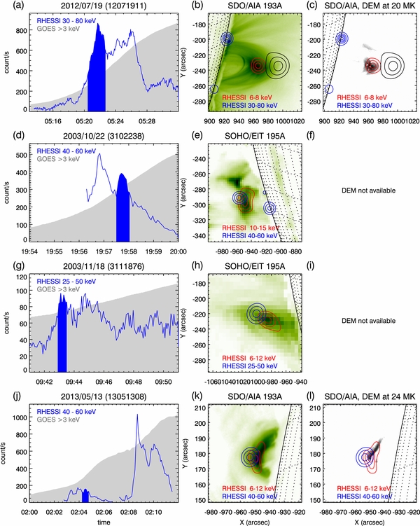
Figure 3. Overview of the four above-the-looptop sources. Left column: the time profiles of the non-thermal HXR count rate (blue curve) with the linear GOES profiles (shown schematically in gray in the background). Middle column: the EUV images (background) and the RHESSI CLEAN images (contours) generated for the time period indicated by the blue shaded region in the left column. For each image (colored separately by blue, red, or black), contours are shown for 50%, 70%, and 90% levels, except the footpoints of Case A, which additionally show 10% and 30% levels. The black contour in Panel (b) indicates the use of the two-step CLEAN method. See Table 2 for the parameters of the CLEAN images. Right column: the same RHESSI images (contours) with a DEM map in the background.
Download figure:
Standard image High-resolution image3.1.1. Imaging Analysis
To identify an above-the-looptop source, we generated X-ray CLEAN images (Hurford et al. 2002; Dennis & Pernak 2009). The back-projection images are used to determine an appropriate set of detectors (Table 2).
Table 2. Technical Parameters of the RHESSI Images in Figure 3
| Case | Energy, keV | Detectors | Beama |
|---|---|---|---|
| A | 6–8 | 5–8 | 2.2 |
| 30–80 (footpoint) | 3–5 | 1.0 | |
| 30–80 (coronal) | 5–9 | 1.0 | |
| B | 10–15 | 4–8 | 1.5 |
| 40–60 | 4–8 | 1.5 | |
| C | 6–12 | 5–8 | 1.8 |
| 25–50 | 6–8 | 2.2 | |
| D | 6–12 | 3–8 | 2.2 |
| 40–60 | 4–8 | 2.0 |
Note. aThe beam-width-factor parameter in RHESSI/CLEAN.
Download table as: ASCIITypeset image
In Figure 3(b), red and blue contours show the obtained CLEAN images in the 6–8 and 30–80 keV ranges, respectively. The background image is captured by the SDO/AIA 193 Å wavelength channel at 05:22:30 UT. The lower energy X-ray source is located at the looptop region. The higher energy X-rays were intense at the northern footpoint, but considerably weaker at the southern footpoint, as well as in the above-the-looptop region. Thus, we utilized the two-step CLEAN algorithm (Krucker et al. 2011) to obtain the faint coronal source in Figure 3(b).
It should be emphasized that although the looptop source (red contours) does not extend to the above-the-looptop region, that does not mean there is no 6–8 keV emission in the above-the-looptop source. We simply cannot form a clear image of 6–8 keV X-rays due to the limited dynamic range of RHESSI detectors. From the spectral fitting results presented later, we infer that the intensity of the 6–8 keV X-rays in the above-the-looptop source was at least an order of magnitude smaller than that of the looptop source.
Figure 3(c) shows the same CLEAN images, but the background now shows the differential emission measure (DEM) at ∼20 MK obtained by the SDO/AIA data. To calculate DEM, we used the regularized inversion code developed by Hannah & Kontar (2012). It is evident that that the feature in the DEM image outlines the looptop source. We note that our X-ray spectral analysis (described below) suggests a looptop source temperature ∼20 MK; the GOES temperature was ∼16 MK.
On the other hand, we did not find any spatial structure in the AIA images (both the data number (DN) images at various wavelengths and the DEM images at various temperatures) that shows the above-the-looptop source. Note that the DEM derived from AIA is not well constrained in a higher temperature range (≳107.3 K), whereas the RHESSI spectral analysis (presented in the next section) suggests a super-hot temperature ∼ 32 MK (=107.5) for the above-the-looptop source. Therefore, it is not surprising that AIA did not see a spatial structure that outlines the above-the-looptop hard X-ray source. The lack of spatial association between the relatively lower temperature emission (visible in both AIA and RHESSI 6–8 keV band) and the relatively higher temperature emission (visible in RHESSI >30 keV band) confirms that there are multiple plasma populations in the corona. Note that by using X-ray spectral analysis alone, Krucker & Lin (2008) has already suggested the existence of at least two distinct plasma populations in the corona.
3.1.2. Spectral Analysis of the HXR Data
To investigate non-thermal properties in the above-the-looptop source, we studied X-ray spectra by performing imaging spectroscopy as described by Krucker & Battaglia (2014). We generated CLEAN images at various energy ranges and then calculated photon flux in a fixed, polygonal region that contains both looptop and above-the-looptop sources. Because these coronal sources are well separated from the footpoint emissions, our conclusions presented in this paper are not sensitive to the choice of the polygonal region. On the other hand, the looptop and above-the-looptop sources are not well separated, especially in the intermediate range, 12–30 keV. Thus, the combined photon flux in the region must be studied as described below.
Figures 4(a)–(d) shows the combined photon flux in the histogram (identical in each row of panels). This observed energy spectrum is interpreted by assuming that there were two distinct plasma populations, one in the looptop region and another in the above-the-loop region (Krucker & Lin 2008). Here, a spectrum modeled for each population should be considered to be the mean spectrum of the emitting volume. Thus, the looptop source is represented by the thermal Maxwellian distribution (red curves), whereas the above-the-looptop source is represented by four different spectral models (blue curves): thermal, thermal+power law, kappa, and power law. In each panel, the two models (red and blue curves) are combined to produce the total spectrum (black curve) to be compared with the observation (histograms).
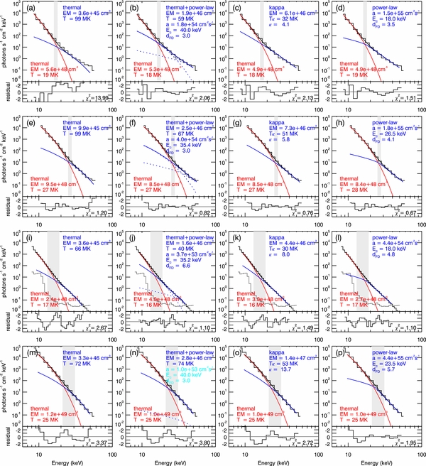
Figure 4. RHESSI spectral analysis of the combined coronal source (i.e., above-the-looptop and looptop sources). From top to bottom are Cases A (2012 July 19), B (2003 October 22), C (2003 November 18), and D (2013 May 13). A thermal distribution is used to represent the looptop source in all cases (red curves). Different models are used for the above-the-looptop source (blue curves) as shown in the four panels of each row; From left to right are the thermal, thermal+power-law, kappa, and power-law models. The dotted blue curves in the second column shows each component of the thermal+power-law model. The vertical gray bars indicate the energy range in which a separate imaging analysis showed comparable photon fluxes in the looptop and above-the-looptop sources. The initial values of the fittings are chosen so that the resultant curves (red and blue) intersect at an energy within the gray bar.
Download figure:
Standard image High-resolution imageThe spectral fitting was performed using OSPEX of Solar Soft Ware (SSW). For the kappa distribution, we used the program f_thin_kappa.pro (Kašparová & Karlický 2009). For the power-law distribution, we used the program f_thin2.pro (Holman et al. 2003). This program uses the flux distribution  (cm−2 s−1 keV−1), where a is the normalization coefficient, Ec is the lower-energy cutoff, and dFD is the power-law index.
We found that a range of values for parameters can fit the data equally well. For example, in Figure 4(c), the kappa temperature of the above-the-looptop source was 32 MK. However, by choosing different sets of initial values, we could fit the data equally well with smaller temperature and larger emission measure.
To constrain the models, we examined images at various energy ranges, and found that the photon fluxes of the looptop and above-the-looptop sources were comparable in the 16–18 keV range, as indicated by the vertical gray bar in Figures 4(a)–(d). Then, we tried different sets of initial values until the spectral fit agreed with the image of comparable fluxes (i.e., the red and blue curves intersect within the gray bar). As a result, we found that all spectral models except the thermal model could fit the data well. The fact that the "thermal" model alone could not fit the data indicates that non-thermal electrons did exist in the above-the-looptop source. However, we cannot constrain the three possible models from the RHESSI data alone.
3.1.3. Spectral Analysis of the EUV Data
To investigate whether we could further constrain the models, we examined EUV data obtained by the SDO/AIA instrument. The AIA data can be used to limit electron distribution functions in the lower energy range (<2 keV; e.g., Battaglia & Kontar 2013). The spectral models that fit the RHESSI data in the higher energy range, as discussed in Section 3.1.2 and Figures 4(a)–(d), can be extrapolated to the lower energy range to examine their consistency with the AIA data. The reconstruction of electron distributions is based on the DEM derived by the regularized inversion technique (Hannah & Kontar 2012). From a DEM profile, ξ(T)(= n2dV/dT), we can compute the mean density spectrum 〈nVF〉 in the emitting volume V
Note that we use density spectrum (electrons cm−3 keV−1), whereas Battaglia & Kontar (2013) use flux spectrum (electrons keV−1 s−1 cm−2).
A caveat here is that, as we discussed in Section 3.1.1, the lack of EUV spatial feature that outlines the above-the-looptop source indicates that there were two distinct plasma populations in the corona. The distribution reconstructed from the EUV data should represent the lower-temperature population and should be regarded as the upper limit of the distribution of the higher-temperature population. If otherwise, we should have seen an EUV spatial feature that outlines the above-the-looptop source.
Note also that we do not know the detailed shape of the above-the-looptop source due to the limited dynamic range of RHESSI images. In reality, the true above-the-looptop source may only contain one plasma population. However, if we cutout the above-the-looptop region based on an ad hoc definition derived by a RHESSI image contour, then such a region may encompass regions of another plasma population. Therefore, any distribution reconstructed for our purpose depends on how we define the above-the-looptop region or how we choose the filling factor f.
Let us first consider the 50% contour (i.e., the outermost black contour in Figures 3(b) and (c)) and define this as the case of filling factor f = 1. This is the simplest case and gives us the most optimistic upper limit, as this upper limit can be lower depending on the actual value of f.
Figure 5(a) shows the DEM profile obtained by using the AIA pixels within the 50% RHESSI contours. (See Battaglia & Kontar 2013 and Krucker & Battaglia 2014 for more details of the DEM profile.) There is a lower temperature peak (1.4–2.0 MK) and a higher temperature peak (10–14 MK). It has been interpreted that the lower temperature component corresponds to the foreground and background plasmas, whereas the higher temperature component is flare-related (Krucker & Battaglia 2014). Therefore, we only use the higher temperature peak (i.e., the TM > 106.5 K range) to reconstruct the distribution.
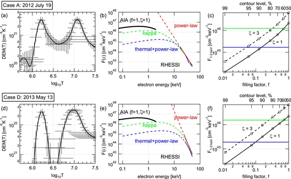
Figure 5. Reconstruction of electron distributions for Cases A (upper panels) and B (lower panels). Left (a and d): DEM profiles obtained by the regularized inversion code. Middle (b and e): Electron distributions reconstructed from the DEM (black curve) and RHESSI spectral fit (colored curves). The dashed curves show extrapolations of the fitted curves. Right (c and f): The differential density level as a function of filling factor f (bottom axis) or RHESSI contour level L (top axis).
Download figure:
Standard image High-resolution imageFigure 5(b) black curve shows the reconstructed distribution for the case of f = 1. This curve is almost identical to the curve of isothermal Maxwellian with TM = 107.1 K (not shown). Also shown (by colored solid curves) are the differential density spectra reconstructed by using parameter values obtained by the spectral analysis (described in the previous subsection). If we extend these distributions to the lower energy range (colored dashed curves), we can see that the thermal+power law and kappa are consistent with the upper limit.
Perhaps, this optimistic upper limit (as shown in Figure 5(b)) is still underestimated. As has been noted by Battaglia & Kontar (2013) and Krucker & Battaglia (2014), the regularized inversion code has a tendency to underestimate DEM profiles by roughly a factor of ζ = 2–3. The uncertainties in the AIA temperature response do not allow us to implement an empirical correction. In Figure 5(b), we simply plotted the case of ζ = 1 (i.e., no correction). Whatever value ζ takes, we can safely conclude that both the thermal+power-law and kappa models are plausible if f = 1.
It should also be noted that we may need to consider different temperature responses for non-thermal plasmas. We verified that temperature responses developed by Dudík et al. (2009) modify the reconstructed distribution only slightly. This is probably because DEM ξ(E) affects the distribution through an integral (see Equation (5)). The uncertainties expressed as f and ζ are of greater concern.
Let us now consider cases with f < 1. This consideration would not allow us to further constrain the spectral models, but it can give us an order estimate of the filling factor f and thus a better estimate of the number density in a later section of this paper. Recall that the filling factor f represents the fact that the X-ray imaging has a limited spatial resolution. The actual source size may be smaller and may contain substructures that cannot be identified by the current observation. Here, we make an assumption that the source does not have substructures and can be modeled by different levels of RHESSI contour. Then, we reconstructed the distribution using AIA pixels within L% RHESSI contour, where L = 50%, 60%, 70%, 80%, 90%, 95%, and 99%. For each L, we computed the area A(L) within the contour and derived the filling factor as f = A(L)/A(50).
Figure 5(c) shows the resultant differential density averaged in the 1–2 keV range as a function of f (bottom axis) and L (top axis). The solid and dashed lines show results for ζ = 1 and 3, respectively. In the case of ζ = 3, for example, the differential density becomes as small as the level predicted by the kappa model (the horizontal green line) when f reaches ∼0.3. The range f < 0.3 is unlikely, under the assumption of the kappa model because the differential density of the kappa distribution becomes larger than that derived from the AIA images. In such case, we should have seen an EUV spatial feature that outlines the above-the-looptop source. We can still have f as small as 0.06 under the assumption of the thermal+power-law model because the differential density predicted by the thermal+power-law model (the horizontal blue line) is smaller than that of the kappa model. Note, however, this smaller differential density comes from the smaller emission measure obtained as an artifact of the lower-energy cutoff Ec (see Section 2).
3.2. Case B of the 2003 October 22 Flare
Case B, 2003 October 22 flare, is another example of a clearly non-thermal, above-the-looptop source (Ishikawa et al. 2011). Figure 3(d) shows the time profile of the hard X-rays measured by RHESSI. Following Ishikawa et al. (2011), we analyze data from the period 19:57:30 to 19:58:02 UT, which showed an intense emission from the above-the-looptop source.
Figure 3(e) shows the RHESSI contours taken during this X-ray flux peak time (19:57:30–19:58:02 UT) with the same format as Figure 3(b). The two-step CLEAN is not used and the background image was captured by the SOHO/EIT 195 Å wavelength channel at 19:57:30 UT. The above-the-looptop source (off-disk blue contours) is clearly visible. The coronal sources (both the above-the-looptop and looptop sources) are well separated from the footpoints. Then, we made images at 16 different energy ranges and used the combined flux of the above-the-loop and looptop sources to obtain an energy spectrum.
Figures 4(e)–(h) show the result of this imaging spectroscopy with the same format as Figures 4(a)–(d). As in Case A, we constrained each spectral model by finding an energy range that shows comparable fluxes in above-the-loop and looptop sources (shaded gray bars). Again, all non-thermal models fit the data well. The thermal model alone could not fit the data, especially in the higher energy range (>50 keV) and resulted in a chi-square value higher than that of other models. Therefore, we consider that this flare produced an enhanced non-thermal tail in the above-the-looptop source. The SDO/AIA data are not available for this flare, so we cannot constrain the models any further.
3.3. Case C of the 2003 November 18 Flare
Case C is obtained during the GOES M4.5 flare on 2003 November 18. This flare was unique in that it clearly showed an apparent current sheet between the flaring loop and the upward moving ejecta (Lin et al. 2005). This flare was also one of the events analyzed statistically by Krucker & Lin (2008).
Figure 3(g) shows the time profile of the count rates of the 25–50 keV X-rays. There are several major enhancements and we take the time period of most intense count rates, 09:42:54–09:43:32 UT. Figure 3(h) shows the RHESSI images with the same format as Figure 3(b). The footpoints were not detected, indicating that they were behind the solar limb (or occulted).
As for spectral properties of this above-the-looptop source, we used a spatially integrated spectrum rather than imaging spectroscopy because the footpoint emission was not detected. Figures 4(i)–(l) show the spectral analysis with the same format as other cases, but with the background spectrum shown in gray.
Unlike Cases A and B, the thermal model (Figure 4(i), blue curve) can roughly fit the data, although the χ2 was relatively larger than the result of other models. However, the addition of a power-law tail (i.e., thermal+power-law model) improved the fit, suggesting the presence of a non-thermal tail (Figure 4(j), blue curve). The kappa model could also fit the data equally well (Figure 4(k), blue curve) although the resultant kappa value was somewhat large ∼8. These results suggest a slightly enhanced non-thermal tail. The power-law model could also fit the data well, but the power-law index dFD(∼ 4.8) was somewhat larger than that of Case A (dFD ∼ 3.5) and B (dFD ∼ 4.1), again indicating that the non-thermal component was less significant compared to that of Cases A and B.
The SDO/AIA data is not available for this flare, so we cannot constrain the models any further.
3.4. Case D of the 2013 May 13 Flare
On 2013 May 13, the same active region produced two X-class flares at ∼02:10 UT (X1.7) and ∼16:00 UT (X2.8; Martínez Oliveros et al. 2014; Saint-Hilaire et al. 2014). In this paper, we focus on a time period from the first flare, which will hereafter be described as Case D.
Figures 3(j)–(l) shows the overview. The X-ray count rate showed major enhancements at 02:04 UT and 02:09 UT (Figure 3(j)). Because the second enhancement was dominated by footpoint emissions (not shown), we analyzed the data from the earlier enhancement during which we could safely isolate the above-the-looptop source (Figures 3(k) and (l)). There is a faint source near the northern footpoint at (X,Y)(−940,190) (visible in the 10%–30% contours, not shown). To avoid this faint source, we again use imaging spectroscopy to focus on the looptop and above-the-looptop sources.
Figures 4(m)–(p) shows the result of imaging spectroscopy. As in Case C, the thermal model (Figure 4(m), blue curve) can fit the data roughly well, suggesting a less enhanced non-thermal tail. Unlike Case C, the thermal+power law did not improve the fit. The kappa model could also fit the data well (Figure 4(o)), but the kappa value was very large κ ∼ 15, indicating that the spectrum is close to Maxwellian. The power-law model with no thermal core could also fit the data well (Figure 4(p)), but the power-law index dFD(∼ 5.7) was significantly larger than that of Case A (dFD ∼ 3.5) and B (dFD ∼ 4.1), indicating that the non-thermal component was less significant compared to that of Cases A and B.
Figure 5(d) shows the AIA/DEM profile obtained within the area defined by the 50% RHESSI contour in the 40–60 keV range. The obtained DEM profile exhibits a double peak structure similar to that of Case A. Here, a positivity constraint is used. Figure 5(e) shows the derived optimistic upper limit (black curve), as well as the various spectral models used to fit the RHESSI data (colored curves). Again, the thermal+power-law and kappa models do not contradict the derived upper limit when f = 1. The possible range of f is investigated in Figure 5(f). For the kappa model, f should be ≳0.3 (when ζ = 3). For the thermal+power-law model, f should be ≳0.03 (when ζ = 3).
4. DISCUSSION
In the previous section, we analyzed four cases of the above-the-looptop source that are typically visible in the ≳15 keV range. We found two cases with significantly enhanced high-energy tails and two cases with less enhanced tails. The thermal distribution did not fit the data well in the enhanced cases, indicating the presence of non-thermal component. The power law alone could also fit the data, but it requires the lower-energy cutoff Ec at ∼20 keV. To fill the gap below Ec, a hot thermal core can be considered. We found that the kappa model can fit the RHESSI data. In two cases with unsaturated EUV data from SDO/AIA, the analysis of DEM did not rule out the kappa distribution model. The thermal+power-law model could also fit the RHESSI data, but the resultant temperatures (TM = 40–74 MK) were systematically higher than those obtained by the kappa model (Tκ = 30–53 MK). Similarly, the emission measures obtained by the thermal+power-law model (EM ∼ (1.6–2.8) × 1046cm−3) were systematically lower than those of the kappa model (EM ∼ (4.4–14) × 1046cm−3). We attribute these systematic differences to the artifact of having the lower-energy cutoff Ec in the model (see Section 2). Therefore, when compared to conventional spectral models that contain the artifact, the kappa distribution model seems to be a natural and better choice for interpreting the observed hard X-rays from the above-the-looptop source. For simplicity, we simply use the results of the kappa distribution fit in the discussions below.
4.1. Non-thermal Fraction of Electron Energies
Table 1 summarizes the obtained κ as well as the computed non-thermal fractions RN and Rε of electron number density and energy density, respectively. The largest values of RN and Rε are 19% and 49%, respectively. Note that for another case study of the 2007 December 31 flare, RN ∼ 20% and Rε ∼ 51%. Therefore, we speculate that there might be an upper limit for RN at 20% and Rε at 50%. The limit Rε = 50% means equipartition of electron energies between thermal and non-thermal components. We need a larger number of events to establish this idea of upper limit at equipartition of energies. We think that such an upper limit would exist because the highest energy particles can constantly escape from the acceleration region. More theoretical studies are needed to understand the possible upper limit of the energy partition.
The total electron energy density εe can be estimated as εe ≡ (3/2)NTκ where N is the total electron density and Tκ is the kappa temperature. Note again that, by definition Tκ contains contributions from non-thermal electrons (Oka et al. 2013, and references therein). The energy density of non-thermal electrons can then be estimated as Rεεe. The resultant values are 3–15, 5–60, 2–15, and 10–60 erg cm−3 for Cases A, B, C, and D, respectively.
4.2. Electron Energization Mechanism
Many ideas have been proposed to explain energetic electrons associated with the above-the-looptop source (see a review by, for example, Krucker et al. 2008). In a standard picture of solar flares, magnetic reconnection plays an important role for converting the coronal magnetic energies into plasma energies and it has been known to provide an efficient mechanism for electron energization (e.g., Hoshino et al. 2001; Pritchett 2006). Furthermore, because a fast-mode termination shock may be generated as a consequence of the downward reconnection jet colliding with the flaring loop, the energetic electron flux may be enhanced at the shock (e.g., Masuda et al. 1994; Tsuneta & Naito 1998; Aurass et al. 2002), although more recent observations indicate a deceleration of supra-arcade downflows (e.g., Sheeley et al. 2004). Additional energization may also occur through the Fermi and betatron type mechanisms in the collapsing reconnected fields (e.g., Somov & Kosugi 1997) or through turbulence (e.g., Miller et al. 1997). It is beyond the scope of this paper to consider all existing theories and compare them with our observations.
Here, we focus on magnetic reconnection as a starting point. If magnetic reconnection proved to be insufficient to explain the electron distributions deduced from our analysis, then we would need additional mechanisms such as those attained by shocks, collapsing fields, and turbulence. However, we show below that a two-dimensional (2D) particle-in-cell (PIC) simulation of magnetic reconnection can already produce energy spectra very similar to those obtained in our analysis.
In general, a 2D PIC code can simulate multiple X-lines that evolve as a natural consequence of the tearing-mode instability of a current sheet. The non-linear evolution of the current sheet leads to multi-island coalescence, and the contracting motion of a freshly merged magnetic island can energize electrons by the Fermi kicks at each end of the island (Drake et al. 2006; Bian & Kontar 2013). Electrons can also be energized at the merging point where a secondary reconnection takes place (Oka et al. 2010b). The secondary reconnection is, in a sense, internally driven by the two colliding islands converging at the speed of a reconnection jet. As a result, electrons are significantly heated and a non-thermal tail also appears.
In this section, we compare our observations with the multi-island coalescence model (Oka et al. 2010a, 2010b). The simulation setup can be summarized as follows. The simulation is run by a 2.5D, fully relativistic PIC code that does not model Coulomb collisions. The initial condition consists of two Harris current sheets to allow periodic boundaries in both directions. The ion inertial length di is resolved by 25 cells so that D = 0.5di and Lx = Ly = 102.4di, where D is the half-thickness of the current sheet and Lx, Ly are the domain size in  and
and  direction, respectively. The ion to electron mass ratio mi/me = 25 and the light speed c is 15 VA, where VA is the Alfvén speed defined as B
 . We used an average of 64 particles in each cell. The unit density is represented by 297 particles per cell. No magnetic field perturbation is imposed at the beginning so the system evolves from the tearing mode instability due to particle noise.
Figure 6(a) shows the electron energy spectrum obtained by the simulation.6 In the code the electron energies were normalized by the rest-mass energy (bottom axis), but an unrealistic value was used for their initial temperature due to a limited computational resource. Thus, we re-normalized the electron energies by the average energy εth of the inflowing electrons at time T = 0 (top axis).7.
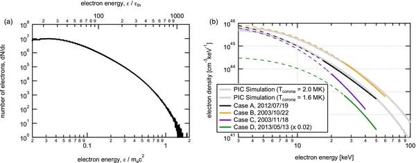
Figure 6. Comparison between PIC simulation and RHESSI spectra (kappa fit). (a) PIC simulation energy spectrum with electron energies normalized by the rest mass energy (bottom axis) and initial thermal energy (top axis). (b) PIC simulation energy spectra with assumed initial thermal energies Tcorona (gray curves) are compared to the kappa fit results of the RHESSI spectra (colored curves).
Download figure:
Standard image High-resolution imageFigure 6(b) shows the comparisons between the simulated spectrum and the spectra reconstructed from the result of the kappa model fit to the above-the-looptop source component (i.e., blue curves of Figures 4(c), (g), (k), and (o)). For the simulated spectrum, a coronal temperature Tcorona can be used to convert ε/εth to keV. For Case A, we assumed Tcorona = 1.6 MK taken from the lower temperature peak of the DEM, which is likely to be representing foreground/background (Figure 5(a)). For Case B, the AIA/DEM is not available, so we assumed the typical coronal temperature Tcorona = 2.0 MK. We also shifted the simulated spectra arbitrarily in the vertical axis direction because one particle in a PIC simulation represents an arbitrary number of real particles. As a result, the spectra from the simulation (dark and light gray curves) agreed roughly well with the spectra from Cases A and B (black and orange curves).
The simulation is, of course, not realistic in many ways. For example, the simulation was limited in 2D. The guide field (i.e., the out-of-plane component of the initial magnetic field) was zero. Also, the initial plasma β (= 0.2) was somewhat large. A possible particle escape via turbulence has been neglected. These unrealistic settings may have accidentally led to the rough agreement with the observation. Furthermore, the above-the-looptop region is not necessarily the magnetic reconnection region, and there could be additional energization mechanisms as mentioned above (i.e., energization by the fast termination shock, collapsing fields, turbulence, etc.). Modification of the energy spectrum by scattering and escape should also be considered. Therefore, in future studies, we need a systematic and parametric survey of spectra using simulations with possible and realistic conditions for the proposed energization mechanisms.
Nevertheless, the rough agreement between the observation and a simple reconnection simulation suggests that magnetic reconnection alone can already attain non-thermal energies (up to >50 keV) observed in the above-the-looptop region. In this regard, it is interesting that a study of microwave emission reported hardest spectra at and near the X-point seen in the soft X-ray (Narukage et al. 2014). Furthermore, we emphasize that magnetic reconnection may be equally important in Cases C and D in which electrons were heated to a very high temperature (30 and 53 MK, respectively, based on the kappa model fit), although the non-thermal tail was not clearly identifiable. The simulated spectra in Figure 6 indicates that magnetic reconnection can produce not only non-thermal component but also a high temperature thermal component. Therefore, although a non-thermal tail is not always clear in the observations of above-the-looptop sources, solar flares in general may produce a superhot thermal plasma by magnetic reconnection. This is consistent with the idea of a super-hot coronal source (Longcope et al. 2010; Caspi & Lin 2010).
4.3. Collisionality
The spectral analysis in Section 3 indicates that the non-thermal tail was clearly enhanced in Cases A and B but not in Cases C and D, although the temperature was equally high (super-hot) in all four events. What made the difference? Here, we consider the possibility that larger densities in Cases C and D made them collisional even for the high energy (>10 keV) electrons, and such non-negligible collisionality in the above-the-looptop source has prevented the enhancement of the non-thermal tail. In fact, Galloway et al. (2010) showed that the non-thermal, high-energy tail of a kappa-like distribution can be thermalized into Maxwellian over the timescale of 100–1000 τcoll, where τcoll is the electron-electron collision time of the core particles.
Figure 7 summarizes our estimation of electron number densities in the above-the-looptop sources (blue parallelograms). We evaluate an electron number density N as
where EM is the emission measure and V is the source volume. We consider a columned volume V = fAd, where f is the filling factor, A is the source area measured from the 50% level contour of the RHESSI images, and d is the source depth.
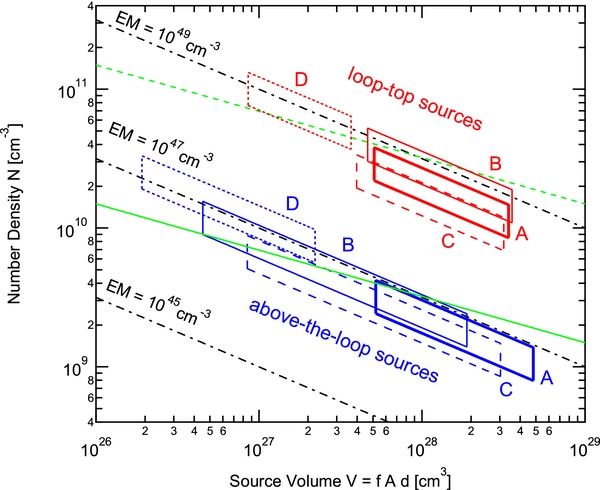
Figure 7. Estimated ranges of source volume V and electron number density  . The green dashed line represents the critical density Ncrit above which a non-scattering source becomes collisional for electron energies above 30 keV. The solid green curve shows a case with turbulent scattering (i.e.,
  ).
).
Download figure:
Standard image High-resolution imageFor the EM, we used the values obtained by the kappa model fits (see values indicated at the upper-right corners of the panels of Figure 4 third column). We assumed a relatively large (50%) uncertainty for the EM in all cases and it is represented as the height of the parallelograms in Figure 4.
For the filling factor f, we used f = 1 for its upper limit. For the lower limit, we used f = 0.3 and 0.2 for Cases A and D, respectively, as constrained from AIA/DEM discussed in Section 3. For the other events, we used a similar value f = 0.1. In these cases, f can be smaller but it should not be too small, say f < 0.01, because otherwise the energy density of the source would far exceed that of the coronal magnetic field.
For the source depth d, we used an approximate size of the above-the-looptop source for the lower limit dmin. The upper limit dmax can be the length of the flare ribbon or arcade as seen from STEREO/EUV (Krucker & Battaglia 2014). For Cases A and D, we estimated it to be about 100'' and 50'', respectively. There is no stereoscopic observation for Cases B and C, so we simply used the larger size of the other two events (i.e., 100'').
Figure 7 shows that within the assumed uncertainties, the density of Case D with steep spectrum, (0.6–3.3)× 1010cm−3, is an order of magnitude larger than that of Case A with flat spectrum, (1–4) × 109 cm−3. The densities of Cases B and C are in between the two ranges, but have nearly two orders of magnitude uncertainties. Thus, we propose that Cases C and D were too collisional to sustain non-thermal tail.
Let us then consider a critical density Ncrit above which a source becomes collisional for a particle with energy E. For simplicity, we further approximate the columned volume as a sphere so that the size of the source can be expressed as L = 2(3V/4π)1/3. For the source to be collisional, L has to be larger than the mean free path λmfp, coll = vτcoll, where v is the particle speed and τcoll = 3 × 10⁻²⁰v3/N seconds (Benz 1993). Then, the critical density can be estimated as
This critical density N(V) for a fixed energy E = 30 keV is shown in Figure 7 as a green dashed line. We chose E = 30 keV because the non-thermal tail in Cases A and B are seen roughly above 30 keV. Then, we can see that the estimated density range (shown in the blue parallelograms) are below the green dashed line, meaning Cases A, B, C, and D were all collisionless. This is inconsistent with our scenario that Cases C and D were too collisional for the non-thermal tail to develop.
However, we can further consider an effect of scattering due to electromagnetic waves, turbulence, or sub-structures within the source region. Such scattering leads to trapping of particles within the source and allows them to have a greater chance of colliding with each other. The mean free path and hence the critical density can become smaller, so that  where α < 1.
The solid green line in Figure 7 shows the case of α = 0.1. Because the solid green line is now roughly separating the density ranges of the two different types of sources, our proposed scenario (i.e., the collisionality led to suppression of non-thermal tail) still holds.
It is worth noting again that for Case D of the 2013 May 13 flare we selected a time period when the flaring footpoints were not visible. The relatively high collisionality may have prevented the high-energy electrons from propagating to the footpoints. Also, this case may be closely related to the so-called coronal thick target events (e.g., Veronig & Brown 2004).
5. SUMMARY AND CONCLUSION
We analyzed four cases of the above-the-looptop source and found two cases of significantly enhanced non-thermal tails (Cases A and B) and two cases of less enhanced non-thermal tails (Cases C and D). We argued that the electron spectrum in the above-the-looptop source exhibits a saturated non-thermal tail connected smoothly to the hot thermal core without any spectral brake. This distribution can reasonably be modeled by the kappa distribution model. The thermal+power-law model systematically overestimates and underestimates the temperature and density, respectively, due to the lower-energy cutoff Ec.
Based on the kappa model, we found that the 2012 July 19 flare (Case A) showed the largest non-thermal fraction of electron energy, ∼49%. This is similar to the value ∼51% obtained for the 2007 December 31 flare (Oka et al. 2013). Therefore, we speculate that the non-thermal fraction of electron energy has an upper limit at ∼50%, meaning equipartition of energies, although we need a larger number of non-thermal events to establish this idea. We speculate that such an upper limit can exist because the highest energy particles can constantly escape from the acceleration region. More theoretical studies are needed to understand the possible upper limit of the energy partition.
For the cases of a significantly enhanced non-thermal tail, the observed energy spectrum roughly agreed with the properly normalized energy spectrum obtained by a 2D PIC simulation of magnetic reconnection (i.e., a multi-island coalescence model), suggesting that magnetic reconnection alone can achieve the non-thermal energies (>80 keV) despite the simplifications and assumptions used in the simulation.
For the cases of less enhanced non-thermal tails, the temperatures were still high, 30 MK for the 2003 November 18 flare (Case C) and 53 MK for the 2013 May 13 flare (Case D), suggesting that a large fraction of magnetic field energies were released during these flares. Also, the case of least enhanced non-thermal tail (Case D) was estimated to have a number density that was an order of magnitude larger than that of the most enhanced non-thermal tail (Case A). Thus, we propose a scenario that electron energization is achieved primarily by collisionless magnetic reconnection, but the non-thermal tail can be suppressed or thermalized by Coulomb collisions. This scenario requires a turbulent scattering that is strong enough to reduce the mean free path by an order of magnitude in case of, for example, 30 keV electrons.
We thank Jaroslav Dudík for drawing our attention to the different representations of the thermal core component and also for kindly providing us temperature response functions for the kappa distribution. We acknowledge the use of the DEM code developed by Iain Hannah. We thank Iain Hannah, Marina Battaglia, and Lindsay Glesener for their helpful comments on the use of the code. We thank all members of the RHESSI, SDO, and SOHO projects for providing the data. This work was supported by NASA contract NAS 5-98033 for RHESSI. M.O. was supported by NASA grant NNX08AO83G at UC Berkeley.
Facilities: RHESSI - Ramaty High Energy Solar Spectroscopic Imager satellite, SDO (AIA) - Solar Dynamics Observatory, SOHO (EIT) - Solar Heliospheric Observatory satellite.
APPENDIX: DEFINITIONS OF THERMAL AND NON-THERMAL COMPONENTS
There are at least two reasonable ways to define the thermal and non-thermal components in the kappa distribution. In this section, we describe the two definitions and explain why we prefer one definition to another.
One definition is to use an adjusted Maxwellian distribution as the thermal core component, as adopted in Oka et al. (2013) as well as throughout this paper. The temperature of the Maxwellian distribution TM is adjusted so that its most probable energy Emp(= kTM) matches that of the kappa distribution,
Similarly, the number density NM is adjusted so that the differential flux at Emp matches that of the kappa distribution. Namely,
Figure 8(a) illustrates the non-thermal component in this definition (shaded in blue). Note that Emp separates the non-thermal component into the lower-energy and higher-energy populations. The separation can be more clearly illustrated by taking the difference, as shown in Figure 8(c). However, the total number of the lower-energy population is orders of magnitude smaller than that of the higher-energy population.

Figure 8. Two possible definitions of the non-thermal component in the kappa distribution. The cases with an adjusted core (blue) and asymptotic core (red) are shown in panels (a) and (c), respectively. The difference between the kappa distribution and the core (equivalently the differential density of the non-thermal components) are shown in panels (b) and (d). Panel (e) shows that the non-thermal fractions of number density (solid curves) and energy densities (dashed curves) are higher in the case of the asymptotic core (red curves) when compared to the case of adjusted core (blue curves). Tκ = 100 MK and κ = 2.4 are used in panels (a–d). The non-thermal fractions (shown in panel (e)) are functions only of κ.
Download figure:
Standard image High-resolution imageAnother definition is to use the low-energy asymptotic limit of the kappa distribution (see Equation (12) of Livadiotis & McComas 2009),
Accordingly, for the core component to approach the kappa distribution in the low-energy limit, the density should be
Figure 8(b) illustrates the non-thermal component in this definition (shaded in red). If we take the difference between the kappa distribution and the asymptotic core distribution (Figure 8(d)), a peak appears at an energy closer to Emp. The total number of non-thermal particles is larger than that of the case with adjusted core. This can be more clearly illustrated by comparing the non-thermal fractions as a function of κ.
Figure 8(e) illustrates the non-thermal fractions of number density (RN, solid curves) and energy density (Rε, dashed curves) for the cases of the adjusted core (blue curves) and asymptotic core (red curves). It is evident that the definition with asymptotic core gives systematically larger non-thermal fractions. At κ ∼ 4, Rε ∼ 50% in the definition with the adjusted core, whereas Rε ∼ 68% in the definition with the asymptotic core.
While the definition with the asymptotic core component is mathematically simple, we prefer the definition with the adjusted core. This is because, in the definition with the asymptotic core, a large part of the non-thermal population resides in the energy range close to Emp where the spectral shape does not exhibit a power law. This is counterintuitive. In the example case of Figures 8(b) and (d), 40% of the non-thermal particles has energies less than 10 keV.
The choice of definition is rather subjective and is made for convenience. In this paper, we suggested that the minimum value of κ in the above-the-looptop source may be ∼4 and we interpreted the value as the equipartition of energies between thermal and non-thermal components. It is important to examine a larger number of events to establish the idea of minimum κ at ∼4 and to continue our effort to understand the precise and theoretical meaning of the κ values.
Footnotes
- 4
This kappa distribution is equivalent to the modified kappa distribution formulated by Leubner (2004). The transformation can be expressed as κ* = κ + 1 and
 , where κ* and θ* are the spectral index and the most probable speed of the modified kappa distribution, respectively (Livadiotis & McComas 2009).
 - 5
Note that even if we considered a power-law population injected from an external source, it still needs to co-exist and/or interact with the pre-existing population within the above-the-looptop source. In general, this external-origin scenario considers the injected population to be more tenuous than the pre-existing, mostly thermal population (e.g., Holman et al. 2011) and should be examined by the thermal+power-law model (i.e., Figures 1(b) and (c)).
- 6
- 7
The initial setup of the simulation contained two plasma populations (i.e., background and current sheet plasmas with temperatures Tbk and Tcs (= 5Tbk), respectively). Because particles in the initial current sheet were eventually pushed away by the reconnecting plasma, it is the background population that flows into the reconnection region and experiences energization. Therefore, in Figure 6(a), we used Tbk for the normalization. Oka et al. (2010b) inappropriately used Tcs for the normalization in Figure 12 of their paper.