


ABSTRACT
Continuing our series of observations of coronal motion and dynamics over the solar-activity cycle, we observed from sites in Queensland, Australia, during the 2012 November 13 (UT)/14 (local time) total solar eclipse. The corona took the low-ellipticity shape typical of solar maximum (flattening index ε = 0.01), a change from the composite coronal images we observed and analyzed in this journal and elsewhere for the 2006 and 2008–2010 eclipses. After crossing the northeast Australian coast, the path of totality was over the ocean, so further totality was seen only by shipborne observers. Our results include velocities of a coronal mass ejection (CME; during the 36 minutes of passage from the Queensland coast to a ship north of New Zealand, we measured 413 km s−1) and we analyze its dynamics. We discuss the shapes and positions of several types of coronal features seen on our higher-resolution composite Queensland coronal images, including many helmet streamers, very faint bright and dark loops at the bases of helmet streamers, voids, and radially oriented thin streamers. We compare our eclipse observations with models of the magnetic field, confirming the validity of the predictions, and relate the eclipse phenomenology seen with the near-simultaneous images from NASA's Solar Dynamics Observatory (SDO/AIA), NASA's Extreme Ultraviolet Imager on Solar Terrestrial Relations Observatory, ESA/Royal Observatory of Belgium's Sun Watcher with Active Pixels and Image Processing (SWAP) on PROBA2, and Naval Research Laboratory's Large Angle and Spectrometric Coronagraph Experiment on ESA's Solar and Heliospheric Observatory. For example, the southeastern CME is related to the solar flare whose origin we trace with a SWAP series of images.
Export citation and abstract BibTeX RIS
1. INTRODUCTION
The properties of the white-light corona (WLC) are governed by the large-scale magnetic field of the Sun, for which we have only indirect measurements, though future missions, including Solar Probe+ and Solar Orbiter, are planned to sample closer to the Sun than previously possible. The shape of the WLC is sensitive to the phase of the solar activity cycle (Golub & Pasachoff 2010, 2015; Pasachoff 2009a, 2009b).
We present here the results of the observations of the WLC during the 2012 total solar eclipse. The eclipse appears in the catalogues as November 13 (UT), which translated to the early morning of November 14 locally for both observing sites reported here. Our main teams were stationed at the position of longest totality available from the ground (avoiding observations from the unstable platform of a ship): the northeast Queensland coast of Australia near Cairns and Port Douglas. We compare our results with images obtained from a ship (Pacific Venus in Figure 1) in the Pacific Ocean north of New Zealand to look for temporal changes, and with the corresponding spaceborne observations. We reported preliminary results to the Solar Physics Division of the American Astronomical Society (Pasachoff et al. 2012).
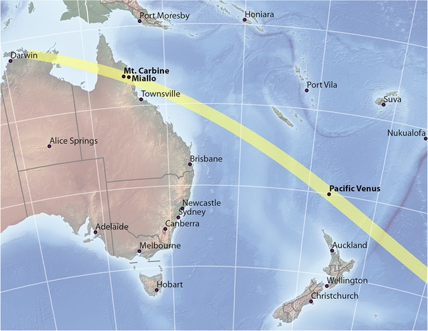
Figure 1. Map showing the path of totality of the 2012 November 13/14 eclipse (November 14, local date and time). Ground-based observing sites such as Mt. Carbine and Miallo are located near the northeast coast in Queensland, Australia. (Courtesy: Michael Zeiler, eclipse-maps.com).
Download figure:
Standard image High-resolution imageOur comparisons are similar in method to those we reported from pairs of observing sites at the 2006 eclipse (Pasachoff et al. 2007, 2008) from Greece; at the 2008 eclipse (Pasachoff et al. 2009) from Siberia; at the 2009 eclipse (Pasachoff et al. 2011b) from China; and at the 2010 eclipse (Pasachoff et al. 2011a) from Easter Island. But only with this 2012 total solar eclipse did the Sun approach the maximum phase of the solar-activity cycle, so the corona was in a different configuration. As with the 2010 eclipse, our comparison data benefitted from an erupting coronal mass ejection (CME). We again take advantage of observations made by the current generation of solar spacecraft, including instruments on NASA's Solar Dynamics Observatory (SDO), JAXA's Hinode, and ESA's Project for Onboard Autonomy 2 (PROBA2), as well as full-Sun coverage, including the whole far side, from NASA's Solar Terrestrial Relations Observatory (STEREO), which also supplied outer coronal views from its pair of perspectives.
2. BASIC INFORMATION ON THE 2012 NOVEMBER 13/14 ECLIPSE OBSERVATIONS
The path of totality started in the Australian outback and reached the northeast Queensland coast with the Sun at only 13° altitude. The rest of the path was entirely over the Pacific Ocean (Figure 1; Jubier 2012a, 2012b; Espenak & Anderson 2012; Zeiler 2012; Golub & Pasachoff 2014). No airborne expeditions intercepted the path, except for our helicopter. Only passengers on ships saw totality after it left the Queensland coast and adjacent islands.
We chose our original observing site while relying on the cloud statistics from J. Anderson (2012, private communication) and F. Espenak & J. Anderson (2012, private communication). We noted also that the low altitude of totality, 13°, could lead to potential obscuration by clouds that do not show well on the satellite views that went into the statistical calculations.
2.1. Mt. Carbine
Our observation site at Mt. Carbine was at 16°16'22'' S latitude and 144°42'53'' E longitude, on the Tablelands, inland from the Queensland coast, with 2 m 2 s of totality, centered at 20:38:49 UTC. Part of our observing team, headed by B.A.B., reconnoitered there the day before the eclipse and stayed the night before the early morning eclipse, because of the high probability expected for the eclipse-time cloudiness of our long-term Miallo site. The image shown in Figure 2 was made from 58 individual frames from a RED Epic (www.red.com/products/epic) IMAX-quality, high-resolution camera operated by R.D. and Nicholas Weber. (We discuss the image processing by P.G., which included the use of darks and flats, in Section 3 of this paper.) We have additional Nikon D90+Nikkor 500 mm lens frames taken by B.A.B.

Figure 2. Combination of 58 white-light corona images taken by R.D. and Nicholas Weber at Mt. Carbine, Queensland, Australia, and computer-processed by P.G. Solar north, east limb, and position angles (P.A.s) around the solar limb are labeled in white. A tennis-racquet-shaped structure is labeled TR; it is discussed in Section 5.
Download figure:
Standard image High-resolution imageThere was also a slitless spectrograph at this last-minute site. Its data were recorded with a second RED Epic camera, to continue the studies of coronal temperature from the [Fe x]/[Fe xiv] ratio, as previously reported by our group (Voulgaris et al. 2010, 2012). The RED Epic camera has a high dynamic range of 13.5 stops, up to 120 fps at 5k resolution with an effective 13.8 megapixel 14 bit CMOS sensor. The minimally compressed REDCODE RAW digital format preserves the original color space. We acquired the WLC and spectral images at 24 fps from C1 (first contact) to C4 (fourth contact). Relevant frames were adjusted for exposure and ISO values, then exported as TIFF files for image processing.
2.2. Miallo Observations
On a reconnoitering trip a year in advance, we had found a house about 10 km inland from Newell in the town of Miallo. It was at a few hundred meters of altitude, to provide a sweeping view of the shadow's departure, as well as the low-altitude totality above the ocean.
Early morning observations at eclipse time over the week preceding totality did not give hope for clear eclipse weather, so a group took much of our equipment inland, as discussed in Section 2.1. Some observers remained at Miallo in case suitable holes in the clouds allowed the use of our best-calibrated equipment on the best-aligned mounts; that work was supervised by M.L.
When the weather looked definitively cloudy about half an hour before totality, J.M.P. and Robert Lucas went aloft in a helicopter that we had arranged previously to stand by. (We were joined by a BBC camera operator who was filming a documentary about the Sun, The Secret Life of the Sun; our work is in the international version but not the U.K. version.) We rose in circles above Miallo to a location above the 8000 foot cloud deck, reaching 9000 feet for totality (Figure 3). Images were obtained with a Nikon D3x and a Nikkor 80–400 mm VR zoom lens at its longest setting, with the Vibration Reduction feature allowing a set of narrow-angle exposures that gave useful images.
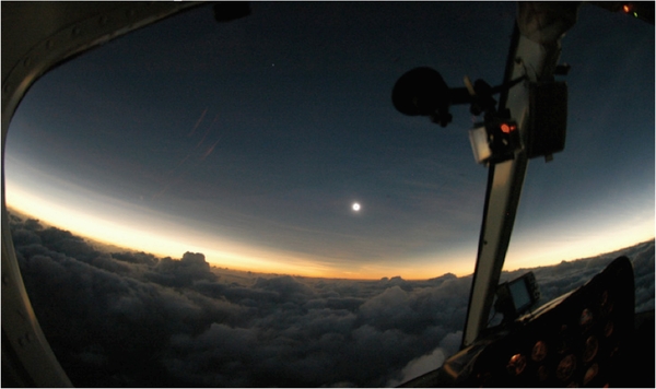
Figure 3. Wide-angle view from a helicopter over Miallo allowed the umbra to be seen racing across clouds; narrow-angle views were also obtained.
Download figure:
Standard image High-resolution image2.3. Coastal Observations
A group of 16 astronomers and astrophysics students from the Aristotle University of Thessaloniki, led by J.H.S. and A.V., with participation from University of Chicago scientist Thanasis Economou, were at an oceanside house at Newell, due east of Miallo. Equipment included a sophisticated spectrograph (constructed by A.V.) for the temperature measurements (Voulgaris et al. 2010, 2012). A satellite site was 20 km north along the coast. Clouds prevented observations from these sites.
Several colleagues had equipment at Trinity Beach, just north of Cairns. People in our group obtained some images through holes in the clouds (Amy Steele, Michael Kentrianakis, Aram Friedman), as well as videos (Friedman 2012) that showed the duration of the clear intervals. Other professional teams, including those of Sterling, of Druckmüller, of Habbal, and of Koutchmy, were in adjacent apartments.
Ten km north along the coast, a meeting of astronomers was held at Palm Cove. A hole in the clouds drifted over their location for totality, and most were fortunate to see the corona then.
2.4. Shipborne Observations
The main set of images with which we compare our Queensland data were obtained by Kazuo Shiota from the Pacific Venus, the second-largest cruise ship (∼800 passengers) registered in Japan. He observed at 21:15 UTC from E 173°4 4 and S 30°22. Though he took 100 images, the ship's rolling limited him to 36 good-quality images in which the corona was fully shown. He also took darks and flats (Figure 4).
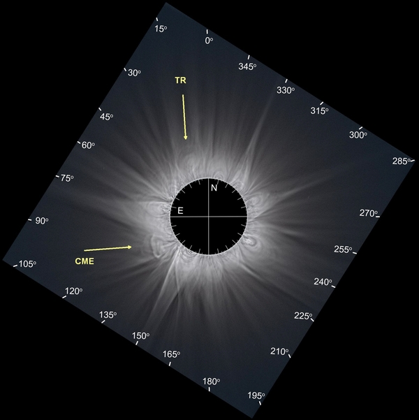
Figure 4.
Combination of 36 white-light corona images, taken by K. Shiota from a ship north of New Zealand, computer-processed by P.G.; solar north, east limb, and position angles (P.A.s) around the solar limb are labeled in white; a CME, not observed in Figure 2, is marked with a yellow arrow; a tennis-racquet-shaped structure is labeled TR. A GIF blinking unlabeled versions of Figures 2 and 4 is available in the Supplemental Material. Hanaoka et al. (2014) have also analyzed a pair of images from this eclipse, which are separated by 35 minutes. (An extended version of this figure is available)
Download figure:
Standard image High-resolution image2.5. Methods of Image Processing
Fifty-eight images from the RED Epic camera on the Tablelands were combined into a composite image that shows the solar-maximum structure of the solar corona shown in Figure 2. Though manual, our reduction method was similar to that used by Druckmüller et al. (2006, 2014), Druckmüller (2009), and Druckmüllerová et al. (2011). Druckmüller's system was unable to handle the REDCODE RAW format of our RED Epic images.
Our basic processing steps were:
- 1.We detected the coordinates of the center of the Moon with high accuracy. The process is automatic and based on mathematical morphology (Petrou & Sevilla 2006).
- 2.We applied a radially graded filter from the center of the Moon to the 58 images. This computer filter removes the steep decrease of brightness of the solar corona and keeps the corona's structure unchanged.
- 3.We aligned the images of step 2 using a phase-correlation method based on two-dimensional Fourier transforms. The accuracy of alignment of the above method is ±0.5 pixels. After this step, we calculated the alignment translations (Δx, Δy) for each image.
- 4.We used the information of step 3 to align the pure (unprocessed) raw images.
- 5.We combined the aligned images. The weights were proportional to the exposure time of each image.
- 6.Finally, we applied locally adaptive filters to enhance the combined image.
3. PROMINENT FEATURES OF THE STRUCTURE OF THE WHITE-LIGHT CORONA
The brightness of the white-light solar corona is a result of Thomson scattering of the photospheric light on free electrons. However, distribution of free electrons is maintained by solar magnetic fieldlines, both local and global, which extend from the photosphere to the solar corona and create different coronal structures. Helmet streamers are the most important streamer type for the brightness distribution; during solar maximum they are nearly uniformly distributed around the solar limb. This type of "corona maxima" has a flattening index below 0.1 and is very rare. The biggest difference in coronal brightness between solar maximum and minimum is around cycle minima, because helmet streamers are then localized only around the solar equator. The flattening index is largest (around 0.3) for such "corona minima." The flattening index is a very simple coronal parameter that shows the overall distribution of magnetic fields with latitude on the Sun. We note that classical helmet streamers are localized above the neutral lines that separate opposite polarities of solar large-scale magnetic fields. The distribution of helmet streamers and their dynamics over the solar-activity cycle was shown by Seagraves et al. (1983) and Bělík et al. (2004).
As a first approximation, the 2012 November 13/14 WLC seen on our combined image can be regarded as the solar-maximum type, with a number of helmet streamers located around the whole solar disk of varying base width and different orientation with increasing height above the surface (Figures 2 and 4), in contrast with the EUV corona (Figure 5).
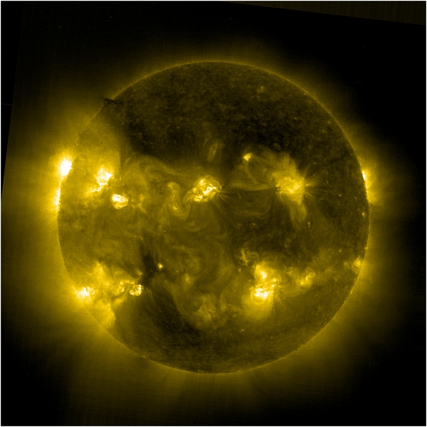
Figure 5. Image of the 284 Å EUV corona (Fe xv, 2 × 10⁶ K), reprocessed by D.B.S. This EUV corona is almost absent in the northern hemiphere at position angles (P.A.s) 295°–45°, even though the white-light corona structures there are well discernible. (Courtesy: ESA/NASA/SOHO/EIT).
Download figure:
Standard image High-resolution imageHabbal et al. (2010a, 2011a, 2011b, 2012, 2013) have also used similarly processed images from the 2006, 2008, and 2010 eclipses as part of their investigation of emission-line ratios and the transition from collisional to collisionless plasma. Habbal et al. (2010b) have reported about such coronal fine structures as prominence shrouds. Habbal et al. (2013) have discussed methods of probing coronal physics with total eclipse observations.
Our images provide the latest value of the flattening index, ε, combining the radial distances, as shown in Figure 6(a), and called Ei (for Equatorial structure) and Pi (for Polar structure):
(Özkan et al. 2007, in their discussion of the 2006 eclipse coronal flattening), which measures the flattening of coronal isophotes at 2 R☉. Our measured value of 0.01 (Figure 6(b)) fits the curve for this phase of roughly 0.07 of the solar-activity cycle (Golub & Pasachoff 2010, and references therein; Figure 6); the graph of the flattening index, shown there in Figure 4.11, was updated based on information from S. Koutchmy (2009, private communication), V. Rušin (2009, private communication), and M. Druckmüller (2009, private communication). It is obvious from Figure 6(b) that the flattening index of the isophotes shown in Figure 6(a) decreases as we move away from the solar limb. This effect reflects the changing structure of the magnetic field of the Sun as a function of the distance away from the photosphere. The flattening index we measure fits well with the phase of the solar-activity cycle (Figure 7).
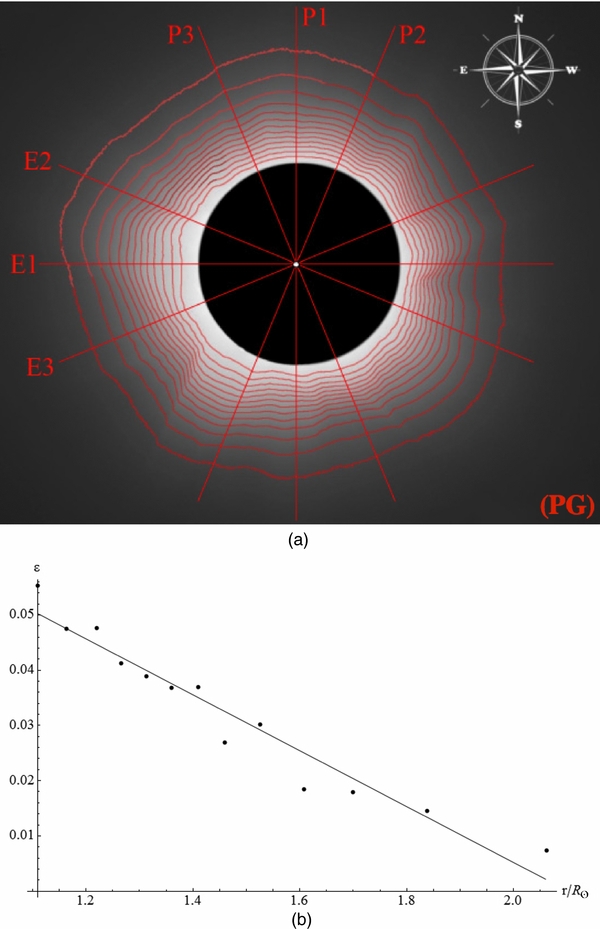
Figure 6. (a) Isophotes superimposed on our composite image. (b) The flattening of isophotes as a function of solar radius.
Download figure:
Standard image High-resolution image
Figure 7. Variation of the flattening index over the phase of the sunspot cycles. Large, red asterisks single out the 2009 and 2010 observations made by the authors' recent publications in this journal, and the 2012 point from the current paper. Even when the magnetic field strength at the solar poles, as measured at Stanford's Wilcox Solar Observatory (http://www.solen.info/solar/polarfields/polar.html), is nearly twice as low compared with previous solar cycles since 1976, the flattening index around cycle maxima has nearly the same value. (Updated and corrected from Golub & Pasachoff 2010; see further analysis of the evolution of coronal flattening in Pishkalo 2011.)
Download figure:
Standard image High-resolution image4. DYNAMICS OF THE WHITE-LIGHT CORONA AT SOLAR MAXIMUM
Thanks to spaceborne observations, short-term changes of small-scale structures of the solar corona have been quite intensively studied lately, e.g., Sheeley et al. (2007), Sheeley & Wang (2007), Moreno-Instertis et al. (2008), and van Ballegooijen et al. (2014). The behavior of large-scale solar coronal structures has been discussed, for example, by Rušin & Rybanský (1984), Koutchmy (1988), Zirker et al. (1992), Pasachoff et al. (2006, 2007, 2008, 2009, 2011a, 2011b), Golub & Pasachoff (2010, 2014), Habbal et al. (2013), and Druckmüller et al. (2014). As the observing sites (Queensland and north of New Zealand) of the images in our comparison were 36 minutes apart in umbral travel time, comparing the corresponding data also enables us to discern interesting changes in the large-scale structure of the WLC on a temporal scale of half an hour. We shall briefly comment on four cases.
The 2012 eclipse fell on a high plateau between the two peaks of cycle 24 (Figure 8): early 2012 and early 2014, according to the mean monthly sunspot number (SILSO, World Data Center—Sunspot Number and Long-term Solar Observations, Royal Observatory of Belgium, on-line Sunspot Number catalog: http://www.sidc.be/silso/dayssnplot). The Sun's level of activity was relatively high, compared to that of the eclipses toward the end of the 23rd cycle, though lower than at other eclipses during sunspot maxima of the past century. Figure 9, which contains both a magnetogram image from Helioseismic Magnetic Imager (HMI) and a 171 Å image from Atmospheric Imaging Assembly (AIA; both on SDO), shows the magnetic-field solar conditions during the eclipse.

Figure 8. Sunspot cycle over the last several decades (cycles 19–24). The lifetimes of selected solar space observatories are indicated with vertical dotted lines. Solar eclipse dates are indicated with letter A to H. TSE stands for total solar eclipse and ASE stands for annular solar eclipse. A: TSE 2006 March 29, B: TSE 2008 August 1, C: TSE 2009 July 22, D: TSE 2010 July 11, E: ASE 2012 May 20, F: TSE 2012 November 13, G: ASE 2013 May 10, and H: TSE 2013 November 3.
Download figure:
Standard image High-resolution image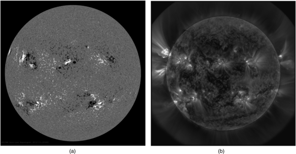
Figure 9. (a) An SDO/HMI magnetogram corresponding to eclipse time in Australia. Terrestrial north is up. (b) An SDO/AIA image at 171 Å showing the high-temperature Fe ix/x corona on the disk, corresponding to eclipse time in Australia. The image has been enhanced with a radial filter. Terrestrial north is up.
Download figure:
Standard image High-resolution imageThe coronal compound images from Queensland and the NZ ship can be understood in terms of the underlying magnetic field. In Figure 10, we see a computed plot of the coronal magnetic-field lines, with source surface (where the magnetic field is constrained to become radial) at heliocentric distance 2.5 R☉, as Wang et al. (2007) described for their similar work at an earlier eclipse (see also Schatten et al. 1969). The extrapolation method is explained in Wang & Sheeley (1992). All field lines that cross the source surface are defined to be "open," with their footpoint areas representing coronal holes. Their calculation used National Solar Observatory/Kitt Peak photospheric field maps for Carrington Rotation (CR) 2129 and CR 2130 (2012 October and November). Mt. Wilson Observatory and Wilcox Solar Observatory photospheric maps gave very similar results (Figure 11). Such Carrington synoptic maps are assembled from central meridian observations taken over the given CR (Figure 12), and reproduced here for long-term reference. The map thus includes data taken both before and after eclipse day. This hairy-ball plot gives a general idea of the topology of the coronal field on November 13/14, showing the locations of coronal holes, helmet streamers separating holes of opposite polarity, and "pseudostreamers" (Wang et al. 2007) separating holes of the same polarity. For a review of the calculations of the Sun's global magnetic field, see Mackay (2012). Habbal et al. (2013) have further discussed linking eclipse observations with determining the structure of the coronal magnetic field while Judge et al. (2013) discuss line-of-sight and other difficulties and properly interpret coronal observations. Alternative calculations by Mikić (2012; "Predictive Science" http://www.predsci.com/corona/nov2012eclipse/nov2012eclipse.html) predicting the coronal appearance were posted prior to the eclipse (Figure 13(a)), allowing verification of the validity of his calculational system according to that usual scientific-method test; see Kramar et al. (2014) for further discussion of the method. The predicted model (Figure 13(b)) was very close to the real state of the WLC. Therefore, such a method should be very useful for modeling the solar corona and forecasting solar wind distribution over a solar cycle. Additionally, the high-resolution WLC images, obtained from ground observations during solar eclipses, remain the best tracers of the global coronal magnetic-field structure.
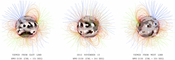
Figure 10. Completed plot of the coronal magnetic-field lines, calculated for a source surface at heliocentric distance 2.5 R☉ by Y. M. Wang (NRL), and viewed from the east, from the Earth, and from the west. Open field lines are depicted in blue (outward-directed) and green (inward-directed), with closed field lines in orange (long loops) and red (short loops).
Download figure:
Standard image High-resolution image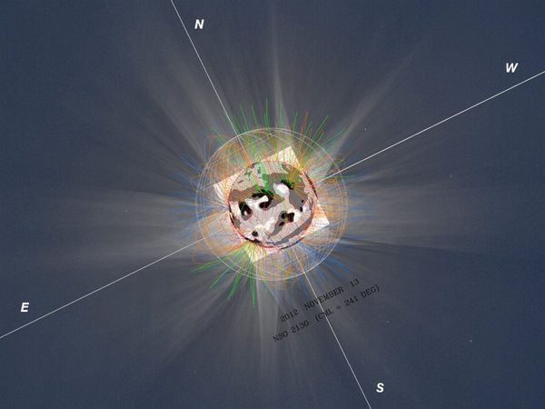
Figure 11. Coronal magnetic-field calculations of Figure 10 overlain on a composite eclipse image by M. Druckmüller made from images by several contributors (http://www.zam.fme.vutbr.cz/~druck/eclipse/Ecl2012a/0-info.htm).
Download figure:
Standard image High-resolution image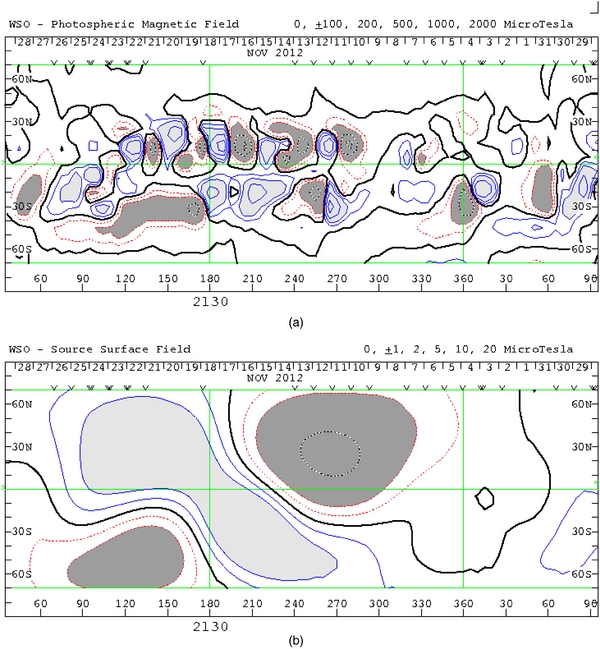
Figure 12. (a) Synoptic charts of the solar magnetic field are assembled from individual magnetograms observed for the CR 2129–2130 graphed for the month centered on the eclipse day. The contour maps show the distribution of magnetic flux over the photosphere. Blue, light shading shows the positive regions (outward field lies). Red, dark shading shows the negative regions (inward field lines). The neutral line is black. (b) The computed Wilcox Solar Observatory coronal magnetic-field map (the source surface at 2.5 solar radii) for the CR 2129–2130 graphed for the month centered on the eclipse day. Blue, light shading shows the positive regions (outward field lies). Red, dark shading shows the negative regions (inward field lines). The neutral line is black. (Courtesy: Todd Hoeksema, Stanford U.)
Download figure:
Standard image High-resolution image
Figure 13. (a) Pre-eclipse prediction of the pB (polarized brightness) coronal structure based on photospheric-magnetic-field data, posted five days before the eclipse by Z. Mikić (Predictive Science). (b) A visual comparison between our group's composite image from the eclipse observation (background) and the predicted coronal magnetic field (overlay with 15% opacity) shows that the model is relatively good. Solar north is 169º counterclockwise from the vertical. Magnetic-field caculations and overlay by Zoran Mikić and Jon Linker, Predictive Science, Inc.
Download figure:
Standard image High-resolution imageWe also compared our images of the WLC with EUV images obtained using the Sun Watcher with Active Pixels and Image Processing (SWAP) onboard ESA's PROBA2 spacecraft (Seaton et al. 2011, 2013; Halain et al. 2013). SWAP images have a passband with its peak at 174 Å and containing the Fe ix/x emission lines that form near 1 million K. To improve the signal-to-noise ratio of the SWAP images at large distances above the solar surface, where the EUV corona is very faint, we generated two composites of 50 10 s images that were obtained during two 60 minute windows surrounding the pair of ground-based eclipse observations. The SWAP composite corresponding to the eclipse observation is shown in Figure 14. To reduce the large dynamic range of the composite, we treated the part of the image outside the limb with a radial filter to remove some of the overall falloff in intensity from the bright inner corona to more extended structures.
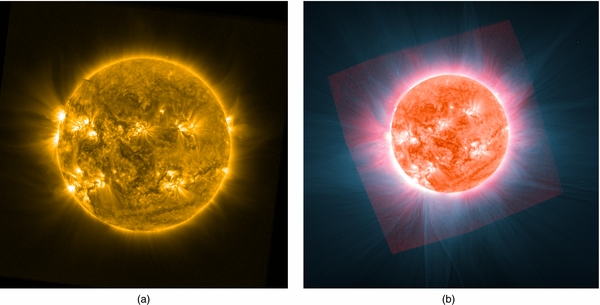
Figure 14. (a) Composite of 50 10 s SWAP images acquired during a 60 minute window surrounding the eclipse observation, showing the full extent of the corona as seen in SWAP's passband, which is centered at 174 Å (0.8–1.0 MK). (b) PROBA2/SWAP composite image of the corona (red), superimposed on a white-light corona image of the Queensland eclipse (blue), showing the on-disk sources of several coronal features. (Courtesy: PROBA2/SWAP Consortium/Royal Observatory Belgium).
Download figure:
Standard image High-resolution imageWhile the SDO/AIA 171 Å passband includes mainly Fe ix with a large contribution from Fe x (Lemen et al. 2011), the PROBA2/SWAP 174 Å passband includes mainly Fe x with a large contribution from Fe ix. Because SWAP's passband is wider than AIA's, it is useful for detecting the flare emission lines of Fe xx and Fe xxiv lines (AIA's passband is therefore dominated by the ∼ MK gas shown by Fe ix/x). The differences among various instrument responses near 171 Å for SOHO/EIT, STEREO/EUVI, SDO/AIA, and PROBA2/SWAP are discussed in Raftery et al. (2013). Habbal et al. (2012) compared the use of such EUV lines with visible-spectrum forbidden emission lines. They found some advantages for the latter as diagnostic tools (when calibrated), with further mention of possible future use of the visible forbidden lines by Judge et al. (2013). We will discuss our forbidden-line spectra from the 2012 and 2013 total solar eclipses in subsequent papers, continuing the series of Voulgaris et al. (2012).
A sample of the AIA images appears in Figure 15; a full set is in the Supplemental Material.

Figure 15.
(a) Spatial distributions of active regions seen in Fe xii at 193 Å, 1,600,000 K. (b) He ii at 304 Å (right) observed with NASA's SDO/AIA at the time of the eclipse. Compare with the HMI image of the magnetic field in Figure 9(a). A full set of SDO/AIA images from close to eclipse time is available in the Supplemental Material. (Courtesy: SDO/LMSAL/NASA). (An extended version of this figure is available.)
Download figure:
Standard image High-resolution image5. COMPARISON OF THE WHITE-LIGHT CORONA WITH SPACEBORNE OBSERVATIONS—A DETAILED TRACING OF A CME
The WLC of the total eclipse of 2012 November 13/14, can aptly and succinctly be described as a highly dynamic and intricately structured corona of maximum type (Figure 16). As mentioned previously, the flattening index, ε, is only 0.01, one of the lowest values on a long-term scale (1851–2010) as studied by Pishkalo (2011). A preliminary estimate of the phase of the 24th cycle (last minimum: 2009; next minimum based on 11 year cycle: 2020) is then 0.37.
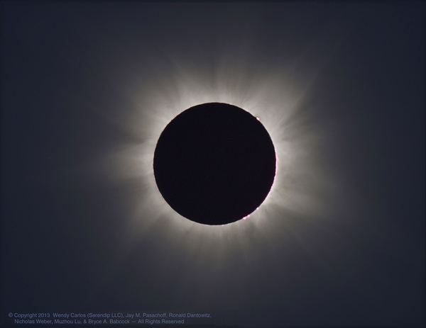
Figure 16. Composite of dozens of our individual images from Mt. Carbine, Queensland, made by Wendy Carlos with less emphasis on contrast than the earlier composites (Figures 2 and 4), but clearly showing the low flattening of this solar-maximum corona.
Download figure:
Standard image High-resolution imageA number of helmet streamers are visible, and some are also well discernible from the Large Angle and Spectrometric Coronagraph Experiment (LASCO) C2 and C3 (Brueckner et al. 1995). They are evenly distributed around the solar disk. Their bases exhibit a great variety of bright and dark loops and arches, with some extending far away from the solar limb, like those located at position angle (P.A.) around 80° and close to 260°. The most pronounced and extended system of helmet streamers is located at P.A.s ranging from 143° to 177°, overlaying a quiescent prominence and a coronal cavity seen in the 284 Å corona (see Figure 5), as well. The increased dynamics of the corona are illustrated by a number of truly spectacular classical CMEs in the period around the time of eclipse. Observations from C2 and C3 reveal a CME on November 12 at 00:12 UTC and at P.A. 300°, a CME on November 13 in the morning at P.A.s 119°–150°, and a couple of CMEs on 14 November, one at 2:24 UTC at P.A. 250° and the other at 12:48 UTC at P.A. 90°. SWAP images show the development of one of the CMEs on the visible disk in the EUV (Figures 17(a) and (b)). Morgan & Habbal (2010b) have discussed distinguishing CMEs from the quiescent corona. Koutchmy et al. (2008) have followed a limb CME outside of an eclipse.
Download figure:
Standard image High-resolution image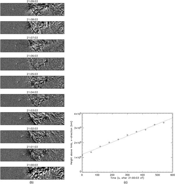
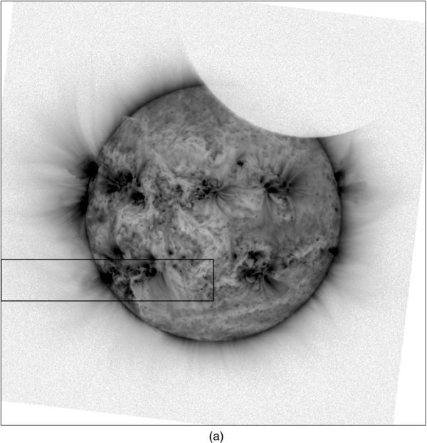
Figure 17. (a) SWAP image taken at UTC 21:02 showing the 174 Å corona. Inverted grayscale is used to enhance contrast, and the narrow box at the SW limb indicates the area sampled for a CME dynamics study (see Figures 17(b) and (c)). (b) A series of SWAP running-difference images showing the evolution of the CME on the disk; the area sampled is enclosed within the box in Figure 17(a). (c) A graph showing the height of the CME above the solar limb over time. The slope of the fitted line shows the average speed of the ejected mass to be 413 km s−1.
Download figure:
Standard image High-resolution imageThe dynamical features of the WLC can be discerned by comparing our eclipse observations from Australia at 20:38 UTC and shipborne observations close to New Zealand (S 30°020, E 173°044) at 21:15 UTC (Figures 18(a) and (b), processed from Figures 2 and 4, respectively). While our observations from Australia show no CME, those made near New Zealand 36 minutes later do show a CME in the interval of P.A.s ranging from 132° to 141°. This CME is rather weak and has a rather complicated shape. Its forerunner, located at about 1.89 R☉ (680,000 km) above the solar limb, is followed by three "legs" emanating from the solar limb at P.A.s 132°, 136°, and 141°. This CME is already seen on the original images at 1.79 R☉ (550,000 km); from C3 this object can still be traced on November 14 at 4:30 UTC at as far as 23 R☉, moving at a speed of 200 km s−1. This particular CME was probably related to a weak flare observed at 21:00:03 with SWAP (Figures 17(a) and (b)), and the speed of the ejected mass was about 413 km s−1 (Figure 17(c)). In the past, such CMEs have probably been mistaken for eclipse comets (e.g., Cliver 1989; Kronk 2003, p.502).
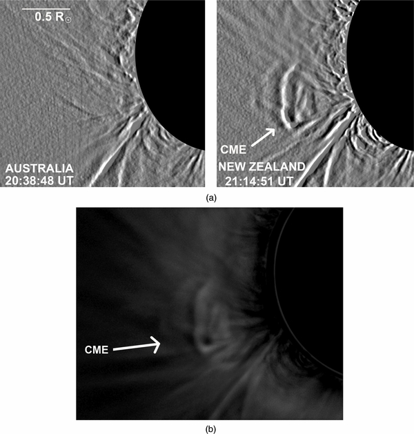
Figure 18. (a) Details of photographs obtained during the total solar eclipse from Mt. Carbine, Australia (left) and from a ship north of New Zealand (right). The time difference between the two photographs is 36 minutes. A CME is not detected in the Australia photograph but is immediately visible in the New Zealand photograph. The photographs were processed using the "Emboss" technique (Kim et al. 2010), a filter that enhances the edges and represents the rate of brightness change. (b) Australia photograph subtracted from the New Zealand photograph (see Figure 18(a)). Differences between the two photographs are, thus, enhanced. A CME is clearly visible, indicating increased activity in this region.
Download figure:
Standard image High-resolution imageIt is worth mentioning that in the period around the eclipse time this particular region exhibited several mass ejections—this one is #65 in ROB's Computer Aided CME Tracking (CACTus); other CMEs associated with this eclipse are #58–70 (see http://sidc.oma.be/cactus/catalog/LASCO/2_5_0/2012/11/latestCMEs.html)—whether in a form of CMEs or propagation of brightening along plumes/arches. Often, as here, CACTus underestimates velocity compared to manual measurements. In this case, the median velocity is decreased by a cluster of slower-moving points at larger P.A.s, but the core of the CME (closer to 90°) is moving faster, which is consistent with our measurements in the lower corona in the EUV.
Another notable object's shape looks like a table-tennis racquet (TR). Its "handle," looking like a screw, is projected from a faint prominence at P.A. 19°. The bottom part of the arc is located at about 250,000 km and the upper part of the arc is at 500,000 km above the solar limb. The highest point of the other loop, located above the described feature, is at 620,000 km, but its legs are rooted at different P.A.s. A comparison of the images taken at 20:38 UTC and 21:14 UTC shows no remarkable changes in its structure. However, observations from C2 (Brueckner et al., 1995) do not show any notable dynamics in this region up to midnight of 2012 November 13. It is also worth noticing a rather intricate complex of features around P.A. 242°. Well-developed dark and bright loops are discernible up to two solar radii, even though a typical helmet streamer is missing. Moreover, these loops seem to be overlaid by faint streamers, easily seen in the ESA's Solar and Heliospheric Observatory (SOHO) corona (see Figures 19 and 20). The orientation of the streamers with respect to the prominences can be seen at Emmanoulidis & Druckmüller (2012).
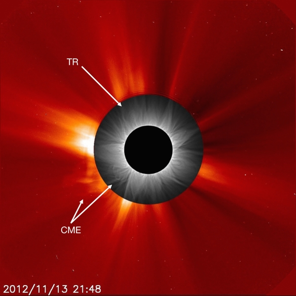
Figure 19. SOHO/LASCO WLC image from the C2 coronagraph (UT 21:48) with our Figure 4 composite (UT 21:15) filling in the middle and inner corona. The same CME, temporally separated by 33 minutes, is labeled; the tennis-racquet-shaped structure (TR) is also visible. (Outer image courtesy: LASCO Consortium/NRL/NASA/ESA; inner image courtesy: NASA's Goddard Space Flight Center/NASA/ESA).
Download figure:
Standard image High-resolution image
Download figure:
Standard image High-resolution image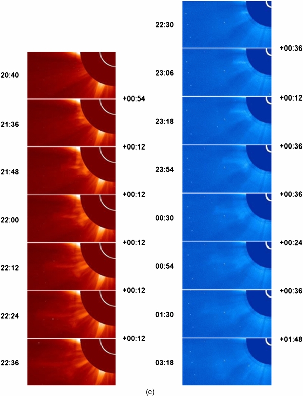
Figure 20. (a) SOHO/LASCO white-light corona image from the C2 coronagraph, with the white circle marking the size and location of the solar photosphere. The selected LASCO images show the CME as it emerges from behind the occulting disk's lower left after the eclipse observations at 20:38 (Australia) and 21:15 (New Zealand ship). (Courtesy: LASCO Consortium/NRL/NASA/ESA). (b) A full SOHO/LASCO C3 image, illustrating the full range of the observed corona during the approximate time of the eclipse, with the CME in the lower left. (Courtesy: LASCO Consortium/NRL/NASA/ESA). (c) Cut-outs of SOHO/LASCO images of the CME. Left: LASCO C2, which images from ∼2–6 R☉; right: LASCO C3, with ∼4 to ∼15–20 R☉. (Courtesy: LASCO Consortium/NRL/NASA/ESA).
Download figure:
Standard image High-resolution image6. DISCUSSION AND CONCLUSION
The composite eclipse images show the structure of the solar corona over the height range of 1–2 solar radii, which is largely unseen from spacecraft equipment. Therefore, they allow us to continuously connect coronal features over a wide range from the solar surface, seen in the UV with AIA and SWAP; through the lower and middle corona that we see at eclipses; and up through the outer corona, which is observed with space coronagraphs. This complete range of observation allows us better to understand the development and location of dynamical structures on the Sun.
Our matched series of highly processed white-light eclipse images from the 2005, 2006, 2008–2010, and 2012 total solar eclipses (Golub & Pasachoff 2014) reveals the diminution of the solar-activity cycle through 2009, its modest resumption by the time of the 2010 total solar eclipse, and the onset of solar maximum by 2012. Morgan & Habbal (2010a) discuss the variations of the outer corona, as seen by LASCO, over the solar cycle. Since we see dynamical changes, we disagree with the conclusion of Woo (2010) that the variations seen in processed images result from differencing rather than actual coronal brightness.
Although activity on the Sun in the current cycle is very low when compared with the several previous cycles, the width of helmet streamers is nearly the same (Rušin et al. 2013). The different distributions of the WLC brightness and the emission in the EUV corona for the northern hemisphere illustrates that different mechanisms are responsible for the WLC and EUV emission corona.
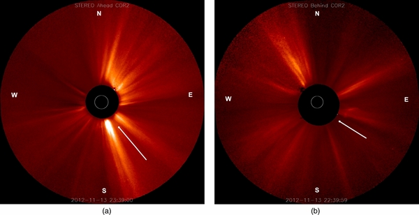
Our composite images from SDO/AIA or SWAP on the disk—through a doughnut of eclipse images—and out through LASCO C2 and C3 allow features to be traced from their on-disk feet (at least for those with feet on the side of the Sun facing us, and the back side of the Sun can now be seen from STEREO) through the eclipse corona and into the outer corona. The magnetic-field structures (Figure 20) correspond well with the our processed eclipse images. STEREO views at that time (Figure 21) provide views of the CMEs from different angles.
Figure 21. (a) STEREO-A's view of the outer corona, with the CME visible as a faint arc slightly below the occulting disk. (b) STEREO-B's view of the outer corona, with the CME visible as an arc to the right of the occulting disk. The arrows in both figures indicate the position of the observed CME, as seen in Figures 17–20. The angle was determined with respect to the bright, southeast helmet streamer. STEREO A and B were separated by 108 6, and were located at 1240 and 1274 from Earth, respectively. (Courtesy: STEREO Science Center).
Download figure:
Standard image High-resolution image
As we discussed in Pasachoff et al. (2011a) and Golub & Pasachoff (2010, 2015), the white-light eclipse images and the SOHO/LASCO images show photospheric light, as scattered by coronal electrons, held in place by unmeasurable coronal magnetic fields. The ultraviolet structures that we see on the solar disk with AIA, EIT, SWAP, or EUVE, on the other hand, show highly ionized coronal ions, directly revealing the high-temperature coronal structures. Our high-resolution composited eclipse observations continue to show many fine-resolution rays similar to those discussed by Wang & Sheeley (2006) and Wang et al. (2007) from the 2006 eclipse.
Theories of coronal heating, including such alternatives as high-frequency waves or nanoflares (recently imaged by High Resolution Coronal Imager), have been summarized by Golub & Pasachoff (2010), among others. De Pontieu et al. (2011) have advanced a coronal-heating theory based on observations of Type II spicules and their energy inputs into the corona. Parnell & De Moortel (2012) have concluded that "the heating of the whole solar atmosphere must be studied as a highly coupled system," with "the dominant mechanisms still undetermined." Van Ballegooijen et al. (2014) have evaluated images of footprints of coronal loops and the relation of their motion to coronal heating in active regions.
The resolution of CMEs in eclipse images is better than the resolution of the images from spacecraft, so total-eclipse observations remain interesting for comparison with the current generation of solar spacecraft. (The proposed PROBA3 spacecraft paired with an occulter hundreds of meters away from the telescope could eventually make possible images that cover the range we can now observe only with eclipses, but that eventuality is years away.) The availability of images from STEREO's two spacecraft, from large angles around the Earth's orbit from Earth-orbiting spacecraft like SDO, allows for three-dimensional calculations of the angles traveled by CMEs (Mierla et al. 2008, 2010).
The eclipse's lunar occultation has an effect on Earth's atmosphere, tracked not only by changes in the clouds after first contact, but also by a drop in temperature, which we normally measure but was somewhat masked at this eclipse by the extensive cloud cover (see, for example, Peñaloza-Murillo & Pasachoff 2015).
The recent observations of the 2013 total solar eclipse from Africa (Pasachoff et al. 2014a, 2014b) will be linked with observations of the 2015 total solar eclipse from the Arctic, including Svalbard, and the 2016 total solar eclipse from Indonesia and the Pacific. These observations will take place as part of the run-up to the 2017 total solar eclipse that will cross the continental U.S. from Oregon to South Carolina, and will be especially valuable not only for scientific considerations but also for public outreach (Hudson et al. 2011; Habbal et al. 2013; Pasachoff 2015).
J.M.P.'s research on the annular and total solar eclipses of 2012 is supported in part by the Solar–Terrestrial Program of the Atmospheric and Geospace Sciences Division of the National Science Foundation through grant AGS–1047726. The 2012 expedition received additional support from the Brandi Fund, the Rob Spring Fund, the Milham Meteorology Fund, and Science Center funds from Williams College. The work of V.R. and M.S. was partially supported by the VEGA grant agency projects 2/0098/10 and 2/0003/13 (Slovak Academy of Sciences) and by NGS Grant 0139–12. For the Australian expedition, we thank Nikon Professional Services and Williams College's Equipment Loan Office/James Lillie for providing equipment. We thank Wendy Carlos for her excellent computer work in providing a composite image of the overall coronal structure based on our imaging. J.M.P. thanks Andy Ingersoll and the Planetary Sciences Department of the California Institute of Technology for their hospitality during the period we composited images and completed the revision. Nicholas Weber of the Dexter Southfield School, Brookline, Massachusetts, was a full participant with the RED Epic cameras and other equipment on site. We also thank Alec Engell of Montana State University and Robert Lucas of the University of Sydney for their helpful participation on site. The assistance of Terry Cuttle of the Queensland Amateur Astronomers was invaluable for finding our sites. For the loan of tracking mounts, we thank Dr. Joe Brimacombe and Dr. Tim Carruthers of Cairns and Charles Frank of Adelaide. Support for D.B.S. and SWAP came from PRODEX grant No. C90345, managed by the European Space Agency in collaboration with the Belgian Federal Science Policy Office (BELSPO) in support of the PROBA2/SWAP mission, and from the European Union's Seventh Framework Programme, Technological Development and Demonstration under grant agreement No. 218816—Project eHeroes (www.eheroes.eu). SWAP is a project of the Centre Spatial de Liège and the Royal Observatory of Belgium funded by the Belgian Federal Science Policy Office (BELSPO). We are grateful for the assistance of David Rust (JHU/APL). We thank Todd Hoeksema of Stanford Solar Observatories Group for providing the Carrington-cycle magnetic-field map. Finally, we are very grateful to Zuzana Kanuchova in Slovakia for help with obtaining and completing the final form of some of the figures.
Facilities: PROBA2 - PRoject for On-Board Autonomy 2 satellite, SDO - Solar Dynamics Observatory, SOHO - Solar Heliospheric Observatory satellite, STEREO - NASA's Solar Terrestrial Relations Observatory