


ABSTRACT
This paper presents a large statistical analysis of  frequency spectra of the solar wind density fluctuations in the range 0.001–5 Hz (corresponding to spatial scales of 100–5 × 10⁵ km). The analysis confirms that the spectrum consists of three segments divided by two breakpoints and that each of the segments can be described by a power-law function with a spectral index α. The first segment corresponds to MHD scales and is followed by a plateau, and the third segment can be associated with the kinetic range. The statistics show that the values of the spectral slopes depend on the density fluctuations; their increasing amplitude leads to a steepening of each segment. The index of −1.8 can typically be found at MHD scales and averaging of the spectra in the frequency domain leads to an index of −8/3 at kinetic scales, whereas averaging in frequencies normalized to the ion gyrostructure frequency, fg, defined as the ratio of the solar wind bulk speed and thermal ion gyroradius, provides a value of −7/3. Both breakpoint locations are controlled by the gyrostructure frequency.
Export citation and abstract BibTeX RIS
1. INTRODUCTION
The solar wind as a weakly collisional plasma (e.g., Kasper et al. 2008) is observed in a turbulent state (Tu & Marsch 1995; Horbury et al. 2005; Matthaeus & Velli 2011; Alexandrova et al. 2013; Bruno & Carbone 2013), and thus it is a unique laboratory to study turbulence in astrophysical plasmas. Measurements of the solar wind turbulent spectra in the vicinity of ion and electron plasma scales may clarify our understanding of the processes of the dissipation (or dispersion) of turbulent energy. Despite many decades of study (e.g., Bruno & Carbone 2013 and references therein), a number of fundamental physical aspects of small scale fluctuations in the solar wind currently remain open questions. In this paper, we examine the shapes and properties of density fluctuations in the transient region between ion and electron scales using an extended statistical set.
In solar wind turbulence, a wide range of scales is predicted and observed: from the fluid regime where the MHD approximation can be used (Biskamp 1993), down to small scales where kinetic effects should be taken into account. The MHD turbulent cascade transports energy from large scales to smaller scales (e.g., Goldstein et al. 1995) until it reaches the ion gyroscale, below which another type of turbulence carries energy to yet smaller scales (Alexandrova et al. 2008; Howes et al. 2008; Sahraoui et al. 2009; Schekochihin et al. 2009; Chen et al. 2010). A typical power-law turbulence spectrum,  (where Pk is the power spectral density at wavenumber k, and α is the spectral index), is present in the region when energy is transferred to small scales, and it is finally dissipated as heat. While in ordinary fluids the dissipation scale is related to the viscosity, in collisionless plasmas, wave–particle interactions are assumed to play the main role in energy dissipation.
At scales below tenths of Hz (at 1 AU), the turbulent energy spectrum of magnetic fluctuations in the spacecraft frame follows a power law with a slope of ≈−5/3 (Kolmogorov 1941), suggestive of a Kolmogorov-like inertial range (Goldstein et al. 1994; Smith et al. 2006) and consistent with a turbulent cascade. The characteristics of turbulence in the dissipation range (i.e., at higher frequencies) are not so well understood; the turbulent magnetic field spectrum follows a steeper power law with a spectral index varying from −2 to −4 (e.g., Leamon et al. 1998; Smith et al. 2006; Alexandrova et al. 2008, 2009; Sahraoui et al. 2009). Recently, the steepening of the spectrum at higher frequencies has been attributed mainly to kinetic Alfvén or Whistler turbulence (Denskat et al. 1983; Goldstein et al. 1994; Leamon et al. 1998; Stawicki et al. 2001; Bale et al. 2005; Galtier 2006; Howes et al. 2008; Sahraoui et al. 2009; Schekochihin et al. 2009; Podesta 2013).
The transition from the MHD scale cascade to small ion scales (≈0.1–0.7 Hz) is often called the ion spectral break. The location of the break in the magnetic field spectrum as well as the physical processes responsible for that break are under debate (e.g., Markovskii et al. 2008; Chen et al. 2014b). Nevertheless, various explanations have been proposed: it coincides with the ion (proton) cyclotron frequency (Denskat et al. 1983; Goldstein et al. 1994; Leamon et al. 1998); it is sensitive to the ion Larmor radius (Leamon et al. 1998; Schekochihin et al. 2009); or it occurs at the ion inertial length (Galtier 2006; Smith et al. 2006).
The spectrum of density fluctuations has been well measured in the inertial range (Intriligator 1975; Neugebauer et al. 1978; Marsch & Tu 1990; Hnat et al. 2005; Podesta & Borovsky 2010), but only a small number of papers have dealt with density fluctuations at the transition to the dissipation range. Between these two ranges before the break, the density spectrum flattens (Neugebauer 1975; Celnikier et al. 1983; Kellogg & Horbury 2005; Chen et al. 2013a, 2014a; Šafránková et al. 2013a) and this flattening has been attributed to the turbulence becoming compressive (Hollweg 1999; Chandran et al. 2009; Chen et al. 2014b) or to pressure anisotropy instabilities (Neugebauer et al. 1978). Chen et al. (2013a) concluded that the shape of the spectrum can be captured by the sum of passive density fluctuations at large scales and kinetic Alfvén turbulence at small scales, and that the whistler fluctuations add only a small portion to the total fluctuation energy (Chen et al. 2013b).
Here, we further investigate the transition between these ranges. Our analysis is based on the ion density data with a time resolution of 32 ms obtained from the Bright Monitor of the Solar Wind (BMSW) on board the Spektr-R spacecraft. The first examples of power density spectra from this monitor were reported by Šafránková et al. (2013a) and by Chen et al. (2014a) and they have shown a spectrum flattening between the inertial and dissipation ranges. We discuss this spectrum flattening near the ion kinetic scale, values of the spectral indices at all scales, and locations of spectral breakpoints using results of a large statistical study in detail.
2. DATA PROCESSING
The determination of solar wind parameters by BMSW is based on measurements of six Faraday cups (FCs). Three of the cups are oriented in different directions with respect to the solar wind velocity and are used to estimate the ion flux vector. The other three FCs point toward the Sun and are equipped with deceleration grids which provide three points for the ion distribution function. These data are sufficient to estimate the ion density, velocity, and temperature (Šafránková et al. 2008, 2013b). The BMSW time resolution allows an analysis of spectral properties up to 16 Hz. However, the present analysis is limited to 8 Hz to avoid the possible influence of instrumental noise on the data (see Šafránková et al. 2013b; Chen et al. 2014a for a detailed noise analysis).
The shape of the frequency spectrum as well as the location(s) of the spectral break(s) would depend on the background (average) magnetic field and plasma parameters. These parameters vary over broad ranges due to the presence of large-scale structures in the solar wind. The studies mentioned in the introduction often used long time intervals (several hours or even more) of the quiet solar wind to obtain sufficient coverage in the frequency domain, but this approach does not allow for the study of disturbed intervals. Since the aim of the present paper is to investigate the shape of the density spectrum in the vicinity of the spectral break dividing the MHD and kinetic scales that can be expected between 0.4 and 4 Hz (Šafránková et al. 2013a; Chen et al. 2014b), we have chosen 20 minute intervals for our frequency spectrum computation. This duration limits our analysis to frequencies above ≈0.001 Hz.
The first power spectrum in a particular interval was calculated over the first 20 minutes. The time span for the calculation of the next spectrum was shifted by 1 minute, and thus two consecutive spectra are overlapped by 19 minutes. The spectra calculated over short intervals are rather noisy and different authors use various routines for their smoothing; a majority of them are based on a calculation of floating mean values or medians. Since we expect a power-law spectrum, we divided an entire frequency interval (0.001–8 Hz) in the logarithmic scale into 100 equal subintervals. The points falling into each subinterval were fitted by a linear fit and the value of this fit corresponding to the interval center was used as the smoothed value. Such a procedure provides the same values as the mean or median but is less sensitive to large dips or spikes. An example of one spectrum is presented in Figure 1(a). The original spectrum is shown as small black dots, whereas the rectangles stand for smoothed values. In order to reflect the expected spectral flattening, the smoothed spectrum was then fit by a combination of three straight lines (in the log–log scale) and two spectral breaks were determined as the frequencies corresponding to intersections of these lines. The fit is shown by the broken red line in Figure 1(a), and the values of slopes as well as the breaks for this particular example are given in the figure together with the slope of −5/3 (blue dashed line).
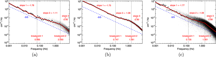
Figure 1. (a) An example of the solar wind density spectrum on 2012 February 6 between 0517 and 0537 UT that defines a terminology used throughout the paper. The original spectrum is shown as small black dots, the rectangles stand for smoothed values. The fit is shown by the broken red line and values of the spectral slopes and breaks are given in the panel. (b) The average frequency spectrum for a whole time interval on 2012 February 6 (between 0100 and 0600 UT). (c) The power density spectrum computed on the same time interval using the classical way (see the text for explanation).
Download figure:
Standard image High-resolution imageWe suggest that the part of the spectrum characterized by Slope 1 can be attributed to MHD turbulence and by Slope 3 to the kinetic range. These two ranges are divided by Breakpoint 2, whereas Slope 2 and Breakpoint 1 characterize the spectral flattening. One may note that Slopes 1 and 3 in Figure 1(a) roughly correspond to their theoretical values but vary in broad ranges within our set. It should be noted that although the fitting procedure works automatically, manual verification of results is needed as about 50% of the spectra exhibit a more complicated pattern (including the foreshock region, magnetic cloud sheaths, interplanetary shocks from different sources, etc) and the procedure cannot treat them properly.
As can be seen in the figure, even smoothed spectra are rather noisy and thus the reliability of the fit is not too high. However, our procedure facilitates a second step of averaging, which is shown in Figure 1(b). This panel presents the average frequency spectrum for a five hour interval in the quiet solar wind. The spectrum corresponds to a time interval from 0100 to 0600 UT on 2012 February 6. This interval was divided into 281 20 minute long intervals overlapped by 19 minutes and the power spectrum of the density fluctuations was calculated in each of them (small black dots). The values of the power density spectrum were then filtered by linear fits as described above (black rectangles) and the smoothed values were fitted (broken red line). One may note a very smooth mean spectrum with well-defined slopes and breaks. In order to compare our averaging procedure with that frequently used, Figure 1(c) presents the power spectrum computed on the same time interval using the classical method, i.e., one frequency spectrum computed over the whole five hour interval that was smoothed and fitted. One may note that the spread of smoothed points around the fit is much lower in panel 1(b) than that in panel 1(c) but the parameters of the fits are nearly identical in both panels. However, if a mean spectrum would be associated with particular values of background parameters, the averaging shown in panel 1(c) requires these parameters to be approximately constant for 5 hr, whereas 20 minutes of constant parameters are sufficient for the averaging demonstrated in panel 1b because the spectra determined on short intervals with the same background parameters can be combined for statistical purposes.
It can be seen that the spectrum has a similar shape to that of the electron density fluctuations (Chen et al. 2012, 2013a), including ion scale flattening (e.g., Celnikier et al. 1983; Chen et al. 2013b), as expected due to quasi-neutrality.
3. STATISTICAL STUDY OF DENSITY FLUCTUATIONS
The parameters of each frequency spectrum (values of slopes and frequencies of breakpoints) were complemented with mean values of magnetic field strength and plasma moments and such a set represents a basic unit for our statistics. As the flux-gate magnetometer does not operate on board Spektr-R, we use the magnetic field data from OMNI by applying a simple time shift, which takes into account the solar wind speed. However, the present study deals with the frequency spectra computed on relatively long time intervals, so possible inaccuracies in the determination of the time shift do not impose notable limitations.
Assuming that the turbulent component of the velocity is much smaller than the bulk speed, the observations can be interpreted as the spatial density variations that are swept past the spacecraft with the bulk speed (Taylor hypothesis). Each particular frequency in the spectrum can thus be associated with a spatial scale. The inertial length,  (where vA is the Alfvén speed and
  is the proton cyclotron frequency) is often considered for scaling of MHD turbulence as well as the thermal gyroradius, RT (
 , where Vth is the most probable speed,
  ). Note that L and RT have been previously suggested to be related to the spectral break between the MHD and kinetic scales (e.g., Galtier 2006; Schekochihin et al. 2009). To check the scaling of breakpoints, we defined an inertial length frequency,
  , where VSW is the solar wind bulk speed, and the gyrostructure frequency
  .
.
Altogether, we obtain 5781 spectra with successfully determined spectral parameters (three slopes of the linear fits and two breakpoints). We investigate the dependence of these 5 spectral parameters on 11 parameters which characterize the solar wind in a given 20 minutes time interval (mean plasma density and its standard deviation, mean solar wind speed and its standard deviation, mean thermal speed and its standard deviation, magnetic field strength, proton gyrofrequency, proton thermal gyroradius calculated using the most probable thermal speed, gyrostructure frequency, and inertial length frequency). All possible combinations of 5 spectral and 11 controlling parameters were verified, and Spearman rank correlation coefficients were calculated for each of them.
The values of correlation coefficients are given in Table 1. We are showing only those quantities for which the magnitude of the correlation with one or more spectral parameters exceeds a value of 0.2. The reliability (standard deviations) of the correlation coefficient determination estimated from a number of points included in the statistics is better than ±0.01. The advantage of the Spearman correlation is that it does not expect any particular functional form of the mutual relations between the two quantities. Nevertheless, the correlation coefficients are generally very low and those exceeding 0.25 are distinguished by bold in the table.
Table 1. Values of Correlation Coefficients between Quantities
| Parameter | n |

|
B | β | fg | fL |
|---|---|---|---|---|---|---|
| Slope 1 | −0.144 | −0.380 | 0.191 | 0.131 | −0.184 | −0.076 |
| Slope 2 | −0.267 | −0.378 | 0.082 | 0.054 | −0.144 | −0.173 |
| Slope 3 | −0.466 | −0.507 | −0.336 | −0.089 | −0.167 | −0.550 |
| Break 1 | 0.151 | 0.208 | 0.291 | −0.143 | 0.256 | 0.171 |
| Break 2 | 0.216 | 0.377 | 0.690 | −0.521 | 0.735 | 0.307 |
| Break 1/Break 2 | −0.009 | 0.047 | 0.213 | 0.249 | 0.285 | 0.040 |
Notes. Values higher than 0.25 are bolded. Parameters are: the ion density, n, density standard deviation,  , magnetic field strength, B, ion β, and gyro-structure and inertial length frequencies, fg and fL, respectively.
Download table as: ASCIITypeset image
Let us concentrate on the spectral slopes first. The table shows notable correlations for all three slopes with a level of the density variations quantified by their standard deviations,  and thus we plot these dependences in Figure 2. Since the spread of the experimental points is very large, we did not fit the data by a curve but divided the whole range into eight equidistantly spaced intervals and computed the median value of the slope on each of them (red solid line). In order to estimate the reliability of such a fit, the first and third quartiles are shown by red dashed lines and the correlation coefficient C is given in the top right corner of each panel.
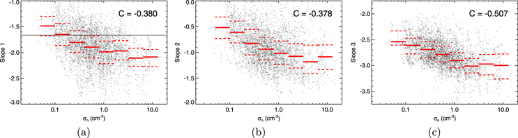
Figure 2. (a), (b), and (c) show Slopes 1, 2, and 3, respectively, as a function of the standard deviation of the density,  . The segments of the thick red line show medians in particular bins; dashed segments stand for first and third quartiles.
Download figure:
Standard image High-resolution imageThe panels demonstrate that all three parts of the spectrum become steeper in a more disturbed flow (larger  ) and this trend is probably saturated at σn ≈ 1–2 cm−3. The steepening of the kinetic part of the spectrum with increasing fluctuation level was also reported by Bruno et al. (2014) for magnetic field fluctuations. Since
  is always lower than the average density, the plot shows that larger slopes are predominantly observed in a dense solar wind and correlations in Table 1 confirm this conclusion. This fact can probably also explain a large correlation of Slope 3 with fL.
Table 1 shows that Breakpoint 2 correlates rather well with all parameters that depend on the magnetic field strength ( ) but the value of the correlation coefficient for fg is the largest one. On the other hand, Breakpoint 1 exhibits the largest correlation with magnetic field strength; the correlation with fg is second. A relatively larger (0.208) correlation with
  suggests that Breakpoint 1 is difficult to associate with a characteristic plasma frequency and more factors come into play.
The breakpoint frequencies are shown in Figure 3 as a function of the gyrostructure frequency. A linear relation between Breakpoint 2 and the gyrostructure frequency could be expected, and Figure 3(b) confirms this expectation (correlation coefficient = 0.735). In order to compare the break in the density spectrum with the break in the magnetic spectrum, we added the results of Bruno & Trenchi (2014) obtained by an analysis of the magnetic field measurements in different distances from the Sun (0.4–5 AU). The gyrostructure frequencies computed from the data given in their Table 1 are shown as green points in Figure 3(b) and they fit very well to the linear trend is distinguished by the blue dotted line that represents the slope of unity. Surprisingly, a similar trend is exhibited by Breakpoint 1 that is well within the MHD range; however, the correlation is rather low in this case. The plots of Breakpoints versus the inertial length frequency exhibit much lower degrees of correlation (0.17 for Breakpoint 1 and 0.31 for Breakpoint 2).
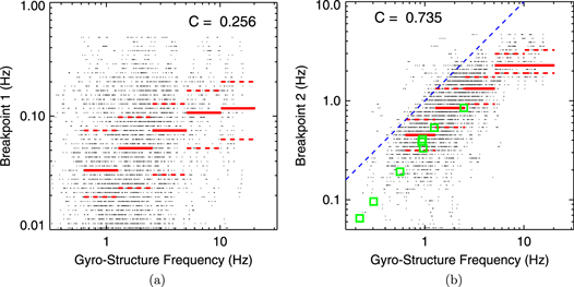
Figure 3. (a) and (b) Breakpoints 1 and 2, respectively, as a function of the gyrostructure frequency. The blue dotted line in panel (b) represents the slope of unity; for an explanation of the green points see the text and for a description of the red lines see Figure 2.
Download figure:
Standard image High-resolution imageAs a next step, we have checked the parameters that control the "width" of the plateau which we describe by the ratio of breakpoint frequencies. The decrease of this ratio with an increasing proton β that is seen in Figure 4(a) is consistent with the suggestions of Chandran et al. (2009). However, we have found that the best organization of this ratio is with the slope of the plateau itself—the steeper the slope, the wider the plateau (Figure 4(b)).

Figure 4. Ratio of Breakpoints 2 and 1 as a function of ion β (a), and a slope of the plateau (b). The segments of the red thick line show medians in particular bins, and the dashed segments stand for first and third quartiles.
Download figure:
Standard image High-resolution imageFigure 5 presents the average slope as a function of the frequency in the spacecraft frame (Figure 5(a)) and the frequency normalized with respect to the gyrostructure frequency, fg (Figure 5(b)) determined as the spacecraft frame frequency divided by fg. The whole set of spectra was split into two halves according to whether fg was larger or smaller than the median. The figures reveal that the mean spectral slope in the MHD range is around −1.9, being slightly steeper for larger gyrostructure frequencies, whereas it is about −2.8 in the kinetic range. These values can be found in the left (right) parts of the figures where only Slope 1 (Slope 3) is averaged. On the other hand, the interval of frequencies between  and 1 Hz (or normalized frequencies between 0.01 and 0.3) is affected by an increasing number of shallow Slopes 2. Since the breakpoint frequencies are correlated with the gyrostructure frequency, the red and blue lines become similar after normalization (Figure 5(b)).
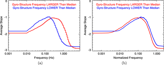
Figure 5. Average slope of the spectrum as a function of the spacecraft frame frequency (a) and normalized frequency (b). The blue (red) line stands for the median slope of spectra computed on intervals where the gyrostructure frequency was below (above) its median value.
Download figure:
Standard image High-resolution imageThe slopes in Figure 5(a) and (b) were obtained as the mean value of the slopes determined individually for each of the  samples. Figure 6(a) and (b) present another approach to the determination of a median solar wind spectrum. The median values of the power spectral density and the corresponding fits to this median spectrum are shown in Figure 6(a). The same procedure was applied to the spectra normalized with respect to the gyrostructure frequency in Figure 6(b). All of the samples were of the same length (38 400 data points), and thus the power spectral densities at individual frequencies are averaged in Figure 6(a). Since the normalization shifts the frequency scales, the medians in the frequency bins are shown in Figure 6(b). The amplitudes of fluctuations in individual samples differ by two orders of magnitude, and thus the power spectral densities in Figure 6(b) were normalized with respect to the total fluctuation power (
 ) prior to calculation of the medians. However, this normalization did not decrease the spread of the points significantly because the separations of the first and third quartiles from the median (three black lines in the figure) are about the same as those in Figure 6(a). It is interesting to note that Slope 3, corresponding to the ion kinetic scale, is −2.63 (close to −8/3) as seen in Figure 6(a), whereas it is −2.37 (i.e., −7/3) when the normalization procedure is applied (Figure 6(b)).

Figure 6. The median power spectral density as a function of the spacecraft frame frequency (a) and normalized frequency (b). The red lines display linear fits, and the values of their slopes are given within the panels. The first and third quartiles are given as scatter estimates.
Download figure:
Standard image High-resolution image
4. DISCUSSION AND CONCLUSION
In the Introduction, we showed that the shape of the frequency spectrum of the solar wind turbulence is a subject of intense debate. For this reason, we have used fast measurements of the ion density on board the Spektr-R spacecraft and carried out a statistical analysis that was concentrated (1) on the slopes of different parts of the density spectrum and (2) on the frequencies corresponding to abrupt changes of spectral indices.
As Figure 1 shows, the frequency spectrum in the range of 0.001–8 Hz can be divided into three parts, and each of them can be fitted by a power-law function. We note that several intervals from our set were analyzed by Chen et al. (2014a) from the point of view of the intermittency of density fluctuations. Although not directly addressed there, the example of the frequency spectrum shown in their Figure 1 exhibits all of the mentioned features. All of the spectral indices in our statistics vary in broad ranges but the inequality Slope 3 < Slope 1 < Slope 2 was fulfilled for each individual spectrum, even though such a condition was not part of our automated fitting procedure. Slope 1, characterizing MHD turbulence, ranges from −1 to −2.5. The value around  that is usually discussed for the MHD regime can be typically found in the undisturbed solar wind (
 cm−3) that was analyzed in a vast majority of published papers (e.g., Malaspina et al. 2010; Chen et al. 2012, 2013b). One possible reason for this spread can be that the value of
  corresponds to the turbulence in an equilibrium between sources and dissipation. When the sources are weak, the frequency spectrum becomes flatter because it tends to reach a fully thermalized state of white noise. This is a situation of a low turbulence level (small
  ). On the other hand, when sources dominate, the turbulent cascade is not efficient enough to dissipate larger structures at a sufficient rate, and thus the slopes become steeper. Studies of turbulence at different distances from the Sun (e.g., Bourouaine et al. 2012; Bruno & Trenchi 2014) implicitly deal with this problem because the fluctuation level decreases by a factor of 10 or more from 0.4 to 1 AU. However, no notable change to the spectral slopes was found over this distance and it suggests that the fluctuation power is only one of the factors influencing the slope of the frequency spectrum.
The analysis of typical slopes (Figure 6) shows that (1) the slope in the proper MHD regime is about −1.8, (2) it ranges from −2.3 to −2.8 in the kinetic regime, and (3) the MHD and kinetic regimes are separated by a plateau with a slope of −1.1. It is interesting to note that the mean slope determined from the averaged spectrum in the kinetic range is  , whereas the physics-based normalization decreases this slope to
  (compare panels in Figures 6(a) and (b)). Both of these values are intensively discussed because each is connected with a specific turbulence model (e.g., Schekochihin et al. 2009; Boldyrev & Perez 2012). However, our statistics show that the slope varies in a broad range, from −2 to −3.5, and different methods of determination of a mean slope provide various results (see Neugebauer 1976 for a discussion of this problem). Moreover, Figure 6 shows the density spectra averaged over a broad range of solar wind conditions and they cannot be considered as representatives of all spectra detected in the solar wind.
The transition between MHD and kinetic scales occurs at Breakpoint 2. Several scaling parameters were suggested for its location in the frequency scale but Figure 3(b) strongly supports the gyrostructure frequency as being the proper scaling parameter. We can conclude that a typical length scale of Breakpoint 2 is  . Bruno & Trenchi (2014) reported that the frequency corresponding to a transition from MHD to kinetic scales (our Breakpoint 2) decreases with the distance from the Sun. However, the magnetic field and ion temperature decrease as well and their break frequencies follow the trend shown in Figure 3(b) despite the fact that their break frequencies were determined from the magnetic field spectra.
A weaker, but non-negligible, correlation of Breakpoint 1 (that divides a true MHD range from the plateau) with the gyrostructure frequency (Figure 3(a)) suggests that the whole frequency range considered would be normalized to this frequency. A smaller correlation is caused by the fact that the location of this breakpoint would also be determined by the proportion of passive scalar and active kinetic Alfvén turbulence (Chandran et al. 2009) as well as ion plasma β. We have plotted the ratio of breakpoints as a function of β in Figure 4(a) and, indeed, the width of the plateau decreases with increasing β as expected. We think that a dependence of the plateau width on its slope (Figure 4(b)) follows from a geometry of fits. However, the physical processes leading to changes of the plateau slope should be investigated. The slope of the plateau determined from the median (normalized) spectrum is −1.18 and −1.13, respectively, which is consistent with the results of Celnikier et al. (1983) and Chen et al. (2013a).
The authors thank the Wind team for the magnetic field data. The BMSW data are available via http://aurora.troja.mff.cuni.cz/spektr-r/project/. This work was supported in part by the project LH14193 financed by the Ministry of Education of the Czech Republic, and in part by the Czech Grant Agency under Contract 209/12/1774, and by the Charles University (under GAUK 1922214). C.H.K.C. was supported by an Imperial College Junior Research Fellowship.
Facilities: Spektr-R -