


ABSTRACT
We report the results of a multiband observing campaign on the famous blazar 3C 279 conducted during a phase of increased activity from 2013 December to 2014 April, including first observations of it with NuSTAR. The γ-ray emission of the source measured by Fermi-LAT showed multiple distinct flares reaching the highest flux level measured in this object since the beginning of the Fermi mission, with  of 10−5 photons cm−2 s−1, and with a flux-doubling time scale as short as 2 hr. The γ-ray spectrum during one of the flares was very hard, with an index of
  , which is rarely seen in flat-spectrum radio quasars. The lack of concurrent optical variability implies a very high Compton dominance parameter
  . Two 1 day NuSTAR observations with accompanying Swift pointings were separated by 2 weeks, probing different levels of source activity. While the 0.5−70 keV X-ray spectrum obtained during the first pointing, and fitted jointly with Swift-XRT is well-described by a simple power law, the second joint observation showed an unusual spectral structure: the spectrum softens by
  at ∼4 keV. Modeling the broadband spectral energy distribution during this flare with the standard synchrotron plus inverse-Compton model requires: (1) the location of the γ-ray emitting region is comparable with the broad-line region radius, (2) a very hard electron energy distribution index
  , (3) total jet power significantly exceeding the accretion-disk luminosity
  , and (4) extremely low jet magnetization with
  . We also find that single-zone models that match the observed γ-ray and optical spectra cannot satisfactorily explain the production of X-ray emission.
Export citation and abstract BibTeX RIS
1. INTRODUCTION
Blazars are active galaxies where the strong, nonthermal electromagnetic emission, generally detected in all observable bands from the radio to γ-ray spectral regimes, is dominated by the relativistic jet pointing close to our line of sight. Detailed studies of blazar spectra, and in particular the spectral variability, are indispensable tools to determine the physical processes responsible for the emission from the jet, leading to understanding the distribution of radiating particles, and eventually, the processes responsible for their acceleration.
3C 279 is among the best studied blazars; it is detected in all accessible spectral bands, revealing highly variable emission. It consistently shows strong γ-ray emission, already clearly detected with the EGRET instrument on the Compton Gamma Ray Observatory (CGRO; Hartman et al. 1992). The object, at z = 0.536 (Lynds et al. 1965), is associated with a luminous flat-spectrum radio quasar (FSRQ) with prominent broad emission lines. Optical and UV observations in the low-flux state (Pian et al. 1999) allow the luminosity of the accretion disk to be estimated at  erg s−1.27
The estimates of the mass of the central black hole are in the range of
erg s−1.27
The estimates of the mass of the central black hole are in the range of  derived from the luminosity of broad optical emission lines (Woo & Urry 2002), the width of the
  line (Gu et al. 2001), and the luminosity of the host galaxy (Nilsson et al. 2009). The object possesses a compact, milliarcsecond-scale radio core and a jet with time-variable structure. Multi-epoch radio observations conducted between 1998 and 2001 by Jorstad et al. (2004, 2005) provided an estimate of the bulk Lorentz factor of the radio-emitting material,
  and the direction of motion to the line of sight,
  degrees, which corresponds to a Doppler factor
  of 24.1 ± 6.5.
As is the case for blazars, the most compelling mechanism for the production of the radio through optical bands is synchrotron emission, while the γ-rays arise via inverse-Compton emission by the same relativistic electrons producing the synchrotron emission (Sikora et al. 2009). Alternative models involving hadronic interactions require significantly higher jet powers due to their lower radiative efficiency (Böttcher et al. 2009). Since in the co-moving frame of the relativistic jet the photon energy density in luminous blazars is dominated by external radiation sources, production of γ-rays is most efficient by scattering of the external photons (Dermer et al. 1992; Sikora et al. 1994). 3C 279 is regularly monitored by the Fermi satellite together with many different facilities covering a range of spectral bands, from radio and optical to X-rays. The correlations of the highly variable time series between the optical polarization level/angle and γ-rays provide strong evidence for the synchrotron + Compton model, and suggest among the solutions that the jet structure is not axisymmetric (Abdo et al. 2010a), or the presence of a helical magnetic field component (Zhang et al. 2015). The rapid variability, together with the rate of change of the polarization angle, suggest a compact (light days) emission region that is located at an appreciable (>a parsec) distance along the jet from the black hole. Furthermore, the close but not exact correlation of the optical and γ-ray flares, with the optical lagging the γ-rays by ∼10 days (Hayashida et al. 2012), has supported this basic scenario (Janiak et al. 2012).
Perhaps the largest mystery in 3C 279—and other luminous blazars as well—is the nature of its X-ray emission (Sikora et al. 2013). Early comparison of the RXTE X-ray and EGRET γ-ray time series revealed a close association of the γ-ray and X-ray flares (Wehrle et al. 1998), suggesting that the X-ray flux might be the low-energy end of the same inverse-Compton emission component detected at higher energies by EGRET. This is supported indirectly by a good overall correlation between long-term RXTE and optical data (which, according to the above, should be a reasonable proxy for γ-ray flux), although individual flares show time lags up to ∼ ±20 days (Chatterjee et al. 2008). However, better sampling provided by the multiband time series covering many years (and owing mainly to the all-sky monitoring capability of the Fermi Large Area Telescope, LAT; Atwood et al. 2009) revealed that the γ-ray and X-ray fluxes are often not well correlated both for this object (Hayashida et al. 2012) and for other blazars (see e.g., Bonning et al. 2009). The nature of blazar X-ray emission is still somewhat unclear.
3C 279 is also a prominent hard X-ray and soft γ-ray source, detected by CGRO/OSSE (Hartman et al. 1996), INTEGRAL (Beckmann et al. 2006), and Swift-BAT (Tueller et al. 2010). However, these observations did not provide a precise measurement of the hard X-ray spectrum of this source that would allow discrimination between alternative spectral components. 3C 279 was selected as one of a few blazar targets to be observed in the early phase of the Nuclear Spectroscopic Telescope Array (NuSTAR; Harrison et al. 2013) focusing hard X-ray (3–79 keV) mission.
After a brief hiatus, 3C 279 became very active late in 2013, producing a series of γ-ray flares and reaching the highest γ-ray flux level recorded by the Fermi-LAT (Buson 2013) for this source. The flaring activities of 3C 279 triggered many observations, including the first two pointings by the NuSTAR satellite, enabling sensitive spectral measurements up to 70 keV. Here, we present the results of the analysis of the Fermi-LAT, NuSTAR, and Swift data together with optical observations by the SMARTS and Kanata telescopes as well as the sub-mm data from the Submillimeter Array (SMA) collected for five months during the high-activity period, from 2013 November to 2014 April. A part of this period—2014 March−April—was studied independently by Paliya et al. (2015). In Section 2 we describe in detail the data analysis procedures and basic observational findings. In Section 3 we compare the observational results between multiple bands. In Section 4 we discuss the interpretation and theoretical implications of our results, and we conclude in Section 5.
2. OBSERVATIONS AND DATA REDUCTION
2.1. Fermi-LAT: Gamma-ray Observations
The LAT is a pair-production telescope on board the Fermi satellite with large effective area ( cm2 on axis for 1 GeV photons) and a large field of view (2.4 sr), sensitive from 20 MeV to 300 GeV (Atwood et al. 2009). Here, we analyzed LAT data for the sky region including 3C 279 following the standard procedure28
, using the LAT analysis software ScienceToolsv9r34v1 with the P7REP_SOURCE_V15 instrument response functions. The azimuthal dependence of the effective area was taken into account for analysis with short time scales (<1 day). Events in the energy range 0.1–300 GeV were extracted within a
cm2 on axis for 1 GeV photons) and a large field of view (2.4 sr), sensitive from 20 MeV to 300 GeV (Atwood et al. 2009). Here, we analyzed LAT data for the sky region including 3C 279 following the standard procedure28
, using the LAT analysis software ScienceToolsv9r34v1 with the P7REP_SOURCE_V15 instrument response functions. The azimuthal dependence of the effective area was taken into account for analysis with short time scales (<1 day). Events in the energy range 0.1–300 GeV were extracted within a  acceptance cone of the Region of Interest (ROI) on the location of 3C 279 (R.A. =
  , decl. =
  , J2000). It is known that the Sun comes very close to and occults 3C 279 on October 8 each year. The data when the source is within
  of the Sun were excluded. Gamma-ray fluxes and spectra were determined by an unbinned maximum likelihood fit with gtlike. We examined the significance of the γ-ray signal from the sources by means of the test statistic (TS) based on the likelihood ratio test.29
The background model included all known γ-ray sources within the ROI from the second Fermi-LAT catalog (2FGL: Nolan et al. 2012). Additionally, the model included the isotropic and Galactic diffuse emission components.30
Flux normalizations for the diffuse and background sources were left free in the fitting procedure.
of the Sun were excluded. Gamma-ray fluxes and spectra were determined by an unbinned maximum likelihood fit with gtlike. We examined the significance of the γ-ray signal from the sources by means of the test statistic (TS) based on the likelihood ratio test.29
The background model included all known γ-ray sources within the ROI from the second Fermi-LAT catalog (2FGL: Nolan et al. 2012). Additionally, the model included the isotropic and Galactic diffuse emission components.30
Flux normalizations for the diffuse and background sources were left free in the fitting procedure.
Several γ-ray light curves as measured by Fermi-LAT can be seen in Figure 1. The top stand-alone panel shows the γ-ray flux above 100 MeV for about 6 years since the beginning of scientific operations of the Fermi-LAT (2008 August 5) up to 2014 August 31 (MJD 54683–56900) binned into 3 day intervals. After ∼MJD 56600, the source entered the most active state since the launch of Fermi satellite. This resulted in target-of-opportunity (ToO) pointing observations for 3C 279, which were performed between 2014 March 31 21:59:47 UTC (MJD 56747.91652) and 2014 April 04 12:42:01 UTC (MJD 56751.52918), and those observations are included in our analysis. The time series of the γ-ray flux and photon index of 3C 279 measured with Fermi-LAT during the most active states from MJD 56615 (2013 November 19) to MJD 56775 (2014 April 28), are illustrated in other panels in Figure 1.

Figure 1. Light curves of 3C 279 in the γ-ray band (integral photon flux) as observed by Fermi-LAT. Top panel shows the long-term light curve above 100 MeV in 3 day bins. The other panels show light curves for the 2013–2014 active period: from the top to bottom, (1) above 100 MeV in 6 hr bins, (2) from 100 MeV to 1 GeV in 1 day bins, (3) above 1 GeV in 1 day bins, (4) arrival time distribution of photons with energies above 10 GeV, and (5) photon index of 3C 279 above 100 MeV in 1 day bins. A gap in the data around ∼MJD 56680–56690 is due to a ToO observation of the Crab Nebula, during which time no exposure was available in the direction of 3C 279. The vertical bars in data points represent 1σ statistical errors and the down arrows indicate 95% confidence level upper limits.
Download figure:
Standard image High-resolution imageThree distinct flaring intervals are evident in the γ-ray light curve: Flare 1 (∼MJD 56650), Flare 2 (∼MJD 56720) and Flare 3 (∼MJD 56750). The maximum 1 day averaged flux above 100 MeV reached 
 (
( ) on MJD 56749 (2014 April 03)31
, which is about three times higher than the maximum 1 day averaged flux recorded during the first two years (on MJD 54800: Hayashida et al. 2012). On the other hand, the maximum 1 day averaged flux above 1 GeV was observed on MJD 56645 (2013 December 20) at
) on MJD 56749 (2014 April 03)31
, which is about three times higher than the maximum 1 day averaged flux recorded during the first two years (on MJD 54800: Hayashida et al. 2012). On the other hand, the maximum 1 day averaged flux above 1 GeV was observed on MJD 56645 (2013 December 20) at 
 , much higher than the
  GeV flux on MJD 56749, which was
 . The photon index also shows a hardening trend toward MJD 56645, when it reached a very hard index of 1.82 ± 0.06, which is rarely observed in FSRQs.
Figure 2 shows detailed light curves around the flares with short time bins. During Flares 1 and 2, the fluxes were derived with an interval of 192 minutes, corresponding to two orbital periods of Fermi-LAT. During Flare 3, because the ToO pointing to 3C 279 increased the exposure, time bins as short as one orbital period (96 minutes) were used. The peak flux above 100 MeV in those time intervals (192 and 96 minutes) reached 
 .
.

Figure 2. Gamma-ray light curves (integral photon flux) of 3C 279 around the three large flares with fine time bins. Top panels: >100 MeV; lower panel: >1 GeV. For Flares 1 and 2, the bins are equal to two Fermi orbital periods (192 minutes). For Flare 3, during a ToO observation, the bins are equal to one Fermi orbital period (96 minutes). The vertical bars in data points represent 1σ statistical errors and the down arrows indicate 95% confidence level upper limits.
Download figure:
Standard image High-resolution imageThe very rapid variability apparent in the data can be fitted by the following function to characterize the time profiles of the source flux variations:

This formula has also been used in variability studies of other LAT-detected bright blazars to characterize the temporal structure of γ-ray light curves (Abdo et al. 2010c). The double exponential form has been applied previously to the light curves of blazars (Valtaoja et al. 1999) as well as gamma-ray bursts(e.g., Norris et al. 2000). In this function, each  and
and  represents the "characteristic" time scale for the rising and falling parts of the light curve, respectively, and t0 describes approximatively the time of the peak (it corresponds to the actual maximum only for symmetric flares). In general, the time of the maximum of a flare (tp) can be described using parameters in Equation (1) as:

The parameters of the fitting results are summarized in Table 1. The time profiles show asymmetric structures in all flares; generally the rise times correspond to 1–2 hr, which are several times shorter than the fall times of 5–8 hr in Flares 1 and 3. On the other hand, the fall time appears to be less than 1 hour in Flare 2 (although the fitting error of the parameter is quite large). One can see in the light curve of Flare 2 in Figure 2 that the flux reached 
 at the peak but suddenly dropped by a factor of ∼3 in the next bin, two orbits (196 minutes) later.
Table 1. Fitting Results of the Light Curve Profile in the γ-ray Band Measured by Fermi-LAT
| Flare |

|

|
b | F0 | t0 |
|---|---|---|---|---|---|
| Number | (hr) | (hr) | (10−7  ) ) |
(10−7  ) ) |
(MJD) |
| Flare 1 | 1.4 ± 0.8 | 7.4 ± 3.2 | 150 ± 36 | 19 ± 12 | 56646.35 ± 0.04 |
| Flare 2 | 6.4 ± 2.4 | 0.68 ± 0.59 | 100 ± 26 | 19 ± 5 | 56718.32 ± 0.07 |
| Flare 3 (ToO) | 2.6 ± 0.6 | 5.0 ± 0.8 | 216 ± 19 | 10.5 ± 6.6 | 56750.30 ± 0.04 |
Download table as: ASCIITypeset image
Gamma-ray spectra were extracted from the following four periods:
- 1.(A) Overlapping with the first NuSTAR observation (see Section 2.2.1). Although the NuSTAR observation lasted for about one day, in order to increase the γ-ray photon statistics, the LAT spectrum was extracted from 3 days where the source showed comparable flux level (as inferred from the light curve with 1 day bins). In this period, the source was found to be in a relatively low state.
- 2.(B) For three orbits (∼4.5 hr) at the peak of Flare 1, when the source showed a very hard γ-ray photon index (<2).
- 3.(C) Overlapping with the second NuSTAR observation (see Section 2.2.1). As in the case of Period A, the length of this period is 3 days, while the NuSTAR observation lasted about 1 day. The source flux was higher than in Period A.
- 4.(D) At the peak of Flare 3 for 4 orbits (∼6 hr).
In a similar manner to previous spectral studies of the source with the Fermi-LAT (Hayashida et al. 2012; Aleksić et al. 2014a), each γ-ray spectrum was modeled using a simple power-law (PL;  ), a broken power-law (BPL;
  for
for  and
and  otherwise), and a log-parabola model (LogP;
  , with
  MeV). The spectral fitting results are summarized in Table 2 and a spectral energy distribution for each period is plotted in Figure 3. In contrast to the general feature of FSRQs that the photon index is almost constant regardless of the source flux (see e.g., Hayashida et al. 2012), the spectral shape significantly changed between the periods. Remarkably, the photon index of the simple PL model for the Period B resulted in an unusually hard index for FSRQs, of 1.71 ± 0.10. Such a hard photon index has not been previously reported in past LAT observations of 3C 279 that included several flaring episodes (Hayashida et al. 2012; Aleksić et al. 2014a). Among the sources in the Second LAT Active Galactic Nucleus (AGN) Catalog (Abdo et al. 2010b), the mean photon index value of FSRQs is 2.4, and only one FSRQ (2FGL J0808.2−0750) in the clean and flux-limited sample has the photon index of
  (see Figure 18 in Abdo et al. 2010b). Occasionally, hard photon indices have been observed in bright FSRQs during rapid flaring events (Pacciani et al. 2014). The photon index of Period B is even harder than the index of 4C + 21.35(1.95 ± 0.21; Aleksić et al. 2011b) and of PKS 1510−089(2.29 ± 0.02; Aleksić et al. 2014b) at the time when the >100 GeV emission was detected.
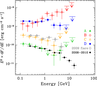
Figure 3. Gamma-ray spectral energy distribution of 3C 279 as measured by Fermi-LAT during the four periods identified in the text (see Section 2.1) as well as in Table 2. The plot includes the spectra of 3C 279 from the 2008–2010 campaign (Hayashida et al. 2012), including a large flare and a 2 years average. In data points, the horizontal bars describe the energy ranges of bins and the vertical bars represent 1σ statistical errors. The down arrows indicate 95% confidence level upper limits.
Download figure:
Standard image High-resolution imageTable 2. Results of Spectral Fitting in the γ-ray Band Measured by Fermi-LAT
| Period | Gamma-ray Spectrum (Fermi-LAT) | Flux ( GeV) GeV) |
# of Photons | |||||
|---|---|---|---|---|---|---|---|---|
| (MJD—56000) | Fitting Modela |

|

|
 (GeV) (GeV) |
TS |
 b
b
|
  ) ) |
 GeV GeV |
| Period A (3 days) | PL | 2.36 ± 0.13 | ⋯ | ⋯ | 174 | ⋯ | 5.9 ± 0.9 | 1 |
| Dec 16, 0 h–19, 0 h | LogP | 2.32 ± 0.17 | 0.03 ± 0.07 | ⋯ | 174 |

|
5.7 ± 0.9 | (26.1 GeV) |
| (642.0–645.0) | ||||||||
| Period B (0.2 days) | PL | 1.71 ± 0.10 | ⋯ | ⋯ | 407 | ⋯ | 117.6 ± 19.7 | 1 |
| Dec 20, 9h36–14h24 | LogP | 1.12 ± 0.31 | 0.19 ± 0.09 | ⋯ | 413 | 6.0 | 94.5 ± 18.1 | (10.4 GeV) |
| (646.4–646.6) | BPL | 1.41 ± 0.17 | 3.01 ± 0.91 | 3.6 ± 1.6 | 415 | 7.6 | 100.6 ± 18.4 | ⋯ |
| Period C (3 days) | PL | 2.29 ± 0.13 | ⋯ | ⋯ | 219 | ⋯ | 17.1 ± 2.8 | 1 |
| Dec 31, 0 h–Jan 03, 0 h | LogP | 2.29 ± 0.16 | 0.00 ± 0.06 | ⋯ | 219 |

|
17.1 ± 2.9 | (14.7 GeV) |
| (657.0–660.0) | BPL | 2.22 ± 0.42 | 2.32 ± 0.20 | 0.34 ± 0.27 | 219 |

|
16.9 ± 3.1 | ⋯ |
| Period D (0.267 days) | PL | 2.16 ± 0.06 | ⋯ | ⋯ | 1839 | ⋯ | 117.9 ± 7.1 | 1 |
| Apr 03, 5h03–11h27 | LogP | 2.02 ± 0.08 | 0.10 ± 0.05 | ⋯ | 1840 | 5.3 | 114.9 ± 7.1 | (13.5 GeV) |
| (750.210–750.477) | BPL | 2.02 ± 0.09 | 2.89 ± 0.45 | 1.6 ± 0.6 | 1843 | 8.0 | 115.1 ± 7.7 | ⋯ |
aPL: power law model, LogP: log-parabola model, BPL: broken-power-law model. See definitions in the text.
b
 represents the difference of the logarithm of the total likelihood of the fit with respect to the case with a PL for the source.
Download table as: ASCIITypeset image
No significant deviations from a PL model were detected in the spectra of Periods A and C, while evidence of spectral curvature was observed in the spectra of the flare peaks, Periods B and D. As derived fitting the BPL model for Period B, the photon index of the lower energy part (below  GeV) is 1.41 ± 0.17. This is comparable to the photon index of the rising part of the inverse-Compton emission for the case of a parent electron index of 2, as is typical of the γ-ray spectra of high-frequency peaked BL Lac objects. One can easily recognize such a rising spectral feature in Figure 3. On the other hand, Period D also shows a very high flux, exceeding 10−5
  (>100 MeV), comparable to the flux of Period B. However, spectral shape is characterized by a soft index (
 ). The photon index of the lower energy part as derived from fitting with the BPL model is not significantly harder than 2, nor is a rising spectral feature apparent in the spectral energy distribution (SED) plot of Figure 3.
2.2. X-Ray Observations
2.2.1. NuSTAR: Hard X-Rays
NuSTAR is a small explorer satellite sensitive to hard X-rays, covering the bandpass of 3–79 keV. It features two multilayer-coated optics, focusing the reflected X-rays onto CdZnTe pixel detectors which provide spectral resolution (FWHM) of 0.4 at 10 keV, increasing to 0.9 at 68 keV. The field of view of each telescope is  , and the half-power diameter of the point spread function is
  . The low background resulting from focusing of X-rays provides an unprecedented sensitivity for measuring fluxes and spectra of celestial sources. For more details, see Harrison et al. (2013).
NuSTAR observed 3C 279 twice. The first observation was performed between 2013 December 16, 05:51:07 and 2013 December 17, 04:06:07 (UTC) and the second one between 2013 December 31, 23:46:07 and 2014 January 01, 22:11:07 (UTC). The raw data products were processed with the NuSTAR Data Analysis Software (NuSTARDAS) package v.1.3.1, using the nupipeline software module which produces calibrated and cleaned event files. We used the calibration files available in the NuSTAR CALDB calibration data base v.20140414. Source and background data were extracted from a region of  radius, centered respectively on the centroid of the X-ray source, and a region 5' N of the source location on the same chip. Spectra were binned in order to over-sample the instrumental resolution by at least a factor of 2.5 and to have a signal-to-noise ratio greater than 4 in each spectral channel. Net "on source" exposure times corresponded to ∼39.6 and ∼42.7 ks for the first (December 16) and second (December 31) observations, respectively. We considered the spectral channels corresponding nominally to the 3.0–70 keV energy range. The net (background subtracted) count rates for the first observation were 0.303 ± 0.003 and 0.294 ± 0.003 cnt s−1 respectively for module A and module B, while for the second observation they were 0.636 ± 0.004 and 0.590 ± 0.004 cnt s−1. We plotted the raw (not background subtracted) counts binned on an orbital time scale in Figure 4. It is apparent that the source was variable from one observation to the other, but also that the source varied within the second observation via secular decrease of flux for the first 3 hr, followed by an increase by nearly a factor of two.

Figure 4. X-ray light curves based on the count rates as measured by NuSTAR (black) and by Swift-XRT (green). NuSTAR data are plotted in 1.5 hr bins, and the Swift-XRT data are plotted for each snapshot. The vertical bars represent 1σ statistical errors.
Download figure:
Standard image High-resolution imageThe spectral fitting was performed using XSPEC v12.8.1 with the standard instrumental response matrices and effective area files derived using the NuSTARDAS software module nuproducts. For each observation, we fitted the two modules simultaneously including a small normalization factor for module B with respect to the module A in the model parameters. We adopted simple PL and a BPL models modified by the effects of the Galactic absorption, corresponding to a column of  cm−2(Kalberla et al. 2005). The results of the two spectral fits were compared against each other by using an F-test to examine improvements by the BPL model. The simple PL model gave acceptable results for both observed spectra, with
  /dof of 666.8/660 (41.9% for the corresponding
  probability) and 831.2/886 (90.6%), respectively. Although the model fluxes in the 2–10 keV band between the two observations showed a difference of about a factor of two, the resulting photon indices were similar: 1.739 ± 0.013, and 1.754 ± 0.008. While there was no improvement in the fit obtained using the BPL model in the first observation, it gave slightly better fits for the spectrum of the second observation, with a
  /dof of 820.8/884 (93.6%), yielding a probability of 0.4% (
 ) that the improvement in the fit was due to chance (as assessed with an F-test). This may indicate a deviation from a single power law in the spectrum of the second observation. The fitting results for the NuSTAR spectra are summarized in Table 3.
Table 3. Parameters of the Spectral Fits in X-ray Band
| Instrument |

|

|

|

|

|
Const. |

|
 /dof /dof |
F-test |
|---|---|---|---|---|---|---|---|---|---|
| (1) | (2) | (keV) (3) | (4) | (keV) (5) | (6) | XRT/module B (7) | (8) | (9) | (prob.) |
| Data on 2013 Dec 16–17 (in Period A) | |||||||||
| Swift-XRT only | 1.67 ± 0.08 | ⋯ | ⋯ | ⋯ | ⋯ | ⋯/⋯ | 11.9 | 21.10/18 (27.4%) | ⋯ |
| NuSTAR only | 1.74 ± 0.01 | ⋯ | ⋯ | ⋯ | ⋯ | ⋯/1.06 ± 0.01 | 11.0 | 666.8/660 (41.9%) | ⋯ |
| XRT + NuSTAR | 1.74 ± 0.01 | ⋯ | ⋯ | ⋯ | ⋯ |

|
11.0 | 688.6/679 (39.1%) | ⋯ |

|
4.5 ± 0.7 | 1.75 ± 0.02 | ⋯ | ⋯ |

|
12.0 | 686.2/677 (39.5%) | 30% (∼1.0 )a )a
|
|
| Data on 2013 Dec 31–2014 Jan 1 (in Period C) | |||||||||
| Swift-XRT only | 1.42 ± 0.03 | ⋯ | ⋯ | ⋯ | ⋯ | ⋯/⋯ | 23.7 | 113.1/109 (37.5%) | ⋯ |
| NuSTAR only | 1.75 ± 0.01 | ⋯ | ⋯ | ⋯ | ⋯ | ⋯/1.00 ± 0.01 | 23.4 | 831.2/886 (90.6%) | ⋯ |
| 1.71 ± 0.02 |

|
1.81 ± 0.02 | ⋯ | ⋯ | ⋯/1.00 ± 0.01 | 23.2 | 820.8/884 (93.6%) | 0.4% (∼2.9 )a )a
|
|
| XRT + NuSTAR | 1.73 ± 0.01 | ⋯ | ⋯ | ⋯ | ⋯ |

|
⋯ | 1072.4/996 (4.6%) | ⋯ |
| 1.37 ± 0.03 | 3.7 ± 0.2 | 1.76 ± 0.01 | ⋯ | ⋯ |

|
22.6 | 940.6/994 (88.6%) | ⋯ | |

|

|
1.72 ± 0.02 |

|
1.81 ± 0.02 | 0.97 ± 0.03/1.00 ± 0.01 | 22.6 | 933.4/992 (90.8%) | 0.22% (∼3.1 )b )b
|
|
| (log parabola)c |
 d
d
|
1 (fixed)e |
 f
f
|
⋯ | ⋯ | 0.90 ± 0.03/1.00 ± 0.01 | 22.7 | 960.6/995 (77.8%) | ⋯ |
Notes. Col. (1) instrument providing the data. Col. (2) photon index for the power law model, or low-energy photon index for the broken-power-law model. Col. (3) break energy (keV) for the broken-power-law model. Col. (4) high-energy photon index for the broken-power-law model. Col. (5) second break energy. Col (6) third index in the double-broken-power-law model. Col. (7) constant factor of Swift-XRT/NuSTAR module-B data with respect to the NuSTAR module-A data. Col. (8) unabsorbed model flux in the 2–10 keV band, in units of 10−12 (erg cm−2 s−1). Col. (9):  degrees of freedom and a corresponding probability.
Download table as: ASCIITypeset image
2.2.2. Swift-X-Ray Telescope (XRT): X-Ray
The publicly available Swift -XRT data in the HEASARC database32
reveal that Swift observed 3C 279 51 times between 2013 November and 2014 April. We analyzed all those observation IDs (ObsIDs). The exposure times ranged from 265 s (ObsID:35019120) to 9470 s (ObsID:35019100). The XRT was used in photon counting mode, and no evidence of pile-up was found. The XRT data were first calibrated and cleaned with standard filtering criteria with the xrtpipeline software module distributed with the XRT Data Analysis Software (version 2.9.2). The calibration files available in the version 20140709 of the Swift-XRT CALDB were used in the data reduction. The source events were extracted from a circular region, 20 pixels (1 pixel  2
2 36) in radius, centered on the source position. The background was determined using data extracted from a circular region, 40 pixels in radius, centered on (R.A., decl.: J2000) = (12h56m26s, −05°49'30''), where no X-ray sources are found. Note that the background contamination is less than 1 % of source flux even in the faint X-ray states of the source. The data were rebinned to have at least 25 counts per bin, and the spectral fitting was performed using the energy range above 0.5 keV using XSPEC v.12.8.1. The Galactic column density was fixed at
  cm−2. The data were analyzed and the flux and photon index were derived separately for each ObsID. A relation between the unabsorbed model flux (0.5–5 keV) and photon index is represented in Figure 5. Only the ObsIDs with an exposure of more than 600 s and with more than 7 spectral points (= dof
  5) were selected for the plot. A trend of a harder spectrum when the source is brighter is clearly detected.

Figure 5. Scatter plot of the X-ray flux (0.5–5 keV) vs. the X-ray photon index  of 3C 279 based on the Swift-XRT data. The horizontal and vertical bars describe 1σ statistical errors for each axis.
Download figure:
Standard image High-resolution imageData with ObsID of 80090001 and 35019132 were taken (quasi-) simultaneously with the NuSTAR observations, and here we report the details of those Swift-XRT observations. The observation with ObsID:80090001 was performed from 2013 December 17 21:06:51 to 22:39:56 (UTC) with an exposure time of 2125 section Therefore, this observation did not exactly overlap with the NuSTAR observation, but it was the closest available, starting about 17 hr after the end of the first NuSTAR observation of the source. The spectral fit with a PL model yielded a photon index of 1.67 ± 0.08 with a flux in the 0.5–5 keV band of 
 .
.
The other observation, with ObsID:35019132, was performed between 2014 January 01 00:20:26 and 22:50:54 (UTC), which overlaps well with the second NuSTAR observation. The exposure time of this Swift observation was 6131 s and the best-fit PL model displayed a photon index of 1.42 ± 0.03 with a flux in the 0.5–5 keV band of 
 . The spectral fitting results are reported in Table 3. Each snapshot observation during this ObsID was also analyzed separately. There were 15 snapshots in total and the exposure time in each snapshot was about 400 s typically, ranging from about 312 s to 594 s. The resultant count rates for all channels are shown in Figure 4.
2.2.3. Joint Spectral Fit of NuSTAR and Swift-XRT Data
Joint spectral fits of the NuSTAR and Swift-XRT data were performed for each NuSTAR observation. As described in previous sections, the data used for the spectral fitting were above 0.5 keV for the Swift-XRT and 3–70 keV for NuSTAR. Here, we introduced a normalization factor of order (1–3)% with respect to NuSTAR module A to account for differences in the absolute flux calibrations, and also to account for the offsets of the NuSTAR and Swift observing times (necessary for an analysis of a variable source). The Galactic column density was fixed at  cm−2 as above. Simple PL, BPL, and double-BPL (for the second observation) models were used for the source spectral models. The joint spectral fitting results are summarized in Table 3.
The joint spectrum during the first NuSTAR observation (December 16) can be represented by a simple power law from 0.5 to 70 keV with a photon index of 1.74 ± 0.01 ( /dof = 688.6/679). The normalization factor of Swift-XRT with respect to NuSTAR module A is 1.01 ± 0.05. The BPL model improved the fit only marginally (
 ) with respect to the PL model. The result indicates that the X-ray spectrum of 3C 279 can be described by a single power law from the soft (0.5 keV) to the hard X-ray (70 keV) band, which is supported by the results from the individual fits for each Swift-XRT and NuSTAR observation alone.
For the joint spectrum during the second NuSTAR observation, the simple PL model did not result in an acceptable fit, with  /dof = 1072/996. Moreover, the normalization factor of Swift-XRT against NuSTAR module A was ∼0.7, which is clearly unacceptable. The BPL model, on the other hand, gave acceptable results with
  /dof = 940.6/994, and the normalization of the Swift-XRT data was 0.97 ± 0.03. The break energy corresponded to 3.7 ± 0.2 keV with photon indices of 1.37 ± 0.03 and 1.76 ± 0.01, respectively, below and above the break energy.
This break energy is located where the bandpasses of Swift-XRT and NuSTAR data overlap, corresponding respectively to the higher and the lower energy end of those data sets. We are confident that the spectral break is a real feature for the following reasons. There is a significant difference in the photon index in each Swift-XRT and NuSTAR data set considered individually. This supports the conclusion that there is a spectral break at an energy close to the overlap of the Swift-XRT and NuSTAR bandpasses. Each resultant individual photon index is similar to the photon index derived from the joint fit below and above the break energy, respectively. The exposures of Swift-XRT and NuSTAR significantly overlapped (see Figure 4), yielding a reasonable inter-calibration constant (0.97 ± 0.03).
We also investigated a double-BPL model. The model yielded a probability of 0.22% ( ) that the improvement in the fit was due to chance against the BPL model as assessed with an F-test. The second break energy appeared at
  keV and the photon index became even softer above the second break energy, changing from 1.72 ± 0.02 to 1.81 ± 0.02. The spectral break at that energy was also seen in the fitting result for the NuSTAR data only at
  keV. All these results suggest that the X-ray spectrum during the high state (the second NuSTAR observation) gradually softens with increasing energy, with the photon index changing by ∼0.4 from ∼0.5 to ∼70 keV. This is the first time that detailed, broadband spectral X-ray measurements of 3C 279 show spectral softening with increasing energy. Furthermore the absence of spectral softening in the first (December 16) NuSTAR observation clearly rules out the spectral shape as being caused by additional absorption. The joint X-ray spectral data points from the soft to the hard X-ray bands obtained by Swift-XRT and NuSTAR are plotted in Figure 6 in the
  (erg
(erg ) form. Finally, a log-parabola model was also tested using the logpar model in XSPEC. The pivot energy was fixed at 1 keV and the best-fit parameters are summarized in Table 3. The model also gave us acceptable fitting results, with
  /dof = 960.6/995.

Figure 6. Spectral energy distributions of 3C 279 in the soft-hard X-ray band based on the combined data from Swift-XRT and NuSTAR. The blue points show the results for observations on 2013 December 16–17 (in Period A), and the red points show the results for observations on 2013 December 31—2014 January 01 (in Period C). The horizontal bars in data points describe the energy ranges of bins while the vertical bars represent 1σ statistical errors.
Download figure:
Standard image High-resolution image2.3. UV–Optical Observations
2.3.1. Swift-UV/Optical Telescope (UVOT): UV Bands
The Swift-UVOT data used in this paper included all observations performed during the time interval from 2013 November to 2014 April. The UVOT telescope cycled through each of the six optical and ultraviolet filters ( ,
,  ,
,  , U, B, V). The UVOT photometric system is described in Poole et al. (2008). Photometry was computed from a 5'' source region around 3C 279 using the publicly available UVOT ftools data-reduction suite. The background region was taken from an annulus with inner and outer radii of
  and
and  , respectively. Galactic extinction for each band in the direction of 3C 279 was adopted as given in Table 4.
Table 4. Galactic Extinctions in the UV–Optical–Near-IR Bands as Used in This Paper
| Band |

|
Instruments |
|---|---|---|

|
0.271 | UVOT |

|
0.285 | UVOT |

|
0.195 | UVOT |
| U | 0.147 | UVOT |
| B | 0.123 | UVOT, SMARTS |
| V | 0.093 | UVOT, SMARTS, Kanata |

|
0.075 | SMARTS, Kanata |
| IC, | 0.056 | Kanata |
| J | 0.027 | SMARTS |
| K | 0.010 | SMARTS |
Notes. The extinctions are based on the reddening of  mag (Schlegel et al. 1998) with
  . See also Larionov et al. (2008)
Download table as: ASCIITypeset image
2.3.2. SMARTS: Optical–Near-IR Bands
The source has been monitored for several years in the optical and near-IR bands (B, V, R, J, and K bands) under the SMARTS project,33
organized by Yale University. Data reduction and analysis are described in Bonning et al. (2012); Chatterjee et al. (2012), and the typical uncertainties for a bright source like 3C 279 are 1%–2%. The publicly available data were provided in magnitude scale. In a similar manner as presented in Nalewajko et al. (2012), the data in magnitude scale  were converted into flux densities as
  , where
  is an effective zero point and
  is the extinction for each band. The effective zero point is calculated as
  , where
  and
and  are parameters taken from Table A2 in Bessell et al. (1998). The extinctions were corrected using the values in Table 4.
2.3.3. The Kanata Telescope: Optical Photopolarimetry
We performed the V-, RC-, and IC-band photometry and RC-band polarimetry observations of 3C 279 using the HOWPol instrument installed on the 1.5 m Kanata telescope located at the Higashi-Hiroshima Observatory, Japan (Kawabata et al. 2008). We obtained 36 daily photometric measurements in each band, and 35 polarimetry measurements in the RC band.
A sequence of photopolarimetric observations consisted of successive exposures at four position angles of a half-wave plate:  ,
,  ,
,  , and
, and  . The data were reduced using standard procedures for CCD photometry. We performed aperture photometry using the APPHOT package in PYRAF,34
and the differential photometry with a comparison star taken in the same frame of 3C 279. The comparison star is located at R.A. = 12:56:14.4 and decl. = −05:46:47.6 (J2000), and its magnitudes are V = 15.92, RC = 15.35 (Bonning et al. 2012) and IC = 14.743 (Zacharias et al. 2009). The data have been corrected for Galactic extinction as summarized in Table 4.
. The data were reduced using standard procedures for CCD photometry. We performed aperture photometry using the APPHOT package in PYRAF,34
and the differential photometry with a comparison star taken in the same frame of 3C 279. The comparison star is located at R.A. = 12:56:14.4 and decl. = −05:46:47.6 (J2000), and its magnitudes are V = 15.92, RC = 15.35 (Bonning et al. 2012) and IC = 14.743 (Zacharias et al. 2009). The data have been corrected for Galactic extinction as summarized in Table 4.
Polarimetry with the HOWPol suffers from large instrumental polarization (δPD ∼ 4%) caused by the reflection of the incident light on the tertiary mirror of the telescope. The instrumental polarization was modeled as a function of the decl. of the object and the hour angle at the observation, and was subtracted from the observed value. We confirmed that the accuracy of instrumental polarization subtraction was better than 0.5% in the RC band using unpolarized standard stars. The polarization angle is defined as usual (measured from north to east), based on calibrations with polarized stars, HD183143 and HD204827 (Schulz & Lenzen 1983). We also confirmed that the systematic error caused by instrumental polarization was smaller than  using the polarized stars.
2.4. Radio Observations
2.4.1. SMA: Millimeter-wave Band
The 230 GHz flux density data was obtained at the SMA, an eight-element interferometer located near the summit of Mauna Kea (Hawaii). 3C 279 is included in an ongoing monitoring program at the SMA to determine the flux densities of compact extragalactic radio sources that can be used as calibrators at millimeter and sub-millimeter wavelengths (Gurwell et al. 2007). Observations of available potential calibrators are from time to time observed for 3–5 minutes, and the measured source signal strength calibrated against known standards, typically solar system objects (Titan, Uranus, Neptune, or Callisto). Data from this program are updated regularly and are available at the SMA website.35
3. MULTI-BAND OBSERVATIONAL RESULTS
3.1. Light Curve
The multiband light curves from the γ-ray to the radio bands taken between MJD 56615 and 56775, are shown in Figure 7 (covering the same period as in Figure 1). The γ-ray light curve measured by Fermi-LAT is plotted using 1 day time bins. The X-ray fluxes were measured by Swift-XRT in the 0.5–5 keV band. The third panel shows fluxes in the optical V-band measured by Swift-UVOT, SMARTS, and Kanata as well as the R-band data measured by SMARTS and Kanata. The optical polarization data were measured by Kanata in the RC-band. The 230 GHz fluxes were based on the results from SMA and also included results by ALMA.36 In the plot, the periods (A–D) as defined in Table 2 are also indicated.

Figure 7. Multiwavelength light curves of 3C 279 covering the same period as in Figure 1. From the top, the panels show: (1) γ-ray photon flux above 100 MeV in 1 day bins from Fermi-LAT; (2) X-ray flux density between 0.5–5 keV from Swift-XRT; (3) optical flux density from Swift-UVOT, SMARTS ( ), and Kanata (V); (4) optical polarization degree (scale on the left) and electric vector polarization angle (EVPA, scale on the right) from Kanata; (5) mm flux density (230 GHz) measured by SMA and ALMA. The vertical dotted lines indicate the periods (A−D) as defined in Table 2 when the γ-ray spectra were extracted. A gap in the γ-ray data by Fermi-LAT around MJD 56680–56690 is due to a ToO observation of the Crab Nebula, during which time no exposure was available in the direction of 3C 279. The vertical bars in data points represent 1σ statistical errors and the down arrows indicate 95% confidence level upper limits.
Download figure:
Standard image High-resolution imageGenerally, the source showed the most active states in the γ-ray band at the beginning (including Period B, Flare 1) and the end (including Period D, Flare 3) of the epoch considered in this paper. In the X-ray band, we also see two high-flux states, in the first half and in the second half of this epoch. While in the first active phase the flux variation was not apparently well correlated between the γ-ray and the X-ray bands, we can see flaring activities in both the γ-ray the X-ray bands around Period D (∼MJD 56750).
During the epoch considered here, the optical flux showed significantly different behavior than that in the γ-ray and the X-ray bands. In the beginning of this epoch, the measured fluxes were relatively low with relatively high polarization degrees, of  . Around period B, the γ-ray showed a very rapid flare with a hard photon index, but the source did not show any enhanced optical fluxes. After that, the optical fluxes started increasing gradually, with a drop of the polarization degree to
  after Period C. The γ-ray and X-ray band fluxes dropped, but the optical flux still continued increasing, and peaked at ~MJD 56720. In the largest flaring event in Period D, where the γ-ray (
 MeV) and X-ray fluxes were highest, the optical flux showed only minor enhancement, and had already started decreasing from its peak value. The optical polarization angle did not show any rotation throughout the observations considered here, and remained rather constant around
  with respect to the jet direction observed by Very Long Baseline Interferometry observations at radio bands (e.g., Jorstad et al. 2005).
The 230 GHz flux was less variable compared with other bands, varying by about 50%, from ∼8 to ∼12 Jy. Even though the amplitude of the variation was much smaller, the general variability pattern of the 230 GHz band followed a similar pattern to that seen in the optical; a low state in the beginning of the epoch, followed by increased activity in the middle, and a decrease toward to the end of the interval. No prominent millimeter-wave flares corresponding to the large γ-ray flaring events (Flares 1–3) were observed.
3.2. Spectral Energy Distributions
Figure 8 shows broadband SEDs for each period as defined in Table 2 (see also Figure 7 in the light curves). The data sets include Fermi-LAT (see also Figure 3), NuSTAR (for Periods A and C), Swift-XRT (for Periods A, C, and D), Swift-UVOT ( for Period A,
  and V for Period C, all six bands for Period D), SMARTS (B, V, R, J, and K bands for all four periods) and Kanata (V, RC bands for Period B), and SMA (for Periods A and C). All data in the figure were taken within the time spans as defined in Table 2, but with a very slight offset in some optical data as follows: for Period B (MJD 56646.4–56646.6), SMARTS data were taken during MJD 56646.348–56646.353 and Kanata data were taken starting at MJD 56646.8078. The SMARTS data observed during MJD 56750.1986–56750.2045 were for Period D (MJD 56750.210–56750.477). Unfortunately, no X-ray observation was performed during Period B. For comparison, the SEDs during a polarization change associated with a γ-ray flare observed in 2009 February, a low state in 2008 August (Hayashida et al. 2012), and very-high-energy γ-ray spectral points measured by MAGIC in 2006 (Albert et al. 2008) are also included.

Figure 8. Broadband spectral energy distributions of 3C 279 for the four observational periods defined in Section 2.1 (see also Table 2 and Figure 7). The vertical bars in data points represent 1σ statistical errors and the down arrows indicate 95% confidence level upper limits. The plot includes historical SEDs of 3C 279 in a low state (in 2008 August) and in a flaring state (in 2009 February) from the 2008–2010 campaign (Hayashida et al. 2012). The measured spectral fluxes by MAGIC in 2006 are also plotted (Albert et al. 2008).
Download figure:
Standard image High-resolution image4. DISCUSSION
This campaign on blazar 3C 279 has three observational results of primary interest: (1) a rapid γ-ray flare with very hard γ-ray spectrum and no optical counterpart observed by Fermi-LAT peaking at MJD 56646 (Flare 1), (2) intraday variability and a stable hard X-ray spectrum observed by NuSTAR in combination with significant X-ray spectral variations observed by Swift-XRT, and (3) a long trend of increasing optical flux without a corresponding increase in the γ-ray flux. These results are discussed in detail in the following subsections.
4.1. Extreme γ-ray Flare
The γ-ray flares peaking at MJD 56646 (Flare 1, Period B) and MJD 56750 (Flare 3, Period D) are the brightest flares detected in 3C 279 by the Fermi-LAT. With photon fluxes of 
 above
above  , they are brighter by a factor
  than the flare peaking at MJD 54880 (Abdo et al. 2010a), and comparable to the record fluxes detected by EGRET (Wehrle et al. 1998).
Flare 1 was characterized by unprecedented rapid variability, with a flux-doubling time scale estimated conservatively at  , and a very hard γ-ray spectrum, with photon index
  . Notably, we do not detect any simultaneous activity in the optical band. These facts make Flare 1 different from any previous γ-ray activity observed in 3C 279. The closest analog was a rapid γ-ray flare in PKS 1510−089 peaking at MJD 55854 with a flux-doubling time scale of
  and photon index of
  (Nalewajko 2013; Saito et al. 2013). However, in that case there were no simultaneous multiwavelength observations because of the proximity of PKS 1510−089 to the Sun.
The SED for Flare 1 is presented in Figures 8 and 9 as Period B. The very hard γ-ray spectrum measured by Fermi-LAT requires that the high-energy SED peak lies at energy  . We assume conservatively the actual SED peak lies at
  , so that the apparent γ-ray peak
  luminosity is
  . We further assume that this γ-ray emission is produced by the external radiation Comptonization (ERC) mechanism (see Sikora et al. 2009 for a review of alternative mechanisms). The corresponding synchrotron component is expected to peak close to the optical band. The observed simultaneous optical/UV spectrum, and the lack of simultaneous optical variability, place very strong constraints on the Compton dominance parameter
  .
.

Figure 9. Top panel: spectral energy distributions of 3C 279 during the brightest γ-ray flares—Flare 1 (Period B, red points) and Flare 3 (Period D, blue points)—see Section 4.1 for discussion. Bottom panel: SEDs during two NuSTAR pointings—Period A (orange points) and Period C (magenta points)—see Section 4.2 for discussion. Solid and dashed lines show SED models obtained with the leptonic code Blazar. Model parameters are listed in Table 5. Black and gray lines show historical data and SED models from Hayashida et al. (2012). Black dashed line shows the composite SED for radio-loud quasars (Elvis et al. 1994) normalized to  . The inset illustrates schematically the decomposition of each SED model into contributions from individual radiative mechanisms: (in order of increasing peak frequency) synchrotron, SSC, ERC(IR), and ERC(BLR). The axes and line types are the same as in the main plot.
Download figure:
Standard image High-resolution imageIn order to constrain the location along the jet r and the Lorentz factor  of the emitting region that produced Flare 1, we use the recent model of Nalewajko et al. (2014). In that model, the allowed parameter space for the γ-ray emitting region is defined by three constraints: (1) a jet collimation constraint
  , where
  is the jet half-opening angle, (2) a constraint on the SSC luminosity
  , where
  is the observed X-ray, hard X-ray, or soft γ-ray luminosity (depending on the expected energy of the SSC peak), and (3) a constraint on the radiative cooling time scale
  , where
  is the characteristic observed energy of the γ-ray photons produced by the electrons for which the radiative cooling time scale is comparable to the variability time scale. The proper size of the emission region is estimated directly from the observed variability time scale
  , and it is related to the jet opening angle by
  . In addition to the parameters discussed above, we adopt a standard ratio of the Doppler-to-Lorentz factors
  , and we also need to specify the upper limit on the expected synchrotron self-Compton (SSC) component. As the SSC component likely peaks in the MeV band, where we do not have any observational constraints, we will conservatively assume that
  . The constraints on the parameter space are shown in Figure 10. The yellow-shaded area indicates the allowed location of the γ-ray emitting region. For reasonable values of the jet Lorentz factor
  , it should be located between
  , where the external radiation is dominated by the broad emission lines (
 ). At larger distances, the energy density of external radiation fields will be insufficient to provide efficient cooling of the electrons producing the
  photons on the observed time scales, and also it will be more difficult to maintain a sufficiently high energy density to power such a luminous γ-ray flare from a very compact emission region. The Lorentz factor should be
  , although this constraint would be stronger if we assumed a lower
  . For the subsequent modeling of the SED, we will adopt two possible solutions indicated in Figure 10: (B1)
  and
and  , and (B2)
  and
and  . This corresponds to the jet opening angle
  satisfying: (B1)
  and (B2)
  .
.

Figure 10. Constraints on the parameter space of location r and Lorentz factor  for the emitting region producing γ-ray Flare 1 (Period B; see Nalewajko et al. 2014, for detailed description of the model). The following constraints are shown: from jet collimation parameter
  (solid red lines), from SSC luminosity
  (dashed blue lines), from energy threshold for efficient cooling
  (dotted magenta line), from the characteristic wavelength of synchrotron self-absorption
  (dotted–dashed orange line), from the minimum required jet power
  (double-dotted–dashed green lines), and from the characteristic energy of intrinsic γ-ray absorption
  (solid gray line). The region allowed by the collimation constraint (
 ), the SSC constraint (
 ) and the cooling constraint (
 ) is shaded in yellow. Two particular solutions B1 and B2 for which SED models are shown in Figure 9 are indicated.
Download figure:
Standard image High-resolution imageWe use the Blazar code (Moderski & Sikora 2003) to model the SED of 3C 279 during Flare 1 with a standard leptonic model including the synchrotron, SSC, and ERC processes. The distribution of external radiation is scaled to the accretion-disk luminosity of  using standard relations for the characteristic radii of the broad-line region (BLR) and the dusty torus (Sikora et al. 2009) with covering factors
  . In general, we use a double-BPL energy distribution of injected electrons
  with two breaks at
  and
and  and three indices: p1 for
  , p2 for
  , and p3 for
  . In order to reproduce a very hard γ-ray spectrum in the fast-cooling regime, we set
  . The goal of the modeling is to match the ERC(BLR) peak with the observed γ-ray peak by adjusting the maximum electron Lorentz factor,
  , and the electron distribution normalization, and then to match the synchrotron component with the optical/UV data by adjusting the co-moving magnetic field B'. One should remember that because of the lack of any optical activity simultaneous with Flare 1, the synchrotron component should actually be below the optical/UV data points, so B' should be treated more like an upper limit than an actual value. The results of the SED modeling are presented in Figure 9, and essential model parameters are listed in Table 5. For solution B1 we obtain
  and
and  , and for solution B2 we obtain
  and
and  .
.
Table 5. Parameters of the SED Models Presented in Figure 9
| Model | A | B1 | B2 | C | D1 | D2 |
|---|---|---|---|---|---|---|

|
1.1 | 0.03 | 0.12 | 1.1 | 0.03 | 1.1 |

|
8.5 | 20 | 30 | 10.5 | 25 | 30 |

|
1 | 0.61 | 0.34 | 1 | 1 | 1 |

|
0.13 | 0.31 | 0.3 | 0.13 | 1.75 | 0.14 |
| p1 | 1 | 1 | 1 | 1 | 1 | 1.6 |

|
1000 | 3700 | 2800 | 1000 | 200 | 100 |
| p2 | 2.4 | 7 | 7 | 2.4 | 2.5 | 2.5 |

|
3000 | ⋯ | ⋯ | 3000 | 2000 | 6000 |
| p3 | 3.5 | ⋯ | ⋯ | 3.5 | 5 | 4 |
Download table as: ASCIITypeset image
We consider the basic energetic requirements for producing such an SED. We can estimate the total required jet power as  , where
  is the radiative efficiency of the jet. And we can use the estimated magnetic field strength to calculate the magnetic jet power
  , where
  is the jet radius,
  is the jet half-opening angle, and
  is the magnetic energy density. For solution B1 we obtain
  and
and  , and for solution B2 we obtain
  and
and  . In both cases, the required magnetic jet power is a tiny fraction of the total jet power. This fraction is higher for solution B2, with
  .This indicates that the emitting region responsible for Flare 1 is very strongly matter-dominated (cf. Janiak et al. 2015), although several observed SEDs of 3C 279 in 2008–2010 can be described by an equipartition model (Dermer et al. 2014).
The total required jet power  appears very high compared with the accretion-disk luminosity
  . For solution B1 we obtain
  , and for solution B2 we obtain
  . We note that there is no signature of increased disk luminosity in the UV data even for the lowest-flux state (Period A), which gives
  . Assuming the black-hole mass of
  (see Section 1), the Eddington luminosity is
  , hence
  and
and  for solution B2. Solution B1 with moderate jet Lorentz factor
  predicts a super-Eddington jet power. The predicted jet power can also be decreased when assuming a higher jet radiative efficiency
  . Taking this into account, the energetic requirements for this flare are consistent with the typical relation between
  and
and  for FSRQs (Ghisellini et al. 2014).
In the standard scenario of magnetic acceleration of relativistic black-hole jets, the jets are initially dominated by the magnetic energy, which is gradually converted into the kinetic energy of plasma until the jet magnetization  (Begelman & Li 1994; Komissarov et al. 2007). Additional conversion of the jet magnetic energy is possible locally under special conditions, e.g., rarefaction acceleration induced by rapid decline in external pressure (Komissarov et al. 2010; Tchekhovskoy et al. 2010; Sapountzis & Vlahakis 2014). However, this additional jet acceleration is likely to lead to the loss of causal contact across the jet, and very wide opening angles (
 ), more typical of gamma-ray bursts. Magnetic energy can be dissipated directly in the process of magnetic reconnection. However, it is unlikely that relativistic reconnection can operate with sufficient efficiency to convert highly magnetized plasma with
  to very weakly magnetized plasma with
  . Additional matter could be injected into the jet by individual massive stars crossing the jet (Khangulyan et al. 2013), or at the jet base during a brief pause in the jet production (Dexter et al. 2014). The latter possibility potentially allows for a more uniform distribution of an unmagnetized plasma layer across the jet.
The very hard electron energy distribution with  extending up to
  , required to explain the very hard γ-ray spectrum of Flare 1, is challenging for many particle acceleration mechanism and emission scenarios (e.g., Blandford & Levinson 1995). Very hard electron spectra can be obtained in relativistic magnetic reconnection, but they require extremely high electron magnetization
  (Guo et al. 2014; Sironi & Spitkovsky 2014; Werner et al. 2014). In the case of an electron–proton jet composition with no
  pairs, one has
  , where
  and
and  are typical Lorentz factors of protons and electrons, respectively. In principle, it is possible that
  , so that such extreme acceleration of electrons is possible even in the case of
  . The final outcome of the acceleration depends on how the dissipated magnetic energy is shared between the protons and electrons; the first study of relativistic electron–ion reconnection suggests roughly equal energy division (Melzani et al. 2014).
We propose that Flare 1 of 3C 279, together with the similar flare of PKS 1510−089 peaking at MJD 55854 (Saito et al. 2013), constitute an emerging class of rapid γ-ray events characterized by flux-doubling time scales of a couple of hours, very hard γ-ray spectra with spectral peaks in the GeV band, and significant time asymmetry with longer decay time scales (Nalewajko 2013). Moreover, the results of this work indicate that such events do not have significant multiwavelength counterparts. Since only two clear examples were identified in bright blazars during ∼6 years so far of the Fermi mission, they appear to be rare events, and may not represent typical conditions of dissipation and particle acceleration in blazar jets.
In Figure 9, we also present two SED models for Flare 3 (Period D). This flare is characterized by a typical γ-ray spectrum, and a more typical Compton dominance, as compared to Flare 1. In addition, for Flare 3 we have simultaneous UV and X-ray data from Swift. The soft X-ray spectrum is very hard, with  . We first attempted—in model D1 located in the BLR—to explain this X-ray spectrum by SSC emission from a very hard electron energy distribution (
 ). By coincidence, model B1 described in the previous subsection does exactly that. However, since the γ-ray spectrum for Period D is much softer than the exceptionally hard γ-ray spectrum for Period B, in model D1 we need to adopt a break in the electron energy distribution at
  , which shifts the observed peak of the SSC component to
  ; hence the X-ray part of the SSC spectrum is too soft to explain the observed X-ray spectrum. We note that Paliya et al. (2015) present an SED model for a period overlapping with our Period D, in which the X-ray spectrum is matched with the SSC component. They made the model by adopting a higher value of
  , which requires a superposition of ERC(BLR) and ERC(IR) components to explain the γ-ray spectrum. In model D2 we were able to explain the X-ray spectrum with the low-energy tail of the ERC emission. The emission region in model D2 is located outside the BLR, and the entire high-energy component is strongly dominated by the ERC(IR) emission. We adopted a higher jet Lorentz factor
  and the low-energy electron distribution index
  for
for  (see Table 5). While model D2 matches the observed X-ray spectrum, because it is located at relatively large distance
  , it predicts a rather long observed variability time scale of
  .
.
Such extremely high-flux spectra as observed in Periods B and D could in some cases extend to even higher energies, and may possibly be detectable by ground-based Cherenkov telescopes (MAGIC, H.E.S.S., VERITAS, CTA). Despite its moderate redshift, 3C 279 was detected twice by MAGIC (Albert et al. 2008; Aleksić et al. 2011a) before the Fermi era. In this work, we have argued that the γ-rays originate at a radius  , which is comparable with the estimated size of the broad emission line region
  based upon reverberation mapping campaigns of other AGNs (e.g., Bentz et al. 2006; Kaspi et al. 2007). This radius is also roughly comparable to the minimum radius from which the highest energy photon observed during our campaign—
 (
( in the quasar rest frame) in Period A—can escape without pair production. The highest energy photons detected in Periods B and D were
  and
and  , respectively (see Figure 1). We could not distinguish whether the non-detection of
  photons was due to the absorption by the BLR photons or just the statistical limitation of the short integration time for the spectra. Our emission models indicate a sharp drop in the source intrinsic spectral shape at
  energies due to adopting a very steep high-energy electron distribution index
  . In addition, the γ-ray emission above
  produced in the ERC(BLR) process is suppressed due to the reduction of the scattering cross section in the Klein–Nishina regime.
The importance of γ-ray absorption in the pair-production process depends on the abundance of soft photons produced in the jet environment. One source of soft photons is the emission lines radiated by the broad emission line clouds. The optical depth depends on the geometrical shape of the BLR, and is significantly reduced for the flat geometries (Tavecchio & Ghisellini 2012; Stern & Poutanen 2014). Specifically, the results of Tavecchio & Ghisellini (2012) calculated for  and for an intermediate geometric case indicate that absorption from BLR photons is not significant for γ-ray photons with
  emitted at
  , and those with
  at
at  . However, other models of the BLR can be expected to set a larger lower bound on the emission distance scale r. Another source of soft photons is Thomson scattering by the hot inter-cloud medium that is commonly invoked to confine the clouds by ram pressure. If we adopt the spectral component associated with the accretion disk by Pian et al. (1999), then the radius of the "γ-sphere" (for the
  photons in the source frame) is
  , where
  is the mean Thomson depth (e.g., Blandford & Levinson 1995).
The difficulties faced by the leptonic models do not necessarily mean that they should be abandoned, unless there exists a better alternative. Hadronic models have been applied to 3C 279 (Böttcher et al. 2009; Petropoulou & Mastichiadis 2012; Diltz et al. 2015); however, they always require an extremely large jet power of order  , which is difficult to reconcile with observations of radio galaxies and theories of jet launching (Zdziarski & Boettcher 2015).
4.2. Spectral Variability in X-Ray and Hard X-Ray Bands
The X-ray and hard X-ray behavior of 3C 279 revealed by Swift-XRT and NuSTAR appears to be quite complex. This is especially interesting since the origin of this emission in FSRQ-type blazars is in general controversial and poorly understood (Sikora et al. 2013). Here, we focus on constraining the mechanism of X-ray and hard X-ray emission observed during the two NuSTAR pointings (Periods A and C).
The X-ray flux observed during the NuSTAR pointings is relatively high for 3C 279, higher by a factor of ∼5 than typical X-ray fluxes measured during the 2008–2010 campaign (Hayashida et al. 2012). In Period C, the X-ray flux is higher by a factor of ∼2 than in Period A, and it also shows some intraday variations. A comparison of the broadband SEDs for Periods A and C suggests a roughly linear relation between optical, X-ray, and γ-ray variations; however, this may be misleading, as the optical flux shows a long-term systematic increase that is not evident in the X-ray and γ-ray light curves. With typical photon index  , the observed X-ray spectrum is relatively hard, with a spectral break observed in Period C at
  . The Swift-XRT data show a clear anti-correlation between the soft X-ray photon index and the soft X-ray flux (see Figure 5).
The X-ray emission of FSRQs is typically attributed either to the SSC emission of medium-energy electrons or to the ERC emission of low-energy electrons. Adopting a one-zone model in the SSC scenario for the X-ray band, we attempted to explain the observed broadband SEDs for Periods A and C together with the synchrotron emission for the optical band and the ERC component for the γ-ray band. Figure 9 shows the SEDs for Periods A and C with the emission models based on the parameters in Table 5. Actually, the observed high X-ray flux and hard X-ray spectra challenge the SSC scenario. In order to match the relatively high observed X-ray luminosity with that expected to be produced via SSC, as well as the corresponding synchrotron component and the ERC components with a condition of  , one needs to adopt a rather low jet Lorentz factor
  for Period A and
  for Period C. A low jet Lorentz factor requires a more powerful jet; in the case of Period C with γ-ray luminosity
  we estimate
  . The jet Lorentz factor can be higher, and the required jet power lower, by allowing that
  . Typical X-ray SEDs from the SSC component in FSRQs are flat; it is possible to obtain a hard SSC spectrum by choosing an electron energy distribution peaking at
  . However, in order to reproduce apparent linear relations between optical, X-ray, and γ-ray fluxes from Periods A to C, it was necessary to adjust the value of
  to compensate for the quadratic dependence of the SSC luminosity on the synchrotron luminosity
  . Therefore, while it is possible to make a one-zone model that fits the observed SEDs for both Periods A and C with X-rays produced by the SSC process and with reasonable jet power, such a model cannot naturally account for the observed flux variations over the multiwavelength bands. We note that lower Lorentz factors
  required for modeling the SEDs for Periods A and C, together higher Lorentz factors
  required for modeling the SEDs for Periods B and D, could indicate the existence of a spine-sheath jet structure (Ghisellini et al. 2005). In such case the γ-ray flares would be produced in the fast spine and the bulk of X-ray and hard X-ray emission in the slow sheath.
In the ERC scenario, on the other hand, the observed X-ray flux could be dominated by the low-energy tail of either the ERC(BLR) or ERC(IR) components, depending on the location of the emitting region. In one-zone models, this would require the X-ray spectra to be related to the γ-ray spectra by a single spectral component. This would explain the apparent linear relation between the X-ray and γ-ray data, although there are insufficient X-ray observations in the current campaign to probe the direct correlation between X-ray and γ-ray fluxes. (During the previous campaign on 3C 279, no significant correlation was detected between the X-ray and γ-ray fluxes; Hayashida et al. 2012). Judging from the simultaneous X-ray, hard X-ray and γ-ray SEDs, it could be possible to connect them by a single spectral component, especially for Period A. This would require a PL extension of the X-ray spectrum all the way to the low-energy end of the γ-ray spectrum. This is possible only for the ERC(IR) component where no cooling break is expected. However, because the low-energy ERC(IR) emission would be produced deep in the slow-cooling regime, very little flux variability would be expected on daily time scales. The ERC(BLR) component is very likely to feature a cooling break, and possibly an additional low-energy spectral break at  produced by trans-relativistic electrons (
 ).
).
We conclude that there is no one-zone leptonic SED model that can satisfactorily explain the production of X-ray emission observed by NuSTAR in 3C 279. Various alternative mechanisms can be proposed where the observed X-ray emission is produced at a different location from the optical and/or γ-ray emission. Observation of a transient spectral break at  in Period C may indicate a superposition of two spectral components in the X-ray band. Similar spectral breaks observed in high-redshift FSRQs were interpreted as due to very strong absorption (Fabian et al. 2001); however, in our case this interpretation is challenged by the lack of a break in Period A, only two weeks earlier. Alternative mechanisms for the X-ray emission include IC emission from the accretion-disk corona, ERC, or synchrotron emission from the jet acceleration region, and hadronic mechanisms (Böttcher et al. 2009). However, for most mechanisms it may be challenging to explain the relatively high X-ray luminosity
  observed during Period C, a factor ∼3 higher than
  . This certainly excludes the accretion-disk coronal emission proposed tentatively for PKS 1510−089 in the low state (Nalewajko et al. 2012). The "jet base" scenario, where luminous weakly beamed X-ray emission is produced at very short distances from the supermassive black hole at which the jet is not yet fully accelerated, is motivated by recent observations of misaligned FSRQs (Bostrom et al. 2014), and will be investigated in detail elsewhere.
4.3. Optical Behavior
The observed optical flux shows a systematic increase by a factor of ∼4 over a period of ∼80 days (MJD 56645–56725). Superposed on this trend are weak flares that correspond very poorly to the strong γ-ray flares. No similar systematic trend is seen in the X-ray and γ-ray light curves. This is in contrast with the good overall correlation between optical and γ-ray fluxes in 2008–2010 (Hayashida et al. 2012). The lack of overall correlation between the optical light curve and the radio (mm-band), X-ray, and γ-ray light curves suggests that they are produced by different populations of electrons, and most likely at different locations. Moreover, the apparent linear relation between SEDs for Periods A and C is merely a coincidence. As the overall radiative output from 3C 279 is always dominated by the γ-ray emission, the systematic long-term increase in the optical flux could be due to a systematic increase of the magnetic field strength, or a systematic decrease of the external radiation energy density. The former option would be problematic if the jet magnetization remains constant, which would lead to an increase in the total jet power, and ultimately to an increase in the γ-ray luminosity, which is not observed.
5. CONCLUSIONS
We report the results of observations of the well-studied γ-ray luminous blazar 3C 279 at the end of 2013 and beginning of 2014, when the object entered a bright and active state. The Fermi-LAT observations revealed multiple distinct, bright flares, and recorded the highest γ-ray flux state of the source since the launch of Fermi, at  reaching 10−5 photons cm−2 s−1 on 2013 December 20 and 2014 April 03. The high flux of the source allowed us to integrate the γ-ray flux on time scales as short as one Fermi-LAT orbit (96 minutes). This in turn allowed us to establish the variability time scales to be as short as
  hr. One of these flares revealed an unprecedentedly hard γ-ray spectrum, with a photon index
  , unusual for this kind of source.
Two NuSTAR observations provided the first precise measurement of the hard X-ray spectrum of 3C 279 up to 70 keV. The NuSTAR observations were complemented by more frequent Swift observations. The best-fit model for the joint spectra by NuSTAR and Swift-XRT during the first NuSTAR observation (2013 December 16) was consistent with a simple power law, which usually has been observed in past X-ray observations involving Suzaku and XMM-Newton (Hayashida et al. 2012). On the other hand, the second simultaneous NuSTAR and Swift observations at the end of 2013 revealed a spectral structure that was harder ( ) below
  and softer (
 ) above that energy. Such a spectral structure has not been observed in 3C 279 in any previous X-ray observations. In addition, the second NuSTAR observation (2013 December 31) indicated an increase of the X-ray flux by ∼50% during the 1 day pointing. In the soft X-ray data from Swift-XRT, we found a clear correlation between the flux and photon index with a harder-when-brighter trend. More detailed studies offer potential for better understanding of the origin of X-ray emission in FSRQ blazars.
The optical flux of the source steadily increased since the beginning of this multiwavelength campaign, but did not show clear, large-amplitude flares such as those seen in γ-rays. The optical flux of the source does not appear clearly correlated with the γ-ray flux, in contrast to the behavior measured in 2008–2010 (Hayashida et al. 2012). It is possible that the optical flux might be arising in multiple locations along the jet, as expected if the electrons radiating in the optical are of different energy than those making the X- and γ-rays, which is suggested by the apparent lack of correlation between the optical flux and the optical polarization degree.
We modeled the broadband spectrum of the source at multiple epochs, including two very bright γ-ray flares, and the two NuSTAR pointings. The very hard γ-ray spectrum and very high Compton dominance during the first γ-ray flare are very challenging to explain in the standard one-zone synchrotron plus SSC/ERC model, requiring electron energy distribution index  , a high jet power compared to the accretion-disk luminosity
  , and a very low magnetic fraction of the jet power
  . In addition, no single-zone modeling of any single epoch of the broadband SED can satisfactorily explain the production of X-ray emission at the same time as it explains the optical and γ-ray emission. This conclusion is consistent with the finding that variations in the X-ray flux of 3C 279 are not always simultaneous with variations in the γ-ray or optical fluxes.
The Fermi-LAT Collaboration acknowledges generous ongoing support from a number of agencies and institutes that have supported both the development and the operation of the LAT as well as scientific data analysis. These include the National Aeronautics and Space Administration and the Department of Energy in the United States; the Commissariat à l'Energie Atomique and the Centre National de la Recherche Scientifique/Institut National de Physique Nucléaire et de Physique des Particules in France; the Agenzia Spaziale Italiana and the Istituto Nazionale di Fisica Nucleare in Italy; the Ministry of Education, Culture, Sports, Science and Technology (MEXT), High Energy Accelerator Research Organization (KEK) and Japan Aerospace Exploration Agency (JAXA) in Japan; and the K. A. Wallenberg Foundation, the Swedish Research Council, and the Swedish National Space Board in Sweden. Additional support for science analysis during the operations phase is gratefully acknowledged from the Istituto Nazionale di Astrofisica in Italy and the Centre National d'Études Spatiales in France.
This work was partially supported under the NASA contract no. NNG08FD60C, and made use of observations from the NuSTAR mission, a project led by California Institute of Technology, managed by the Jet Propulsion Laboratory, and funded by NASA. We thank the NuSTAR Operations, Software, and Calibration teams for support of the execution and analysis of these observations. This research has made use of the NuSTAR Data Analysis Software (NuSTARDAS) jointly developed by the ASI Science Data Center (ASDC, Italy) and the California Institute of Technology (USA). This research has made use of the XRT Data Analysis Software (XRTDAS) developed under the responsibility of the ASI Science Data Center (ASDC), Italy. The Submillimeter Array is a joint project between the Smithsonian Astrophysical Observatory and the Academia Sinica Institute of Astronomy and Astrophysics and is funded by the Smithsonian Institution and the Academia Sinica.
K.N. was supported by NASA through Einstein Postdoctoral Fellowship grant number PF3–140130 awarded by the Chandra X-ray Center, which is operated by the Smithsonian Astrophysical Observatory for NASA under contract NAS8–03060. M.B. acknowledges support from NASA Headquarters under the NASA earth and Space Science Fellowship Program, grant NNX14AQ07H.
Facilities: Fermi (LAT) - Fermi Gamma-Ray Space Telescope (formerly GLAST), NuSTAR - The NuSTAR (Nuclear Spectroscopic Telescope Array) mission, Swift - Swift Gamma-Ray Burst Mission, CTIO: 0.9m - , CTIO: 1.0m - , CTIO: 1.3m - , CTIO: 1.5m - , SMA - SubMillimeter Array
Footnotes
- 27
- 28
- 29
TS = 25 with 2 degrees of freedom (dof) corresponds to an estimated
 pre-trials statistical significance assuming that the null-hypothesis TS distribution follows a distribution (see Mattox et al. 1996).
 - 30
iso_source_v05.txt and gll_iem_v05_rev1.fit
- 31
Throughout this paper, each error represents a
statistical uncertainty. - 32
- 33
- 34
PYRAF is a product of the Space Telescope Science Institute, which is operated by AURA for NASA. See http://www.stsci.edu/institute/software_hardware/pyraf.
- 35
- 36
Taken from the ALMA Calibrator Catalog, https://almascience.eso.org/sc/.


