


ABSTRACT
Interstellar dust grains produce X-ray halos around bright sources due to small-angle X-ray scattering. Numerous studies have examined these halos, but no systematic study has yet tested the available halo data against the large number of well-defined dust models in circulation. We have therefore obtained the largest sample to date of X-ray dust halos from XMM-Newton and Chandra, and fitted them with 14 commonly used dust grain models, including comparisons with the optical extinction, AV, where available in the literature. Our main conclusions are summarized as follows. (1) Comparing AV with NH values measured via X-ray spectral fits, we find a ratio of AV/NH (1021 cm−2) = 0.48 ± 0.06, in agreement with previous work. (2) Out of 35 halos, 27 could be fit by one or more grain models, with the most successful models having maximum grain radius  μm and fewer large grains than the less successful models. This suggests that the diffuse ISM does not contain a signicant presence of grains with
  μm. (3) Most halos were best fit assuming a single dust cloud dominated the scattering, rather than smoothly distributed dust along the sightline. (4) Eight sources could not be fit with the models considered here, most of which were along distant (
 kpc) sight lines through the Galactic thin disk. (5) Some sight lines had halos with observed X-ray scattering optical depth τsca/AV that were signicantly different than expected. This may result from an inhomogeneous dust distribution across the halo extraction area.
Export citation and abstract BibTeX RIS
1. INTRODUCTION
Modern X-ray observations have opened a new window onto the study of interstellar (IS) dust grains, especially the largest grains that contain most of the refractory metals in the Galaxy. X-rays, like all other photons, may be either absorbed or scattered by intervening gas and dust along the line of sight (LOS). X-rays typically pass through grains and thus X-ray absorption measurements are directly sensitive to dust porosity, composition, and mantles. X-rays can also undergo small-angle scattering by dust, with a cross section that increases rapidly with dust size (Overbeck 1965; Mathis & Lee 1991). As we detail here, these properties provide us with a new view of IS dust.
In combination with constraints from more standard approaches in the optical, ultraviolet (UV), and infrared (IR), X-ray measurements can reveal otherwise hidden properties of IS dust. Currently, IS dust models are observationally constrained primarily by their interactions with UV and optical light and by their IR emission. These observations measure the composition, shape, and size distribution of the dust up to radii of about 0.1 μm, above which they begin to behave as undifferentiated gray particles. Halos around X-ray sources created by IS dust open a new window on the properties of the large particles that provide the dominant fraction of dust mass and otherwise have no observational manifestation.
IS dust models must characterize the composition, morphology, and size distribution of the various particles, but must also fix the abundances, relative to hydrogen, of the elements in the dust. There are a number of viable dust models that can explain the various astrophysical phenomena associated with the presence of dust in the ISM, such as the wavelength dependence of the IS extinction, scattering, polarization, IR emission, and depletion pattern of the different elements. Our current dilemma is not a paucity but an abundance of dust models that fit most of the existing data reasonably well (Zubko et al. 2004, hereafter ZDA). It is not a coincidence that the biggest problem for most dust models—meeting the existing abundance constraints—coincides with the lack of observational constraints on the large grains that have most of the mass.
To address this problem, we present a survey of energy-resolved X-ray halos taken from the HEASARC archive, which were extracted and analyzed using a uniform methodology. Earlier surveys have been done with the ROSAT archive by Predehl & Schmitt (1995), but the 29 sources they selected from the ROSAT archive were chosen primarily due to an expectation of a strong halo, and so focused on highly absorbed X-ray binaries. Our approach was somewhat different: we focused on sources that were less heavily absorbed, but in many cases with known values of optical extinction AV; our selection approach is discussed in detail in Section 3.
While the underlying grain model strongly affects the observed X-ray halo, other astrophysical and instrumental impacts also affect the observations. The position of the dust along the LOS has purely geometrical effects on the shape of the resulting halo (see Figure 1). Separating the effect of dust position from the intrinsic dust composition and size distribution is made significantly easier if the halo can be measured at multiple energies. ROSAT's detectors lacked energy sensitivity, which meant that most of the Predehl & Schmitt (1995) survey results could only fit their halos assuming the dust was evenly distributed along the LOS. Thus Chandra and XMM-Newton results have an advantage, which we use here to show that most lines of sight are dominated by dust at a single position, possibly with a background of smoothly distributed dust or dust in one other cloud. Given our knowledge of molecular cloud distribution in the Galaxy, this result is not a surprise.
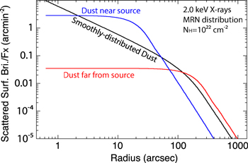
Figure 1. Theoretical dust scattering curves for dust near the source, near the observer, or smoothly distributed between the source and observer.
Download figure:
Standard image High-resolution imageCrowding and background were also major effects for the survey. The excellent angular resolution provided by Chandra 's mirror is useful here, but since halos are generally of arcminute-scale, a low background is even more important to detect the halo out to the largest scales. In this, ROSAT has the advantage due both to its orbit and its detector technology; both Chandra and XMM-Newton have much higher backgrounds that limit our halo measurements to much smaller angular distances than were used in the Predehl & Schmitt (1995) survey. The mirror point-spread function (PSF) must also be carefully measured. As discussed in Smith et al. (2002), this must be specially calibrated directly from observations because micro-roughness dominates the mirror scatter at large angles and this is not well determined by ray-trace models.
2. METHOD
Scattering by IS dust grains creates most of the extinction (scattering plus absorption) observed at optical and UV wavelengths, which is typically characterized by  , the magnitude of the extinction in the V band. The number density of grains in the ISM, especially in the Galactic plane, ensures that optical and UV light can only be detected out to relatively short distance. Small angle scattering of X-rays by dust grains in the ISM, however, has a less immediate effect. Unlike optical/UV scattering, the small-angle nature of the scattering does not eliminate all emission, but rather creates an arcminute-scale halo around the source.
Overbeck (1965) first discussed X-ray halos in an astrophysical context; since then a number of authors have elaborated upon the theory (Mauche & Gorenstein 1986; Mathis & Lee 1991; Smith & Dwek 1998). In his detailed review of X-ray scattering, Draine (2003) used a phenomenological approach to define the dust halo scattering "optical depth." Starting with that,we define the total number of photons from a source (at energy E) to be  , then we can define the optical depth for scattering,
  , via the equation
  , which gives (from Draine 2003 Equation (20), with a typographical error corrected here)

Values of  can be directly calculated for any given energy assuming a dust model, the LOS distribution, and a model for the grain scattering itself. The fundamental quantity is the differential scattering cross section
  , which can be calculated using either the exact Mie solution or the Rayleigh–Gans (RG) approximation (see Smith & Dwek 1998 for a discussion). By integrating the dust size distribution and the scattering cross section over the LOS geometry (and considering single scatterings only), we get the halo surface brightness (relative to the source flux F(E)) at angle θ from the source:

where NH is the hydrogen column density, S(E) is the (normalized) X-ray spectrum, and  is the dust grain size distribution (in which n(a) is normalized to NH and a is the radius of a spherical grain). Here f(x) is the density of hydrogen at distance xD from the observer divided by the LOS average density, assuming D is the distance to the source (Mathis & Lee 1991). Considering only single scatterings, the total number of scattered halo photons between suitable angles
  and
and  can be determined via

Table 1 presents values of τsca for each dust model under consideration for both a smooth distribution and single-cloud values at two characteristic energies, 1.5 and 2.5 keV, plus the model of Witt et al. (2001; hereafter WSD). These calculations were done using exact RG theory combined with realistic optical constants from Draine (2003). Ratios for energies larger than 2.5 keV can be extrapolated assuming an  decay, following RG theory; energies below 1.5 keV require a full Mie treatment, which is beyond the scope of this paper. These calculations include all scattering angles out to 30 arcmin, although, except in ideal conditions, X-ray halos can be detected only between ∼30 and 600 arcsec, so these values are also presented in the table. For the purposes of these calculations, we used NH/A
 cm2 mag−1, which agrees with our work presented in Section 5.2 (NH/A
  cm2 mag−1), so we believe that this is reasonable.
Table 1. Observable X-ray Halo Scattering τsca per Unit Optical Extinction (AV) both Integrated over all Angles and Limited to Scattering Between θ = 30 and 600 arcsec for a Range of Dust Models and Distributions at Two Characteristic Energies
| Model | 1.5 keV (All Angles) | 2.5 keV (All Angles) | 1.5 keV (30''–600'') | 2.5 keV (30''–600'') | ||||||||
|---|---|---|---|---|---|---|---|---|---|---|---|---|
| x = 0.1 | Smooth | x = 0.9 | x = 0.1 | Smooth | x = 0.9 | x = 0.1 | Smooth | x = 0.9 | x = 0.1 | Smooth | x = 0.9 | |
| MRN | 0.0272 | 0.0275 | 0.0282 | 0.0103 | 0.0102 | 0.0103 | 0.0226 | 0.0220 | 0.0151 | 0.0092 | 0.0078 | 0.0030 |
| WD | 0.0400 | 0.0397 | 0.0402 | 0.0150 | 0.0146 | 0.0146 | 0.0353 | 0.0315 | 0.0161 | 0.0137 | 0.0106 | 0.0028 |
| WSD | 0.1776 | 0.1624 | 0.1265 | 0.0683 | 0.0585 | 0.0303 | 0.1157 | 0.0639 | 0.0074 | 0.0265 | 0.0133 | 0.0013 |
| ZBGS | 0.0239 | 0.0241 | 0.0247 | 0.0091 | 0.0090 | 0.0091 | 0.0196 | 0.0193 | 0.0136 | 0.0081 | 0.0069 | 0.0028 |
| ZBGF | 0.0246 | 0.0248 | 0.0254 | 0.0093 | 0.0092 | 0.0093 | 0.0203 | 0.0198 | 0.0136 | 0.0084 | 0.0071 | 0.0028 |
| ZBGB | 0.0190 | 0.0193 | 0.0198 | 0.0072 | 0.0071 | 0.0072 | 0.0148 | 0.0153 | 0.0123 | 0.0063 | 0.0056 | 0.0027 |
| ZBAS | 0.0251 | 0.0251 | 0.0256 | 0.0095 | 0.0093 | 0.0094 | 0.0215 | 0.0204 | 0.0127 | 0.0087 | 0.0071 | 0.0023 |
| ZBAF | 0.0256 | 0.0255 | 0.0261 | 0.0097 | 0.0095 | 0.0096 | 0.0220 | 0.0207 | 0.0128 | 0.0089 | 0.0072 | 0.0023 |
| ZBAB | 0.0199 | 0.0200 | 0.0205 | 0.0075 | 0.0074 | 0.0075 | 0.0164 | 0.0162 | 0.0117 | 0.0068 | 0.0058 | 0.0023 |
| ZCGS | 0.0296 | 0.0293 | 0.0297 | 0.0110 | 0.0107 | 0.0106 | 0.0264 | 0.0229 | 0.0106 | 0.0100 | 0.0076 | 0.0018 |
| ZCGF | 0.0274 | 0.0273 | 0.0277 | 0.0102 | 0.0100 | 0.0100 | 0.0241 | 0.0217 | 0.0112 | 0.0093 | 0.0073 | 0.0020 |
| ZCGB | 0.0217 | 0.0218 | 0.0222 | 0.0080 | 0.0079 | 0.0079 | 0.0183 | 0.0174 | 0.0111 | 0.0072 | 0.0060 | 0.0021 |
| ZCAS | 0.0243 | 0.0239 | 0.0242 | 0.0089 | 0.0086 | 0.0085 | 0.0220 | 0.0184 | 0.0073 | 0.0080 | 0.0058 | 0.0012 |
| ZCAF | 0.0224 | 0.0222 | 0.0225 | 0.0082 | 0.0080 | 0.0080 | 0.0201 | 0.0175 | 0.0079 | 0.0075 | 0.0057 | 0.0013 |
| ZCAB | 0.0142 | 0.0141 | 0.0143 | 0.0051 | 0.0049 | 0.0049 | 0.0127 | 0.0108 | 0.0045 | 0.0045 | 0.0033 | 0.0008 |
| ZCNS | 0.0056 | 0.0056 | 0.0058 | 0.0021 | 0.0021 | 0.0022 | 0.0049 | 0.0046 | 0.0027 | 0.0020 | 0.0016 | 0.0005 |
| ZCNF | 0.0207 | 0.0204 | 0.0206 | 0.0074 | 0.0071 | 0.0070 | 0.0189 | 0.0155 | 0.0056 | 0.0066 | 0.0047 | 0.0009 |
| ZCNB | 0.0169 | 0.0166 | 0.0168 | 0.0060 | 0.0057 | 0.0056 | 0.0155 | 0.0125 | 0.0039 | 0.0053 | 0.0037 | 0.0007 |
Download table as: ASCIITypeset image
We briefly review the characteristics of the various dust models considered herein. We used the models of Mathis et al. (1977; hereafter MRN), Weingartner & Draine (2001; hereafter WD), and Zubko et al. (2004; hereafter ZDA). These models assume a ratio of total to selective visual extinction RV = 3.1, which is the standard Galactic value. RV in the Galaxy ranges from 2.5 to 5.5, with denser sight lines having higher values, likely due to grain growth (Cardelli et al. 1989).
MRN presented a dust model consisting of populations of spherical graphite and silicate grains in a power law (PL) distribution with size cutoffs at 50 Å and 0.25 μm.
WD presented a wide range of dust models; we used their model with  (Case A) and
  as our standard case for WD, but present calculations for the full range of models in Table 2. In addition to modeling sight lines with RV = 3.1, WD also provided models for RV = 4.0 and 5.5.
Table 2. Total X-ray Halo Scattering τsca per Unit Optical Extinction (AV) for the WD Models and Distributions at Two Characteristic Energies
| RV | b
|
1.5 keV (All Angles) | 2.5 keV (All Angles) | 1.5 keV (30''–600'') | 2.5 keV (30''–600'') | ||||||||
|---|---|---|---|---|---|---|---|---|---|---|---|---|---|
| 105 | x = 0.1 | Smooth | x = 0.9 | x = 0.1 | Smooth | x = 0.9 | x = 0.1 | Smooth | x = 0.9 | x = 0.1 | Smooth | x = 0.9 | |
| 3.1(A) | 0.0 | 0.0391 | 0.0389 | 0.0394 | 0.0147 | 0.0143 | 0.0142 | 0.0338 | 0.0304 | 0.0165 | 0.0131 | 0.0103 | 0.0031 |
| 3.1(A) | 1.0 | 0.0393 | 0.0391 | 0.0396 | 0.0148 | 0.0144 | 0.0143 | 0.0340 | 0.0306 | 0.0165 | 0.0132 | 0.0103 | 0.0031 |
| 3.1(A) | 2.0 | 0.0393 | 0.0390 | 0.0395 | 0.0148 | 0.0144 | 0.0143 | 0.0341 | 0.0306 | 0.0165 | 0.0132 | 0.0104 | 0.0031 |
| 3.1(A) | 3.0 | 0.0393 | 0.0391 | 0.0396 | 0.0148 | 0.0144 | 0.0143 | 0.0342 | 0.0308 | 0.0165 | 0.0133 | 0.0104 | 0.0031 |
| 3.1(A) | 4.0 | 0.0395 | 0.0393 | 0.0398 | 0.0149 | 0.0145 | 0.0144 | 0.0346 | 0.0310 | 0.0163 | 0.0134 | 0.0105 | 0.0029 |
| 3.1(A) | 5.0 | 0.0398 | 0.0395 | 0.0400 | 0.0149 | 0.0146 | 0.0145 | 0.0349 | 0.0313 | 0.0163 | 0.0135 | 0.0106 | 0.0029 |
| 3.1(A) | 6.0 | 0.0400 | 0.0397 | 0.0402 | 0.0150 | 0.0146 | 0.0146 | 0.0353 | 0.0315 | 0.0161 | 0.0137 | 0.0106 | 0.0028 |
| 4.0(A) | 0.0 | 0.0519 | 0.0510 | 0.0511 | 0.0195 | 0.0188 | 0.0182 | 0.0463 | 0.0390 | 0.0165 | 0.0172 | 0.0127 | 0.0027 |
| 4.0(A) | 1.0 | 0.0517 | 0.0508 | 0.0510 | 0.0194 | 0.0187 | 0.0182 | 0.0463 | 0.0391 | 0.0164 | 0.0172 | 0.0127 | 0.0027 |
| 4.0(A) | 2.0 | 0.0512 | 0.0504 | 0.0507 | 0.0192 | 0.0186 | 0.0182 | 0.0461 | 0.0391 | 0.0165 | 0.0172 | 0.0128 | 0.0027 |
| 4.0(A) | 3.0 | 0.0511 | 0.0504 | 0.0507 | 0.0192 | 0.0186 | 0.0183 | 0.0462 | 0.0394 | 0.0165 | 0.0173 | 0.0129 | 0.0026 |
| 4.0(A) | 4.0 | 0.0511 | 0.0504 | 0.0507 | 0.0192 | 0.0186 | 0.0183 | 0.0464 | 0.0396 | 0.0165 | 0.0175 | 0.0130 | 0.0026 |
| 5.5(A) | 0.0 | 0.0660 | 0.0643 | 0.0634 | 0.0247 | 0.0236 | 0.0220 | 0.0591 | 0.0473 | 0.0160 | 0.0210 | 0.0148 | 0.0023 |
| 5.5(A) | 1.0 | 0.0658 | 0.0641 | 0.0634 | 0.0247 | 0.0235 | 0.0221 | 0.0592 | 0.0474 | 0.0160 | 0.0211 | 0.0149 | 0.0023 |
| 5.5(A) | 2.0 | 0.0650 | 0.0634 | 0.0629 | 0.0244 | 0.0233 | 0.0222 | 0.0589 | 0.0476 | 0.0160 | 0.0212 | 0.0150 | 0.0023 |
| 5.5(A) | 3.0 | 0.0640 | 0.0625 | 0.0624 | 0.0240 | 0.0230 | 0.0222 | 0.0586 | 0.0477 | 0.0159 | 0.0213 | 0.0151 | 0.0022 |
| 4.0(B) | 0.0 | 0.0600 | 0.0584 | 0.0574 | 0.0224 | 0.0213 | 0.0197 | 0.0526 | 0.0421 | 0.0157 | 0.0186 | 0.0132 | 0.0025 |
| 4.0(B) | 1.0 | 0.0599 | 0.0583 | 0.0573 | 0.0224 | 0.0213 | 0.0197 | 0.0526 | 0.0422 | 0.0156 | 0.0186 | 0.0132 | 0.0025 |
| 4.0(B) | 2.0 | 0.0600 | 0.0584 | 0.0574 | 0.0224 | 0.0213 | 0.0197 | 0.0527 | 0.0423 | 0.0156 | 0.0186 | 0.0132 | 0.0025 |
| 4.0(B) | 3.0 | 0.0606 | 0.0590 | 0.0579 | 0.0226 | 0.0215 | 0.0199 | 0.0533 | 0.0426 | 0.0155 | 0.0188 | 0.0133 | 0.0024 |
| 4.0(B) | 4.0 | 0.0622 | 0.0604 | 0.0591 | 0.0232 | 0.0220 | 0.0202 | 0.0547 | 0.0433 | 0.0154 | 0.0191 | 0.0135 | 0.0024 |
| 5.5(B) | 0.0 | 0.0744 | 0.0719 | 0.0696 | 0.0278 | 0.0262 | 0.0234 | 0.0652 | 0.0499 | 0.0149 | 0.0221 | 0.0151 | 0.0022 |
| 5.5(B) | 1.0 | 0.0747 | 0.0722 | 0.0699 | 0.0279 | 0.0263 | 0.0235 | 0.0655 | 0.0500 | 0.0149 | 0.0222 | 0.0151 | 0.0022 |
| 5.5(B) | 2.0 | 0.0842 | 0.0713 | 0.0692 | 0.0276 | 0.0260 | 0.0234 | 0.0650 | 0.0499 | 0.0150 | 0.0222 | 0.0151 | 0.0022 |
| 5.5(B) | 3.0 | 0.0736 | 0.0712 | 0.0692 | 0.0275 | 0.0259 | 0.0235 | 0.0651 | 0.0501 | 0.0150 | 0.0223 | 0.0152 | 0.0021 |
| LMC | 0.0 | 0.0293 | 0.0285 | 0.0276 | 0.0108 | 0.0102 | 0.0090 | 0.0243 | 0.0191 | 0.0083 | 0.0082 | 0.0059 | 0.0016 |
| LMC | 1.0 | 0.0260 | 0.0256 | 0.0256 | 0.0096 | 0.0093 | 0.0089 | 0.0226 | 0.0188 | 0.0083 | 0.0082 | 0.0060 | 0.0015 |
| LMC | 2.0 | 0.0257 | 0.0254 | 0.0257 | 0.0096 | 0.0093 | 0.0091 | 0.0232 | 0.0195 | 0.0075 | 0.0086 | 0.0063 | 0.0013 |
| LMC2 | 0.0 | 0.0270 | 0.0266 | 0.0267 | 0.0100 | 0.0096 | 0.0092 | 0.0235 | 0.0196 | 0.0088 | 0.0085 | 0.0062 | 0.0017 |
| LMC2 | 0.5 | 0.0270 | 0.0266 | 0.0267 | 0.0100 | 0.0096 | 0.0093 | 0.0236 | 0.0198 | 0.0087 | 0.0086 | 0.0063 | 0.0016 |
| LMC2 | 1.0 | 0.0278 | 0.0275 | 0.0278 | 0.0103 | 0.0100 | 0.0099 | 0.0251 | 0.0212 | 0.0081 | 0.0093 | 0.0068 | 0.0015 |
| SMC | 0.0 | 0.0102 | 0.0101 | 0.0101 | 0.0037 | 0.0036 | 0.0035 | 0.0088 | 0.0074 | 0.0033 | 0.0032 | 0.0023 | 0.0007 |
Download table as: ASCIITypeset image
ZDA also presented a wide range of models, which can be grouped into families based on the grain compositions. The BARE-AC family is composed of a combination of silicates, polycyclic aromatic hydrocarbons (PAHs), and amorphous carbon (denoted by "AC"); the BARE-GR family is composed of a combination of silicates, PAHs, and graphite (denoted by "GR"). The COMP- families contain composite grains, which are porous grains composed of silicates, water ice, and organic refractory material, in addition to either amorphous carbon or graphite. So, for instance, the COMP-AC family is composed of silicates, amorphous carbon, PAHs, and composites, whereas the COMP-GR family contains silicates, graphite, PAHs, and composites. Each member of each family was made with abundance constraints derived from either solar abundances ("S"), F and G stars ("FG"), or B stars ("B"), as indicated by the last suffix in the name. For example, BARE-AC-B is the BARE-AC grain composition with B-star abundance constraints, and COMP-GR-FG is the COMP-GR grain composition with FG-star abundances. Interested readers are referred to ZDA for more information. Throughout this work, the names have been shortened, so that for instance, ZBGS refers to ZDA BARE-GR-S, ZCAB refers to ZDA COMP-AC-B, and so forth.
3. DATA AND METHODOLOGY
The unambiguous detection and analysis of X-ray dust halos require that a source be bright, point-like, and located in an relatively uncrowded field. Furthermore, the column density NH must be high enough to produce a detectable halo (≳1021 cm−2). The HEASARC data archive was searched for all observations from the XMM-Newton Observatory (EPIC) and Chandra X-ray Observatory (ACIS) that fit these criteria. Out of an initial set of 61 potential sources that met the criteria, 35 had usable data. For example, sources with only grating-mode observations or those done in continuous clocking mode were not included, as both the PSF and the halo extraction procedure in these situations is substantially more complex. The 35 good sources are listed in Table 3, along with their ObsIDs and observation dates. These observations were reprocessed according to the standard procedures described in the XMM ABC Guide,4 and at the CXC's Science Threads website,5 and the event files were divided into bands of 0.5 keV in width for energies in the range 1.0–4.0 keV.
Table 3. Object Information and Journal of Observations
| Object | l | b | Distance | Source | Observatory | ObsID | Exposure |
|---|---|---|---|---|---|---|---|
| (° ) | (° ) | (kpc) | Time (ks) | ||||
| IGR J17497–2821 | 0.95 | −0.45 | ⋯ | ⋯ | XMM | 0410580401 | 33 |
| XTE J1807–294 | 1.94 | −4.27 | 4.4 | Riggio et al. (2008) | XMM | 0157960101 | 17 |
| 4U 1820–30 | 2.79 | −7.91 | 8.4 | Valenti et al. (2007) | XMM | 0084110201 | 40 |
| IGR J17544–2619 | 3.2360 | −00.3355 | 3.2 | Pellizza et al. (2006) | Chandra | 4550 | 19 |
| GX 5–1 | 5.08 | −1.12 | 9 | Christian & Swank (1997) | Chandra | 109 | 7 |
| GX 9+1 | 9.08 | +1.15 | 5 | Iaria et al. (2005) | Chandra | 7031 | 5 |
| GX 13+1 | 13.52 | +0.11 | 7 | Bandyopadhyay et al. (1999) | XMM | 0122340901 | 12 |
| Swift J1753.5–0127 | 24.90 | +12.19 | 6 | Durant et al. (2009) | XMM | 0311590901 | 42 |
| 4U 1850–087 | 25.36 | −4.32 | 8 | Paltrinieri et al. (2001) | XMM | 0154150501 | 34 |
| IGR J18450–0435 | 28.14 | −0.66 | 3.6 | Coe et al. (1996) | XMM | 0306170401 | 19 |
| XTE J1901+014 | 35.38 | −1.62 | ⋯ | ⋯ | XMM | 0402470401 | 12 |
| 4U 1908+005 | 35.72 | −4.14 | 4.4–5.9 | Jonker & Nelemans (2004) | XMM | 0067751001 | 27 |
| GRS 1915+105 | 45.37 | −0.22 | 12 | Dhawan et al. (2000) | XMM | 0112990101 | 16 |
| 4U 1957+11 | 51.31 | −9.33 | ⋯ | ⋯ | XMM | 0206320101 | 45 |
| Cyg X-2 | 87.33 | −11.32 | 11.4–15.3 | Jonker & Nelemans (2004) | Chandra | 8446 | 6 |
| X Per | 163.08 | −17.14 | 0.8 | Megier et al. (2009) | XMM | 0151380101 | 32 |
| 4U 0614+091 | 200.88 | −3.36 | 1.5–3 | Brandt et al. (1992), Machin et al. (1990) | XMM | 0111040101 | 18 |
| Vel X-1 | 263.06 | +3.93 | 1.9 | Sadakane et al. (1985) | XMM | 0111030101 | 59 |
| 4U 0919–54 | 275.85 | −3.85 | 5 | Jonker & Nelemans (2004) | XMM | 0061140101 | 41 |
| 2S 0921–630 | 281.84 | −9.34 | 7–10 | Cowley et al. (1982) | XMM | 0051590101 | 62 |
| 4U 1119–603 | 292.09 | +0.34 | 8 | Krzeminski (1974) | XMM | 0111010101 | 70 |
| 1A 1246–588 | 302.70 | +3.78 | 5 | Bassa et al. (2006) | XMM | 0401390101 | 41 |
| 4U 1323–62 | 307.03 | +0.46 | 10–20 | Parmar et al. (1989) | XMM | 0036140201 | 51 |
| 4U 1538–52 | 327.42 | +2.16 | 5.5 | Becker et al. (1977) | XMM | 0152780201 | 81 |
| 4U 1608–52 | 330.93 | −0.85 | 2.8–3.8 | Jonker & Nelemans (2004) | XMM | 0149180201 | 7 |
| 4U 1624–49 | 334.92 | −0.26 | 15 | Christian & Swank (1997) | XMM | 0098610201 | 58 |
| 4U 1659–487 | 338.93 | −4.33 | 6–15 | Hynes et al. (2004) | XMM | 0204730201 | 138 |
| SAX J1711.6–3808 | 348.44 | +0.80 | ⋯ | ⋯ | XMM | 0135520401 | 13 |
| 4U 1705–32 | 352.79 | +4.68 | 13 | in't Zand et al. (2005) | XMM | 0206991101 | 13 |
| 4U 1746–37 | 353.53 | −5.01 | 10.4–11.9 | Pritzl et al. (2001) | XMM | 0139560101 | 46 |
| 4U 1704–30 | 353.83 | +7.27 | ⋯ | ⋯ | XMM | 0008620701 | 32 |
| XTE J1720–318 | 354.62 | +3.10 | 3–10 | Chaty & Bessolaz (2006) | XMM | 0154750501 | 17 |
| 4U 1724–307 | 356.32 | +2.30 | 9.5 | Harris (1996, 2010 edition) | Chandra | 5511 | 15 |
| XTE J1710–281 | 356.36 | +6.92 | 14.8–19.8 | Jonker & Nelemans (2004) | XMM | 0206990401 | 14 |
| XTE J1751–305 | 359.19 | −1.91 | 7 | Falanga et al. (2011) | XMM | 0154750301 | 36 |
Download table as: ASCIITypeset image
All images were examined for any extraneous sources, both by eye and by executing SIMBAD queries for X-ray sources within the field of view (FOV). In many cases, the extraneous objects produced by the query were not visible in the observation. Events within a 30'' radius of the SIMBAD positions were removed nonetheless, as were visible sources. In all cases, the target dominates the field, and these serendipitous sources are not expected to contribute significantly to the halo.
Some images show a "hole" in the center of the source. This is a tell-tale sign of pile up, which happens when a source is so bright that more than one X-ray is registered in a pixel or neighboring pixels during a read out cycle. These multiple events are treated as a single event, having the energy of the sum of the incident X-ray energies. The resulting spectrum is therefore harder than the intrinsic spectrum because the soft X-rays are undercounted and shifted to higher energies. The removal of the effects of pile up is of particular importance to halo studies, since the halo intensity is directly dependent on the source's spectrum.
In an attempt to minimize the effects of pile up, all event files were filtered to include only the highest quality events, which are less likely to be affected. The quality of an event was determined by the pattern distribution it makes on the detector (i.e., how many pixels register an event). Both Chandra and XMM use a system similar to ASCA to grade an event, with Chandra grade = 0 (XMM: pattern = 0) corresponding to a single pixel event, which is the highest quality. Chandra grades 2, 3, 4, and 6 (XMM: pattern = 1–12) are considered good quality. After filtering the events files for only the highest quality events, the pile up was still severe in some data from both observatories. For the XMM data, the piled up areas were excised iteratively, using the SAS task epatplot to examine the observed and expected pattern distributions, and removing the source's central regions until the observed and expected pattern distributions were in agreement. The spectrum was then extracted in an annulus.
For the Chandra data (4U 1724–307, Cyg X-2, GX 5–1, and GX 9+1), the extent of pile up was determined by examining the count rate, following the method of Smith et al. (2002). The Proposer's Guide warns that a pile up fraction of 10% is sufficient to affect the data. Smith et al. (2002) found that this is equivalent to a count rate of 3.7 × 10⁻³ count s−1 pixel−1. In order to assess the pile up in the Chandra data, the radial profiles were determined for each source. An example can be seen in Figure 2. In the top plot of Figure 2, 4U 1724–307's surface brightness in the 2.0 keV band (1.75–2.25 keV) is shown as a function of distance from the center of the source. The surface brightness diminishes rapidly from its peak of ∼0.0045 count s−1 pixel−1 near 3'' to ∼0.001 count s−1 pixel−1 near 7'', with a value of ∼3.7 × 10⁻³ count s−1 pixel−1 (or about 10% pile up) at a radius of 3 3. By a distance of about 13'', it approaches a constant value of 0.0004 count s−1 pixel−1; this is about 10% of the Smith et al. (2002) threshold value, which corresponds to a pile up fraction of about 1%. Smith et al. (2002) also noted that another useful indicator of appropriately low count rates is when the events' grade ratios approach a limit, the value of which depends on the source spectrum. Thus, the ratios of grade 0 and grade 6 events to the total number of events were also considered. In the bottom plot, the ratio of grades 0 and 6 events to all events is shown. The number of grade 6 events drops quickly with distance from the source, whereas the number of grade 0 events increases. Both begin to approach constant values at a distance of about 5'' and are essentially constant by about 10'', indicating a low count rate at that distance. This is consistent with what was seen in the top plot, as the constant is reached at a distance from the source where one might expect a very low pile up fraction.
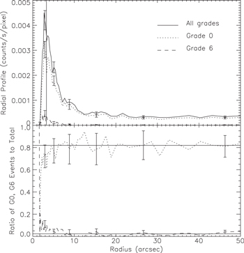
Figure 2. Radial profile for 4U 1724–308 in the 2.0 keV band for events of different grades. In the top plot, the solid line corresponds to a pile up fraction of 10%. In the bottom plot, the solid lines correspond to the grade ratio limits.
Download figure:
Standard image High-resolution imageThe data for Cyg X-2, GX 5–1, and GX 9+1 were treated in a similar way and also showed evidence of pile up at significant distances from the sources. Spectra for these four Chandra data sources were extracted from the transfer streaks, following the method detailed at the CXC website.6 The streaks for 4U 1724–307, Cyg X-2, GX 5–1, and GX 9+1 were extracted in boxes of size 800 × 6 pix, 400 × 6 pix, 700 × 6 pix, and 400 × 5 pix, respectively. These narrow extraction regions tightly followed the streaks, so that the streaks filled the boxes as completely as possible. New effective exposure times were calculated and applied to the spectra by considering the ACIS frame time, the frame transfer time, and the extraction region sizes; as an example we again consider 4U 1724–307. The time needed to move charge from one row to another is 40 μs, so the time needed to read out a chip with 1024 rows is 0.04 s, or about 1.26% of the ACIS frame time (3.24 s). However, only 800 rows were extracted for this source, or 78% of the rows on the chip. So the effective exposure time for the streak is 0.98% of the observation's livetime, or about 144 s. The streaks had 1.4 ± 1.2, 18.0 ± 4.2, 25.4 ± 5.0, and 12.3 ± 3.5 counts per frame, respectively, spread over the area of the extraction regions, so pile up in the streaks is not significant.
The XMM and Chandra spectra were fit over the energy range 0.3–8.0 keV, except for Vel X-1, which was fit over 0.5–8.0 keV. Commonly used models, such as power law (PL), blackbody (BB), bremsstrahlung (BR), disk blackbodies (DBB), broken power law (BPL), partial covering fraction absorption (PCFABS), Gaussian (GAU), thermal plasma (APEC), and Comptonization (COMP) were used. More information about these models and their parameters can be found at the XSPEC website.7 For all spectra, the IS absorption was ascertained using the photoelectric absorption model. X-rays are attenuated by atoms that are not fully ionized, usually helium and heavier elements; measuring the attentuation leads to the total column density of absorbing material along an LOS (Arnaud et al. 2011). After making assumptions about IS abundances, this is then typically expressed as the hydrogen column density, NH. In this work, the abundances of Anders & Grevesse (1989) are used. The best fits, their parameters, values of NH, and χ2 are listed in Table 4.
Table 4. Spectral Fits
| Object | Fit (plus abs) | N a
a
|
Parametersb and Fluxesc | χ2 |
|---|---|---|---|---|
| IGR J17497–2821 | PL | 4.01 ± 0.04 | Γ = 1.58 ± 0.02, FX = 7.6 × 10⁻¹⁰ | 1.12 |
| XTE J1807–294 | PL | 0.66 ± 0.01 | Γ = 1.96 ± 0.02, FX = 2.5 × 10⁻¹⁰ | 0.92 |
| 4U 1820–30 | PL + BB | 0.29 ± 0.01 | Γ = 1.78 ± 0.01, kT = 2.01 ± 0.04, FX = 1.3 × 10⁻⁸ | 1.96 |
| GX 5–1 | PL | 4.18 ± 0.06 | Γ = 1.84 ± 0.03,FX = 1.9 × 10⁻⁸ | 0.85 |
| GX 9+1 | BB | 1.24 ± 0.05 | kT = 1.21 ± 0.02, FX = 6.8 × 10⁻⁹ | 0.83 |
| GX 13+1 | BR | 2.75 ± 0.03 | kT = 3.43 ± 0.06, FX = 7.4 × 10⁻⁹ | 1.01 |
| Swift J1753.5–0127 | PL + BB | 0.24 ± 0.01 | Γ = 1.62 ± 0.02, kT = 0.24 ± 0.02, FX = 4.7 × 10⁻¹⁰ | 1.13 |
| 4U 1850–087 | BR | 0.40 ± 0.01 | kT = 2.72 ± 0.03, FX = 1.9 × 10⁻¹⁰ | 0.97 |
| IGR J18450–0435 | BB | 1.18 ± 0.08 | kT = 1.85 ± 0.05, FX = 1.9 × 10⁻¹¹ | 0.67 |
| XTE J1901+014 | DBB | 1.91 ± 0.06 | Tin = 1.97 ± 0.07 FX = 3.2 × 10⁻¹¹ | 0.81 |
| 4U 1908+005 | BR | 0.50 ± 0.01 | kT = 4.43 ± 0.11, FX = 2.6 × 10⁻¹⁰ | 0.79 |
| GRS 1915+105 | PL | 3.43 ± 0.03 | Γ = 2.59 ± 0.02, FX = 2.6 × 10⁻⁸ | 1.51 |
| 4U 1957+11 | BPL | 0.22 ± 0.01 |
 = 1.55 ± 0.01, = 1.55 ± 0.01,  = 2.74 ± 0.03, xb = 3.93 ± 0.04, FX = 1.4 × 10−9 = 2.74 ± 0.03, xb = 3.93 ± 0.04, FX = 1.4 × 10⁻⁹ |
1.28 |
| Cyg X-2 | DBB | 0.19 ± 0.01 | Tin = 1.45 ± 0.02, FX = 1.2 × 10⁻⁸ | 0.98 |
| X Per | DBB | 0.25 ± 0.01 | Tin = 3.16 ± 0.04, FX = 1.2 × 10⁻⁹ | 1.25 |
| 4U 0614+091 | PL | 0.28 ± 0.01 | Γ = 2.20 ± 0.01, FX = 9.4 × 10⁻¹⁰ | 2.68 |
| Vel X-1 | PL + 3 GAU + COMP | 0.23 ± 0.01 | Γ = 1.30 ± 0.01, LE1 = 6.41 ± 0.01, LW1 = 0.002 ± 0.02, | 1.17 |
| LE2 = 0.92 ± 0.01, LW2 = 0.04 ± 0.01, LE3 = 1.34 ± 0.01, LW3 = 0.09 ± 0.01, | ||||
| kT = 2.04 ± 0.14, τ = 27.0 ± 0.6, FX(0.5–8 keV) = 1.0 × 10⁻⁹ | ||||
| 4U 0919–54 | PL + BB | 0.28 ± 0.01 | Γ = 2.13 ± 0.03, kT = 0.51 ± 0.03, FX = 2.1 × 10⁻¹⁰ | 1.01 |
| 2S 0921–630 | PL + BB | 0.23 ± 0.01 | Γ = 1.67 ± 0.05, kT = 1.75 ± 0.03, FX = 1.0 × 10⁻¹⁰ | 1.31 |
| 4U 1119–603 | PCFABS + PL | 0.73 ± 0.12 | cfract = 0.88 ± 0.11,  = 29.11 ± 4.22, Γ = 1.32 ± 0.54, = 29.11 ± 4.22, Γ = 1.32 ± 0.54, |
1.57 |
| + 5 GAU | LE1 = 6.41 ± 0.01, LW1 = 0.04 ± 0.01, LE2 = 6.70 ± 0.02, LW2 = 0.2 ± 0.03, | |||
| LE3 = 6.99 ± 0.01, LW3 = 0.04 ± 0.03, LE4 = 3.10 ± 0.19, LW4 = 0.99 ± 0.05, | ||||
| LE5 = 1.28 ± 0.01, LW5 = 0.29 ± 0.01, FX = 2.9 × 10⁻¹⁰ | ||||
| 1A 1246–588 | PL | 0.42 ± 0.01 | Γ = 2.30 ± 0.01, FX = 1.6 × 10⁻¹⁰ | 1.32 |
| 4U 1323–62 | DBB | 2.46 ± 0.02 | Tin = 2.13 ± 0.02, FX = 2.6 × 10⁻¹⁰ | 1.17 |
| 4U 1538–52 | APEC + COMP | 1.43 ± 0.26 | kTapec = 5.36 ± 2.21,  = 12.83 ± 0.29, = 12.83 ± 0.29, |
0.82 |
| + GAU | kTcomp = 3.13 ± 0.09, τ = 44.5 ± 0.46, LE = 6.41 ± 0.01, | |||
| LW = 0.04 ± 0.02, FX = 5.0 × 10⁻¹¹ | ||||
| 4U 1608–52 | PL | 1.36 ± 0.04 | Γ = 2.36 ± 0.04, FX = 8.9 × 10⁻⁹ | 0.93 |
| 4U 1624–49 | BR | 0.85 ± 0.01 | kT = 6.05 ± 0.03,  = 7.86 ± 0.01, FX = 1.4 × 10−9 = 7.86 ± 0.01, FX = 1.4 × 10⁻⁹ |
1.96 |
| 4U 1659–487 | PL + BB | 0.62 ± 0.01 | Γ = 2.68 ± 0.02, kT = 1.87 ± 0.02, FX = 1.6 × 10⁻⁹ | 2.65 |
| SAX J1711.6–3808 | DBB | 1.95 ± 0.03 | Tin = 2.26 ± 0.05, FX = 1.0 × 10⁻⁹ | 1.00 |
| 4U 1705–32 | PL | 0.47 ± 0.01 | Γ = 1.84 ± 0.02, FX = 5.1 × 10⁻¹¹ | 0.92 |
| 4U 1746–37 | PL | 0.44 ± 0.01 | Γ = 1.50 ± 0.01, FX = 1.2 × 10⁻⁹ | 1.06 |
| 4U 1704–30 | BPL | 0.33 ± 0.01 |
 = 1.60 ± 0.01, = 1.60 ± 0.01,  = 3.36 ± 0.29, xb = 5.89 ± 0.16 = 3.36 ± 0.29, xb = 5.89 ± 0.16 |
1.31 |
| FX = 8.1 × 10⁻¹⁰ | ||||
| XTE J1720–318 | BPL | 1.78 ± 0.02 |
 = 3.68 ± 0.05, = 3.68 ± 0.05,  = 5.50 ± 0.08, xb = 2.85 ± 0.06 = 5.50 ± 0.08, xb = 2.85 ± 0.06 |
1.04 |
| FX = 1.3 × 10⁻⁸ | ||||
| 4U 1724–307 | PL | 0.66 ± 0.05 | Γ = 1.73 ± 0.06, FX = 6.0 × 10⁻¹⁰ | 0.60 |
| XTE J1710–281 | PL + BB | 0.35 ± 0.01 | Γ = 1.90 ± 0.03, kT = 22.1 ± 0.1, FX = 4.4 × 10⁻¹¹ | 0.92 |
| XTE J1751–305 | PL | 1.30 ± 0.02 | Γ = 1.61 ± 0.02, FX = 8.5 × 10⁻¹⁰ | 0.99 |
| IGRJ 17544–2619 | PL | 1.12 ± 0.08 | Γ = 0.15 ± 0.06, FX = 3.2 × 10⁻¹¹ | 1.04 |
Notes.
aNH is in units of 1022 cm−2. bTin is the temperature of the inner disk in keV, LE is the line energy in keV, LW is the line width in keV, kT is the temperature in keV, and xb is the break point. cFluxes are over the range 0.3–8 keV, unless otherwise stated, and given in units of ergs cm−2 s−1.Download table as: ASCIITypeset image
4. THE XMM-NEWTON AND CHANDRA POINT-SPREAD FUNCTIONS
The surface brightness of an object is the sum of three things: the background, the instrumental PSF, and the dust-scattered halo itself. So before fitting the halos, the PSFs of the instruments had to be found. The radial profiles of extremely bright, unreddened sources can be used to find an instrument's PSF. Her X-1, with a neutral H column density of about 2 × 1020 cm−2 within 1° of the source (Kalberla et al. 2005), is a good target for the empirical determination of the Chandra/ACIS PSF; Smith et al. (2002) showed that Her X-1 agrees with SAOsac's modeled PSF at low radial distances, but the model underpredicts the scattered light at radii >50''. Following Smith et al. (2002) and Valencic et al. (2009), we used Her X-1 (ObsID 3662) to find the PSF by processing the event file using the standard procedures as described in the CXC's Science Threads.8 The event file was divided into the same energy bins, over the same energy range, as for the absorbed sources (i.e., energy bands 0.5 keV wide), with central bin energies from 1.0 to 4.0 keV. In each energy band, radial profiles were extracted and fitted with a PL + constant,

where A is the amplitude, γ is the photon index, θ is the angle from the source,  is the normalization reference point, and C is the background.
Unreddened sight lines were also examined to determine the PSF of the XMM-Newton/EPIC-MOS instrument, beginning with the sight line toward Mkn 421 (ObsID 0136541101). The neutral H survey of Kalberla et al. (2005) shows that within 1° of the source, the column density is very low (1.9 × 1020 cm−2). The data were processed according to standard procedures,9 and the event file was divided into bands of 0.5 keV in width for energies in the range 0.75–4.25 keV, so for example, the 1.0 keV band was composed of photons with energy from 0.75 to 1.25 keV, the 1.5 keV band was composed of photons with energy from 1.25 to 1.75 keV, and so on. Spectra from the MOS cameras were extracted and fitted for MOS1, MOS2, and a joint fitting of MOS1 and MOS2. The radial profiles were also extracted and fitted in each band for those cameras seperately and jointly, with a standard PL+constant and a BPL+constant,

for  , and
, and

for  , where

where A,  , and C are as previously defined for the PL, θb is the break point, and
  and γ2 are the first and second photon indices, respectively. The BPL consistently provided better fits to the radial profiles than a standard PL. To confirm this, the radial profiles of two other bright, unreddened sources were examined: LMC X-3 (ObsID 0126500101; NH ∼ 4.3 × 1020 cm−2 Kalberla et al. 2005) and 3C 273 (ObsID 0126700501; NH ∼ 1.7 × 1020 cm−2 Kalberla et al. 2005). The data were processed in the same way as Mkn 421, and again, the radial profiles were better fit with a BPL than with a PL. A comparison of the fitting parameters and their dependence on the energy band is shown in Figure 3 for the joint MOS1+MOS2 fit, which is similar to the fits to the M1 and M2 alone. The fitting parameters are largely similar for the different sources, despite the large range in fluxes, from about 0.2 × 10⁻¹⁰ erg cm−2 s−1 (LMC X-3) to
  (Mkn 421). It should be noted that both XMM and Chandra have a quiescent background contribution at 1.5 and 1.7 keV from particles interacting with the silicon and aluminum in the detectors and their surrounding structures. Chandra also has a contribution from gold at 2.2 keV. These have been examined by the XMM and Chandra teams and typically do not show large variations in time.10
,11
While all the fits provided reasonable values of χ2, the Mkn 421 fits were consistently better than the others for all cameras. For Mkn 421, χ2ranged from 1.0 to 1.2 for the M1 and M2 fits, and 1.1 to 1.2 for the joint fits, over all 2.0–3.5 keV energy bands. This contrasts with LMC X-3's χ2 values between 1.1 and 1.3 for M1, 1.3 and 1.4 for M2, and 1.2 and 1.6 for the joint fit over the same bands. Similarly, 3C 273 produced χ2 between 1.2 and 1.6, 1.3 and 1.4, and 1.2 and 2.1 for the joint fit. Thus, the BPL fitting parameters from Mkn 421 were used as the PSF measurements in the subsequent halo fits.
(Mkn 421). It should be noted that both XMM and Chandra have a quiescent background contribution at 1.5 and 1.7 keV from particles interacting with the silicon and aluminum in the detectors and their surrounding structures. Chandra also has a contribution from gold at 2.2 keV. These have been examined by the XMM and Chandra teams and typically do not show large variations in time.10
,11
While all the fits provided reasonable values of χ2, the Mkn 421 fits were consistently better than the others for all cameras. For Mkn 421, χ2ranged from 1.0 to 1.2 for the M1 and M2 fits, and 1.1 to 1.2 for the joint fits, over all 2.0–3.5 keV energy bands. This contrasts with LMC X-3's χ2 values between 1.1 and 1.3 for M1, 1.3 and 1.4 for M2, and 1.2 and 1.6 for the joint fit over the same bands. Similarly, 3C 273 produced χ2 between 1.2 and 1.6, 1.3 and 1.4, and 1.2 and 2.1 for the joint fit. Thus, the BPL fitting parameters from Mkn 421 were used as the PSF measurements in the subsequent halo fits.
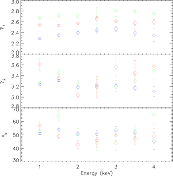
Figure 3. PSF broken power-law fit parameters in different energy bands for a joint fitting of MOS1+MOS2. The sources are LMC X-3 (green), 3C 273 (red), and Mkn 421 (blue).
Download figure:
Standard image High-resolution imageThe results from fitting the 2.5 keV band radial profiles for both Her X-1 and Mkn 421 are listed in Table 5.
Table 5. Point-spread Function Parameters in 2.5 keV Band
| Detector | Parameters |
|---|---|
| M1 | A = (2.9 ± 0.7) × 10−4, γ1 = 2.50 ± 0.12, γ2 = 3.24 ± 0.05, θb = 49 ± 5 |
| M2 | A = (4.7 ± 1.4) × 10−4, γ1 = 2.21 ± 0.15, γ2 = 3.19 ± 0.05, θb = 47 ± 8 |
| M1+M2 | A = (3.4 ± 0.3) × 10−4, γ1 = 2.41 ± 0.04, γ2 = 3.20 ± 0.03, θb = 49 ± 3 |
| ACIS | A = (3.4 ± 0.2) × 10−4, γ = 1.92 ± 0.02 |
Download table as: ASCIITypeset image
5. ANALYSIS AND RESULTS
As noted in Section 4, the measured surface brightness of a source is the sum of the background, the PSF, and the dust-scattered halo. The dust models that were considered were those of MRN, WD, and ZDA. These models assume a ratio of total to selective visual extinction RV = 3.1, which is the standard Galactic value. RV in the Galaxy ranges from 2.5 to 5.5, with denser sight lines having higher values, likely due to grain growth (Cardelli et al. 1989). In addition to modeling sight lines with RV = 3.1, WD also provided models for RV = 4.0 and 5.5.
The method of Smith et al. (2002) was followed closely. The fits were made over 67 log-spaced annuli, centered by eye on the source. The annuli were also used with the exposure maps for each energy band to find the total effective area for each band and radial distance. The radial profiles of the events data were divided by the radial profiles of the exposure maps, with the result then divided by the source flux for each energy band. This was then fitted by simultaneously fitting the contributions from the background, PSF, and the scattering expected from the dust grain models in the single-cloud and smooth distributions. An example fit is shown in Figure 4.
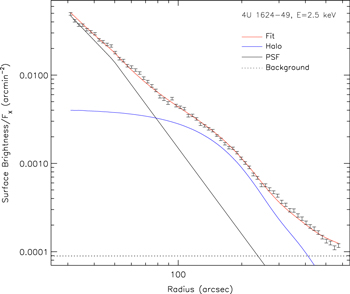
Figure 4. Example of a radial profile and its fit using MRN-type dust in a single-cloud distribution.
Download figure:
Standard image High-resolution imageThe resulting fits produced estimates of NH, and in the case of the single-cloud distributions, estimates of the relative cloud position along the LOS, x0, which ranges in value from 0 (the observer's location) to 1 (the source's location). The single-cloud distributions consistently produced better χ2 values than the smooth distributions, with differences in χ2 ranging from ∼0.001 to more than 10. Of the 35 sources in this study, 27 yielded good fits to their halos, that is, low values of χ2 and physically realistic values for NH and x0. The fitting results are listed in Tables 6–10. The remaining eight sources did not meet these requirements and examination of their halo fits showed deviations from the model beyond 3σ. These eight were then re-fit with all models in the two-cloud distribution, and all the RV = 4.0 and RV = 5.5 models of WD (from their Table 1) in both the smooth and single-cloud distributions. None of these additional fits produced better results. These sight lines are discussed further in Section 6.1.
Table 6. Resultsa to the Single Cloud Halo Fits for MRN and WD Models
| Object | MRN | WD | ||||
|---|---|---|---|---|---|---|
| NH | x0 | χ2 | NH | x0 | χ2 | |
| IGRJ 18450–0435 | 6.21 ± 1.39 | 0.43 ± 0.10 | 1.0 | 4.45 ± 0.93 | 0.35 ± 0.13 | 1.0 |
| SAX J1711.6–3808 | 7.65 ± 0.16 | 0.14 ± 0.02 | 1.6 | ⋯ | ⋯ | ⋯ |
| Swift J1753.3–0127 | 1.09 ± 0.06 | 0.49 ± 0.03 | 1.2 | 0.80 ± 0.04 | 0.40 ± 0.03 | 1.2 |
| XTE J1710–281 | 2.71 ± 0.77 | 0.91 ± 0.02 | 1.1 | 1.66 ± 0.67 | 0.91 ± 0.02 | 1.1 |
| XTE J1751–305 | 2.74 ± 0.12 | 0.29 ± 0.04 | 0.9 | 1.96 ± 0.08 | 0.15 ± 0.04 | 0.9 |
| XTE J1807–294 | 1.81 ± 0.16 | 0.62 ± 0.03 | 1.2 | 1.38 ± 0.11 | 0.55 ± 0.04 | 1.2 |
| XTE J1901+014 | 9.59 ± 0.96 | 0.43 ± 0.05 | 0.8 | 7.26 ± 0.66 | 0.36 ± 0.06 | 0.8 |
| 1A 1246–5887 | 3.71 ± 0.10 | 0.79 ± 0.01 | 1.4 | 2.47 ± 0.13 | 0.75 ± 0.01 | 1.4 |
| 2S 0921–630 | 1.26 ± 0.15 | 0.84 ± 0.02 | 1.3 | 0.96 ± 0.19 | 0.88 ± 0.01 | 1.2 |
| 4U 0614+091 | 1.34 ± 0.09 | 0.60 ± 0.03 | 1.3 | 1.00 ± 0.07 | 0.53 ± 0.03 | 1.4 |
| 4U 0919–54 | 1.17 ± 0.12 | 0.71 ± 0.03 | 1.1 | 0.82 ± 0.09 | 0.66 ± 0.04 | 1.1 |
| 4U 1323–62 | 24.4 ± 0.5 | 0.34 ± 0.01 | 2.3 | 18.0 ± 0.3 | 0.24 ± 0.01 | 2.4 |
| 4U 1608–52 | 4.80 ± 0.11 | 0.76 ± 0.01 | 1.2 | 2.17 ± 0.08 | 0.68 ± 0.01 | 1.5 |
| 4U 1624–49 | 11.0 ± 0.1 | 0.13 ± 0.01 | 3.2 | ⋯ | ⋯ | ⋯ |
| 4U 1659–487 | 1.33 ± 0.02 | 0.22 ± 0.02 | 6.7 | ⋯ | ⋯ | ⋯ |
| 4U 1704–30 | 2.14 ± 0.07 | 0.45 ± 0.02 | 2.3 | 1.43 ± 0.05 | 0.30 ± 0.03 | 2.4 |
| 4U 1705–32 | 3.88 ± 0.50 | 0.81 ± 0.03 | 1.3 | 1.16 ± 0.27 | 0.48 ± 0.10 | 1.2 |
| 4U 1724–307 | 4.83 ± 0.12 | 0.20 ± 0.02 | 1.5 | ⋯ | ⋯ | ⋯ |
| 4U 1746–37 | 1.73 ± 0.09 | 0.58 ± 0.02 | 1.6 | 1.25 ± 0.07 | 0.50 ± 0.02 | 1.7 |
| 4U 1850–087 | 0.52 ± 0.11 | 0.49 ± 0.06 | 1.4 | 0.44 ± 0.08 | 0.46 ± 0.07 | 1.4 |
| 4U 1908+005 | 3.52 ± 0.16 | 0.76 ± 0.01 | 1.2 | 1.45 ± 0.11 | 0.72 ± 0.02 | 1.2 |
| 4U 1957+11 | 1.21 ± 0.03 | 0.62 ± 0.01 | 3.9 | 1.16 ± 0.02 | 0.59 ± 0.01 | 3.7 |
| Cyg X-2 | 0.32 ± 0.01 | 0.30 ± 0.02 | 1.4 | ⋯ | ⋯ | ⋯ |
| GX 9+1 | 6.99 ± 0.05 | 0.20 ± 0.01 | 2.8 | ⋯ | ⋯ | ⋯ |
| Vel X-1 | 15.0 ± 0.1 | 0.88 ± 0.01 | 1.6 | 6.37 ± 0.77 | 0.88 ± 0.01 | 1.6 |
| IGRJ 17497–2821 | 6.49 ± 0.10 | 0.43 ± 0.01 | 1.8 | 4.83 ± 0.07 | 0.34 ± 0.01 | 1.5 |
| X Per | 0.85 ± 0.04 | 0.41 ± 0.02 | 1.3 | 0.60 ± 0.03 | 0.30 ± 0.03 | 1.3 |
Note.
aNH is in units of 1021 cm−2.Download table as: ASCIITypeset image
Table 7. Resultsa to the Single Cloud Halo Fits for ZDA BARE-AC Models
| Object | BARE-AC-B | BARE-AC-FG | BARE-AC-S | ||||||
|---|---|---|---|---|---|---|---|---|---|
| NH | x0 | χ2 | NH | x0 | χ2 | NH | x0 | χ2 | |
| IGRJ 18450–0435 | 8.32 ± 1.85 | 0.50 ± 0.09 | 1.0 | 6.45 ± 1.44 | 0.41 ± 0.11 | 1.0 | 6.59 ± 1.47 | 0.41 ± 0.11 | 1.0 |
| SAX J1711.6–3808 | 10.3 ± 0.2 | 0.23 ± 0.02 | 1.5 | 7.95 ± 0.16 | 0.10 ± 0.02 | 1.5 | 8.15 ± 0.17 | 0.10 ± 0.02 | 1.5 |
| Swift J1753.3–0127 | 1.40 ± 0.08 | 0.53 ± 0.03 | 1.2 | 1.09 ± 0.06 | 0.45 ± 0.03 | 1.2 | 1.11 ± 0.07 | 0.45 ± 0.03 | 1.2 |
| XTE J1710–281 | 2.05 ± 1.03 | 0.92 ± 0.03 | 1.1 | 1.77 ± 0.80 | 0.91 ± 0.03 | 1.1 | 1.75 ± 0.75 | 0.90 ± 0.03 | 1.1 |
| XTE J1751–305 | 3.74 ± 0.17 | 0.38 ± 0.03 | 0.9 | 2.89 ± 0.13 | 0.27 ± 0.04 | 0.9 | 2.96 ± 0.13 | 0.28 ± 0.04 | 0.9 |
| XTE J1807–294 | 2.56 ± 0.22 | 0.66 ± 0.03 | 1.2 | 1.96 ± 0.17 | 0.61 ± 0.03 | 1.2 | 2.02 ± 0.17 | 0.61 ± 0.03 | 1.2 |
| XTE J1901+014 | 13.4 ± 1.3 | 0.52 ± 0.05 | 0.8 | 10.3 ± 1.0 | 0.43 ± 0.06 | 0.8 | 10.5 ± 1.0 | 0.44 ± 0.06 | 0.8 |
| 1A 1246–5887 | 6.93 ± 0.23 | 0.81 ± 0.01 | 1.3 | 5.53 ± 0.18 | 0.78 ± 0.01 | 1.3 | 5.96 ± 0.19 | 0.78 ± 0.01 | 1.3 |
| 2S 0921–630 | 4.27 ± 0.18 | 0.81 ± 0.01 | 1.1 | 1.14 ± 0.24 | 0.89 ± 0.02 | 1.2 | 1.15 ± 0.24 | 0.88 ± 0.02 | 1.3 |
| 4U 0614+091 | 1.56 ± 0.12 | 0.62 ± 0.03 | 1.4 | 1.24 ± 0.10 | 0.56 ± 0.03 | 1.4 | 1.26 ± 0.10 | 0.56 ± 0.03 | 1.4 |
| 4U 0919–54 | 1.00 ± 0.16 | 0.71 ± 0.04 | 1.1 | 0.78 ± 0.13 | 0.66 ± 0.05 | 1.1 | 0.83 ± 0.13 | 0.67 ± 0.05 | 1.1 |
| 4U 1323–62 | 33.5 ± 0.6 | 0.43 ± 0.01 | 2.5 | 25.9 ± 0.5 | 0.33 ± 0.01 | 2.4 | 26.5 ± 0.5 | 0.33 ± 0.01 | 2.5 |
| 4U 1608–52 | 3.28 ± 0.14 | 0.75 ± 0.01 | 1.4 | 2.73 ± 0.11 | 0.71 ± 0.01 | 1.4 | 2.84 ± 0.12 | 0.71 ± 0.01 | 1.4 |
| 4U 1624–49 | 15.2 ± 0.1 | 0.22 ± 0.01 | 2.7 | 11.8 ± 0.1 | 0.09 ± 0.01 | 2.8 | 12.0 ± 0.1 | 0.10 ± 0.01 | 2.7 |
| 4U 1659–487 | 1.78 ± 0.03 | 0.31 ± 0.01 | 6.6 | 1.38 ± 0.02 | 0.20 ± 0.02 | 6.7 | 1.42 ± 0.02 | 0.21 ± 0.02 | 6.6 |
| 4U 1704–30 | 2.73 ± 0.09 | 0.48 ± 0.02 | 2.3 | 2.13 ± 0.07 | 0.40 ± 0.02 | 2.4 | 2.18 ± 0.07 | 0.41 ± 0.02 | 2.3 |
| 4U 1705–32 | 1.99 ± 0.51 | 0.58 ± 0.08 | 1.2 | 1.56 ± 0.40 | 0.51 ± 0.09 | 1.2 | 1.58 ± 0.41 | 0.51 ± 0.09 | 1.2 |
| 4U 1724–307 | 6.59 ± 0.15 | 0.29 ± 0.01 | 1.5 | 5.09 ± 0.12 | 0.17 ± 0.02 | 1.5 | 5.22 ± 0.12 | 0.18 ± 0.02 | 1.5 |
| 4U 1746–37 | 2.10 ± 0.12 | 0.61 ± 0.02 | 1.7 | 1.65 ± 0.09 | 0.54 ± 0.02 | 1.7 | 1.68 ± 0.09 | 0.54 ± 0.02 | 1.7 |
| 4U 1850–087 | 0.68 ± 0.15 | 0.56 ± 0.08 | 1.4 | 0.53 ± 0.12 | 0.48 ± 0.08 | 1.4 | 0.53 ± 0.12 | 0.48 ± 0.09 | 1.4 |
| 4U 1908+005 | 0.86 ± 0.20 | 0.76 ± 0.04 | 1.3 | 0.84 ± 0.15 | 0.73 ± 0.04 | 1.3 | 0.76 ± 0.16 | 0.73 ± 0.04 | 1.3 |
| 4U 1957+11 | 1.92 ± 0.05 | 0.68 ± 0.01 | 4.0 | 1.45 ± 0.04 | 0.62 ± 0.01 | 4.0 | 1.48 ± 0.04 | 0.63 ± 0.01 | 4.0 |
| Cyg X-2 | 0.43 ± 0.01 | 0.37 ± 0.02 | 1.4 | 0.33 ± 0.01 | 0.26 ± 0.03 | 1.4 | 0.34 ± 0.01 | 0.27 ± 0.03 | 1.4 |
| GX 9+1 | 9.54 ± 0.07 | 0.28 ± 0.01 | 1.8 | 7.35 ± 0.05 | 0.16 ± 0.01 | 2.0 | 7.55 ± 0.06 | 0.17 ± 0.01 | 1.9 |
| Vel X-1 | 7.96 ± 1.37 | 0.90 ± 0.01 | 1.7 | 6.27 ± 0.90 | 0.86 ± 0.01 | 1.7 | 6.59 ± 0.87 | 0.86 ± 0.01 | 1.7 |
| IGRJ 17497–2821 | 8.97 ± 0.13 | 0.51 ± 0.01 | 1.8 | 6.91 ± 0.10 | 0.42 ± 0.01 | 1.7 | 7.08 ± 0.11 | 0.43 ± 0.01 | 1.8 |
| X Per | 1.12 ± 0.06 | 0.47 ± 0.02 | 1.3 | 0.87 ± 0.04 | 0.38 ± 0.03 | 1.3 | 0.89 ± 0.04 | 0.38 ± 0.03 | 1.3 |
Note.
aNH is in units of 1021 cm−2.Download table as: ASCIITypeset image
Table 8. Resultsa to the Single Cloud Halo Fits for ZDA BARE-GR Models
| Object | BARE-GR-B | BARE-GR-FG | BARE-GR-S | ||||||
|---|---|---|---|---|---|---|---|---|---|
| NH | x0 | χ2 | NH | x0 | χ2 | NH | x0 | χ2 | |
| IGRJ 18450–0435 | 8.99 ± 2.02 | 0.52 ± 0.09 | 1.0 | 6.90 ± 1.55 | 0.43 ± 0.11 | 1.0 | 7.13 ± 1.60 | 0.45 ± 0.11 | 1.0 |
| SAX J1711.6–3808 | 11.4 ± 0.2 | 0.28 ± 0.02 | 1.4 | 8.71 ± 0.17 | 0.14 ± 0.02 | 1.4 | 9.00 ± 0.18 | 0.16 ± 0.02 | 1.4 |
| Swift J1753.3–0127 | 1.56 ± 0.09 | 0.57 ± 0.03 | 1.2 | 1.19 ± 0.07 | 0.48 ± 0.03 | 1.2 | 1.24 ± 0.07 | 0.50 ± 0.03 | 1.2 |
| XTE J1710–281 | 3.27 ± 1.01 | 0.92 ± 0.02 | 1.1 | 2.60 ± 0.76 | 0.90 ± 0.02 | 1.1 | 2.52 ± 0.80 | 0.91 ± 0.03 | 1.1 |
| XTE J1751–305 | 4.17 ± 0.18 | 0.43 ± 0.03 | 0.9 | 3.17 ± 0.14 | 0.32 ± 0.03 | 0.9 | 3.29 ± 0.14 | 0.34 ± 0.03 | 0.9 |
| XTE J1807–294 | 3.06 ± 0.23 | 0.71 ± 0.02 | 1.2 | 2.21 ± 0.18 | 0.64 ± 0.03 | 1.2 | 2.35 ± 0.18 | 0.66 ± 0.03 | 1.2 |
| XTE J1901+014 | 14.9 ± 1.4 | 0.56 ± 0.05 | 0.8 | 11.6 ± 1.1 | 0.46 ± 0.06 | 0.8 | 11.6 ± 1.1 | 0.49 ± 0.05 | 0.8 |
| 1A 1246–5887 | ⋯ | ⋯ | ⋯ | ⋯ | ⋯ | ⋯ | ⋯ | ⋯ | ⋯ |
| 2S 0921–630 | 2.51 ± 0.46 | 0.93 ± 0.01 | 1.3 | 1.86 ± 0.24 | 0.89 ± 0.01 | 1.2 | 1.78 ± 0.25 | 0.90 ± 0.01 | 1.2 |
| 4U 0614+091 | 1.78 ± 0.13 | 0.65 ± 0.03 | 1.4 | 1.37 ± 0.10 | 0.58 ± 0.03 | 1.4 | 1.43 ± 0.11 | 0.60 ± 0.03 | 1.4 |
| 4U 0919–54 | 1.66 ± 0.19 | 0.77 ± 0.03 | 1.1 | 0.96 ± 0.14 | 0.70 ± 0.04 | 1.1 | 1.05 ± 0.14 | 0.71 ± 0.04 | 1.1 |
| 4U 1323–62 | 36.4 ± 0.7 | 0.47 ± 0.01 | 2.9 | 27.7 ± 0.5 | 0.35 ± 0.01 | 2.8 | 28.8 ± 0.5 | 0.38 ± 0.01 | 2.8 |
| 4U 1608–52 | 4.91 ± 0.16 | 0.79 ± 0.01 | 1.3 | 3.98 ± 0.12 | 0.75 ± 0.01 | 1.3 | 4.04 ± 0.13 | 0.76 ± 0.01 | 1.3 |
| 4U 1624–49 | 16.8 ± 0.1 | 0.27 ± 0.01 | 2.3 | 12.8 ± 0.1 | 0.13 ± 0.01 | 2.4 | 13.3 ± 0.1 | 0.16 ± 0.01 | 2.4 |
| 4U 1659–487 | 2.04 ± 0.03 | 0.39 ± 0.01 | 6.1 | 1.56 ± 0.02 | 0.29 ± 0.01 | 6.3 | 1.60 ± 0.02 | 0.30 ± 0.01 | 6.2 |
| 4U 1704–30 | 3.18 ± 0.10 | 0.55 ± 0.02 | 2.2 | 2.44 ± 0.07 | 0.46 ± 0.02 | 2.2 | 2.51 ± 0.08 | 0.47 ± 0.02 | 2.2 |
| 4U 1705–32 | 2.07 ± 0.55 | 0.60 ± 0.09 | 1.2 | 1.60 ± 0.42 | 0.52 ± 0.10 | 1.2 | 1.65 ± 0.44 | 0.54 ± 0.10 | 1.2 |
| 4U 1724–307 | 7.37 ± 0.16 | 0.34 ± 0.01 | 1.5 | 5.57 ± 0.12 | 0.21 ± 0.02 | 1.5 | 5.81 ± 0.13 | 0.24 ± 0.02 | 1.5 |
| 4U 1746–37 | 2.40 ± 0.13 | 0.64 ± 0.02 | 1.6 | 1.82 ± 0.10 | 0.57 ± 0.02 | 1.6 | 1.91 ± 0.10 | 0.59 ± 0.02 | 1.6 |
| 4U 1850–087 | 0.69 ± 0.16 | 0.57 ± 0.08 | 1.4 | 0.53 ± 0.12 | 0.47 ± 0.09 | 1.4 | 0.56 ± 0.13 | 0.51 ± 0.09 | 1.4 |
| 4U 1908+005 | 0.78 ± 0.20 | 0.77 ± 0.05 | 1.3 | 0.82 ± 0.16 | 0.74 ± 0.04 | 1.2 | 0.81 ± 0.17 | 0.74 ± 0.04 | 1.3 |
| 4U 1957+11 | 2.07 ± 0.05 | 0.72 ± 0.01 | 4.3 | 1.38 ± 0.04 | 0.64 ± 0.01 | 4.3 | 1.57 ± 0.04 | 0.66 ± 0.01 | 4.3 |
| Cyg X-2 | 0.49 ± 0.01 | 0.42 ± 0.02 | 1.4 | 0.37 ± 0.01 | 0.30 ± 0.02 | 1.4 | 0.38 ± 0.01 | 0.33 ± 0.02 | 1.4 |
| GX 9+1 | 10.7 ± 0.1 | 0.33 ± 0.01 | 1.4 | 8.12 ± 0.06 | 0.20 ± 0.01 | 1.7 | 8.43 ± 0.06 | 0.23 ± 0.01 | 1.5 |
| Vel X-1 | 22.6 ± 1.1 | 0.88 ± 0.01 | 1.6 | 19.2 ± 1.0 | 0.85 ± 0.01 | 1.6 | 12.4 ± 1.0 | 0.89 ± 0.01 | 1.6 |
| IGRJ 17497–2821 | 9.86 ± 0.14 | 0.55 ± 0.01 | 2.2 | 7.45 ± 0.11 | 0.46 ± 0.01 | 2.2 | 7.77 ± 0.11 | 0.48 ± 0.01 | 2.1 |
| X Per | 1.24 ± 0.06 | 0.50 ± 0.02 | 1.3 | 0.95 ± 0.05 | 0.41 ± 0.03 | 1.3 | 0.98 ± 0.05 | 0.43 ± 0.03 | 1.3 |
Note.
aNH is in units of 1021 cm−2.Download table as: ASCIITypeset image
Table 9. Resultsa to the Single Cloud Halo Fits for ZDA COMP-AC Models
| Object | COMP-AC-B | COMP-AC-FG | COMP-AC-S | ||||||
|---|---|---|---|---|---|---|---|---|---|
| NH | x0 | χ2 | NH | x0 | χ2 | NH | x0 | χ2 | |
| IGRJ 18450–0435 | ⋯ | ⋯ | ⋯ | ⋯ | ⋯ | ⋯ | ⋯ | ⋯ | ⋯ |
| SAX J1711.6–3808 | ⋯ | ⋯ | ⋯ | ⋯ | ⋯ | ⋯ | ⋯ | ⋯ | ⋯ |
| Swift J1753.3–0127 | ⋯ | ⋯ | ⋯ | ⋯ | ⋯ | ⋯ | ⋯ | ⋯ | ⋯ |
| XTE J1710–281 | ⋯ | ⋯ | ⋯ | 2.30 ± 1.15 | 0.89 ± 0.04 | 1.1 | 1.66 ± 0.59 | 0.77 ± 0.10 | 1.1 |
| XTE J1751–305 | ⋯ | ⋯ | ⋯ | 3.57 ± 0.15 | 0.07 ± 0.04 | 0.9 | ⋯ | ⋯ | ⋯ |
| XTE J1807–294 | ⋯ | ⋯ | ⋯ | 2.60 ± 0.20 | 0.52 ± 0.04 | 1.2 | 2.81 ± 0.20 | 0.49 ± 0.04 | 1.2 |
| XTE J1901+014 | ⋯ | ⋯ | ⋯ | 13.3 ± 1.2 | 0.31 ± 0.06 | 0.8 | ⋯ | ⋯ | ⋯ |
| 1A 1246–5887 | ⋯ | ⋯ | ⋯ | ⋯ | ⋯ | ⋯ | ⋯ | ⋯ | ⋯ |
| 2S 0921–630 | 7.11 ± 0.33 | 0.76 ± 0.01 | 1.2 | 1.44 ± 0.20 | 0.79 ± 0.03 | 1.3 | 1.52 ± 0.20 | 0.78 ± 0.03 | 1.3 |
| 4U 0614+091 | 2.37 ± 0.19 | 0.28 ± 0.06 | 1.3 | 1.56 ± 0.12 | 0.45 ± 0.04 | 1.4 | 1.52 ± 0.11 | 0.39 ± 0.05 | 1.4 |
| 4U 0919–54 | 0.79 ± 0.22 | 0.33 ± 0.19 | 1.1 | 1.07 ± 0.16 | 0.59 ± 0.06 | 1.1 | 1.06 ± 0.15 | 0.56 ± 0.06 | 1.1 |
| 4U 1323–62 | ⋯ | ⋯ | ⋯ | ⋯ | ⋯ | ⋯ | ⋯ | ⋯ | ⋯ |
| 4U 1608–52 | 4.39 ± 0.22 | 0.53 ± 0.03 | 1.4 | ⋯ | ⋯ | ⋯ | ⋯ | ⋯ | ⋯ |
| 4U 1624–49 | ⋯ | ⋯ | ⋯ | ⋯ | ⋯ | ⋯ | ⋯ | ⋯ | ⋯ |
| 4U 1659–487 | ⋯ | ⋯ | ⋯ | ⋯ | ⋯ | ⋯ | ⋯ | ⋯ | ⋯ |
| 4U 1704–30 | ⋯ | ⋯ | ⋯ | ⋯ | ⋯ | ⋯ | ⋯ | ⋯ | ⋯ |
| 4U 1705–32 | ⋯ | ⋯ | ⋯ | ⋯ | ⋯ | ⋯ | ⋯ | ⋯ | ⋯ |
| 4U 1724–307 | ⋯ | ⋯ | ⋯ | ⋯ | ⋯ | ⋯ | ⋯ | ⋯ | ⋯ |
| 4U 1746–37 | 3.15 ± 0.18 | 0.25 ± 0.05 | 1.6 | 2.10 ± 0.11 | 0.43 ± 0.03 | 1.7 | 2.09 ± 0.11 | 0.37 ± 0.03 | 1.7 |
| 4U 1850–087 | ⋯ | ⋯ | ⋯ | 0.75 ± 0.35 | 0.40 ± 0.09 | 1.4 | 0.84 ± 0.14 | 0.39 ± 0.09 | 1.4 |
| 4U 1908+005 | ⋯ | ⋯ | ⋯ | 0.78 ± 0.19 | 0.67 ± 0.07 | 1.3 | 0.39 ± 0.19 | 0.64 ± 0.18 | 1.3 |
| 4U 1957+11 | 4.66 ± 0.08 | 0.58 ± 0.01 | 5.1 | ⋯ | ⋯ | ⋯ | 2.61 ± 0.05 | 0.54 ± 0.01 | 3.9 |
| Cyg X-2 | ⋯ | ⋯ | ⋯ | ⋯ | ⋯ | ⋯ | ⋯ | ⋯ | ⋯ |
| GX 9+1 | ⋯ | ⋯ | ⋯ | ⋯ | ⋯ | ⋯ | ⋯ | ⋯ | ⋯ |
| Vel X-1 | 27.6 ± 1.5 | 0.76 ± 0.01 | 1.7 | ⋯ | ⋯ | ⋯ | 7.90 ± 1.27 | 0.84 ± 0.02 | 1.6 |
| IGRJ 17497–2821 | 15.0 ± 0.2 | 0.17 ± 0.01 | 3.3 | 8.78 ± 0.13 | 0.29 ± 0.01 | 1.7 | 8.79 ± 0.12 | 0.23 ± 0.01 | 1.8 |
| X Per | ⋯ | ⋯ | ⋯ | 1.07 ± 0.05 | 0.21 ± 0.04 | 1.3 | 1.02 ± 0.05 | 0.10 ± 0.05 | 1.3 |
Note.
aNH is in units of 1021 cm−2.Download table as: ASCIITypeset image
Table 10. Resultsa to the Single Cloud Halo Fits for ZDA COMP-GR Models
| Object | COMP-GR-B | COMP-GR-FG | COMP-GR-S | ||||||
|---|---|---|---|---|---|---|---|---|---|
| NH | x0 | χ2 | NH | x0 | χ2 | NH | x0 | χ2 | |
| IGRJ 18450–0435 | 8.18 ± 1.79 | 0.43 ± 0.11 | 1.0 | 6.44 ± 1.38 | 0.33 ± 0.13 | 1.0 | 6.10 ± 1.28 | 0.27 ± 0.15 | 1.0 |
| SAX J1711.6–3808 | ⋯ | ⋯ | ⋯ | ⋯ | ⋯ | ⋯ | ⋯ | ⋯ | ⋯ |
| Swift J1753.3–0127 | ⋯ | ⋯ | ⋯ | ⋯ | ⋯ | ⋯ | ⋯ | ⋯ | ⋯ |
| XTE J1710–281 | 3.12 ± 1.16 | 0.92 ± 0.02 | 1.1 | 2.18 ± 0.95 | 0.90 ± 0.01 | 1.1 | 2.35 ± 1.04 | 0.91 ± 0.03 | 1.1 |
| XTE J1751–305 | 3.72 ± 0.16 | 0.29 ± 0.04 | 0.9 | 2.88 ± 0.12 | 0.15 ± 0.04 | 0.9 | 2.73 ± 0.12 | 0.07 ± 0.05 | 0.9 |
| XTE J1807–294 | 2.80 ± 0.21 | 0.63 ± 0.03 | 1.2 | 2.20 ± 0.17 | 0.56 ± 0.03 | 1.2 | 2.08 ± 0.16 | 0.52 ± 0.04 | 1.2 |
| XTE J1901+014 | 13.6 ± 1.2 | 0.47 ± 0.05 | 0.8 | 10.6 ± 1.0 | 0.36 ± 0.06 | 0.8 | 10.2 ± 0.9 | 0.31 ± 0.06 | 0.8 |
| 1A 1246–5887 | ⋯ | ⋯ | ⋯ | ⋯ | ⋯ | ⋯ | ⋯ | ⋯ | ⋯ |
| 2S 0921–630 | 2.16 ± 0.38 | 0.91 ± 0.01 | 1.2 | 1.51 ± 0.31 | 0.89 ± 0.01 | 1.2 | 1.74 ± 0.35 | 0.90 ± 0.01 | 1.2 |
| 4U 0614+091 | 1.74 ± 0.12 | 0.59 ± 0.03 | 1.4 | 1.40 ± 0.10 | 0.52 ± 0.03 | 1.4 | 1.36 ± 0.09 | 0.48 ± 0.04 | 1.4 |
| 4U 0919–54 | 1.92 ± 0.17 | 0.72 ± 0.01 | 1.1 | 1.13 ± 0.13 | 0.65 ± 0.04 | 1.1 | 0.94 ± 0.12 | 0.60 ± 0.05 | 1.1 |
| 4U 1323–62 | 33.4 ± 0.6 | 0.35 ± 0.01 | 2.6 | 26.2 ± 0.5 | 0.24 ± 0.01 | 2.5 | 25.0 ± 0.5 | 0.17 ± 0.01 | 2.6 |
| 4U 1608–52 | 4.74 ± 0.15 | 0.74 ± 0.01 | 1.4 | 3.27 ± 0.11 | 0.68 ± 0.01 | 1.4 | ⋯ | ⋯ | ⋯ |
| 4U 1624–49 | ⋯ | ⋯ | ⋯ | ⋯ | ⋯ | ⋯ | ⋯ | ⋯ | ⋯ |
| 4U 1659–487 | ⋯ | ⋯ | ⋯ | ⋯ | ⋯ | ⋯ | ⋯ | ⋯ | ⋯ |
| 4U 1704–30 | ⋯ | ⋯ | ⋯ | ⋯ | ⋯ | ⋯ | ⋯ | ⋯ | ⋯ |
| 4U 1705–32 | ⋯ | ⋯ | ⋯ | ⋯ | ⋯ | ⋯ | ⋯ | ⋯ | ⋯ |
| 4U 1724–307 | 6.70 ± 0.14 | 0.18 ± 0.02 | 1.4 | ⋯ | ⋯ | ⋯ | ⋯ | ⋯ | ⋯ |
| 4U 1746–37 | 2.32 ± 0.12 | 0.58 ± 0.02 | 1.6 | 1.79 ± 0.09 | 0.49 ± 0.02 | 1.7 | 1.73 ± 0.09 | 0.45 ± 0.01 | 1.7 |
| 4U 1850–087 | 0.75 ± 0.15 | 0.53 ± 0.08 | 1.4 | 0.63 ± 0.12 | 0.46 ± 0.08 | 1.4 | 0.60 ± 0.11 | 0.42 ± 0.09 | 1.4 |
| 4U 1908+005 | 2.75 ± 0.21 | 0.77 ± 0.02 | 1.2 | 1.59 ± 0.16 | 0.71 ± 0.03 | 1.2 | 1.42 ± 0.15 | 0.69 ± 0.03 | 1.2 |
| 4U 1957+11 | 2.24 ± 0.05 | 0.66 ± 0.01 | 4.0 | 1.71 ± 0.04 | 0.59 ± 0.01 | 3.8 | 1.76 ± 0.03 | 0.56 ± 0.01 | 3.8 |
| Cyg X-2 | 0.44 ± 0.01 | 0.27 ± 0.03 | 1.4 | ⋯ | ⋯ | ⋯ | ⋯ | ⋯ | ⋯ |
| GX 9+1 | 9.67 ± 0.07 | 0.17 ± 0.01 | 1.3 | ⋯ | ⋯ | ⋯ | ⋯ | ⋯ | ⋯ |
| Vel X-1 | 6.71 ± 1.02 | 0.87 ± 0.02 | 1.6 | 11.0 ± 1.4 | 0.89 ± 0.01 | 1.6 | 9.88 ± 1.30 | 0.87 ± 0.01 | 1.6 |
| IGRJ 17497–2821 | 9.03 ± 0.13 | 0.45 ± 0.01 | 1.8 | 7.04 ± 0.10 | 0.34 ± 0.01 | 1.6 | 6.75 ± 0.10 | 0.28 ± 0.01 | 1.6 |
| X Per | 1.11 ± 0.05 | 0.39 ± 0.03 | 1.2 | 0.87 ± 0.04 | 0.28 ± 0.04 | 1.3 | 0.83 ± 0.04 | 0.21 ± 0.04 | 1.3 |
Note.
aNH is in units of 1021 cm−2.Download table as: ASCIITypeset image
Correlations between the hydrogen column density (from the spectral fits), optical extinction AV, and X-ray scattering optical depth τsca (from the halo fits) were examined. It is expected that these quantities should be linked with each other; AV and τsca rely on essentially the same grains (Predehl 1997), and as NH and AV are known to scale with each other, NH and τsca should as well. Correlations between these quantities are discussed in Sections 5.2–5.4 The sample sizes tended to be relatively small (≤27), so the Cash statistic was used to find the best fits.
5.1. Determining the Optical Extinction
For each source, the literature was scoured for measurements of AV or reddening E(B–V), which has often been used to estimate AV by the relation AV =  , where
  3.1 for the typical Galactic sight line. For sources where E(B–V) was given, this was cast as AV by assuming RV = 3.1. In cases where no uncertainties were given, the average of the quoted uncertainties, 13%, was assumed.
There were 20 objects in the survey with known AV. In order to increase the number in the sample, the HEASARC archive was searched for absorbed XRBs in globular clusters and stars with known AV. These were bright enough to have a spectrum that could be fit well, but not bright enough to have a detectable halo. Three sources were found (EXO 1745–248, HD 245770, and NGC 6440). The parameters of their spectral fits are listed in Table 11. Values of AV for all sources, with and without halos, are discussed in this section. The extinction values used in this work are summarized in Table 12. For ease of comparison, the hydrogen column densities obtained from the spectral fits (from Tables 4 and 11) are reprinted here.
Table 11. Spectrum Fit Parameters for Absorbed Objects without Detectable Halos
| Object | Fit (plus abs) |
 a
a
|
Parametersb | χ2 |
|---|---|---|---|---|
| EXO 1745–248 | DBB | 1.72 ± 0.04 | Tin = 2.76 ± 0.09 | 0.77 |
| HD 245770 | PL | 0.32 ± 0.03 | Γ = 0.51 ± 0.04 | 0.76 |
| NGC 6440 | PL | 0.65 ± 0.02 | Γ = 1.34 ± 0.03 | 0.91 |
Notes.
aNH is in units of 1022 cm−2, Tin is the temperature of the inner disk in keV. bTin is the temperature of the inner disk in keV.Download table as: ASCIITypeset image
Table 12. Sources with Measured AV
| Object | AV | NH | Comment |
|---|---|---|---|
| (mag) | (×1021 cm−2) | ||
| 4U 1820–30 | 0.87 ± 0.13 | 2.9 ± 0.1 | In NGC 6624 |
| Swift J1753.5–0127 | 1.05 ± 0.12 | 2.5 ± 0.1 | ⋯ |
| 4U 1850–087 | 1.40 ± 0.14 | 4.0 ± 0.1 | In NGC 6712 |
| IGR J18450–0435 | 7.6 ± 1.0 | 11.8 ± 0.8 | ⋯ |
| 4U 1908+005 | 1.55 ± 0.31 | 5.0 ± 0.1 | ⋯ |
| 4U 1957+11 | 1.25 ± 0.25 | 2.2 ± 0.1 | ⋯ |
| X Per | 1.21 ± 0.16 | 2.5 ± 0.1 | ⋯ |
| 4U 0614+091 | 2.73 ± 0.31 | 2.8 ± 0.1 | ⋯ |
| 4U 0919–54 | 2.17 ± 0.47 | 2.8 ± 0.1 | ⋯ |
| 2S 0921–630 | 1.02 ± 0.03 | 2.3 ± 0.1 | ⋯ |
| 4U 1119–603 | 4.30 ± 0.56 | 7.3 ± 1.2 | ⋯ |
| 4U 1538–52 | 6.80 ± 0.90 | 14.3 ± 2.6 | ⋯ |
| 4U 1608–52 | 7 ± 1 | 13.6 ± 0.4 | ⋯ |
| 4U 1659–487 | 3.7 ± 0.3 | 6.2 ± 0.1 | ⋯ |
| 4U 1746–37 | 1.46 ± 0.22 | 4.4 ± 0.1 | In NGC 6441 |
| 4U 1724–307 | 5.80 ± 0.59 | 6.6 ± 0.5 | In Terzan 2 |
| Cyg X-2 | 0.68 ± 0.16 | 1.9 ± 0.1 | ⋯ |
| XTE J1720–318 | 7 ± 1 | 17.8 ± 0.2 | ⋯ |
| IGR J17544–2619 | 6.26 ± 0.40 | 11.2 ± 0.8 | ⋯ |
| NGC 6440 | 3.32 ± 0.34 | 6.5 ± 0.2 | ⋯ |
| EXO 1745–248 | 7.04 ± 0.95 | 17.2 ± 0.4 | In Terzan 5 |
| HD 245770 | 2.29 ± 0.34 | 3.2 ± 0.3 | ⋯ |
| Vel X-1 | 2.2 ± 0.3 | 2.3 ± 0.1 | ⋯ |
Download table as: ASCIITypeset image
4U 1820–30. This LMXRB is in the globular cluster NGC 6624. A catalog of globular clusters (Harris 1996, 2010 edition) lists E(B–V) = 0.28 ± 0.03. Valenti et al.'s (2004) study of the cluster's color–magnitude diagram (CMD) and distance modulus yielded a slightly higher value, 0.34, although if the uncertainty is about 13%, these values are essentially the same. Nonetheless, Valenti et al. (2004) relied on Harris's value in their study and we do the same, leading to AV = 0.87 ± 0.13.
Swift J1753.5–0127. This soft X-ray transient was found in hard X-rays in 2005 with the Swift BAT instrument, and ground-based follow-up quickly detected the optical counterpart (Halpern 2005). It was the subject of an extensive multiwavelength campaign by Cadolle Bel et al. (2007), who obtained optical spectra and measured the width of the IS Na i doublet. This led to an estimate of the reddening, E(B–V) = 0.34 ± 0.04, or AV = 1.05 ± 0.12.
4U 1850–087. This LMXRB is in the globular cluster NGC 6712. Harris's catalog (1996, 2010 edition) listed E(B–V) = 0.45 ± 0.05, which is higher than that found by studies of the cluster's CMD by Ortolani et al. (2000; E(B–V) = 0.33) and Zinn (1980; E(B–V) = 0.39) but similar to that found by Webbink (1985; E(B–V) = 0.48) and Zinn (1985; E(B–V) = 0.48). Here we adopted Harris's value, and AV = 1.40 ± 0.14.
IGR J18450–0435. This HMXRB was discovered by ASCA and follow-up optical and IR photometry and spectra were obtained (Coe et al. 1996). These revealed that the companion is O9.5 I, and based on its colors, the authors estimate E(B–V) = 2.45, although they also note that there is large uncertainty in the extinction law for this sight line. If RV = 3.1, then AV = 7.6.
4U 1908+005. Identifying the optical counterpart in this LMXRB was a challenge. Thorstensen et al. (1978) obtained photographic photometry and spectroscopy of what was thought to be the companion. They determined that it had a spectral type between G7 and K3, with indeterminate luminosity type; given its colors and assuming it was K0 V, they estimated E(B–V) ∼ 0.37. Later studies confirmed the spectral type to be early K (Shahbaz et al. 1997), but Callanan et al. (1999) was able to resolve the system in quiesence with K-band Keck photometry and found that it was a different star than had been examined by Thorstensen et al. (1978) or Shahbaz et al. (1997). Subsequent spectroscopy by Chevalier et al. (1999) found that the companion is likely to be K7 V with E(B–V) = 0.5 ± 0.1, or AV = 1.55 ± 0.31.
4U 1957+11. Margon et al. (1978) identified the optical counterpart to this LMXRB and obtained spectra and photometry for both it and several nearby stars. From these field stars, Margon et al. estimated that AV = 1.0–1.5. We therefore take AV = 1.25 ± 0.25. As will be seen in Section 5.4, this source has an X-ray scattering optical depth (τsca) that is higher than expected for its optical extinction.
X Per. This HMXRB was studied in great detail by Telting et al. (1998). Using UV, optical, and IR data taken from the disk-free and near-disk-free states, they modeled the system and found that the companion was likely a O9.5-B0V star, similar to spectral types found by others (Hiltner 1956; Lesh 1968), and found that E(B–V) = 0.39, or AV = 1.21.
4U 0614+091. Davidsen et al. (1974) obtained photographic photometry and spectrophotometry on this LMXRB system, and argued that the reddening from nearby stars suggested E(B–V) ∼ 0.3. This was supported by work by Machin et al. (1990), who found an upper limit on the equivalent width of the DIB at 4430 Å, which led to  0.3 ± 0.2. However, the most recent study on the ISM on this sight line that included spectroscopy on the IS Na i lines provided a lower limit of
  0.4, and the strength of the DIB at 5780 Å led to E(B–V) = 0.88 ± 0.1 (Nelemans et al. 2004). We have adopted the most recent value for this work, and so AV = 2.73 ± 0.31.
4U 0919–54. Chevalier & Ilovaisky (1987) obtained optical photometry on this LMXRB system and assumed the intrinsic colors of van Paradijs (1983) to find E(B–V) = 0.3 ± 0.1, which compared favorably with an estimate of the region's extinction, AV = 1.0 (Neckel & Klare 1980). However, Nelemans et al. (2004) measured the equivalent widths of the IS Na D lines and the DIB at 5780 Å and found  0.4 and E(B–V) = 0.70 ± 0.15, respectively. For this work, we use AV = 2.17 ± 0.47.
2S 0921–630. Shahbaz et al. (1999) obtained high resolution spectra of this LMXRB system and determined that the companion is a K0 III. In a subsequent study by Shahbaz & Watson (2007) of the star's equatorial rotational velocity, the authors noted that the IS Na i doublet was clearly detected, and used it to estimate E(B–V) = 0.33 ± 0.01 for this LOS, or AV = 1.02 ± 0.03.
4U 1119–603 = Cen X-3 = V779 Cen. Krzeminski (1974) identified the optical companion in this system as a reddened O9-O9.5 V or B0 I-III based on the observed color indices. Later work by Hutchings et al. (1979) relied on spectra to suggest the companion's spectral type to be O6-O9 I. Hutchings et al. (1979) also noted the presence of DIBs at 4430, 5780, and 6254 Å, but did not use them to estimate the reddening; rather, with the star's color index and brightness, they estimate AV = 4.2. More recent work by Ash et al. (1999) concluded that the companion was likely an O6-O7 II-III, and van der Meer et al. (2007) give E(B–V) ∼ 1.4, which leads to AV = 4.3.
4U 1538–52. Cowley et al. (1977) examined Schmidt plates to find candidate optical counterparts and suggested that the counterpart was likely to be a reddened OB star. Follow-up studies by Crampton et al. (1978) and Parkes et al. (1978) confirmed that the counterpart likely had spectral type ∼B0 I, and was reddened. From the spectral type and color, Crampton et al. (1978) estimated E(B–V) = 2.4 ± 0.15, which is similar to what Parkes et al. (1978) found using the equivalent width of the DIB at 6283 Å, E(B–V) = 2.1. A study by Ilovaisky et al. (1979) also found E(B–V) = 2.16 from the counterpart's spectral type and colors. A subsequent study of the system's optical photometry by Pakull et al. (1983) suggested E(B–V) = 2.22. For this work, we adopt E(B–V) ∼ 2.2, or AV = 6.8.
4U 1608–52. Grindlay & Liller (1978) obtained I-band photometry and identified the optical counterpart. They noted that the source was not visible in photographic plates taken by other workers, which placed a lower limit on the system's  color. They then assumed that the source was similar in absolute luminosity and intrinsic colors to other X-ray transients, and set a lower limit of
  . Later, Wachter et al. (2002) obtained VRI photometry and found that the counterpart's spectral energy distribution made it most likely a late F or early G main-sequence star; this, combined with a distance estimate based from Nakamura et al. (1989) on type I X-ray bursts with photospheric radius expansion, led to an extinction estimate of 6
  8. Thus, for this work we let AV = 7 ± 1.
4U 1659–487. Grindlay (1979) found the optical counterpart in this LMXRB system and used the equivalent widths of the IS Na D lines and several DIBs seen toward nearby stars to estimate E(B–V) ∼ 1.25. Later work by Cowley et al. (1987) found a similar value, E(B–V) ∼ 1.3, by measuring the strength of the DIB at 4430 Å along the 4U 1659–487 LOS. Zdziarski et al. (1998) used a weighted mean based on these earlier studies, E(B–V) ∼ 1.2 ± 0.1, or AV = 3.7 ± 0.3. This is the value used in the current work.
4U 1746–37. This LMXRB is located in the globular cluster NGC 6441. The cluster is at low Galactic latitude and near the Galactic Center. Harris (1996, 2010 edition) gives E(B–V) = 0.47 for the cluster, and Bonatto et al. (2013) showed that it exhibits differential reddening, with E(B–V) ranging from  over the 200'' × 200'' FOV of the HST/WFC, due to the Galactic foreground ISM. For this study, we use E(B–V) = 0.47 ± 0.07, or AV = 1.46 ± 0.22.
4U 1724–307. This LMXRB is located in the globular cluster Terzan 2. Christian & Friel (1992) relied on the metallicity measurement of Armandroff & Zinn (1988) and IR photometery to find the distance modulus and reddening toward this cluster, E(B–V) = 1.25 ± 0.15. However, later work by Ortolani et al. (1997) and Valenti et al. (2009) found notably higher values, E(B–V) = 1.54 and 1.87, respectively. Harris (1996, 2010 edition) lists E(B–V) = 1.87 ± 0.19 (AV = 5.80 ± 0.59), and we use this value.
Cyg X-2. The optical counterpart in this LMXRB was suggested by Cowley et al. (1979) to be an F2 III-IV; later work by Casares et al. (1998) found that it was best described as A9 III. Goranskij & Lyutyj (1988) relied on spectra and photometry to estimate E(B–V) = 0.22 ± 0.05. This is notably lower than the reddening given by McClintock et al. (1984), who estimated E(B–V) = 0.40 ± 0.07 by essentially "ironing out" the 2175 Å bump, which was in agreement with Chiappetti et al. (1981) who also found 0.4  0.5 via the same method. However, these values are much higher than the rest of the stars within ∼2
 5 of Cyg X-2 (Cathey & Hayes 1968). To investigate further, the dust maps of Schlafly & Finkbeiner (2011) were consulted, which gave E(B–V) = 0.25, which is in agreement with that found by Goranskij & Lyutyj (1988). In this work, we take E(B–V) = 0.22 ± 0.05 (AV = 0.68 ± 0.16).
XTE J1720–318. The near-infrared (NIR) counterpart to this LMXRB was found by Nagata et al. (2003), who used the dust maps of Schlegel et al. (1998) and Dutra et al. (2003) to estimate  6–7. Chaty & Bessolaz (2006) confirmed Nagata's counterpart in the optical regime, and used optical and NIR photometry to analyze the CMD and model the spectral energy distribution. They found that the companion is most likely a main-sequence star, ranging in spectral type from late B to early G, with AV ranging from 6 to 8 mag. We therefore take AV = 7 ± 1.
IGR J17544–2619. Rodriguez (2003) announced that a likely counterpart had been detected by 2MASS, and later work by Pellizza et al. (2006) confirmed it, by obtaining the optical and NIR photometry and optical spectra of the source. The spectroscopy indicated that it is likely an O9 I. Further, several DIBs were present, and the equivalent width of the one at 5780 Å indicated E(B–V) = 1.97 ± 0.15; this is in agreement with the reddening they found with the counterpart's spectral type and color, 2.07 ± 0.11. The authors take the reddening to the system to be the average, E(B–V) = 2.02 ± 0.13, or AV = 6.26 ± 0.40.
NGC 6440. A bright LMXRB is located in this globular cluster, which is at low Galactic latitude and near the Galactic Center. The cluster has high foreground reddening, with E(B–V) = 1–1.1 (Zinn 1980; Bica & Pastoriza 1983; Ortolani et al. 1994). Harris (1996, 2010 edition) lists E(B–V) = 1.07 ± 0.11, or AV = 3.32 ± 0.34.
EXO 1745–248. This LMXRB is located in the globular cluster Terzan 5, which is known to have differential foreground reddening (Ortolani et al. 1996). Armandroff & Zinn (1988) used the DIB at 8621 Å to estimate E(B–V) = 1.65, but studies with optical or NIR photometry indicate much higher average reddenings: from 2.16 (Cohn et al. 2002) to 2.49 (Ortolani et al. 1996). Barbuy et al. (1998) and Valenti et al. (2007) estimated the reddening to be about 2.38–2.39, whereas according to Harris (1996, 2010 edition), E(B–V) = 2.28. However, Massari et al. (2012) used Hubble Space Telescope (HST) photometry to produce a high resolution extinction map of the cluster and found the reddening to be even more severe: 2.15  2.82; further, they estimate that RV = 2.83, leading to 6.09
  7.98. We therefore let AV = 7.04 ± 0.95.
HD 245770. Wade & Oke (1977) obtained optical spectra of the system and examined the counterpart as well as the reddening along the sight line. They found that the companion was likely a B0 III, and estimated E(B–V) = 0.8, based on the strengths of DIBs at 4430 and 5790 Å and the Na i D lines. This is in agreement with that found by Giangrande et al. (1980; E(B–V) = 0.83 ± 0.08), also obtained via the 4430 Å DIB, and similar to what was found in Steele et al.'s (1998) examination of this sight line, where the strengths of the Na i D2 line and the DIBs at 5780, 5797, 6269, and 6613 Å led to an average E(B–V) ∼ 0.7 ± 0.2. In Lyuty & Zaitseva's (2000) comprehensive study of the system's photometry over the span of 100 years, the authors concluded that in the system's quiescent phase E(B–V) = 0.74, which compares well with the values found by the others. For this work, we take the average, with E(B–V) = 0.74 ± 0.11, or AV = 2.29 ± 0.34.
Vel X-1 = HD 77581 = 4U 0900–40. The optical counterpart in this system was identified by Hiltner et al. (1972) as a star with spectral type B0.5 Ib. Optical photometry by van Genderen (1981) suggested  0.77, which is consistent with E(B–V) = 0.73, as found by Zuiderwijk et al. 1977 photometry. Snow et al.'s (1977) compilation of diffuse DIB measurements lists two values for the depth of the feature at 4430 Å; taking the average of these measurements and using their relation between band strength and reddening, a lower value was found: E(B–V) = 0.64. Here we have adopted E(B–V) = 0.7, or AV = 2.2. As will be seen in Section 5.4, this source has an X-ray scattering optical depth (τsca) that is higher than expected for its optical extinction.
5.2. Optical Extinction and NH
First, the relation between AV and NH from the X-ray spectral fits was considered. Figure 5 shows AV plotted against NH found by fitting the X-ray spectrum. The best-fit line is given by AV = (0.48 ± 0.06) (1021 cm−2). Many others have examined the ratio of optical extinction to NH. For comparison, their results are summarized in Table 13, as well as discussed later. Prior to the launch of ROSAT in 1990, X-ray data for these studies came from detectors on sounding rockets or the Uhuru X-ray satellite. Reina & Tarenghi (1973) used the NH of five objects reported in the literature to find AV = 0.54 × NH (1021 cm−2). Gorenstein (1975) used a sample of seven objects with NH in the literature and found AV = (0.45 ± 0.03) × NH (1021 cm−2).

Figure 5. Relation between the optical extinction and hydrogen column density from the spectral fits. The correlation between AV and NH found in this work is shown, as is that from others for comparison. Both Güver & Özel (2009) and Gorenstein (1975) found the same slope.
Download figure:
Standard image High-resolution imageTable 13. Comparison of Values of AV/NH From This Work and Other Sources
| Source | AV/NH (×1021 cm−2) |
|---|---|
| Reina & Tarenghi (1973) | 0.54 |
| Gorenstein (1975) | 0.45 ± 0.03 |
| Bohlin et al. (1978) | 0.53 ± 0.03 |
| Predehl & Schmitt (1995) | 0.56 ± 0.01 |
| Güver & Özel (2009) | 0.45 ± 0.02 |
| This work | 0.48 ± 0.06 |
Download table as: ASCIITypeset image
Twenty years later, Predehl & Schmitt (1995) examined ROSAT data and fitted the spectra of 29 objects with absorbed thermal BR, BB, and PL models. For some sources, the BR models provided better fits, while for others, the BB models were better; for all, however, the PL provided fits that were consistent with the better of the two other models. This was probably due to ROSAT's narrow bandpass (0.1–2.4 keV). The authors used the values of NH that were yielded by the PL fits, and found AV = (0.56 ± 0.01) × NH (1021 cm−2).
More recently, Güver & Özel (2009) examined the spectra of 22 supernova (SN) remnants with Chandra, Suzaku, and XMM-Newton. The spectra were fit from 0.2 to 8 keV, with typical successful fits being provided by absorbed thermal plasma, BB, BR, or PL models. Values of E(B–V) were found in the literature, where they had been determined by measuring the Balmer decrement, S ii or Fe[ ii] line ratios; AV was then found by assuming the standard Galactic reddening law. For four of their objects, these optical data did not exist, so AV was estimated by finding the extinction for nearby stars in the field with known distances. This led the authors to find AV = (0.45 ± 0.02) (1021 cm−2).
It is worth noting that the results found here, and those found in the earlier works mentioned previously, are also in reasonable agreement with those found in other wavelength regimes; Bohlin et al. (1978) used Copernicus data to examine Lyα absorption along 100 lines of sight, and found AV = (0.53 ± 0.03)  (1021 cm−2).
5.3. Scattering Optical Depth and NH From Spectral Fits
The X-ray scattering optical depth τsca was found for all sight lines and models that produced good fits. As NH was large for many of the sight lines, multiple scattering (i.e., a single photon being scattered more than once) was a concern. Multiple scattering broadens the halo, and Mathis & Lee (1991) showed that at  1.3, multiply scattered photons dominate over singly scattered, and for models like MRN and Draine & Lee (1984), the scattering cross section
  = 9.03
 ![$\times {10}^{-23}{[E(\mathrm{keV})]}^{-2}$](https://content.cld.iop.org/journals/0004-637X/809/1/66/revision1/apj516930ieqn54.gif) H−1. Thus, at an energy of 1 keV, multiple scattering will overtake single scattering in importance when NH = 1.4 × 1022 cm−2, which is comparable to the IS NH along many of these sight lines. In contrast, at an energy of 2.5 keV, single scattering still dominates over multiple scattering up to NH = 9 × 1022 cm−2. This is about twice as large as the largest value of IS NH for objects in the sample, so multiple scattering should not affect the results at that energy. The values of τsca(2.5 keV) were normalized to τsca(1.0 keV) for ease of comparison with results from previous workers by noting that τsca(1.0 keV) = τsca/[E (keV)]2 (Predehl & Schmitt 1995) assuming the RG approximation.
H−1. Thus, at an energy of 1 keV, multiple scattering will overtake single scattering in importance when NH = 1.4 × 1022 cm−2, which is comparable to the IS NH along many of these sight lines. In contrast, at an energy of 2.5 keV, single scattering still dominates over multiple scattering up to NH = 9 × 1022 cm−2. This is about twice as large as the largest value of IS NH for objects in the sample, so multiple scattering should not affect the results at that energy. The values of τsca(2.5 keV) were normalized to τsca(1.0 keV) for ease of comparison with results from previous workers by noting that τsca(1.0 keV) = τsca/[E (keV)]2 (Predehl & Schmitt 1995) assuming the RG approximation.
The results are shown in Figure 6 for a representative selection of models (MRN, WD, ZBAF, ZBGF). The number of sources that a model could fit, the best fit τsca(1.0 keV)/NH with 1σ uncertainties, and the Pearson correlation coefficients r are listed in Table 14. Three things are immediately noticeable: First, the number of sources that a model could fit varied greatly. The ZDA COMP-AC models, in particular, had difficulty fitting the halos successfully. Second, values of τsca(1.0 keV)/NH from the more successful models tended to be similar, ranging from about 0.02 to 0.03. For comparison, Predehl & Schmitt (1995) found τsca(1.0 keV)/NH = 0.05. Part of this discrepancy may be due to the fact that Predehl & Schmitt (1995) fit all their spectra with the absorbed PL model, because the narrow ROSAT bandpass allowed that model to consistently provide the best fits for their sources. It is also likely due to our choice of halo energy bandpass, as Smith & Dwek (1998) showed that RG overestimates halo intensities at low energies ( 2 keV) compared to the Mie solution. Third, values of τsca(1.0 keV)/NH showed appreciable variability among sources for a single dust model. This may be due circumstellar material around the source, and is discussed further in Section 5.4. The intent of these fits and tables is not to suggest there are significant differences between the models that can be inferred from these data, but rather to show the range of possible values and show the agreement between the data and a simple linear model.
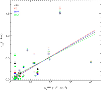
Figure 6. Comparison of the X-ray scattering optical depth at 1.0 keV and hydrogen column density from the spectral fits for a representative selection of models. The solid lines indicate the best fits. Open and filled circles correspond to objects with unknown and known AV, respectively.
Download figure:
Standard image High-resolution imageTable 14. Values of τsca(1.0 keV)/NH for Each Model
| Model | No. Sources | τsca(1.0 keV)/NH | Cstat/DOF | r |
|---|---|---|---|---|
| MRN | 27 | 0.025 ± 0.016 | 3.3/25 | 0.60 |
| WD | 21 | 0.027 ± 0.015 | 2.1/19 | 0.65 |
| ZBAB | 27 | 0.026 ± 0.013 | 3.1/25 | 0.62 |
| ZBAF | 27 | 0.026 ± 0.011 | 3.2/25 | 0.62 |
| ZBAS | 27 | 0.026 ± 0.013 | 3.2/25 | 0.62 |
| ZBGB | 26 | 0.025 ± 0.016 | 4.0/24 | 0.60 |
| ZBGF | 26 | 0.023 ± 0.016 | 4.5/24 | 0.57 |
| ZBGS | 26 | 0.027 ± 0.014 | 3.3/24 | 0.62 |
| ZCAB | 8 | 0.007 ± 0.015 | 0.6/6 | 0.65 |
| ZCAF | 12 | 0.016 ± 0.015 | 0.5/10 | 0.78 |
| ZCAS | 12 | 0.010 ± 0.024 | 0.2/10 | 0.94 |
| ZCGB | 20 | 0.026 ± 0.012 | 2.3/18 | 0.63 |
| ZCGF | 17 | 0.027 ± 0.013 | 2.1/15 | 0.64 |
| ZCGS | 16 | 0.029 ± 0.019 | 2.0/14 | 0.65 |
Download table as: ASCIITypeset image
5.4. Scattering Optical Depth and AV
The ratio of τsca/AV for each model was also examined. Of the 27 sources with halos that were well fit, 15 had values of AV from the literature. The MRN and ZDA BARE- models had the most, whereas the ZDA COMP-AC models had the least (<10); with such few data points, the ZDA COMP-AC models were not considered further. In cases where no uncertainties were given with reddening estimates, the average of the quoted uncertainties, 13%, was again assumed. The values of τsca(1.0 keV) and AV are plotted in Figure 7 for a representative selection of models (MRN, WD, ZBAS, and ZBGS). Again, these fits are shown simply to demonstrate the range of possible values obtained from different dust models.
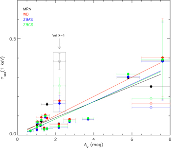
Figure 7. Comparison of the X-ray scattering optical depth at 1.0 keV and optical extinction AV from the literature for a representative selection of models. The solid lines indicate the best fits. Open circles indicate sources that were not used in finding the best fits. Vel X-1, which is discussed in Section 6.3, is indicated.
Download figure:
Standard image High-resolution imageAll models had sources with notably high or low τsca for its AV, with Vel X-1 being one of the most common. This LOS is discussed further in Section 6.3. The values of τsca(1.0 keV) found without such sources, their 1σ uncertainties, and the correlation coefficients for all models are listed in Table 15. The values of τsca(1.0 keV)/AV ranged from 0.04 to 0.05. For comparison, Predehl & Schmitt (1995) found τsca(1.0 keV)/AV ∼ 0.06.
Table 15. Values of τsca(1.0 keV)/AV
| Model | No. Sources | τsca(1.0 keV)/AV | Cstat/DOF | r |
|---|---|---|---|---|
| MRN | 14 | 0.041 ± 0.032 | 0.2/12 | 0.91 |
| WD | 11 | 0.050 ± 0.047 | 0.2/9 | 0.93 |
| ZBAB | 14 | 0.041 ± 0.030 | 0.3/12 | 0.92 |
| ZBAF | 14 | 0.045 ± 0.030 | 0.2/12 | 0.93 |
| ZBAS | 14 | 0.045 ± 0.030 | 0.2/12 | 0.92 |
| ZBGB | 13 | 0.045 ± 0.032 | 0.2/11 | 0.94 |
| ZBGF | 13 | 0.046 ± 0.033 | 1.2/11 | 0.95 |
| ZBGS | 13 | 0.044 ± 0.037 | 0.2/11 | 0.94 |
| ZCGB | 12 | 0.053 ± 0.042 | 0.1/10 | 0.96 |
| ZCGF | 10 | 0.050 ± 0.023 | 0.1/8 | 0.94 |
| ZCGS | 10 | 0.050 ± 0.023 | 0.2/8 | 0.93 |
Download table as: ASCIITypeset image
It is interesting to compare the values of the correlation coefficients for each model's τsca/NH (Table 14) and of τsca/AV (Table 15). Values of τsca/AV showed far less variability among sources for a single dust model than τsca/NH. This may be because the values for AV were obtained independently of the X-ray source, via examination of the optical counterpart, IS absorption lines, or the cluster's characteristics (if the system was in a globular cluster). In contrast, NH was obtained by fitting the X-ray spectrum and therefore includes contributions from both the ISM and any circumstellar material that may be at the X-ray source. This suggests that the AV–NH correlation seen in Figure 5 may be used to gauge how much local absorption a system has, because a value of AV/NH that is much lower than expected may indicate the presence of excess absorbing material at the X-ray source.
Values of τsca(2.5 keV)/AV were compared to that expected from the theoretical values listed in Table 1. For brevity, the quantity ![$\varepsilon \equiv {[{\tau }_{\mathrm{sca}}(2.5\mathrm{keV})/{A}_{V}]}^{\mathrm{empirical}}/{[{\tau }_{\mathrm{sca}}(2.5\mathrm{keV})/{A}_{V}]}^{\mathrm{theory}}$](https://content.cld.iop.org/journals/0004-637X/809/1/66/revision1/apj516930ieqn57.gif) . The values of
. The values of  are shown in Figure 8.
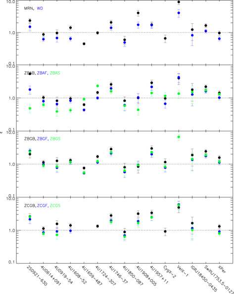
Figure 8. Ratio of the empirical and theoretical values of τsca(2.5 keV)/AV from each source for each model. The dotted line indicates unity.
Download figure:
Standard image High-resolution image6. DISCUSSION
6.1. Unsuccessful Halo Fits
Eight LOS had dust halos that could not be fit with any model. An in-depth analysis of these halos is beyond the scope of this work, but they are each discussed generally below; some are known to have unusual dust properties, while others are not. Nonetheless, it is interesting to contrast these sources with the ones with successful fits. The scale heights of the objects with successful fits varied between ∼40 and 3000 pc. Ten were in the thin disk ( 330 pc, Chen et al. 2001) where most of the dust is. Of these 10, eight were relatively nearby, with
  5 kpc. Twelve well-fit sources had
  330 pc; of these, 11 had
  5 kpc. In contrast, seven of the eight sources with unsuccessful fits had
  5 kpc, and seven were to sources where all or most of the sight line passed through the thin disk. Thus, halos tended to have successful fits when (a) the sight lines were short, or (b) the sight lines were long, but to sources that were out of the Galaxy's plane. Halos around sources that were both distant and in the thin disk usually could not be fit, suggesting that either the dust does not have properties similar to those described in the models, or the cloud distribution is not well described by those used here. We describe these sources in more detail below.
GRS 1915+105 is a low mass X-ray binary and a known Galactic microquasar. The system is composed of a 14 ± 4  black hole and a K-M III companion (Greiner et al. 2001). It has notably variable X-ray emission; Greiner et al. (1996) examined several RXTE observations taken between 1996 February and 1996 June, and found that its brightness varies on timescales ranging from seconds to days. GRS 1915+105 lies in the plane of the Galaxy (
 ) at a distance of ∼9–12.5 kpc (Mirabel & Rodriguez 1994; Fender et al. 1999; Dhawan et al. 2000; Chapuis & Corbel 2004). Chapuis & Corbel (2004) used radio and millimeter observations to measure NH along the LOS, and thus the optical extinction AV. They found NH = (3.5 ± 0.3) × 1022 cm−2, which agrees with our value of (3.43 ± 0.03) × 1022 cm−2, which was derived from the X-ray spectral fit. They note that an AGB star is only 18'' away, and place it at a maximum distance from the Sun of about 6 kpc. Such stars can eject material up to 1 pc, or 36'' on this scale. For the halo to be free of any effect from the AGB star, the inner radius of the halo measurement must be greater than 54''. The halo was fitted from 50 to 800''. Out of an abundance of caution, we checked for any influence from the AGB dust by refitting it from 60 to 800'' for the MRN model, using both the single-cloud and smooth distributions. The results were not significantly different from those obtained when fitting from 50 to 800'', so we believe that the halo fits are minimally influenced by the AGB's ejecta.
4U 1538–52 (QV Nor) is a well-studied eclipsing high mass X-ray binary system composed of a pulsar and a highly reddened ( ) B0Iab companion (e.g., Crampton et al. 1978; Pakull et al. 1983; Reynolds et al. 1992). The dust along this LOS has also been examined in detail (Clark et al. 1994; Clark 2004), with the result that the halo can be fit when the source is at 4.5 kpc and there are three MRN-like clouds, two at distances corresponding to concentrations of atomic H, and the third closer to the source. Our attempts to reproduce this result were not sucessful. It has also been suggested that the halo intensity is less than expected given the B0Iab's extinction, leading to the suggestion that it may exhibit porous dust (Clark et al. 1994). However, as discussed in Section 6.2, the results of the present work indicate that porous grains are not required to fit halos.
4U 1820–30 (Sgr X-4) is a low mass X-ray binary in the globular cluster NGC 6624, at a distance of about 8 kpc (Harris 1996, 2010 edition). It is an intriguing system, and has been the subject of many studies. It is composed of a neutron star primary with an He-rich white dwarf companion that has filled its Roche lobe. Of all known binaries with a neutron star or black hole primary, it is the most compact, having an orbital period of 11.4 minutes (Stella et al. 1987; Chou & Grindlay 2001). It has been suggested that this system formed through a collision between the neutron star and a giant, which has since lost its outer layers to mass transfer so that all that remains is its He-rich core (Verbunt 1987; Ivanova et al. 2005). An additional periodicity in the system's luminosity suggests the presence of a third body in the system, orbiting the neutron star-white dwarf inner binary (Zdziarski et al. 2007; Wang & Chakrabarty 2010). The IS medium along this LOS has been examined by Costantini et al. (2012), who studied absorption features in its soft X-ray spectrum and found a slight overabundance of O and underabundance of Fe (with respect to the solar nebula values of Lodders & Palme 2009).
XTE J1720–318 (V1228 Sco) is a low mass X-ray binary that is believed to harbor a radio-quiet black hole. It was examined in detail in the optical and near-IR by Chaty & Bessolaz (2006), who determined that the companion is most likely a main-sequence star, with spectral type ranging from late B to early G. They found that the system is likely at a distance of 3–10 kpc. Values for AV range from about 6 to 8 mag (Nagata et al. 2003).
IGR J17544–2619 is a super fast X-ray transient that was discovered in 2003 (Sunyaev et al. 2003). Data taken during an outburst in 2004 clearly show a complicated time-dependent halo structure, an examination of which suggests that there are two clouds along this sight line (Mao et al. 2014).
GX 13+1 is a low mass X-ray binary with a neutron star primary. Bandyopadhyay et al. (1999) determined the companion star to have spectral type K5III, and placed the system at a distance of 7 kpc in the Galactic bulge. The NH found for the source, (2.75 ± 0.06) × 1022cm−2, is slightly lower than that found by Ueda et al. (2004; NH =  cm−2) and implies an optical extinction of ∼15 mag. Smith (2008) examined the halo using simultaneous RXTE and Chandra HRC-I data and could not find a dust model that fit adequately.
GX 5–1 is a heavily absorbed ( cm−2) low mass X-ray binary near the Galactic Center. In Smith et al.'s (2006) examination of its halo using Chandra ACIS data, they found that the single-cloud distribution was more successful than a smooth distribution, as seen in this work. However, they also found that their best-fit model, ZBGB, had
  in the E = 2.4–2.6 keV band. This contrasts with the fits from this work, all of which had values of
  around this energy and differences between the fits and the data that were larger than 3σ. The broader bandpass used in this work and the extreme brightness of the source are likely the cause of the discrepancy.
4U 1119–603 (Cen X-3) is a high-mass X-ray binary is composed of a neutron star and O6 II, at a distance of about 6–8 kpc. Its dust halo was examined by Thompson & Rothschild (2009), who used data from the Chandra HETG to fit its halo over radial distances from the source <100''. In contrast, in this work, data from XMM's MOS camera were used over a much larger radial extent (<600''). They found that a good fit was provided using four clouds of WD-type dust. Our attempts to reproduce this result were not successful.
6.2. Porosity
Porous conglomerate (silicate+carbonaceous) grains were proposed by Mathis & Whiffen (1989) to be a more realistic grain population than two seperate populatons of pure graphite and silicate, as proposed by MRN. Porous grains also are more efficient scatterers and absorbers at UV/optical wavelengths than non-porous (compact) grains, and so may help to solve the problem of having IS abundances that were too low to account for IS extinction (Mathis 1996), although this is not undisputed (Li 2005). In X-rays, porous grains are less efficient scatterers than compact grains, so if there are porous grains in the ISM, halo fits using models that do not explicitly contain them should produce values of τsca that are lower than expected for a given AV. The potential detection of porous grains in the ISM has been controversial. Woo et al. (1994) found that the halo of Cen X-3 could be fit with MRN when the grains were ∼50% porous. Similarly, Predehl & Schmitt (1995) fitted their halo sample with variants of the MRN PL grain size distribution ( , solving for q and maximum radius amax) and found values of q and amax that were similar to those of the standard MRN, though they also calculated that for grains with radius = 0.1 μm, if the grain-forming elements are largely depleted, then grains must be up to 70% voids in order to not exceed the observed halo intensities.
However, these works examined halos at low energies ( keV) and relied on the RG approximation of the differential scattering cross section. Smith & Dwek (1998) showed that Rayleigh–Gans substantially overestimates halo intensity at these energies, compared to results from the Mie solution. Further, they assume cosmic abundances that are much higher than are currently indicated. For instance, Predehl & Schmitt (1995) relied on the work of Morrison & McCammon (1983), whose cosmic abundances are notably higher than those of more recent works (e.g., Nieva & Przybilla 2012). If ISM abundances are indeed much lower, fewer voids are needed to avoid overly bright halos (Mathis 1996).
Our results indicate that porous grains are not necessary to fit halos. They do this in two ways. First, the models that contain them (the ZDA COMP- families) performed markedly worse than those without, as can be seen from Table 14, where the number of sources a model could fit is listed. Second, of the models that did not have porous grains (MRN, WD, and the ZDA BARE- families), values of τsca/AV were similar to their expected theoretical values with  . Halo intensity depends strongly on grain size, so the general ability or inability of a model to fit a halo relies heavily on the large end of its grain size distribution. The most successful models (MRN and ZDA BARE-) had similar maximum grain sizes,
  0.25–0.4 μm, which were notably smaller than those of the less successful ones, which had amax = 0.5–0.9 μm.
Successful models also had fewer large grains, which can be seen in ZDA's Figures 4–17. The number of large grains a model had tracked closely with its halo fitting success. Of the models tested here, the COMP-AC family had the most large grains. COMP-GR-FG and COMP-GR-S had fewer, and the BARE- family had the least. The large end of the grain size distribution of the COMP-GR-B model was more similar to that of MRN and the BARE- families, although amax was larger (0.52 μm); it was also the most successful member of the COMP- family. WD does not contain porous grains, but its large grain size distribution is comparable to that of the COMP- family, so it is not surprising that it performed in a similar way. Dwek et al. (2004) also noted that the BARE- models tended to fit halos better than COMP- models, again, because of the grain size distribution.
Of course, these results do not completely exclude the possibility of porous grains; they only place limits on how large they (and compact grains) can be, and how many there are. It seems unlikely that very large grains ( m) are present in any significant quantity in the diffuse ISM or most cold clouds.
6.3. Non-uniform Halos?
As noted in Section 5.4, some models produced scattering optical depths that were larger or smaller than expected for the sight lines' optical extinctions. After verifying the values of AV in the literature, possible issues with the empirical values of τsca(2.5 keV) were considered. If the source is projected near a region of ISM that is not uniform (for example, near the edge of an intervening cloud), it is possible that the AV that is measured on the source's LOS is not consistent with the τsca in different regions of the halo. In that case, one might expect that  only for parts of the halo.
To investigate halo non-uniformity, all halos were divided into quadrants according to Galactic latitude and longitude. This is a similar approach to that used in the detailed study of halo azimuthal variation by Seward & Smith (2013), although the detailed data used in their analysis was not available here. Only the sources with at least 3,000 counts in each quadrant were analyzed further to ensure a solid measurement of τsca. Six sources met this requirement in the E = 2.5 keV bandpass; Vel X-1 did not, but it did in the E = 4.0 keV bandpass, so that band was used instead. These bright quadrants were then fitted with the MRN model, and was found. These are listed in Table 16, along with the standard deviation from the mean of the quadrants, and the number of models for which these halos deviated from their expected values by more than a factor of two when the entire halo was fitted. (Again, the 4.0 keV bandpass was used for Vel X-1.) Several points are of note.
Table 16.
Values of  for Sources With >3000 Counts per Quadrant
| Source | Quadrant | Quadrant | Quadrant | Quadrant | Standard | No. of Models With |
|---|---|---|---|---|---|---|
| 1 | 2 | 3 | 4 | Deviation | Discrepant 
|
|
| 4U 1608–52 | 1.68 ± 0.24 | 0.96 ± 0.14 | 1.00 ± 0.14 | 1.80 ± 0.26 | 0.4 | 0 |
| Cyg X-2 | 2.27 ± 0.31 | 1.10 ± 0.17 | 1.67 ± 0.24 | 1.33 ± 0.19 | 0.5 | 0 |
| 4U 1659–487 | 1.45 ± 0.12 | 0.49 ± 0.04 | 0.53 ± 0.06 | 1.35 ± 0.11 | 0.5 | 2 |
| Vel X-1 | 3.38 ± 0.49 | 6.49 ± 0.90 | 7.53 ± 1.04 | 1.98 ± 0.30 | 2.6 | 11 |
| Swift J1753.5–0127 | 1.44 ± 0.38 | 11.5 ± 1.4 | 8.32 ± 1.04 | 12.7 ± 1.5 | 5.1 | 2 |
| 4U 1957+11 | 16.7 ± 3.4 | ⋯ | 1.31 ± 0.29 | 3.69 ± 0.76 | 7.5 | 7 |
| 4U 1746–37 | 41.7 ± 6.3 | 35.3 ± 5.4 | 6.96 ± 1.21 | 3.50 ± 0.67 | 19 | 6 |
Download table as: ASCIITypeset image
First, some sources show large differences between the  found for each quadrant, often having the expected
  for one or two quadrants, and an
  that was significantly larger or smaller for the remainder. This suggests that the AV on the source's LOS is consistent with the τsca only for parts of the halo. Second, sources with larger deviations between quadrants were more likely to have empirical values of τsca(2.5 keV)/AV from the whole-halo fits be significantly different from their theoretical values. It is interesting to consider that the source with the highest deviation, 4U 1746–37, is in a globular cluster that is known to have differential Galactic reddening with
  over its central 200'' (see Section 5.1). In this work, the halo was examined over an angular distance of 600'', with the regions of highest [τsca(2.5 keV)/AV]empirical corresponding to quadrants that were closest to the Galactic plane. For 4U 1957+11, which had the second highest deviation between quadrants, the reddening of several stars within an 800'' radius was found to range from ∼0.1 to 0.5. Vel X-1 had only a modest deviation, but the largest number of discrepant
  values; in the 4.0 keV band, no model could produce [τsca/AV] within a factor of two of the expected value. This source is located in the Vel OB1 association, which has reddening that ranges between 0.3 and 1.4 (Reed 2000). An image of Vel X-1 made with the DSS and Wide-field Infrared Survey Explorer (WISE) 12 and 22 μm survey data is shown in Figure 9. An arc-shaped region of emission is clearly visible, at a distance of about 50'' from the source, as is patchy nebulosity over the entire region. If such a structure is also associated with X-ray-scattering dust in the region of halo extraction, it supports the possibility that inhomogeneities in the ISM give rise to discrepant halos. In contrast, sources with lower deviations and fewer discrepant values had a narrower range of reddenings: within 800'' of Cyg X-2, 4U 1608–52, and 4U 1659–487, E(B–V) ranged from
  ,
,  , and
, and  , respectively.

Figure 9. Sky near Vel X-1. Data from the Digitized Sky Survey is in blue, the WISE12 μm and 22 μm All-Sky Surveys are in green and red, respectively. The two white circles indicate the halo extraction range, and the quadrants used in Section 6.3 are shown.
Download figure:
Standard image High-resolution image7. CONCLUSIONS
Our results may be summarized as follows:
- 1.The ratio of AV/NH (1021 cm−2), as determined from the X-ray spectral fits to X-ray binaries, is
 . This is in agreement with that found by Güver & Özel (2009) for SN remnants and similar to that found by other workers both in the X-ray and UV regimes.
 - 2.Out of 35 sources with halos that could be detected, 27 could be fit by one or more dust models considered here. The models that produced the most sucessful fits were MRN and the ZDA BARE- models, fitting 26–27 sources. In contrast, the ZDA COMP- models were less successful, producing acceptable fits to only ∼10–20 sources. The key difference is due to the halo intensity's dependence on the large end of grain size distribution, as only small changes in the grain sizes or number of large grains is enough to notably change a model's ability to fit a halo. Neither the diffuse ISM nor most cold clouds contain a significant presence of grains with 0.5 μm, regardless of their porosity.
- 3.Of the 27 sources that could be fit, the single dust cloud distribution consistently produced better fits than the smooth dust distribution.
- 4.Eight sources could not be fit with the models considered here. Some of these are known to have unusual dust along their sight lines, whereas others are not. Whether or not a halo could be fit tended to depend on if the sight line traversed a long distance through the Galactic plane. Successful fits were produced when either the sight lines were relatively short ( 5 kpc), or the sight lines were long ( 5 kpc) but to sources that were out of the Galactic thin disk, which is where most of the dust is. Sources that were both in the thin disk and distant could not be fit, possibly because there were more intervening clouds than accounted for here, or the grains on those sight lines are not well described by the models.
- 5.Some sources had good halo fits that had values of τsca/AV that were notably different from their expected theoretical values. By dividing sufficiently bright sources into quadrants and fitting those halos, it is possible to detect differences between quadrants among the discrepant halos that are not seen in the quadrants of the halos that produced τsca/AV similar to their theoretical values. The discrepant halos covered regions on the sky that had a broader range of E(B–V) than non-discrepant ones. Further, it was noted that Vel X-1, which had the highest number of models that produced τsca/AV that deviated from the expected values, is located near an arc-shaped region of IR emission. This supports the suggestion that inhomogeneities in the ISM may account for these discrepant halos.


The authors thank the anonymous referee for many insightful comments that significantly improved this work. They also gratefully acknowledge helpful discussions with Eli Dwek and Fred Seward. Financial support for this work was made possible by NASA Grants NNX10AE04G and NNX10AD10G and Chandra grant GO7-8142B.
Facilities: CXO - Chandra X-ray Observatory satellite, XMM-Newton - Newton X-Ray Multimirror Mission satellite.
Footnotes
- 4
- 5
- 6
- 7
- 8
- 9
- 10
- 11