


Abstract
This paper describes the enhanced pedestal (EP) H-mode observed in the National Spherical Torus Experiment (NSTX). The defining characteristics of EP H-mode are given, namely (i) transition after the L- to H-mode transition, (ii) region of very steep ion temperature gradient, and (iii) associated region of strong rotational shear. A newly observed long-pulse EP H-mode example shows quiescent behaviour for as long as the heating and current drive sources are maintained. Cases are shown where the region of steep ion temperature gradient is located at the very edge, and cases where it is shifted up to 10 cm inward from the plasma edge; these cases are united by a common dependence of the ion temperature gradient on the toroidal rotation frequency shear. EP H-mode examples have been observed across a wide range of q95 and pedestal collisionality. No strong changes in the fluctuation amplitudes have been observed following the EP H-mode transition, and transport analysis indicates that the ion thermal transport is comparable to or less than anticipated from a simple neoclassical transport model. Cases are shown where EP H-modes were reliably generated, though these low-q95 examples were difficult to sustain. A case where an externally triggered edge localized mode (ELM) precipitates the transition to EP H-mode is also shown, though an initial experiment designed to trigger EP H-modes in this fashion was unsuccessful.
Export citation and abstract BibTeX RIS
1. Introduction
1.1. Motivation
The spherical torus (ST) [1] has the potential to provide the fusion core for a number of next-step fusion missions. These include devices to prototype nuclear technologies for devices to prototype nuclear technologies for demonstration power plants [2–6], fusion pilot plants [7], and full fusion reactors [8, 9]. These studies often invoke a level of energy confinement well beyond that projected by the ITER-98(y,2) scaling expression [10]. For instance, a recent pilot plant study [7] found that a confinement level specified by H98(y,2) = 1.3−1.35 was desirable, while the reactor study in [9] specified H98(y,2) = 1.6. The component test facility (CTF) [11] and fusion nuclear science (FNSF) facilities described in [2–4, 6] all assume 1.3 < H98(y,2) < 2.1.
Spherical torus H-mode thermal confinement [12] with boronized plasma facing components (PFCs) has shown scalings with IP and BT [13–15] that are significantly different from the ITER-98(y,2) expectation. For instance, from [13], the IP exponent is typically in the range of 0.5–0.6, compared to the ITER-98(y,2) exponent of 0.93. The toroidal field exponent has been found to be ∼0.8–1.1, compared to 0.15 in the ITER98(y,2) expression. However, numerical values of the confinement time are roughly similar to the values from that conventional aspect ratio scaling expression. Furthermore, lithium conditioned H-mode scenarios in National Spherical Torus Experiment (NSTX) showed confinement not significantly different in magnitude and scaling from the ITER-98 expression, though H98(y,2) multipliers up to 1.3 [16] have been observed with strong lithium conditioning of the PFCs [17, 18] (note that the confinement in NSTX has generally been observed to increase with the level of lithium conditioning) [19, 20]. Hence, while H-mode thermal confinement values in the ST can be comparable to that in conventional aspect ratio devices, reliable access to the confinement regimes anticipated for next-step devices is not assured.
Various regimes with enhanced confinement compared to H-mode have been observed in conventional aspect ratio tokamaks. For instance, internal transport barrier plasmas [21] can have substantially higher levels of stored energy than comparable L-mode discharges. Enhanced edge transport barriers have also been observed in the form of the VH-mode [22–28]. Both of these regimes have produced confinement multipliers H98(y,2) approaching or exceeding two. Internal transport barrier regimes have been accessed in NSTX [29, 30] with high harmonic fast wave (HHFW) heating [31], though the L-mode edge results in reduced global confinement and undesirable stability properties. While the VH-mode itself has never been observed in a spherical torus, a different regime of enhanced confinement at the plasma edge has been observed. It is the purpose of this paper to discuss this regime, known as the enhanced pedestal (EP) H-mode.
1.2. Definition of the EP H-mode
The EP H-mode [32, 33] is an enhanced confinement regime in NSTX characterized by the following features:
- There is a transition to the EP H-mode from the normal H-mode phase. Transitions from L-mode directly to EP H-mode have not been observed. This transition to EP H-mode is typically triggered by some external event such as an ELM.
- There is a region towards the edge of the plasma where the ion temperature gradient is much steeper than in standard H-mode. This is illustrated most clearly in figure 1, where the maximum absolute value of the Ti gradient at the outboard midplane is plotted as a function of plasma current. This maximum gradient is determined by fitting a line to sets of four adjacent charge exchange recombination spectroscopy (CHERS) channels, with the error bars determined by the uncertainty in the fit parameters given the uncertainties in the individual Ti measurements. This process is repeated across varying sets of four channels across the plasma edge to determine the largest local gradient. The blue points are taken from the EP H-mode phase of the discharge, and show substantially higher Ti gradients than in the H-mode phases in red.
- The region of steep Ti gradient coexists spatially with a region of strong rotation shear. There is often a local minima in the rotation in this region, though that is not a strict requirement for the identification of the regime.

Figure 1. Maximum ion temperature gradient for EP H-mode (blue) and H-mode (red) examples in NSTX. The difference between squares and diamond symbols will be described in section 3. The database analysis that produced this plot will be described in more detail in section 4. The discharge numbers refer to discharges that will be discussed in detail in this paper.
Download figure:
Standard image High-resolution image1.3. Overview of this paper
This paper provides an overview of EP H-mode observations from NSTX. Section 2 provides additional general characteristics of the EP H-mode, while section 3 describes the typical profile shapes and evolution. Section 4 presents database analysis of EP H-mode examples in NSTX. Section 5 describes measurements of turbulent fluctuations and transport analysis. Section 6 describes attempts to control the EP H-mode transition and subsequent evolution, while section 7 provides some conclusions.
1.4. Description of the NSTX device
NSTX [34] is a medium sized spherical torus device located at Princeton Plasma Physics Laboratory. Plasmas typically have a major radius of 0.9 m, and a minor radius of 0.6 m. Toroidal fields strengths for typical discharges are in the range 0.35 < BT(T) < 0.55, with typical plasma currents for H-mode discharges in the range of 600 < IP(kA) < 1200. All plasmas described in this paper are heated by neutral beam injection in the direction parallel to IP, with up to 7 MW available [35]. HHFW heating is also available [31], though it was not utilized for these plasmas.
NSTX plasmas are assessed with a comprehensive set of diagnostics. The electron temperature and density profiles are measured with a multi-pulse Thomson scattering (MPTS) diagnostic [36]. The impurity ion (C6+) temperature, density, and toroidal rotation are measured by a charge exchange recombination spectroscopy (CHERS) system [37], with an averaging time of 10 ms per sample. The magnetic field pitch angle is measured with a motional Stark effect (MSE) polarimetery system [38], and, when available, is used to constrain equilibrium reconstructions with the LRDFIT code [39] on a case-by-case basis. Routine magnetohydrodynamic (MHD) equilibrium reconstructions with the NSTX implementation [40, 41] of the EFIT code [42] are also available and used in this analysis; note that these routine post-shot reconstructions are not constrained by MSE measurements.
2. General characteristics of EP H-mode
The temporal characteristics of EP H-modes in NSTX can roughly be divided into two groups. The first group contains high-current cases which transition to this confinement regime at the end of the IP ramp or early in the IP flat-top. The current profile is typically rapidly evolving in these cases, and the EP H-mode phase is typically of limited duration due to disruptions or transition back to H-mode. The second group contains cases that transition to EP H-mode much later in the IP flat top. These cases have demonstrated the highest confinement and longest pulse of all EP H-mode examples observed to date.
2.1. Examples of the early-transition EP H-modes
The first EP H-mode plasmas observed in NSTX had comparatively short durations of the steep ion-temperature gradient [32], and were typically observed early in the discharge in higher-current plasmas. Two examples of this sort of discharge are shown in figure 2. The quantities illustrated are indicated in the figure caption, with some clarification required for the stored energy traces in figure 2(c). The solid line in that frame corresponds to the stored energy calculated from the MHD equilibrium reconstruction with the LRDFIT code, while the dashed lines are from interpretive TRANSP [43] simulations. The stored energy in this simulation is the sum of the thermal energy (indicated in the dotted line) and the fast ion stored energy, as computed by NUBEAM [44].

Figure 2. Time evolution of short-lived EP H-mode example discharges. Shown are (a) the plasma current and beam power, (b) the divertor Dα emission, (c) the stored energy, (d) the line averaged density and (e) the odd-n MHD trace, indicative of n = 1 rotating kink/tearing modes.
Download figure:
Standard image High-resolution imageIn these examples, which came from two different run campaigns, the plasma current ramps to IP = 1200 kA, with the full 6 MW of neutral beam heating power applied by the time the current has reached 700 kA. The plasmas transition to H-mode at t = 0.13 s (141340) and t = 0.15 s (138219). A large ELM then occurs (see figure 2(b)), which triggers the transition to EP H-mode. This transition is indicated by the dashed vertical lines in all frames. The stored energies then begin to ramp, with the dominant effect being an increase in the thermal stored energy. As will be shown in section 3, there is a remarkable steepening of the edge ion temperature gradient during the EP H-mode phase. In these cases, the line-average density stays approximately fixed during the EP H-mode phase. In both cases, a disruption ends the EP H-mode phase, presumably due to the large pressure gradient, however, macrostability calculations for these plasmas have not been systematically attempted.
Examples like these indicate the potential value of the EP H-mode configuration. However, discharges with longer durations are clearly required in order to understand the potential of the regime. The next section discusses discharges of this type.
2.2. Examples of the late-transition EP H-modes
Two examples of more stationary, late-transition EP H-modes are described in this section. Here, the phrase late-transition refers to cases where the transition occurs well after the current ramp is complete. Time traces from these discharges are shown in figure 3, where the individual frames are largely similar to that in figure 2. The most significant difference is in frame (e), which shows the current in one of the radial field coils. The more rapid dynamics in this coil are typically driven by the shape and vertical position control feedback loops; the significance of this waveform will be made apparent in later discussion. Figure 4 illustrates the boundary shapes for these two discharges during their EP H-mode phases.
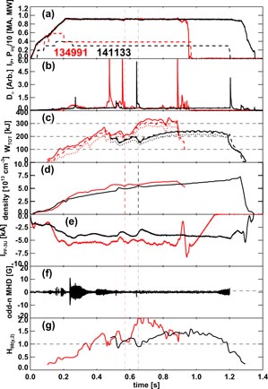
Figure 3. Time evolution of long-pulse EP H-mode example discharges. Shown are (a) the plasma current and injected neutral beam power, (b) the divertor Dα emission, (c) the stored energy, (d) the line-average density, (e) the current in the radial field coil, (f) the odd-n rotating MHD signal (141133 only), and (g) the H98(y,2) confinement multiplier. See text for additional details.
Download figure:
Standard image High-resolution image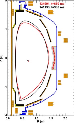
Figure 4. Typical separatrix shapes for the long-pulse EP H-mode examples in figure 3.
Download figure:
Standard image High-resolution imageDischarge 134991 was described in [33], and represented the longest-duration EP H-mode discharge at the time. This 900 kA discharge from the 2009 campaign was made during an experiment to develop scenarios for experiments with the liquid lithium divertor (LLD) [45] in 2010. As part of this development effort, strike-point controllers [46, 47] were being developed, and super sonic gas injection [48] was being used to supplement the standard low-field and high-field side [49] fuelling. A large ELM at t = 0.555 s triggers the transition to EP H-mode. This results in an increase in the global confinement, with the stored energy ramping from ∼210 to ∼320 kJ. This high-performance phase lasts approximately 300 ms, or 2–3 confinement times, before a disruption occurs.
The second discharge in the figure (141133) was observed as part of the database study reported in section 4. As can be seen in figure 4, this is a high-elongation and triangularity discharge typical of the highest performance NSTX discharges [15, 50], without feedback control of the strikepoints. In this case, a small ELM at t = 0.5 s triggers an apparent transition to EP H-mode. A second ELM occurs at t = 0.65 s, leading to a large stored energy loss. However, the plasma recovers into EP H-mode once more. The stored energy ramps to ∼230 kJ, corresponding to H98(y,2) ∼ 1.5. The density ramps throughout the EP H-mode phase in both this and the other discharge in the figure. In both cases, this is due to the accumulation of carbon in the discharge; the deuteron inventory is well regulated, as is typical of discharges with significant lithium conditioning of the PFCs [51]. This discharge is extremely quiescent during the EP H-mode phase, showing no significant dynamics until the heating power is turned off at 1.2 s and the current rampdown is initiated at 1.25 s.
The current in the radial field coil (frame (e)) is shown as a measure of the global quiescence of the discharge. This current is determined entirely by feedback loops for the plasma elongation and vertical position [52]. In particular, discharge 141133 shows almost no variation in this current during the EP H-mode phase, indicating that the configuration is quite steady and free of transients; this level of variation is lower than in typical H-mode discharges, or in discharge 134991 (though it should be noted that the poorly tuned strike-point controllers likely also played a role in the radial field variations in that discharge).
3. Profile variations in EP H-mode
3.1. Overview of the edge pedestal characteristics in EP H-mode
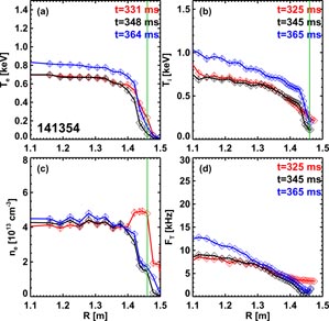
As first described in [32, 33], the EP H-mode phase is characterized by a steep gradient in the ion temperature profile at the edge of the plasma. However, more recent examination of the NSTX database has shown that the exact location of the steep gradient region with respect to the separatrix can vary significantly. This is illustrated in figure 5, where the profiles from three different discharges are plotted in three columns. These profiles are plotted against major radius, so that complications associated with flux-mappings can be avoided. The separatrix location is shown as the gray shaded region for all figures, determined by the values give by equilibrium reconstruction, the Te = 40 eV location, and the Te = 80 eV location.

Figure 5. Examples of profile shapes during EP H-mode in NSTX. The top frame of each column shows the ion and electron temperature profiles. The points show the data, while the red lines show tanh fits to the Ti data, magenta lines mark the location of maximum ion temperature gradient and the tangent line to the profile at that point. The middle frames show the toroidal rotation frequency FT and ER + VPBT profiles, while the bottom frames show the electron and carbon density profiles. The grey shaded regions indicate the approximate regions of the separatrix. Note that the magnetic axis is typically at R = 1.03 m for these cases. The ellipse in frame (f) indicates a small local flattening of the electron density profile. See text for additional details.
Download figure:
Standard image High-resolution imageIn this figure, the top row shows the electron and ion temperatures, along with both tanh fits to Ti and a line tangent to the point of the maximum Ti gradient. The tanh fit in this and other figures is defined via the function:

with z = 2(Xsymmetry − X)/Δwidth [53]. Here, Y can represent Te, Ti, ne or any other profile quantity, while X can represent either outboard midplane major radius or some flux surface label such as normalized poloidal flux. Yoffset, Ypedestal, αslope, Xsymmetry, and Δwidth are fit parameters determined by a non-linear fitting routine [54].
The second row shows the toroidal rotation profile (here, indicated by the rotation frequency FT in kHz), as well as the quantity
 . The poloidal rotation is generally small in NSTX [55], and so the VPBT term may not be a significant contributor to this calculation; this was previously found to be the case for discharge 134991 [33]. However, because it has not been assessed across this wider range of EP H-mode cases, it is not possible to systematically neglect it with high confidence. The bottom row shows the electron and scaled carbon density profiles, along with spline fits to those profiles.
The left-most column of figure 5 shows the edge profiles for the long-pulse EP H-mode discharge 134991, whose time evolution is illustrated in figure 3. In this case, the region of steep Ti gradient is very close to the plasma edge. There is a clear minima in the rotation profile, with a deep ER well developing. The profiles for the other long-pulse discharge in figure 3 (141133) are of similar shape, and will be illustrated below.
The middle column of figure 5 shows the profiles for a case typical of the short-lived EP H-modes that transitions before or just after the start of the IP flat-top; see figure 2 for the time evolution of 0D quantities in this case. In this example, the region with the steepest Ti gradient is shifted in a few cm, with a clear region of lower Ti gradient farther outside. However, the rotation profile minima and ER well are still present. Note that these profiles are not maintained in steady state; the disruption follows soon after the time shown in the figure.
Finally, the right most column shows a case where the steep Ti gradient is shifted inward ∼10 cm from the plasma edge. There is an associated inward shift of the region of sharp rotation gradient indicating that the relationship between the steep ion temperature gradient and rotation is maintained. In this case, both Te and ne show a double-barrier structure, and the configuration could be called a wide radius internal transport barrier (ITB) as well as an EP H-mode. For this reason, cases such as in the right column of figure 5 are noted with squares in the scatter plots below and in figure 1, whereas cases such as in the left and centre column will be denoted with diamonds.
3.2. Time evolution of the edge pedestal following the transition to EP H-mode
The data in figure 5 provide a clean indication of the different profile shapes in EP H-mode, but do not provide information on the time evolution to those profiles. Hence, section 3.2 provides information about that evolution.
The profile evolution for the example in the centre column of figure 5 (discharge 141340) is shown in figure 6; this is the high-current example transitioning to EP H-mode early in the discharge. The CHERS data (FT, Ti, ER) and MPTS data (Te, ne) are on slightly different time bases, so nearly synchronous samples are indicated with the same colour; also recall that the CHERS data is averaged over 10 ms windows. At t = 330 ms, the configuration is in H-mode, with relatively broad density, temperature and rotation profiles. The bottom of the Ti pedestal is not resolved by the CHERS diagnostic for this time slice due to the low edge electron temperature, and so the ER features at the edge are not fully resolved.
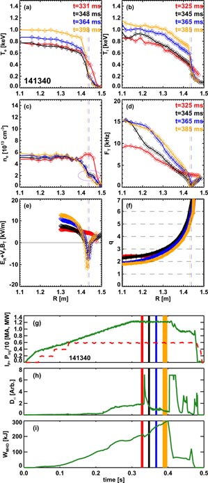
Figure 6. Profiles and waveforms for a typical early-transition EP H-mode example 141340. The upper frames show the time evolution of the profiles of the (a) electron temperature, (b) ion temperature, (c) electron density, (d) toroidal rotation frequency, (e) radial electric field (formally, ER + VPBT), and (f) safety factor (q). The bottom frames show the time evolution of the (g) plasma current and heating power, (h) divertor Dα, and (i) total stored energy. The vertical bands in (g)–(h) indicate the ranges of time for the profiles plotted in (a)–(f). The dashed vertical lines in frames (a)–(f) indicate the location of the rotation minima for selected times.
Download figure:
Standard image High-resolution imageAfter t = 340 ms, the EP H-mode transition occurs following a large ELM, with a number of associated changes in the profiles. The electron density and temperature at the plasma edge are reduced following the ELM, and the rotation immediately develops a local minima. The ion temperature at the very edge is also transiently reduced, though the core ion temperature is largely unchanged; this results in a region of sharp Ti gradient at the location where the two regions connect. These rotation and pedestal dynamics result in the formation of a deep well in the ER profile. Indeed, both the magnitude and spatial scale of the large ER shear region is significantly larger in the EP H-mode phase than in the H-mode phase [33].
From that point onward, the minima in the rotation remains, marked by vertical dashed lines in the figure for the later time slices. The width of the ion temperature pedestal increases at roughly fixed gradient scale length until the EP H-mode phase ends with a disruption. Note the apparent local flattening of the density profile, barely visible in the bottom centre frame of figure 5, but clearly visible in figure 6(c) within the magenta oval.
It has been speculated that the minima in the rotation profile is associated with a single rational surface [33]. However, as illustrated in figure 6(f), isolating which surface would play this role has proven difficult. This frame shows the q profile at the time of interest, with the horizontal lines indicating where a rational surface might be anticipated. The minima in the rotation appears to not be located at the q = 2, 3, or 4 surfaces. It may be located at one of the q > 4 surfaces, though isolating which one is essentially not possible due to the large magnetic shear. Alternatively, as discussed in section 7, it is possible that 3D effects are present that render this mapping more difficult to interpret. Also note that there are some rotating n = 1 MHD modes present during the EP H-mode phase; these are visible in figure 2(e). However, these modes have decreased in amplitude by the time the EP H-mode transition occurs. Inspection of the spectrograms shows that these modes have frequencies of ∼5 kHz during that phase of the discharge, which is clearly well above the frequency of the minima in the rotation, and implies that they are not directly responsible for the rotation minima.
Figure 7 shows similar profile information, for the long-pulse quiescent EP H-mode scenario in discharge 141133 (see figure 3). Similar dynamics can be observed in this example, with the ELM at t = 0.640 s leading to a substantial loss of the edge electron (frame (a)) and ion temperatures (frame (b)), as well as of the toroidal rotation frequency (frame (d)). In this case, it appears as if the plasma may have been in a weak EP H-mode before the ELM at t = 0.51, so the ER shear is already rather strong before that ELM. However, because the Ti gradient is closer to the edge in this case, the full gradient is not resolvable (the bottom of the Ti gradient is in a region with too low electron temperature to fully ionize carbon). No minima in the rotation frequency profile is visible during the EP H-mode phase except for the time slice at t = 0.845 s, though this may be due to the limited measurement range of the CHERS diagnostic in this case. As is evident in figure 3(f), the EP H-mode phase has no low-frequency n = 1 modes until a small n = 1 mode begins to grow at 1.15 s. Inspection of the complete magnetic spectrogram shows that there are no macroscopic MHD modes present during the bulk of the EP H-mode phase, indicating that large rotating low-n magnetic islands are unlikely to play a significant role in the rotation dynamics.
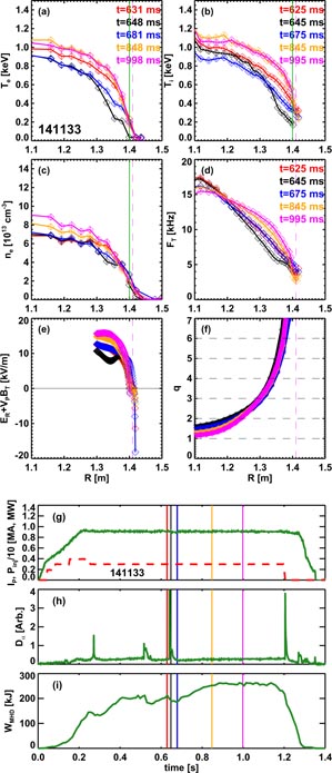
Figure 7. Profiles and waveforms for the long-pulse quiescent EP H-mode case in figure 3 (141133). The frames show the same quantities as in figure 6. The green vertical line indicates the location of the beam emission spectroscopys measurements presented in figure 13.
Download figure:
Standard image High-resolution imageFinally, figure 8 shows the profile evolution for the case with the region of steep Ti gradient shifted substantially inward. In this case, an ELM at t = 0.415 s appears to drive the transition. As with the case in figure 6, that ELM results in a substantial drop in the edge ion temperature, with the perturbation in this case penetrating to R = 1.37 m and leading to increased Ti gradient at that location. The ion temperature outside this radius then stays at the lower value, while the value inside the vicinity of that radius grows to much higher values than before the ELM. This case develops very clear double-barrier structures in the electron density and temperature profiles, with the ne barriers separated by 8–10 cm (note that the minor radius is typically ∼60 cm for these plasmas). There is no minimum in the toroidal rotation frequency, but rather an inflection point at the location of the steep Ti gradient. Note that this inflection point is in vicinity of the q = 4 surface, though there is no indication in the rotation profile of a magnetic island at that location (the plasma maintains a rotation frequency of ∼5 kHz at this location). Also note that the ELMs in this discharge were themselves triggered by impulsively applied 3D fields [56–58]. EP H-modes triggered in this fashion will be discussed in section 6.2.

Figure 8. Profiles and waveforms for an EP H-mode case with the region of steep ion temperature shifted inward. The frames show the same quantities as in figure 6.
Download figure:
Standard image High-resolution imageIdentification of cases like in figure 8 with EP H-mode may appear problematic, as the steep Ti gradient region is shifted well away from the separatrix. However, the examples in this section show that there is a continuum of profile shapes, from those with the steep Ti region at the very edge to those with that region shifted substantially inward. Under the assumption that the underlying physics has similarities, it will be valuable to consider these cases as different manifestations of similar underlying phenomenon.
4. Database analysis of EP H-modes
As part of this research, a significant effort was put into identifying and analyzing a database of EP H-mode examples. As a first step in this study, all NSTX discharges with particularly steep gradients in the ion temperature were identified via automated analysis. These cases were then individually examined to see if they met the characteristics of the EP H-mode, as defined in section 1. It was this process that identified the long-pulse EP H-mode example 141133 noted in figures 3 and 7. These EP H-mode cases were then incorporated into a more detailed database, which yielded the analysis shown in figure 1 and the remainder of this section.
The detailed EP H-mode database evaluates quantities during high-performance EP H-mode phase, and during the H-mode phase preceding the EP H-mode transition. Equilibrium quantities stored in the database come from reconstructions with the LRDFIT code, as well as the NSTX implementation of the EFIT code. Confinement metrics are extracted from TRANSP runs that use NUBEAM to compute the coupled neutral beam power. Consistency of these data is checked by comparing the measured and predicted neutron emission, and comparing the total stored energy computed by TRANSP (thermal+fast ion energy) and computed by the equilibrium reconstruction codes. Fits to the edge Te and Ti pedestals as a function of major radius with the tanh function are also included in the database analysis. The TRANSP and LRDFIT runs used in this database are shown in appendix.
4.1. Global confinement characteristics
As a first analysis step using this database, the increments in stored energy following the EP H-mode transition were examined to determine if, as anticipated from section 3, the increase in stored energy following the EP H-mode transition is largely in the ion channel. Figure 9 shows the increase in the total ion stored energy in frame (a), and the increase in the electron stored energy in frame (b), as a function of the total energy increase. The total energy increase is calculated from the MHD equilibrium reconstruction (δWMHD), or from the increment of the total thermal energy as computed by TRANSP. Note that the sum of the electron and ion thermal energy increases is essentially equal to the total thermal energy increase (δWe + δWd = δWthermal, δWimpurity being small), but they are not constrained to match the increment of energy from MHD equilibrium reconstruction.
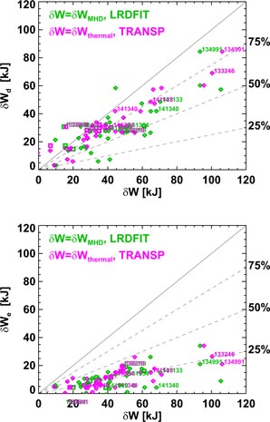
Figure 9. Increments of the deuterium (top) and electron (bottom) stored energy, as a function of the total stored energy increment δ W. The green points are based on calculating δ W from equilibrium reconstruction, while the magenta points are based on extracting δ W from TRANSP runs. Shot numbers are indicated for certain discharges discussed in this paper.
Download figure:
Standard image High-resolution imageThe results of this analysis follow the expected trend. The electron energy increment is typically ∼25% of the total energy increment. However, the increase of deuterium stored energy is typically 75% of the total increase. Hence, physics mechanisms that impact the ion thermal transport are anticipated to be important for determining the characteristics of the EP H-mode.
The confinement multipliers for EP H-modes and the proceeding H-mode phases are shown in figure 10, as a function of q95. Here, the confinement multiplier is defined as H98(y,2) = τE/τ98(y,2). The confinement time is calculated in figure 10(a) as τE = Wth/(Pabs − dWth/dt), with Wth the thermal energy and Pabs the absorbed power. This definition can yield a somewhat noisy evolution of the confinement time due to the time derivative in the denominator, and so the same calculation is shown in figure 10(b), but with the dWth/dt term set to zero. The results are broadly similar, though with some rearrangements of the points and often smaller error bars in figure 10(b).
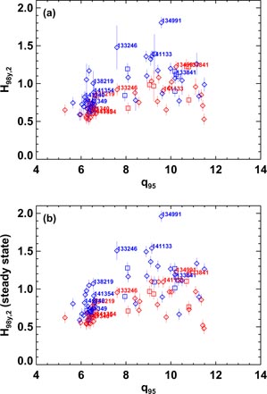
Figure 10. Confinement multiplier as a function of q95 for NSTX EP H-modes. Red points correspond to the H-mode phase of the discharge before the transition to EP H-mode, while blue points are taken from the EP H-mode phase. Frame (a) uses the full definition of the confinement time when calculating H98(y,2), while frame (b) does not correct the absorbed power for changes in the stored energy.
Download figure:
Standard image High-resolution imageThe H-mode phases in these discharges tend to cluster in the range 0.8 < H98(y,2) < 1.0, whereas the EP H-mode cases can have confinement multipliers in excess of H98(y,2) = 1.5. Note the large cluster of data points at q95 = 6. These are the 'early-transition' EP H-modes, many of which come from a dedicated experiment, the results of which are discussed in section 6. As discussed in section 2, these cases tend to disrupt not long after the EP H-mode transition, and so do not achieve the highest levels of confinement. The higher q95 cases often show quite high levels of confinement, aided by the fact that the EP H-mode duration can be longer in these cases. Note that EP H-mode has been observed over a large range of q95.
Additional pedestal parameters are shown in figure 11. In this case, the ion temperature pedestal is fit by equation (1), as a function of major radius; pedestal-top ion temperatures in excess of 1 keV are achievable in EP H-mode. Note that due to the lack to Ti data at the bottom of the pedestal (due to the low electron temperature), tanh fits of single time slices are typically not well constrained in H-mode. As a consequence, Ti,ped is typically not resolvable by these fits, and so no H-mode points are shown here. However, the profiles in figures 6–8 show that the edge ion temperatures are indeed much higher in EP H-mode than H-mode. This result can also be inferred from figure 1, where the maximum Ti gradients are shown in H-mode and EP H-mode.
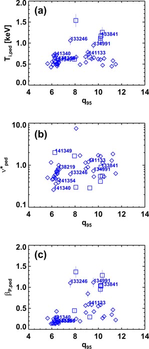
Figure 11. Various quantities versus q95 for NSTX EP H-modes. Shown are (a) the temperature at the top of the ion temperature pedestal, (b) the pedestal-top collisionality and (c) the pedestal βP.
Download figure:
Standard image High-resolution imageThe pedestal collisionality is shown in figure 11(b). Here, the collisionality is defined as
 . The electron density and temperature profiles are sometimes not easily fit to tanh functions. For instance, the multiple gradient region behaviour shown in figures 5–8 can confuse the simple tanh fits. Other times, the use of profile data at a single time results in poor fits (note that recent NSTX pedestal physics studies [53, 59, 60] use a sophisticated set of 'kinetic efit' reconstructions, flux mapping, and conditional averaging technique to improve the quality of the fits using multiple time slices). Hence, Te,ped and ne,ped are derived from the values of their respective profiles, at the radial location of the top of the ion temperature pedestal. In any case, the EP H-mode cases have been observed over a range of pedestal collisionalities, including cases with ve,ped significantly less than unity. Hence, unlike the NSTX type-5 ELM regime [61], the EP H-mode regime is observed to be compatible with low collisionality.
Finally, the pedestal poloidal beta
 value is shown in figure 11(c). Quite high values of this parameter have been achieved, typically in the higher-q95 EP H-mode examples. However, the data does not yet exist to make a systematic study of how the pressure pedestal width scales with βP in these cases, as the single time-slice pedestal fits noted above are incapable of accurately resolving the width due to the lack of points in the pedestal region. Upgrades in the radial coverage of the Thomson scattering system for NSTX-U [62, 63] should improve this situation.
4.2. Relationship between the ion temperature gradient and edge rotation
A previous publication [33] has shown that the pedestal-top ion temperature is proportional to the gradient of the toroidal rotation frequency in EP H-mode. That database consisted of a small number of discharges, all of which had the steep gradient region at or quite near the separatrix. This study has been extended here to a much larger group of discharges, including those with the steep ion temperature gradient locations shifted inward from the separatrix as in figure 8.
As part of this analysis, many different pedestal parameters and rotation metrics were considered, in order to find quantities with the best correlation. With regard to the pedestal performance, both the pedestal height from tanh fits and the maximum ion temperature gradient were considered, and both were taken as the direct value or normalized to the plasma current. One measure of the rotation gradient was taken as the gradient of the rotation frequency (FT) on the small-R side of the rotation minima. Other measures include the rotation difference between the top and the bottom of the Ti pedestal, or the local value of dER/dR.
All combinations of these parameters were plotted, and the plot with the best correlation is shown in figure 12. The vertical axis here is the maximum Ti gradient, normalized by the plasma current. The gradient turns out to be a better indicator of the EP H-mode strength than the pedestal-top temperature, due to cases like in figure 8, where the steep gradient region is shifted in, resulting in a significant vertical offset. The normalization by IP improves the correlation by a small amount, and is roughly consistent with the EP H-mode confinement scaling with IP, though it does not present a conclusive proof of this dependence. The horizontal axis is the simple rotation frequency gradient, as measured on the small-R side of the rotation minima. With this parameter choice, there is a clear correlation between the ion thermal transport and the rotation dynamics. Note especially that the cases with the Ti gradient shifted inwards (indicated with squares) fall in with the cases where the Ti gradient is located much closer to the separatrix, implying that the physics elements may be common.

Figure 12. The maximum ion temperature gradient, normalized to the plasma current, plotted against the radial gradient in the toroidal rotation frequency. Diamonds are for EP H-mode configurations as in figures 5(a) and 5(d), and squares are for configurations as figure 5(g).
Download figure:
Standard image High-resolution image5. Turbulence and transport in EP H-mode
5.1. Observations of turbulence changes across the H-mode → EP H-mode transition
As part of the present EP H-mode studies, an effort was made to examine turbulent fluctuations, to determine if they were reduced during the EP H-mode phase. The primary tool for this study was the beam emission spectroscopy (BES) system [64, 65]. Unfortunately, this diagnostic was available for only a subset of the discharges in this data set. The results of this study are shown in figure 13. Note that the frequency axes are cut off at 100 kHz, as these are the appropriate limits for ion-scale turbulence in the NSTX pedestal [66, 67]. The BES spectra at higher frequencies have been examined, but do not contain any additional information. The top frame in each column also shows the plasma current (yellow) and stored energy (cyan). In each case, the data is shown from the BES chord that intercepts the neutral beam in the steep Ti gradient region; this can be verified by comparing the BES tangency radii given in the top row of figure 13 to the corresponding profiles shown elsewhere in this paper (see the figure captions). However, adjacent BES chords were also inspected, with similar results to those shown here. The vertical lines in the top frame bracket the time windows for the spectrograms in the lower frames. Note that due to the larger discharge duration in the left hand column and the narrow times under consideration (10 ms windows), the bracketing lines appear to blend into a single time for this discharge, while they are distinct for the discharges in the centre and right column.
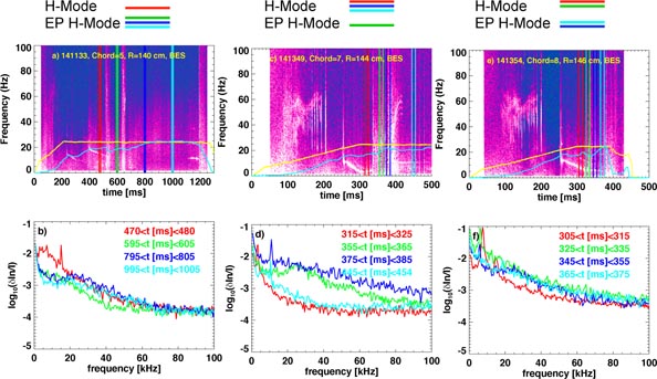
Figure 13. Spectrograms of the BES data for three different discharges. The data in (a) and (b) correspond to the discharge in figures 3 and 7. The data in (c) and (d) correspond to the discharge in figure 18. The data in (e) and (f) correspond to the discharge in figure 14. Figures 7, 14 and 18 have vertical green lines indicating the spatial locations of the measurements. The legend above each column indicates which time slices are in H-mode and which are in EP H-mode.
Download figure:
Standard image High-resolution imageThe left hand column shows BES data for the long pulse example in figures 3 and 7. Spectrograms are plotted for four different times in figure 13(b), with the red times corresponding to the H-mode phase, and the blue and cyan times corresponding to the sustained EP H-mode phase. The green spectrogram is during a short-lived EP H-mode phase. There is no clear sign of a reduction in turbulence during these EP H-mode phases; indeed, one might argue that there is a small increase in density fluctuations during the EP H-mode phase. Note also that there are no clear MHD or turbulent modes located in the pedestal in this EP H-mode example, in contrast to the edge harmonic oscillation (EHO) [68] in QH-mode [68–72], the quasi-coherent mode [73, 74] in enhanced Dα (EDA) H-mode [75], or the weakly coherent mode (WCM) [76] in I-mode [77, 78].
The central column of figure 13 shows the spectra from a discharge that has a short EP H-mode phase, proceeded by and followed by H-mode phases; this discharge will be discussed in section 6. The only spectra from the EP H-mode phase is shown in green, and the fluctuation amplitudes are found to be similar to those in the H-mode phase immediately following the transition back to H-mode (blue spectra). However, the fluctuations in the H-mode phase before the EP H-mode transition (red) and in the later H-mode phase (cyan) are significantly lower.
The right column of figure 13 shows the spectra for a typical 'early-transition' EP H-mode case. The corresponding profiles for this case are shown in figure 14, with the typical region of sharp Ti gradient apparent at t = 0.365 s, along with a clear minima in the toroidal rotation profile. Two spectra in figure 13(f) (red and green) are taken from the H-mode phase, and two (cyan and blue) from the EP H-mode phase. As with the other cases, the fluctuation amplitude in EP H-mode is comparable to or possibly larger than in the H-mode phase. This case also shows some residual low-n kink/tearing activity during the EP H-mode phase. This activity is common during the early phase of NSTX discharges [79], and is observed in other early EP H-mode examples. However, as noted above, it is in no way a requirement for access to EP H-mode.
Download figure:
Standard image High-resolution imageThese studies were also extended to other diagnostics with sufficient bandwidth to potentially observe changes in the fluctuation behaviour. No clear changes in the line averaged density fluctuations were found, as measured by the FIReTIP interferometer. In some cases, the edge magnetic fluctuations as assessed by Mirnov coils on the vessel wall appeared to show some small increase in amplitude following the EP H-mode transition. However, this was not a ubiquitous result. We also note that there was a small reduction in the poloidal correlation length (as measured by BES) in the EP H-mode phase, compared to the H-mode phase of the same discharge. Hence, it was not possible to measure any general reduction in fluctuations across the H- to EP H-mode transition in any of the fluctuation diagnostics, though there were signs that the turbulence may have some different characteristics. This will be the subject of future experiments and analysis.
5.2. Linear microstability analysis
The gyrokinetic stability of the EP H-mode discharge in figures 2 and 6 (141340) has been analyzed using the GS2 code [80]. This is an early-transition example with a particularly steep ion temperature gradient. Kinetically constrained MHD equilibria are used in these calculations, along with the fitted edge profiles used to generate these reconstructions. Three kinetic species are included—deuterium and carbon ions along with electrons—and the simulations are fully electromagnetic and include pitch-angle scattering collisions. Initial efforts focused on grid resolution checks at several edge radii to ensure the solutions are converged. Spectra of the growth rate and real frequency are shown in figure 15 for four edge radii roughly spanning the EP H-mode pedestal. The real frequency along with eigenfunction structure (not shown) indicate that modes similar to trapped electron modes (TEMs) are dominant throughout the pedestal, with the exception of a mode propagating in the ion diamagnetic direction at higher ky at the outermost radii. The growth rates increase with radius, and over much of the pedestal are larger than the E × B shear rate (here, the E × B shear rate is a typical value for 0.8 < ψN < 0.98, and is indicated by the dashed horizontal line). At radii further in than shown here (ψN = 0.7 and 0.75), modes in the wavenumber range considered are stable.

Figure 15. Spectra of the growth rate (top) and real frequency (bottom) for TEM-like modes in the EP H-mode pedestal. The different colours correspond to different radial locations.
Download figure:
Standard image High-resolution imageThe scaling of the frequency with various parameters such as gradient scale lengths and β have been calculated for a radius of ψN = 0.90 (roughly at the mid-pedestal). These scans have been performed two ways: (1) by varying the gradient scale lengths only, while leaving the magnetic geometry fixed, and (2) by using a local MHD equilibrium model to change the pressure gradient within the magnetic geometry and keeping it consistent with the (varying) parameters during scans. This is an important difference, since increasing the pressure gradient in the MHD equilibrium tends to be strongly stabilizing, and can partially or even fully offset the destabilizing effect of increasing (for example) the temperature gradient. In figure 16, results using the first method (single parameters varied individually) are shown as the red curves, while those using the second method (geometry recalculated using a pressure gradient consistent with the other parameters at each point in a scan) are shown in black.
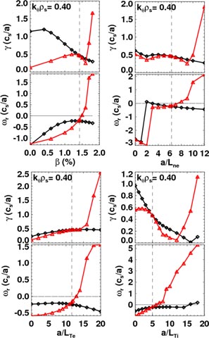
Figure 16. Growth rate and real frequency of the dominant instabilities in the example EP H-mode pedestal, as a function of (upper left) β, (upper right) the density gradient, (lower left) the electron temperature gradient, and (lower right) the ion temperature gradient. See text for additional details.
Download figure:
Standard image High-resolution imageAs the figure shows, if the geometry is held fixed, increasing any one of β, the density gradient, or the electron and ion temperature gradients by less than a factor of two causes a kinetic ballooning mode (KBM) to become destabilized (as evidenced by a sharp increase in the growth rate and a strongly positive real frequency). However, with a consistent MHD equilibrium calculated at each point, KBM onset is never observed. This is consistent with the plasma being in the second-stable regime, which has been verified through calculations of ideal ballooning stability. At the nominal parameters (vertical dashed line), increasing the electron temperature gradient has the strongest destabilizing effect. The density gradient is weakly stabilizing, with microtearing modes appearing at very low values of a/Lne (evidenced by the transition to large magnitude negative real frequency). Increasing the ion temperature gradient is strongly stabilizing, regardless of how the geometry is treated (aside from the transition to KBM). This suggests that the increased ion temperature gradient measured in the EP H-mode does not lead to degraded microstability, and may be consistent with the dominance of neoclassical transport in the ion channel. Overall, the dependences found here are reasonably consistent with the dominant mode being a TEM/KBM hybrid mode as found in pedestal calculations during standard and lithiated H-modes [81] with a smooth transition between negative and positive real frequency as the KBM threshold is approached (in the case where the geometry is held fixed). One difference, however, is the β dependence found here, where increasing β is stabilizing near the nominal value even in the case where the geometry is not changed.
5.3. Comparison of the ion transport to neoclassical theory
As indicated above, both the lack of turbulence changes following the EP H-mode transition and the microstability calculations lead one to question if the EP H-mode Ti profile dynamics are determined by neoclassical physics. In order to make a first test of this hypothesis, the ion temperature profiles for the discharges 134991 (figures 3 and 5), 141340 (figures 2, 5 and 6), and 133841 (figures 5 and 8) have been compared to the results of neoclassical predictions. In particular, the neutral beam heating parameters, electron, ion and impurity density profiles, and electron temperature profiles were used as inputs to the TRANSP code. The ion temperature profile was predicted using the Chang-Hinton model [82] for the neoclassical thermal diffusivities, and no model for anomalous (turbulent) ion heat transport was used.
The results from this analysis are shown in figure 17. The left frame shows the mapped Ti profiles, where the radial coordinate ρpol is defined as the square root of the normalized poloidal flux. The measured profile is shown in blue, while the prediction from the Chang-Hinton model is given in red. The symbols are the values determined by the TRANSP mapping routines. The solid lines are spline fits to these profiles. These spline fits are then used to determine the inverse scale lengths
 shown in the right column, calculated from
 .
.
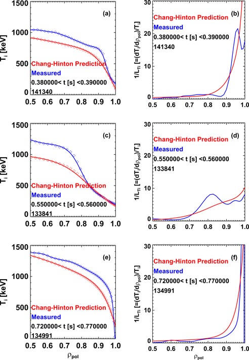
Figure 17. Ion temperature profiles (left column) and inverse Ti gradient scale lengths (right column) during the EP H-mode phase of three discharges. The red curves are from predictions with the Chang-Hinton model, while the blue curves are the measurements as mapped by TRANSP.
Download figure:
Standard image High-resolution imageFor discharge 141340 in the top row, the region of steep Ti is at ρpol ∼ 0.92, and frame (a) shows that the Ti gradient is comparable or exceeds that predicted by neoclassical predictions; this is visible in either the raw profiles, or the higher values of
 in frame (b). Discharge 133841 in the middle row is an example of a case where the region of steep Ti gradient is shifted inwards. In this case, the local gradient clearly exceeds that predicted by this simple neoclassical model. Finally, discharge 134991 in the bottom row has the steep gradient region at the very edge of the plasma. Once again, the Ti gradient appears steeper than predicted by the simple neoclassical model.
It should be noted that this analysis does not indicate that neoclassical theory is violated, as the Chang-Hinton model is a purely local model, based on assumptions that are typically violated in these plasmas. The values of χi have been evaluated with NCLASS [83] and NEO [84] and compared to the predictions from the Chang-Hinton model. They generally show ion thermal diffusivities a factor of 2–3 lower than the Chang–Hinton model in the region of the steep temperature gradient, which would result in a steeper ion temperature gradient. In order to fully understand this physics, these EP H-mode cases are being evaluated with the full-f Monte Carlo code XGC0 [85]. The results of this analysis will be presented in a future publication.
6. Control of the EP H-mode transition
The examples in section 2 show that EP H-modes can be sustained for multiple confinement times in near-stationary conditions. However, to fully exploit this regime, mechanisms to better control the onset and sustainment of the EP H-mode phase must be developed. This section will explore various means of triggering EP H-modes
6.1. Natural onset in low q95 discharges
A first method for routinely generating EP H-mode discharges is to determine a plasma scenario where the plasma naturally transitions to this regime at a reliable and repeatable time. Based on operational experience, it was known that low q95 discharges often had those characteristics, with an early ELM that often triggered a transition to EP H-mode. Hence, this configuration was chosen for a dedicated experiment.
In this experiment, a series of 22 high-current (IP = 1200 kA) discharges were formed; discharge 141340 from figures 2, 5, 6, 16 and 17 was part of this sequence. The first EP H-mode transition occurred in the 3rd discharge, and in 13 of the following 19 discharges. This indicated that, under the right circumstances, these transitions could be fairly reliable. The experimental plan was then to use βN-control [15, 86] to limit the growth of the pressure and avoid the disruption.
A representative discharge from this sequence is shown in figure 18. The discharge transitions to EP H-mode following the ELM at t = 0.34 s, and there is a rapid increase in the stored energy. A region of steep ion temperature also forms, as visible in the t = 0.365 s profiles in figure 18(b), and a local minima in the rotation frequency profile is visible. The neutral beam power is then rapidly ramped down by the βN controller. However, a second ELM at t = 0.380 s causes the plasma to fall out of EP H-mode, and the discharge continues on in traditional H-mode. Note that this and similar H-mode discharges, operating at high current and low power, produced some of the highest absolute confinement times observed in NSTX H-modes, with τE,th ⩾ 80 ms.
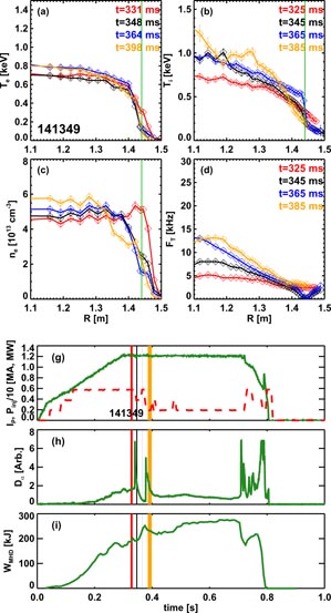
Figure 18. Profile evolution and time traces from a discharge that transitions into and out of EP H-mode. The quantities shown are the same as in figure 6. The plasma is in the EP H-mode state for the middle two times in the profile figures. See text for additional details.
Download figure:
Standard image High-resolution imageHence, while this experiment showed the ability to generate this configuration reliably, it was not possible to maintain the configuration. This underscores the importance of better understanding the macrostability of the edge pedestal [87] in these cases, likely using codes such as ELITE [88, 89] which have proven successful in understanding [53, 60] the suppression of ELMs with lithium PFC conditioning [90] in NSTX. Experimentally, repeating these experiments with heavier lithium conditioning of the PFCs may help delay or eliminate ELMs, if the stability of the EP H-mode pedestal is modified in a way similar to the H-mode modifications [53, 60].
6.2. EP H-mode transitions driven by triggered ELMs
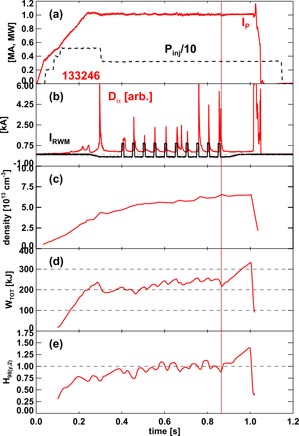
A second means of generating EP H-modes may be to deliberately trigger an ELM, which leads to EP H-mode. ELM triggering has been observed in NSTX via vertical jogs [91] and 3D field application [28–56]. Injection of small pellets has also demonstrated ELM triggering in many tokamaks [92–98]. Figure 19 illustrates a case where a series of pulsed 3D fields are used to generate a sequence of triggered ELMs. This is best illustrated in frame (b) where the small transients in the resistive wall mode (RWM) coil current (black) are each followed by an ELM (the small dc offset in the RWM coil current is for n = 3 error field correction [99], while the applied 3D fields also are n = 3). The final triggering pulse is at t = 0.85 s, and the associated ELM triggers a transition to EP H-mode. The subsequent confinement increase achieves H98(y,2) = 1.3 before the plasma disrupts. Note that this example comes from an experiment designed to study ELM pacing, not EP H-mode transitions. Also recall that the EP H-mode example discussed in figure 8 was initiated by an externally triggered ELM.
Figure 19. Example of EP H-mode configuration initiated by a triggered ELM. Shown are (a) the plasma current and injected power, (b) divertor Dα and RWM coil current, (c) line-averaged density, (d) stored energy, and (e) H98(y,2) confinement multiplier. The vertical line indicates the time of the EP H-mode transition.
Download figure:
Standard image High-resolution image
Motivated by this and other examples, an experiment was done to trigger EP H-mode transitions via pulsed fields. In that experiment, lower current (900 < IP(kA) < 1000) discharges were selected. Lithium conditioning of the PFCs was used, as was super sonic gas injection (SGI), motivated by the use of that fuelling technique for discharge 134991 (see section 2.1). However, despite trying a range of fuelling methods and trigger pulses, it was not possible to generate the EP H-mode configuration via triggered ELMs in this first dedicated experiment. Two discharges from this experiment spontaneously transitioned to EP H-mode before the first externally triggered ELM, and those two discharges are included in the database analysis described above. Hence, while the data like in figure 18 show that it is possible to trigger this configuration with externally triggered ELMs, it is clear that additional characteristics of the discharge play a role. Identifying those characteristics will be a topic of research on NSTX-Upgrade.
7. Summary
This paper has documented many features of the EP H-mode in NSTX. Key findings include:
- While many examples of EP H-modes are short lived, examples exist of longer-pulse EP H-modes of several confinement time duration, including a recently observed very quiescent case (section 2).
- The location of the steep Ti gradient can be either directly at the separatrix, or shifted in a considerable distance. Indeed, the latter cases appear more like discharges with a large-radius internal transport barrier (section 3).
- The largest component of the energy increase following the EP H-mode transition is in the ion channel. Confinement multipliers up to H98(y,2) ∼ 2 have been observed (section 4).
- The EP H-mode regime has been observed over a range of collisionalities and q95 (section 4).
- The steepness of the ion temperature gradient in EP H-mode is correlated with the local gradient in the toroidal rotation frequency shear (section 4).
- No significant changes in the measured fluctuation characteristics in EP H-mode have been observed, compared to similar H-modes (section 5).
- Microstability calculations and neoclassical transport have been initiated. While some microturbulent modes are linearly unstable, the analysis indicates that the ion thermal transport is at or beneath the neoclassical level projected by a simple local model (section 5).
- Experiments designed to reliably form and sustain EP H-mode plasmas have met with mixed success. An experiment to sustain low-q95 EP H-modes was quite successful in generating the configuration, but maintaining the configuration was difficult. While examples exist of externally triggered ELMs resulting in a transition to EP H-mode, a first experiment dedicated to reproducing this effect proved unsuccessful (section 6).
It is interesting to compare this confinement regime to the VH-mode [22–28] observed at JET and DIII-D. VH-mode was first observed with boronization of the DIII-D vacuum chamber [22], though examples without a recent boronization were subsequently observed [26]. The EP H-mode in NSTX was observed before lithium conditioning of the PFCs was common, but the frequency of occurrence has increased with more regular use of lithium as a PFC; the two examples of sustained EP H-modes shown in figure 3 both used Li conditioning of the PFCs. The VH-mode is characterized by edge transport barriers that are broader than in H-mode, which is also somewhat similar to the rather broad edge localized barriers seen in EP H-mode (see figures 7 and 8, for example). However, VH-mode is generally facilitated by the increase in toroidal rotation in the region just inside the pedestal. This is referred to at the 'spin-up' in [26], and this increase in rotation and rotation shear is though to result in a broader region of E × B shear and associated turbulence suppression [26, 27]. In contrast, the EP H-mode is often formed by a localized decrease in toroidal rotation towards the edge, which results in a region of increased rotation shear. Hence, while a region of broad toroidal flow shear may be important for both configurations, the mechanisms by which that flow shear is generated are significantly different. Finally, a key element in achieving high-quality VH-modes was the avoidance of the first ELM following the L-H transition. Reference [26] shows how the experimental actuators that delay the first ELM also result in higher VH-mode performance. In contrast, the EP H-mode is often triggered by an ELM (often the first large ELM following the L- → H transition, as in figures 2 and 6). Hence, while the two regimes share some similarities, there are also many significant differences.
The work presented in this paper represents only an initial assessment of the physics elements of the EP H-mode configuration, with many additional steps yet to be completed.
On the analysis side, it is necessary to better understand numerous physics aspects of these configurations. One key issue is to better understand the peeling–ballooning stability of the configuration. As was indicated in section 6, ELMs during the EP H-mode phase often drive a transition back to H-mode. However, the data in figures 3 and 7 show a case where an ELM occurs during EP H-mode, yet the configuration recovers into EP H-mode again. Due to the large pedestal pressures in these cases, ELMs during EP H-mode would likely be particularly large, with numerous detrimental aspects in a burning plasma configuration. Luckily, examples such as in figures 3 and 7 show long periods in the EP H-mode configuration, without any ELMs. It is likely that the heavy lithium coatings used in these examples assisted in the suppression of these ELMs. A complete assessment of this physics will require numerous peeling–ballooning stability calculations based on kinetic EFITs, a task that has only recently been initiated.
A second key analysis task is to complete a more thorough neoclassical analysis of the ion transport, using the code XGC0, including comparisons to similar H-mode discharges. A single XGC0 analysis of a time slice in discharge 141133 showed that the ion temperature profile could be reproduced using the purely neoclassical transport, but detailed comparisons of the XGC0 results to H-mode examples or simpler neoclassical models have not been executed.
It is also necessary to better understand the microstability characteristics of these discharges. The data in section 5 indicates that turbulent modes are linearly unstable, but that the transport level remains at the neoclassical levels during the EP H-mode phase. Indeed, the observed reduction of the growth rates with increasing Ti gradient may be speculated to provide a bootstrapping effect, where the increased gradient results in reduced turbulent transport. This topic must be revisited with full-physics non-linear turbulence simulations, a challenging task outside the scope of this study.
Experimentally, the key task is to develop better methods to trigger and sustain the EP H-mode configuration.
With regard to triggering, it is necessary to better understand how ELMs trigger a transition to EP H-mode. The data in figure 6 indicate that immediate loss of edge pressure following an ELM leads to a small region of steep gradient Ti, which then increases in width at fixed gradient; a key variable in this case may be the radial width of the zone eroded by the ELM, although systematic studies along these lines have not been attempted. This explanation by itself does not, however, explain the sustained local minima in the rotation profile. As discussed above in section 3.2 and below, there has been speculation that the local minimum is due to torque from a magnetic island at this location, though assessing this physics in detail has proven challenging. This remains a topic of future work.
While spontaneously transitioning EP H-modes appeared repeatable once the discharge scenario was established, further work is required to sustain these scenarios. Heavy lithium conditioning of the PFCs appears to be a plausible means of avoiding ELMs in EP H-mode, provided that it does not prevent the first ELM which drives the EP H-mode transition. If that ELM is suppressed, then externally triggering of the EP H-mode transition appears to be necessary. Further work is required in order to understand the conditions where triggered ELMs actually lead to an EP H-mode transition.
Finally, the potential role of 3D distortions during EP H-mode must be addressed. As can be inferred from the profiles in figure 5, the electron temperature profile is shifted inward compared to the ion temperature profile during the EP H-mode phase. These profiles typically line up well in H-mode, increasing confidence in the spatial calibrations of these diagnostics. However, the diagnostics are toroidally separated by ∼180°, and it is thus possible that the profile shift in EP H-mode is indicative of a 3D distortion. If this were so, the interpretation of the MSE data would also be more complicated and the 2D equilibrium reconstructions used to generate the q-profiles in figures 6–8 would be called into question. On the other hand, the quality of the 2D equilibrium reconstruction, as measured by the goodness of fit parameter χ2, does not degrade following the transition to EP H-mode, and the observed displacements between Te and Ti appear to be independent of the configuration of the known error field sources in NSTX. These latter two considerations appear to imply that the EP H-mode plasma can be understood using 2D axisymmetric equilibria and transport physics, an assumption that has been used for all analysis in this paper.
Overall, this research shows the potential benefits of the EP H-mode configuration for next-step STs, while also illuminating both the transport physics and practical triggering and sustainment uncertainties associated with the configuration. Research to better understand the critical transport physics is ongoing. The experimental aspects of these studies will be continued when NSTX-U [100] commences operation, providing access to regimes with higher field and current, higher hearing power, and lower collisionality [101].
Acknowledgments
This research was funded by the United States Department of Energy (DoE) under contract DE-AC02-09CH11466; it was largely conducted as part of the FY2013 DoE Joint Research Target (JRT) on the physics of high-performance operating regimes without large ELMs. The authors would like to acknowledge helpful discussions with Stan Kaye.
Appendix:: Database of EP H-mode TRANSP runs and equilibrium reconstructions
As part of this study, a database of EP H-mode analysis was created using the codes LRDFIT and TRANSP. A subset of data relevant from this database are shown in table A1. Note that EP H-mode type 0 corresponds to those cases with the steep gradients near the separatrix (diamonds in the scatter plots above), while the type 1 EP H-modes correspond to cases with the Ti gradient shifted inwards (squares in the scatter plots above). The H98(y,2) values are those from figure 10(b). 'eindex' indicates the specific execution of the LRDFIT code used in the database analysis.
Table A1. TRANSP and LRDFIT runs used in this analysis, as well as the times of interest for the various discharges.
| Shot | H-mode time (s) | EP H-mode time (s) | IP (kA) | BT (T) | q95 | H98(y,2) in EP H-mode | EP H-mode type | eindex | TRANSP ID |
|---|---|---|---|---|---|---|---|---|---|
| 129268 | 0.53 | 0.64 | 894 | −0.44 | 9.4 | 1.3 | 0 | −7 | B01 |
| 133246 | 0.865 | 1 | 986 | −0.44 | 7.6 | 1.5 | 0 | −7 | A04 |
| 133841 | 0.43 | 0.56 | 794 | −0.44 | 10.2 | 1.2 | 1 | −9 | B09 |
| 133851 | 0.42 | 0.526 | 794 | −0.44 | 10.3 | 1.1 | 1 | −9 | B06 |
| 134970 | 0.25 | 0.27 | 894 | −0.47 | 9.3 | 1.1 | 1 | −9 | B06 |
| 134987 | 0.89 | 0.98 | 871 | −0.47 | 9.2 | 1.6 | 0 | −7 | B04 |
| 134991 | 0.5 | 0.725 | 888 | −0.47 | 9.6 | 2.0 | 0 | −4 | A22 |
| 135192 | 0.5 | 0.69 | 795 | −0.44 | 10.2 | 1.0 | 1 | −7 | B01 |
| 138169 | 0.25 | 0.32 | 910 | −0.44 | 9.6 | 1.0 | 0 | −4 | A02 |
| 138173 | 0.23 | 0.32 | 968 | −0.44 | 8.6 | 1.0 | 0 | −4 | A02 |
| 138216 | 0.31 | 0.36 | 1205 | −0.44 | 6.4 | 1.0 | 0 | −12 | A28 |
| 138217 | 0.34 | 0.37 | 1212 | −0.44 | 6.7 | 0.8 | 0 | −10 | A06 |
| 138219 | 0.33 | 0.36 | 1202 | −0.44 | 6.5 | 1.1 | 0 | −10 | A21 |
| 138222 | 0.31 | 0.35 | 1217 | −0.44 | 6.6 | 0.8 | 0 | −10 | A17 |
| 138226 | 0.28 | 0.32 | 1141 | −0.44 | 6.5 | 0.7 | 0 | −10 | A14 |
| 138522 | 0.25 | 0.3 | 1056 | −0.44 | 6.1 | 0.7 | 0 | −10 | A05 |
| 138524 | 0.255 | 0.28 | 1063 | −0.44 | 6.0 | 0.7 | 0 | −10 | A04 |
| 138532 | 0.315 | 0.33 | 1271 | −0.44 | 5.9 | 0.6 | 0 | −10 | A02 |
| 138540 | 0.3 | 0.328 | 1212 | −0.45 | 6.3 | 0.6 | 0 | −10 | A03 |
| 139016 | 0.3 | 0.335 | 701 | −0.49 | 11.2 | 1.3 | 0 | −10 | A09 |
| 139281 | 0.3 | 0.335 | 1205 | −0.39 | 5.6 | 0.8 | 0 | −10 | A09 |
| 139349 | 0.4 | 0.55 | 1009 | −0.44 | 7.9 | 0.9 | 1 | −9 | B05 |
| 139605 | 0.23 | 0.266 | 885 | −0.47 | 11.5 | 1.3 | 0 | −12 | A07 |
| 139771 | 0.24 | 0.275 | 903 | −0.47 | 8.9 | 1.2 | 0 | −9 | A06 |
| 139905 | 0.715 | 0.795 | 887 | −0.47 | 7.4 | 1.4 | 1 | −12 | A05 |
| 139913 | 0.445 | 0.515 | 862 | −0.47 | 8.1 | 1.3 | 1 | −12 | A02 |
| 139958 | 0.63 | 0.72 | 904 | −0.44 | 8.9 | 1.5 | 0 | −12 | A06 |
| 140108 | 0.38 | 0.4 | 1105 | −0.49 | 8.4 | 0.8 | 0 | −12 | B06 |
| 140161 | 0.38 | 0.48 | 806 | −0.44 | 10.2 | 1.3 | 1 | −9 | B03 |
| 141133 | 0.65 | 0.85 | 896 | −0.44 | 9.1 | 1.5 | 0 | −7 | B11 |
| 141146 | 0.675 | 0.84 | 991 | −0.44 | 8.1 | 1.2 | 0 | −12 | B02 |
| 141177 | 0.49 | 0.555 | 891 | −0.44 | 10.2 | 1.2 | 0 | −7 | B04 |
| 141186 | 0.92 | 0.98 | 901 | −0.44 | 9.1 | 1.4 | 0 | −9 | B04 |
| 141187 | 0.35 | 0.585 | 903 | −0.44 | 10.0 | 1.3 | 0 | −12 | B08 |
| 141337 | 0.34 | 0.385 | 1209 | −0.44 | 6.2 | 0.9 | 0 | −12 | B18 |
| 141338 | 0.31 | 0.35 | 1201 | −0.44 | 6.5 | 0.7 | 0 | −12 | B09 |
| 141339 | 0.3 | 0.375 | 1208 | −0.44 | 6.4 | 0.7 | 0 | −12 | B05 |
| 141340 | 0.32 | 0.39 | 1215 | −0.44 | 6.2 | 0.8 | 0 | −12 | B04 |
| 141343 | 0.34 | 0.365 | 1207 | −0.44 | 6.3 | 0.8 | 0 | −12 | B04 |
| 141344 | 0.31 | 0.35 | 1206 | −0.44 | 6.5 | 0.7 | 0 | −12 | B07 |
| 141345 | 0.305 | 0.365 | 1208 | −0.44 | 6.4 | 0.7 | 0 | −12 | B09 |
| 141346 | 0.33 | 0.375 | 1213 | −0.44 | 6.2 | 1.0 | 0 | −7 | B17 |
| 141347 | 0.335 | 0.365 | 1211 | −0.44 | 6.3 | 0.7 | 0 | −12 | B05 |
| 141348 | 0.31 | 0.35 | 1207 | −0.44 | 6.5 | 0.7 | 0 | −12 | B06 |
| 141349 | 0.34 | 0.375 | 1210 | −0.44 | 6.3 | 0.7 | 1 | −12 | B05 |
| 141353 | 0.34 | 0.366 | 1201 | −0.44 | 6.6 | 0.8 | 0 | −12 | B13 |
| 141354 | 0.34 | 0.375 | 1203 | −0.44 | 6.6 | 0.9 | 0 | −12 | B03 |
| 141454 | 0.25 | 0.33 | 894 | −0.44 | 10.5 | 1.1 | 0 | −7 | B05 |
| 141476 | 0.38 | 0.58 | 818 | −0.44 | 11.3 | 0.9 | 0 | −9 | B06 |
| 141761 | 0.2 | 0.265 | 846 | −0.54 | 10.4 | 0.7 | 0 | −9 | B04 |
| 141768 | 0.2 | 0.32 | 846 | −0.54 | 9.6 | 0.9 | 0 | −9 | B04 |
| 142185 | 0.2 | 0.28 | 925 | −0.54 | 10.0 | 1.0 | 0 | −9 | B06 |