
Abstract
Quantum optics and classical optics are linked in ways that are becoming apparent as a result of numerous recent detailed examinations of the relationships that elementary notions of optics have with each other. These elementary notions include interference, polarization, coherence, complementarity and entanglement. All of them are present in both quantum and classical optics. They have historic origins, and at least partly for this reason not all of them have quantitative definitions that are universally accepted. This makes further investigation into their engagement in optics very desirable. We pay particular attention to effects that arise from the mere co-existence of separately identifiable and readily available vector spaces. Exploitation of these vector-space relationships are shown to have unfamiliar theoretical implications and new options for observation. It is our goal to bring emerging quantum–classical links into wider view and to indicate directions in which forthcoming and future work will promote discussion and lead to unified understanding.
Export citation and abstract BibTeX RIS
Introduction
Familiar concepts serve to link quantum optics and classical optics in ways that are only now beginning to be investigated. We are referring to elementary notions of optics, whether quantum or classical, such as interference, polarization, coherence, and entanglement. To begin, we consider polarization. In ordinary language polarization refers to concentration around a given value or within a given realm, as one understands a polarized electorate to mean a concentrated orientation of voters' views in one or another direction. The term in optics will become more usefully descriptive when liberated from specific reference to the spin degree of freedom of light. For this reason we will speak of spin instead of polarization, and use the word polarization as a generic technical term and not specifically associated with spin.
With respect to coherence one can say almost the same thing. In ordinary language coherence can mean practically anything, and unfortunately this is also true in physics and optics. The fact is that coherence has never been defined quantitatively. This means that there is no accepted value scale associated with coherence, a scale that could be consulted in order to say that in context A there is twice as much coherence as in context B, and not run the risk of confusing the meaning of coherence for context C. We accept also that coherence is somehow necessary to achieve or exhibit interference, whether visibility is available to measure every kind of interference or not.
Entanglement
The beginning remarks above leave entanglement still to be examined among the elementary notions mentioned. It is more difficult to deal with, although well defined and having accepted scale measures, because of its unnecessary association with quantum theory. This is Einstein's fault [1], because Schrödinger [2], in his well-known reply to Einstein in 1935, was forced to deal with the red herring of locality in the same way that Einstein framed it, as a statement of positional location. To an abstract quantum state, positional location has no relevance, although it may play a critical role in experimental operation. Quantum states have only statistical and probabilistic significance, and the term non-local only means that two parties are statistically distinct and independent of each other. Such a statistical independence can sometimes be experimentally guaranteed for two parties by their remote relative location, but this requires careful preparation, and the amount or distance of remoteness has nothing to do with the degree of statistical non-locality. In any event, the definition of entanglement is simply inseparability of sums of product states that exist in different vector spaces. Schrödinger indicated this explicitly [2] as non-factorization in a joint function space:  , while calling attention to a much earlier paper by Erhard Schmidt for the mathematical theorem [3] that applies in all Hilbert spaces, theoretically abstract or experimentally concrete. To emphasize this, we should keep in mind that entanglement is a vector space property, present in any theory with a vector-space framework. Thus there is no distinction between quantum and classical entanglements, as such. The important differences between the quantum and classical theories of light do allow quantum entanglements to be exhibited in a wider variety of ways, but of course these are never observed unless detection capability makes individual photons experimentally distinguishable.
Electric field states in optics
Optics refers to experimental realizations and consequences of the behavior of electric fields in the visible part of the electromagnetic spectrum. When we think of optical coherence and interference we typically have nearly monochromatic behavior with a specific direction of beam propagation in mind, which we will take as the z direction. After removing a z- and t- dependent propagation factor we can write the associated transverse complex electric field at an unspecified location as

where  and
and  are spin unit vectors in the x and y directions, and the components are to be understood as the positive-frequency or analytic-signal amplitudes of the real (Hermitian) electric field. The term 'partial polarization' in optics refers to an indefinite overall spin direction, which operationally means that it is impossible to find a unit vector direction
  that allows the field to be written
  . That is, no single spin orientation
  is able to capture all of the light. This means that two spin vectors and two amplitudes are needed to describe the field, and their inseparability in (1) expresses entanglement of those two degrees of freedom of the field. Thus entanglement is present in all instances of what is conventionally called partially polarized optics, whether treated classically or quantum mechanically. Since it is impossible to assert with 100% confidence that any optical field is absolutely perfectly polarized in the ordinary sense (i.e., uniquely spin-oriented), we will continue attention to indefinite (or partial) spin orientation, and will naturally have to examine the consequences of the associated entanglement [4–8].
Several polarizations and degrees of freedom in pairs
Quantification of a degree of spin concentration is obviously possible because it's the same as finding the degree of conventional light polarization. A high degree means that the component amplitudes Ex and Ey are such that there is a spin direction, say  , in the neighborhood of which not all but most of the total amplitude is concentrated. In the 1850s Sir George Stokes first indicated [9] how to determine the degree of such concentration, conventionally written
  . The pioneering studies of Emil Wolf a century later in the 1950s [10–12] showed how
  is determined by the amount of correlation existing between the amplitudes:

through the determinant and trace of  , the spin-polarization coherence matrix [13, 14], which is given by
where the suffix s indicates that spin polarization is intended. The quantum and classical equivalents are obvious: ![$\langle {E}_{i}^{*}(t){E}_{j}(t)\rangle \leftrightarrow {\rm{Tr}}[\rho (t){E}_{i}^{(-)}{E}_{j}^{(+)}]$](https://content.cld.iop.org/journals/1402-4896/91/6/063003/revision1/psaa2205ieqn11.gif) .
.
In the general case a light field is independently a function of x, y, z, t, and spin orientation. Each of these degrees of freedom identifies a vector space, an independent sector of what is obviously a multi-sector space (see [15] for an overview). Many options are open to be specified experimentally. For example, a light beam with its spin component fixed along  could be a superposition of two different temporal functions, each with its own space function. This is a three-sector description of
  . The field would again be entangled, but now entangled between the temporal and transverse positional degrees of freedom. A specific example is indicated in the expression here for A in
  :
:

In this case the question of polarization in a generic sense, arises not for spin, because that is fully concentrated, pinned down in the spin sector to the direction  , but it remains an open question for the time t and transverse spatial location
  sectors, which cannot be factored apart in
  .
.
Still, the degree-of-polarization procedure for (4) is exactly the same as for the field in (1). Suppose the two spatial functions  and
and  are experimentally chosen to be two different modes that are orthogonal across the beam. Then they play the same basis-vector role as the
  and
and  unit vectors in (1), and we could abbreviate
  and
and  for simplicity by
  and
and  , with
  . For
. For  in (4) the coherence matrix in the two-dimensional spatial-mode sector with basis
  , is then given by

where  is the ij element [16] of
  and the r subscript signals that polarization of the spatial degree of freedom is at issue. The result is the reduced matrix obtained from the dyadic tensor
  by tracing over the t sector, via the complete set of modes in which the F functions can be expanded.
For pure states such as (4) this could be done in the other order, by tracing over the spatial modes, leading to a different reduced matrix  . These paired coherence matrices provide the same degree of polarization:
  , which follows from the basic definition

Explicit calculations of both  and
and  have been provided for comparison by Qian and Eberly [7].
The first experimental work directed at a polarization in the complete absence of conventional (spin) polarization has recently been undertaken, and the analog of the usual Poincaré sphere has been mapped in detail [17] (see figure 1). This new form of polarization not associated with spin can be present in a classical as well as a quantum description of the field in (4). To emphasize this, the experiments were made completely classically. Each spatial function used to define  in the experiments was a low order Hermite-Gauss laser mode, and the temporal functions were stochastically uncorrelated, obtained from a laser diode running below threshold and providing classical (thermal) statistics. Detection was also classical, made with a power meter, not by photon counting.

Figure 1. Experimental data (see [17]) showing polarization of transverse mode states on the plane  of the analog Poincaré sphere, highlighting the linearly polarized states.
Download figure:
Standard image High-resolution imagePairwise polarization and entanglement
The  fields in (1) and (4) exhibit entanglement of two degrees of freedom, time and spin in the first case, and time and space in the second. The values of the degree of the paired entanglement in each case are easily obtained if the fields are rewritten in Dirac notation. Each degree of freedom defines its own vector space, and the two fields in (1) and (4) can then be written (the tensor product symbol ⨂ is hardly necessary):


The use of boldface is only a reminder that the boldface state contains more than one vector space (degree of freedom). In  the
the  and the sine and cosine functions are inserted to allow the
  and
and  states to be unit-normalized,
  , while signaling that the intensities associated with the two components are fixed at
  and
and  .
.
The use of Dirac notation prompts the recognition that the classical optical fields (7) and (8) are mathematically the same as states in quantum theory, in fact pure states. This raises an unusual question in optical coherence theory—what is the expression for an optical field that is not a pure state field? In experimental practice ideally pure quantum states are non-existent, and the same is true of optical fields, so the question of classically mixed optical states should be addressed. This is done in a later section, and for the time being we will assume that the fields to be discussed are sufficiently ideal that we can treat them as pure.
Conveniently, we can experimentally choose the spatial states  in
in  to be orthogonal,
  , but the time-dependent
  states are generally not orthogonal, so we introduce the state
  , the orthogonal partner [18] of
  , and write

where obviously  . Then we write
  , the unit-normalized version of
  , in terms of the 4 orthogonal and normalized basis state pairs:
Clearly, only a term proportional to the two-party basis state  is missing, compared to a general two-party GF state
The concurrence of Wootters [19] evaluates the degree of entanglement of the time-space  as
as  , in the standard range
  , and the degree of entanglement in the unit-normalized field (10) is found the same way. We simply read off the coefficients in (10) to obtain the value of the entanglement between the F and G, or time and space, degrees of freedom:

To compare to this degree of entanglement, we ask what can be said about the degree of polarization in the same tr sector of the vector space? We can use (6) with the replacements made above:  and
and  to obtain
By referring to (12) we see that this result yields a new relationship:

where  is either
  or
or  . This has recently been discussed [17] as an analog of complementarity.
Finally, a two-sided reminder: the Dirac notation is only notation, and does not make any of the classical quantities (even the entangled ones) quantum mechanical. On the other hand, because of the implicit association of amplitudes with positive-frequency fields (analytic signals), essentially all of the fields and functions can be considered quantum mechanical fields/states if desired, for the purpose of the low-order correlations that will be under consideration. At the same time, this reminder prompts a question addressed in the following section.
Where is the optical quantum-classical border?
What is known as 'Bell violation' is commonly accepted as the signal of purely quantum behavior, and thereby a marker of the quantum–classical border. The background for this is well known. In 1964–1966 John Bell presented [20] a specific logical inequality that can be contextually interpreted, and in different forms it has been tested experimentally (see [21–25]). A limit on the value of a physically accessible correlation measure is predicted by the inequality, but the limit can be violated under photonic examination. This is in agreement with quantum theory, which predicts that the limit can be exceeded. Thus a violation is commonly accepted as evidence of the quantum character of the demonstration.
However, a crack in the foundation of this conclusion is one consequence of a remark of Bell himself [26] in 1972: 'It can indeed be shown that the quantum mechanical correlations cannot be reproduced by a hidden variables theory even if one allows a 'local' sort of indeterminism. .... This would not work.' This turns out to be the weak point in the common acceptance mentioned above because recent reports using classical light show the contrary—it does work. It works under two conditions: (a) if one stays within a limited but well-studied domain of classical wave physics, a domain where postulated non-determinism provides theoretical predictions that agree with experimental observation, and (b) if entanglement is available.
As Shimony has said (see p 30 in [27]), '[Bell] asks ... whether a contextual hidden variables theory ... is able to recover the statistical predictions of quantum mechanics without introducing physically undesirable features'. In order to be serious, a theory needs to embrace in some way those aspects of Nature that appear completely random, i.e., purely statistical, and that are dealt with by quantum theory in well known ways. This is the reason for Bell to raise the issue of classical indeterminism. Shimony summarized this by naming three key features, all of which would have to be part of any fundamentally interesting physical theory:
- I.In any state of a physical system S there are some eventualities which have indefinite truth values.
- II.If an operation is performed which forces an eventuality with indefinite truth value to achieve definiteness ... the outcome is a matter of chance.
- III.There are 'entangled systems' (in Schrödinger's phrase) which have the property that they constitute a composite system in a pure state, while neither of them separately is in a pure state.
By eventualities Shimony meant measurement outcomes.
Recent experiments [28–36] conforming to criterion III (viz., employing classically entangled light fields) show that the Clauser-Horne-Shimony-Holt (CHSH) [37] form of Bell's inequality can be strongly violated without invoking quantum mechanics at all. Relatively few tests have embraced criteria I and II as well as III. The probabilistic indeterminism that I and II call for is intrinsic to 'natural' light, i.e., spin-unpolarized and statistically thermal. Figure 2 shows the results of one test [38] conforming to all three criteria, to demonstrate the extent to which violation can be obtained. This eliminates Bell violation as a universal quantum–classical boundary marker.
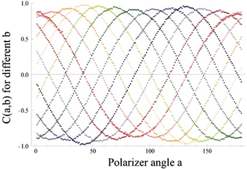
Figure 2. Plots of the CHSH correlation function  obtained by scanning polarization angle a and holding angle b constant. The invariant cosine function required to violate the Bell inequality is clearly present. Values for the Bell parameter were obtained in the range
  , many experimental standard deviations beyond the Bell violation limit
  . See arXiv:1307.3772, arXiv:1406.3338 and [38].
Download figure:
Standard image High-resolution imagePartially coherent states that are not mixed
At this point in our treatment of multi-sided quantum–classical connections, we can deal with a confusion in wording. It is sometimes said (see, e.g., Svozilik et al [39]) that any partially coherent state is a mixed state, but this needs to be carefully understood because it is not strictly correct. We return to the matrix  in (3). The matrix represents a state that is at best partially coherent in the sense of spin orientation. That is, thinking of the standard expression of the degree of polarization (2), the condition det
  is not met. However, the field (1) that it represents is not mixed; it is clearly a two-party pure state—a bilinear combination of products of vectors in two distinct vector spaces (but not quantized). This highlights a frequent objection directed at either the arithmetic or the notation: how can a pure-state description be possible for a field that is only partially coherent, not completely polarized?
But there is no contradiction, and a familiar quantum analog can present the same situation. Consider the quantum state for an atomic electron in a superposition of positional and spin states:

This state is certainly a pure state, but its degree of spin polarization can easily be checked to be less than 1. This is the case whenever  and
and  do not satisfy
  . Thus, we would label the electron's state as only partially spin-coherent, even though it is a pure state. The equivalent situation in the optical field case is that generally
  , despite the fact that
  is a pure field state.
Coherence hiding: intrinsic and by design
Here we must pay attention to the number of vector space sectors that are available. We have noted elsewhere [15] that the theory of optical coherence was originally based on a restricted form of correlation, in which only one sector in a multi-sector vector space is engaged. The simplest example is autocorrelation within a single sector, as can be arranged by studies of the time sector with a Michelson interferometer. Observations of output intensity yield such averaged quantities as the temporal autocorrelation  , where V is a generic scalar optical 'signal'. The field is either well correlated with itself or not, and there is nothing else to be learned.
The introduction of a vector degree of coherence, to supplant the original scalar theory, was an incomplete first step toward control of the multi-sector character of coherence (see Karczewski [40]). A two-sector example is provided by the field in (1) itself, and its coherence properties are exposed by the matrix  in (3) and the degree of polarization
  . In that case each pair of values accessible in one of the vector spaces, e.g., each of the four
  pairs, brings a companion
  pair into view. The coherences exhibited are strictly pairwise here. The two independent degrees of freedom of the light field (amplitude and spin) are polarized (concentrated) at the same time, not independently, in expression (1). This means that additional coherence can't be found by examining the 'amplitude correlation' matrix
  in addition to the 'spin correlation' matrix
  . The second st coherence measure is easily worked out (see equations (7) and (9) in [7]), but the 'amplitude correlation' matrix conveys no more information than the 'spin correlation' matrix. The correlation obviously belongs to the pair together.
However, our tr examination in the earlier section opened a window on the three-sector case (see historical overview in [15]). Although working with a fixed spin as in (4), by allowing the t and r spaces to remain open for study we can say that all three t and r and s sectors are in principle active. If spin were not fixed at a single value, all pairwise forms of polarization would be available: ts and tr and sr. What we saw in the limited example is itself interesting. We saw that an experimenter can in effect 'hide' both sr and st coherences, i.e., make them unavailable for detection, by accepting only the part of the field proportional to  . This example alerts us to an important exception to what seems to be a pairwise rule of thumb as described above. Fixing spin on a single value, say on sy, totally 'concentrates' it without sharing with a partner.
This comment can be pursued, as follows. Instead of selecting a degree of freedom (by a projection process), and thereby removing it from further consideration, an experimenter can arrange to simply ignore it. This also removes it from consideration, but the 'hiding' is different. This second type of discarding accepts indiscriminately all values possible for the to-be-discarded degree of freedom, and thus misses its effects. In the case of three sectors, this usually means that the remaining two-sector state will be mixed.
To examine this situation, which is beginning to receive attention [8, 15, 34, 39, 41], we consider the same field as in (4), but complete it as a z-propagating beam field by adding an sx transverse component:

To simplify our task we again allow both the temporal and transverse spatial elements of the field to be represented by just two functions each, and we will insert separately the same sine and cosine factors used earlier to indicate relative intensity differences, and now we will have  because of the two spin components. In this special example the x and y amplitudes can be written:
Now we address experimental disregard. Accepting indiscriminately all of the spin contributions to the field means summing the two contributions that can be observed, namely  , i.e., the trace of the dyadic
  over the spin space. The result is a field state, generally mixed, with contributions from both t and r sectors. A first objective is to find the coherence matrix equivalent to the
  obtained in (5) for a pure state. We write the contributions from the individual sx and sy projections as the reduced matrices in the orthonormal
  representation:

where c and s stand for cosine and sine of  , and
, and

The total trace is the sum of these two matrices:  , where
  is the coherence matrix after both s and t sectors have been traced out:
Several interesting points emerge. Note that γ is the indicator of incoherence at the level where only one spin component is active, i.e., in each of (18) and in (19). We can label it as 'intrinsic' incoherence in the sense that γ comes from a feature of the field itself:  . Thus we see that if we simply remove it by taking
  , we find both (18) and (19) to be pure-state matrices, representing fully coherent states.
Notice however, that even after we remove the 'intrinsic' incoherence by taking  , the final total coherence matrix (20) remains mixed. This impurity arises from incoherence that was introduced by the failure to make precise enough observation, i.e., by failing to segregate the two spin components for individual study. It might be called observational incoherence. Finally, note that if
  and
and  , then even the observational incoherence disappears. This is because the condition
  means that
  , so F1 and F2 have equal intensities, and then there is no possible distinction between
  and
and  anyway, so combining them indiscriminately in the observation has no negative consequences.
Extended field entanglement
None of the three trs degrees of freedom contained in the version of  in (16) can be factored apart. In this case the question of polarization in the wide sense arises for all three labels together, t and r and s. The combination of three classical degrees of freedom leads to consequences that have direct quantum analogs, and vice versa. See [42] for the formulation of new constraints on three-qubit quantum states. Classical optical physics may provide an ideal ground for realization of new forms of generalized polarization [43], and it has already permitted experimental realization of entangled mode swapping [44], a recognizable version of teleportation if vector-space de-localization is substituted for laboratory de-localization.
One can see that the optical field (16), made specific in (17), can be interpreted as a three-qubit pure state. We can even expand the description to write the optical field as a (non-quantum) state of N qubits, a superposition of  terms:

where  are normalized coefficients and sj indicates a generalized spin, taking value 0 or 1 corresponding to the two states
  ,
,  of the j-th qubit, with
  . The other classical 'qubits' represent additional two-state degrees of freedom, extensions of the
  and
and  states employed already.
The Schmidt theorem [3] provides a powerful restriction on such tensor products of two-valued states, which have obvious quantum analogs of wide interest. It permits a generalization of the approach already sketched in obtaining the matrix  . In retrospect it was the result of bi-partitioning the field
  by treating the sx component of the spin degree of freedom independently of the sy component, which was temporarily ignored, and separately from the two t and r degrees, which retained mutual coherence. We could alternatively have joined the t and r degrees of freedom into a new 'larger' degree of freedom with four values, 00, 01, 10, 11, while the s degree of freedom remains effectively a qubit with only two values, 0 and 1. For the N-qubit state a similar separate identification of one degree of freedom creates a larger 'leftover' state where all N-1 other degrees of freedom are considered as a single second party (similar to the t and r pair taken together).
Two-term entanglement
Having only two non-zero eigenvalues, the effect of the Schmidt theorem is that the entire state itself behaves like a qubit. Thus the optical field (21), no matter how many degrees of freedom are identified for it, can be reduced (after separating the jth qubit from the rest) to a sum of only 2 rather than  terms:

where  and
and  are the 'information eigenstates' of the reduced density matrices of the j-th qubit and the remaining
  qubits, from whose joint state the Schmidt theorem [3] determines the unique two-dimensional partner of the jth qubit. One must keep in mind that our vector-state analysis applies to quantum as well as classical states, and a multi-photon quantum state can have many more degrees of freedom to work with than the classical fields we are examining.
The two Schmidt numbers  are the corresponding eigenvalues of the reduced density matrix for one party, i.e., the jth qubit, and are the same for both parties, and satisfy
  . The degree of entanglement between the j-th qubit and the remaining
  qubits can be characterized in a number of ways, frequently by the Schmidt weight Kj, which is defined in [45]:
  . For our purposes an alternate normalized form, also serving as an entanglement monotone, is more useful:

Here  is less than or equal to
  and Yj obviously satisfies
  , where 0 indicates complete separability (zero entanglement), and 1 denotes maximal entanglement.
The key result for the Yj entanglement measure is the proof [42] of an entanglement-dilution inequality. It applies to all the Yj values for the N qubits:

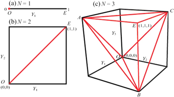
The N different Yj entanglements identify axes in a unit N-dimensional space. All possible N-dimensional vectors  live inside a unit N-dimensional hypercube, since
  . The cube's origin
  represents zero entanglement, corresponding to completely separable states, while the opposite corner
  represents maximal entanglement. It is worth stressing that
  is invariant to unitary local transformations of the state. The new inequality (24) implies that the region inhabitable by the vectors
  (for pure states) is not only just inside the N-dimensional unit hypercube, but concentrated within the two pyramids that share the triangle ABC as their base planes.
Versions of this 'cube' are shown for N = 1, 2, 3 in figure 3. The concentration that this implies ensures that entanglement must be shared. This can be seen directly by adding another Yj to the left side of (24). The right side becomes the total of all the entanglements, and the inequality now mandates that the jth degree of freedom can contain no more than half of the total. The remaining entanglement must be shared among j's N-1 partners.
Figure 3. The first three N-dimensional spaces in which the vector  is defined. The entanglement sharing 'volume' is clearly zero until N = 3 when the entanglement vector
  must fall within the two pyramids having apex points O and E, and sharing the triangle ABC as base plane (see [42]. Reproduced with permission. Copyright The Optical Society 2015.).
Download figure:
Standard image High-resolution image
Mixed electric field states
We can make use of results based on the entanglement measure  in talking about optical fields. They apply immediately to a field such as the example discussed in the preceding section. We will confine attention here to N = 3, which restricts the three Y values to form a vector
  lying inside the pyramids that are inside the cube in figure 3. We can think of a version of the three-sector field given in (16) in the framework of the state (21), where spin, time and space mode sectors are represented by states with two orthogonal orientations, while allowing for an arbitrary set of coefficients. For example, such a division of the field among the sectors could be:


where  . We can identify the three spaces in (26) with str, the spin, time and space sectors of an optical field's vector spaces, as in (25), but more generally simply regard them as signifying different pairs of orthogonal modes or two-valued degrees of freedom of the state, without attempting to continue their connection to a specific field. In this way they are free even to belong to pairs or groups of individual photons that happen to be entangled, allowing a range of non-classical qubit interpretations.
We can obtain specific examples of mixed states if we impose 'disregard' conditions appropriately. Instead of projection, we trace out each of the three vector spaces in turn, the three reduced coherence matrices, representing the optical field via the (still observable) remaining two parties, are given as follows:
and
The label outside the vertical bar indicates a space or spaces traced over, and the letters inside the bar indicate the spaces remaining after the tracing. The partial symmetry is easily explained. The first two sectors, s and t, take the same value in each term of (26). By projection on either  or
or  of those two sectors, the remaining state is separable. This is not true of projection on either
  or
or  of the r sector. The equality in (28) only means that the form is the same for the 4 × 4 matrices remaining after the trace, although the four-dimensional state spaces
  and
and  in which the matrices are displayed are obviously not the same.
Generic polarization and extended entanglement
The most striking consequence of the introduction of the  measure is its relation to field polarization, which is even simpler than the relation of
  to concurrence that we encountered earlier. The connection between the Schmidt eigenvalues and polarization is known in various forms (e.g., see Qian and Eberly [7] and, without trace normalization, in Wolf, chapter 8 [14]). Its relation to Y is simply expressed in our notation for any degree of freedom, i.e., any j, as

The three different Y values are easily calculated, leading to these polarization values for the field in (26):
which indicate that the pure-state pairwise polarization concept needs modification [43] in the mixed-state domain. By converting from  to Y, one can check that the fundamental inequality (24) recently discovered [42] is satisfied three times, as required. We note that all polarizations are equal in the fully symmetric case, such that
  .
.
As a final note we can specialize (25) to make a connection to our introductory remarks. Let us retain  , but allow
  for field (25). Then we project it on
  in order to fix the 'unspecified location' mentioned for expression (1). Thus we can identify
  and
and  as well as
  and
and  , so
, so  corresponds to the present
  . Another trace, to reach the appropriate 2 × 2 subspace, then provides the standard coherence matrix given first in (3).
Summary
Whether quantum or classical, optics has elementary notions such as interference, polarization, coherence, and entanglement that can be considered universal. Our focus here has been to highlight the importance of recognizing that an elementary feature, commonly overlooked altogether, is also universal. This is the participation of several degrees of freedom in almost every imaginable optical situation. The myriad relationships possible among the participating degrees of freedom is the foundation of optical versatility.
We have not attemped to address the complete realization, i.e., observation/detection, of field states with more than two independently active degrees of freedom. The beam coherence polarization matrix (see Gori et al [46]) can be mentioned as an early version of 4 × 4 representations of an optical field, very general forerunners of our fields (27) and (28), but directed to a specific elementary optical apparatus, the Young interferometer. Implementation of vector-space control directed at challenges in polarimetry have been mentioned and a number of proposed innovations based on non-separability and directed at different aspects of optical fields have raised issues of non-traditional polarizations and coherences (see Kagalwala et al [34], De Zela [8], Svozilik et al [39], Balthazar et al [41], and Qian et al [17]), including discussion of the connection to complementarity (see Lahiri et al [47]), indicating the increasing attention being devoted to this complicated topic.
We have pointed to ways in which entanglement, i.e., state non-separability, is at the heart of understanding coherence more deeply. Creative investigations more than two decades ago began the process of engaging the power of entanglement in classical studies, usually without mentioning entanglement and without field quantization, but exploiting the power of the Schmidt theorem through the version due to Mercer (see Fedorov and Miklin in [3]). Pioneering initiatives in the 'pre-entanglement' era by the groups associated with Emil Wolf and Franco Gori must be particularly mentioned. The first recognition that classical optical fields could exploit entanglement in a natural way and thereby engage questions that were considered at the time to be intrinsically quantum mechanical is attributed to Spreeuw. He showed theoretically [4] that violation of a Bell Inequality should be accessible to classical optical experiments, and a number of experimental works that followed were noted [28–36].
Despite several detailed examinations of the multi-sector relationships between coherence, polarization, and entanglement (see Kagalwala et al [34], De Zela [8] and Eberly [15]) a widely accepted and quantitative meaning for the word coherence is still lacking. Our examples advance the proposition that deeper understanding will be further promoted by exploiting the connection between entanglement and a generic understanding of polarization. This may be particularly valuable insofar as it expands polarization's quantitative character beyond the pairwise domain that it has traditionally occupied. It will be helpful to recognize polarization as an attribute independent of the spin degree of freedom, and our examples have focused on multiple types of polarization and ways they can be either 'concentrated' or 'hidden'.
Acknowledgments
We are pleased to acknowledge financial support for visiting scholars provided by CONACyT of Mexico, the Natural Sciences and Engineering Research Council of Canada and the Higher Education Commission of Pakistan. We thank hosts for recent opportunities to discuss the results presented here, in the Center for Nonlinear Science, Los Alamos National Laboratory; Institut für Quantenphysik, Universität Ulm; 5. Physikalisches Institut, Universität Stuttgart; Centre for Quantum Technologies, National University of Singapore; Texas A & M University Institute for Quantum Science and Engineering; Beijing Computational Science Research Center; Department of Physics, Ohio State University and Laboratory for Laser Energetics, University of Rochester. We also acknowledge partial financial support provided by: University of Rochester Research Award; ARO W911NF-14-1-063NSF; DARPA W31P4Q-12-1-0015; NSF Grants PHY-1203931, PHY-1505189, INSPIRE PHY-1539859; and ONR NO: N00014-14-1-0260.