


ABSTRACT
We present the temperature and polarization angular power spectra of the cosmic microwave background derived from the first five years of Wilkinson Microwave Anisotropy Probe data. The five-year temperature spectrum is cosmic variance limited up to multipole ℓ = 530, and individual ℓ-modes have signal-to-noise ratio S/N >1 for ℓ < 920. The best-fitting six-parameter ΛCDM model has a reduced χ2 for ℓ = 33–1000 of χ2/ν = 1.06, with a probability to exceed of 9.3%. There is now significantly improved data near the third peak which leads to improved cosmological constraints. The temperature-polarization correlation is seen with high significance. After accounting for foreground emission, the low-ℓ reionization feature in the EE power spectrum is preferred by Δχ2 = 19.6 for optical depth τ = 0.089 by the EE data alone, and is now largely cosmic variance limited for ℓ = 2–6. There is no evidence for cosmic signal in the BB, TB, or EB spectra after accounting for foreground emission. We find that, when averaged over ℓ = 2–6, ℓ(ℓ + 1)CBBℓ/(2π) < 0.15 μK2 (95% CL).
Export citation and abstract BibTeX RIS
1. INTRODUCTION
The Wilkinson Microwave Anisotropy Probe (WMAP) satellite (Bennett et al. 2003) has measured the temperature and polarization of the microwave sky at five frequencies from 23 to 94 GHz. Hinshaw et al. (2009) present our new, more sensitive temperature and polarization maps. After removing a model of the foreground emission from these maps (Gold et al. 2009), we obtain our best estimates of the temperature and polarization angular power spectra of the cosmic microwave background (CMB).
This paper presents our statistical analysis of these CMB temperature and polarization maps. Our basic analysis approach is similar to the approach described in our first-year WMAP temperature analysis (Hinshaw et al. 2003) and polarization analysis (Kogut et al. 2003) and in the three-year WMAP temperature (Hinshaw et al. 2007) and polarization analysis (Page et al. 2007). While most of the WMAP analysis pipeline has been unchanged from our three-year analysis, there have been a number of improvements that have reduced the systematic errors and increased the precision of the derived power spectra. Hinshaw et al. (2009) describe the WMAP data processing with an emphasis on these changes. Hill et al. (2009) present our more complete analysis of the WMAP beams based on five years of Jupiter data and physical optics fits to both the A- and B-side mirror distortions. The increase in main beam solid angle leads to a revision in the beam function that impacts our computed power spectrum by raising the overall amplitude for ℓ>200 by roughly 2%. Gold et al. (2009) introduce a new set of masks that are designed to remove regions of free–free emission that were a minor (but detectable) contaminant in analyses using the previous Kp2 mask used in the one- and three-year analysis. Wright et al. (2009) update the point source catalog presented by Hinshaw et al. (2007) finding 67 additional sources. Section 2 describes these changes and their implications for the measured power spectra.
Section 3 presents the temperature angular power spectrum (TT). WMAP has made a cosmic variance limited measurement of the angular power spectrum to ℓ = 530 and we now report results into the "third peak" region. The WMAP results, combined with recent ground-based measurements of the TT angular power spectrum (Readhead et al. 2004; Jones et al. 2006; Reichardt et al. 2008), result in accurate measurements well into the "fifth peak" region. For WMAP, point sources are the largest astrophysical contaminant to the temperature power spectrum. We present estimates for the point source contamination based on multi-frequency data, source counts, and estimates from the bispectrum.
The polarization observations are decomposed into E and B mode components (Kamionkowski et al. 1997; Seljak & Zaldarriaga 1997). Primordial scalar fluctuations generate only E modes, while tensor fluctuations generate both E and B modes. With T, E, and B maps, we compute the angular auto-power spectra of the three fields, TT, EE, and BB, and the angular cross-power spectra of these three fields, TE, TB, and EB. If the CMB fluctuations are Gaussian random fields, then these six angular power spectra encode all of the statistical information in the CMB. Unless there is a preferred sense of rotation in the universe, symmetry implies that the TB and EB power spectrum are zero. In Section 4 we present both the TE and TB temperature-polarizatio cross power spectra. The WMAP measurements of the TE spectrum now clearly see multiple peaks. The large angle TE anti-correlation is a distinctive signature of superhorizon fluctuations (Spergel & Zaldarriaga 1997a). Komatsu et al. (2009) discuss how the TB measurements constrain parity-violating interactions. Section 5 presents both the EE and BB polarization power spectra. The EE power spectrum now shows a clear ∼5σ signature of cosmic reionization. Dunkley et al. (2009) show that the amplitude of the signal implies that the cosmic reionization was an extended process. Dunkley et al. (2009) and Komatsu et al. (2009) discuss the cosmological implications of the angular power spectrum measurements.
2. CHANGES IN THE FIVE-YEAR ANALYSIS
The methodology used for the five-year power spectra analysis is similar to as that used for the three-year analysis. In this section we list the significant changes and their impact on the results:
- 1.Hinshaw et al. (2009) describe the changes in the map processing and the resultant reduction in the absolute calibration uncertainty from 0.5% to 0.2%.
- 2.The temperature mask used to compute the power spectrum has been updated, removing slightly more sky near the galactic plane, and more high-latitude point sources (Gold et al. 2009). The galactic mask used in the three- and one-year releases (Kp2) was constructed by selecting all pixels whose K-band emission exceeded a certain threshold. This procedure worked well in identifying areas contaminated by synchrotron emission; however, it missed a few small regions contaminated by free–free, particularly around ρ Oph, the Gum nebula, and the Orion/Eridanus Bubble. For the five-year analysis we have constructed a new galactic mask to remove these contaminated areas.Wright et al. (2009) updated the WMAP point source catalog, finding 390 sources in the five-year data, 67 more sources than in the three-year catalog (Hinshaw et al. 2007). Of these 67 new sources, 32 were previously unmasked, and therefore added to the three-year source mask to create the five-year source mask.15All told, the new five-year temperature power spectrum mask (KQ85) retains 81.7% of the sky, while the three-year mask (Kp2) retained 84.6% of the sky.
- 3.
- 4.In addition to masking, the maps are further cleaned of galactic foreground emission using external templates. The cleaning procedure is very similar to that of the three-year analysis; see Gold et al. (2009) for details. For the temperature map, three templates are used: a synchrotron template (the WMAP K − Ka difference map), an Hα template as a proxy for free–free (Finkbeiner 2003), and a thermal dust template (Finkbeiner et al. 1999). For the polarization maps, two templates are used (since free–free is unpolarized): the polarized K-band map and a polarized dust template constructed from the unpolarized dust template, a simple model of the galactic magnetic field, and polarization directions deduced from starlight.
- 5.A great deal of work has gone into improving the determination of the beam maps and window functions (Hill et al. 2009). The main beam solid angles are larger than the three-year estimates by ≈1%–2% in V and W band. Increased solid angle (i.e., greater map smoothing) reduces the value of the transfer function bl, raising the deconvolved CMB power spectra. The ratio of the three-year to five-year transfer functions can be seen in Figure 13 of Hill et al. (2009); the net effect is to raise the TT power spectrum by ≈2% for ℓ>200, which is within the three-year beam 1σ confidence limits. The beam-transfer function uncertainty is smaller than the three-year uncertainty by a factor of ≈2. The window function uncertainty is now ≈0.6% in ΔCl/Cl for 200 < ℓ < 1000.
3. TEMPERATURE SPECTRUM
The five-year ℓ ⩽ 32 spectrum is described by Dunkley et al. (2009). At low-ℓ the likelihood function is no longer well approximated by a Gaussian so that we explicitly sample the likelihood function to evaluate the statistical distribution of each multipole.
We construct the five-year TT spectrum for ℓ>32 in the same fashion as the three-year spectrum; we refer the reader to Hinshaw et al. (2007) for details, and only briefly summarize the process as follows:
- 1.We start with the single year V1, V2, W1–W4 resolution-10 maps,16 masked by the KQ85 mask, and further cleaned via foreground template subtraction.
- 2.The pseudo-Cl cross power spectra are computed for each pair of maps. Two weightings are used: flat weighting and inverse noise variance (Nobs) weighting.
- 3.The year/DA cross power spectra are combined by band, forming the V × V, V × W, and W × W spectra. The auto-power spectra are not included in the combination, eliminating the need to subtract a noise bias.
- 4.A model of the unresolved point source contamination with amplitude Aps = 0.011 ± 0.001 μK2 sr is subtracted from the band-combined spectra. See Section 3.1 for more details.
- 5.The V × V, V × W, and W × W spectra are optimally combined ℓ-by-ℓ to create the final CMB spectrum.
As in the three-year analysis, the diagonal elements of the  covariance matrix are calculated as
where Cl is the cosmic variance term and Nl is the noise term. The value of fsky(l), the effective sky fraction, is calibrated from simulations:17
The five-year TT spectrum is shown in Figure 1. With the greater signal-to-noise ratio (S/N) of the five-year data the third acoustic peak is beginning to appear in the spectrum. The spectrum is cosmic variance limited up to ℓ = 530, and individual ℓ-modes have S/N >1 for ℓ < 920. In a fit to the best cosmological ΛCDM model, the reduced χ2 for ℓ = 33 − 1000 is χ2/ν = 1.06, with a probability to exceed of 9.3%.
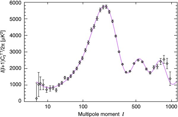
Figure 1. WMAP five-year temperature (TT) power spectrum. The red curve is the best-fit theory spectrum from the ΛCDM/WMAP chain (Dunkley et al. 2009, Table 2) based on WMAP alone, with parameters  . The uncertainties include both cosmic variance, which dominates below ℓ = 540, and instrumental noise which dominates at higher multipoles. The uncertainties increase at large ℓ due to WMAP's finite resolution. The improved resolution of the third peak near ℓ = 800 in combination with the simultaneous measurement of the rest of the spectrum leads to the improved results reported in this release.
Download figure:
Standard image High-resolution imageFigure 12 compares the unbinned five-year TT spectrum with the three-year result. Aside from the small upward shift of the five-year spectrum relative to that of the three-year, due to the new beam-transfer function, they are identical at low-ℓ. Figure 13 shows the unbinned TT spectrum broken down into its frequency components (V × V, V × W, W × W), demonstrating that the signal is independent of frequency.
How much has the determination of the third acoustic peak improved with the five-year data? Over the range ℓ = 680–900, which approximately spans the rise and fall of the third peak (from the bottom of the second trough to the point on the opposite side of the peak), the fiducial spectrum is preferred over a flat mean spectrum by Δχ2 = 7.6. For the three-year data it was Δχ2 = 3.6. With a few more years of data, WMAP should detect the curvature of third peak to greater than 3σ.
In Figure 2 we compare the WMAP five-year TT power spectrum along with recent results from other experiments (Readhead et al. 2004; Jones et al. 2006; Reichardt et al. 2008), showing great consistency between the various measurements. Several on-going and future ground-based CMB experiments plan on calibrating themselves off their overlap with WMAP at the highest-ℓ's; improving WMAP's determination of the third peak will have the added benefit of improving their calibrations.

Figure 2. WMAP five-year TT power spectrum along with recent results from the ACBAR (Reichardt et al. 2008, purple), Boomerang (Jones et al. 2006, green), and CBI (Readhead et al. 2004, red) experiments. The other experiments calibrate with WMAP or WMAP's measurement of Jupiter (CBI). The red curve is the best-fit ΛCDM model to the WMAP data, which agrees well with all datasets when extrapolated to higher ℓ.
Download figure:
Standard image High-resolution image3.1. Unresolved Point Source Correction
A population of point sources, Poisson-distributed over the sky, contributes an additional source of white noise to the measured TT power spectrum, CTTl → CTTl + Cps. Given a known source distribution N(>S), the number of sources per steradian with flux greater than S, the point-source-induced signal is
where S is the source flux, Sc is the flux cutoff (above which sources are masked and removed from the map), and g(ν) = (c2/2kν2)r(ν) converts flux density to thermodynamic temperature, with
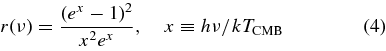
converting antenna to thermodynamic temperature.
At the frequencies and flux densities relevant for WMAP, source counts are dominated by flat-spectrum radio sources, which have flux spectra that are nearly constant with frequency (S ∼ να with α ≈ 0). Wright et al. (2009) find the average spectral index of sources bright enough to be detected in the WMAP five-year data to be 〈α〉 = −0.09, with an intrinsic dispersion of σα = 0.176. Since a source with flux S ∼ να has a thermodynamic temperature T ∼ να−2r(ν), we model the frequency dependence of Cps as
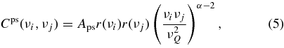
where νi,j are the frequencies of the two maps used to calculate the TT spectrum, Aps is an unknown amplitude, and νQ = 40.7 GHz is the Q-band central frequency.
In this section, we estimate the value of Aps needed to correct the TT power spectrum, finding Aps = 0.011 ± 0.001 μK2 sr, and discuss incorporating its uncertainty into the likelihood function.
3.1.1. Estimating the Correction
For a fixed beam size, flat-spectrum radio sources are much fainter in the W-band temperature maps than in Q- or V-band, allowing us to use the frequency dependence of the TT spectrum at high-ℓ to constrain the value of Aps. As in previous releases, the estimator we use is
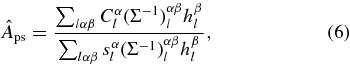
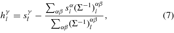
where Greek letters represent a pair of frequencies (e.g., VW), Cαl is the measured TT cross-power spectrum, Σαβl is the 〈CαlCβl〉 covariance matrix including cosmic variance and detector noise, and sαl = l(l + 1)Cps(α)/2π. The inverse estimator variance (![$[\delta \hat{A}_{{\rm ps}}]^{-2}$](https://content.cld.iop.org/journals/0067-0049/180/2/296/revision1/apjs291878ieqn3.gif) ) is given by the denominator of (6). While Σαβl does not include the off-diagonal coupling due to the mask, the diagonal elements are renormalized to account for the loss of sky coverage.
) is given by the denominator of (6). While Σαβl does not include the off-diagonal coupling due to the mask, the diagonal elements are renormalized to account for the loss of sky coverage.
Measured values for Aps are listed in Table 1 for various frequency combinations (QVW and VW) and galactic masks (KQ85, KQ80, and KQ75). The QVW estimates are insensitive to the galactic mask; the VW estimate increases somewhat as more of the sky is masked. Both the QVW and VW estimates prefer the same value (≈0.011 μK2 sr) of Aps when the KQ75 mask is used. While we restrict the data to ℓ = 300–800, the QVW estimate is only a weak function of the chosen ℓ-range; Figure 3 shows Aps estimated in bins of width Δℓ = 100. We adopt Aps = 0.011 ± 0.001 μK2 sr as our correction to the final combined TT spectrum. The consistency between ℓ-bins and between QVW and VW seen in Figure 3 is an important null test for the angular power spectrum. Aps (VW) is proportional to the power in the V–W map in a given ℓ-range. Figure 4 shows no evidence for any detectable residual signal in the VW maps after point source subtraction.
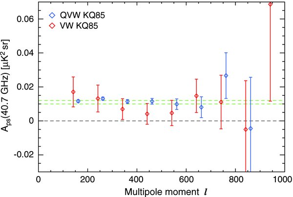
Figure 3. Unresolved point source contamination Aps, measured in bins of Δℓ = 100 evaluated at 40.7 GHz (Q band). For a source population whose fluxes are independent of frequency Aps scales roughly as ∼ν−2 in the WMAP data. The red data points are from the analysis of V and W bands alone and the blue points are from the analysis of Q, V, and W bands. The horizontal dashed green lines, at 0.010 and 0.012, show the 1σ bounds for our adopted value of Aps. Note that the QVW amplitude is independent of ℓ.
Download figure:
Standard image High-resolution image
Figure 4. TT V–W null spectrum. After correcting for unresolved point source emission, the individual power spectra are subtracted in power spectrum space. The result is consistent with zero and thus there is no evidence of point source contamination. In these units, point source contamination would be evident as a horizontal offset from zero. At ℓ = 500, the TT power spectrum is CTTℓ ≈ 0.06; thus the contamination is limited to roughly 3% in power.
Download figure:
Standard image High-resolution imageTable 1. Unresolved Point Source Contamination
| Bands | Mask | Aps(α = 0) (10−3 μK2 sr) | Aps(α = −0.09) (10−3 μK2 sr) |
|---|---|---|---|
| QVW | KQ85 | 11.3 ± 0.9 | 11.2 ± 0.9 |
| KQ80 | 11.3 ± 0.9 | 11.2 ± 0.9 | |
| KQ75 | 10.7 ± 1.0 | 10.6 ± 1.0 | |
| VW | KQ85 | 6.9 ± 3.4 | 7.2 ± 3.5 |
| KQ80 | 9.1 ± 3.6 | 9.5 ± 3.8 | |
| KQ75 | 10.5 ± 3.9 | 11.1 ± 4.1 |
Note. All results are for ℓ = 300–800.
Download table as: ASCIITypeset image
Because radio sources can only have positive flux they introduce a positive skewness to the maps, which can be detected in searches for non-Gaussianity. Komatsu et al. (2009) estimated the bispectrum induced by sources, finding bps = (4.3 ± 1.3) × 10−5 μK3 sr2 at Q band. Is this consistent with the value of Aps measured from the power spectrum? Given a theoretical model for the source number counts N(>S), one can predict the measured values of Cps and bps. Several models exist in the literature; we tested our results against two, Toffolatti et al. (1998, Tof98)18 and de Zotti et al. (2005, deZ05). Cps is calculated via (3), and bps from
where g(ν) and Sc are defined in (3). The comparison is complicated by the fact that Sc is unknown. We mask out not only the sources detected in WMAP data, but also undetected sources from external catalogues that are likely to contribute contaminating flux. However, a single value of Sc predicts both Cps and bps, so we can in principle tune Sc to match one, and see if it agrees with the other. In Table 2 we compare our measured values of Cps and bps with the rescaled Tof98 and deZ05 predictions for several values of Sc. There is some tension between the measured values and the model predictions. Given our measured value for bps the models would prefer a smaller value for Aps, in the range 0.008–0.010 μK2 sr. For the Tof98 model, the Sc ≈ 0.52 predictions are within 1σ of both Cps and bps. However, the deZ05 model appears to be discrepant, and a single value for Sc cannot match both Cps and bps.
Table 2. Unresolved Point Source Contamination
| Sc (Jy) | Cps (10−3 μK2 sr) | bps (10−5 μK3 sr2) | |
|---|---|---|---|
| WMAP5 (KQ75) | ⋅⋅⋅ | 11.7 ± 1.1a | 4.3 ± 1.3b |
| Toffolatti et al. (1998)×0.64 | 0.6 | 12.1 | 6.8 |
| 0.5 | 10.4 | 4.9 | |
| de Zotti et al. (2005) | 0.7 | 11.7 | 8.4 |
| 0.5 | 8.3 | 4.3 |
Notes. All numbers are evaluated at 40.7 GHz (Q band). aBy Equation (5), Cps(Q) = Apsr(Q)2 = 1.089 × Aps, where Aps is the QVW/KQ75 result from Table 1. bFrom Komatsu et al. (2009), using the Q-band map and KQ75 mask.
Download table as: ASCIITypeset image
Other groups have independently estimated the unresolved source contamination, and their results are in general agreement with ours. When the three-year data were initially released the correction was Aps = 0.017 ± 0.002 μK2 sr. Huffenberger et al. (2006) reanalyzed the data and claimed Aps = 0.011 ± 0.001, noticing that Aps was sensitive to the choice of galaxy mask; using the Kp0 mask instead of Kp2 reduced the value of Aps. Revisiting our original estimate for the three-year analysis, we reduced the correction to 0.014 ± 0.003 for the published papers. In a subsequent paper, Huffenberger et al. (2008), the same group corrected their original estimate after finding a small error, finding 0.013 ± 0.001, consistent with our published result.
4. TEMPERATURE-POLARIZATION SPECTRA
The standard model of adiabatic primordial density fluctuations predicts a correlation between the temperature and polarization fluctuations. The temperature traces primarily the density, and E-mode polarization the velocity, of the photon–baryon plasma at recombination. The correlation was seen in earlier WMAP data by Kogut et al. (2003) and Page et al. (2007). The anti-correlation near ℓ = 30 provides evidence that fluctuations exist on superhorizon scales, as is observed on an angular scale larger than the acoustic horizon at decoupling (Spergel & Zaldarriaga 1997b).
No significant changes have been made in the five-year TE analysis. We continue to use the method described by Page et al. (2007) to compute the TE power spectrum. The inputs are the KaQV polarization maps (Gold et al. 2009) and the VW temperature maps. For high multipoles ℓ>23, the likelihood can be approximated as a Gaussian, and we continue to use the ansatz given in Appendix C of Page et al. (2007) to compute the covariance matrix. At low multipoles, ℓ ⩽ 23, the likelihood of the polarization data is evaluated directly from the maps, following Appendix D in Page et al. (2007).
Figure 5 shows the TE spectrum. At low-ℓ the spectrum and error bars are approximated using the Gaussian form, although these are not used for cosmological analysis. With five years of data the anti-correlation at ℓ = 140 is clearly seen in the data, and the correlation at ℓ = 300 is measured with higher accuracy. The second anti-correlation at ℓ ∼ 450 is now better characterized, and is consistent with predictions of the ΛCDM model. The structure tests the consistency of the simple model, which fits both the TT and TE spectra with only six parameters. The best-fit ΛCDM model has χ2 = 415 for the TE component, with 421 degrees of freedom, giving χ2/ν = 0.99. The consistency confirms that the fluctuations are predominantly adiabatic, and constrains the amplitude of isocurvature modes.

Figure 5. WMAP five-year TE power spectrum. The green curve is the best-fit theory spectrum from the ΛCDM/WMAP Markov chain (Dunkley et al. 2009). For the TE component of the fit, χ2 = 415, and there are 427 multipoles and six parameters; thus the number of degrees of freedom is ν = 421, leading to χ2/ν = 0.99. The particle horizon size at decoupling corresponds to l ≈ 100. The clear anticorrelation between the primordial plasma density (corresponding approximately to T) and velocity (corresponding approximately to E) in causally disconnected regions of the sky indicates that the primordial perturbations must have been on a superhorizon scale. Note that the vertical axis is (ℓ + 1)Cℓ/(2π), and not ℓ(ℓ + 1)Cℓ/(2π).
Download figure:
Standard image High-resolution imageThe signal at the lowest multipoles, evaluated using the exact likelihood, is used to provide additional constraints on the reionization history. Although small, the measurement is consistent with the EE signal, and consistent with the three-year WMAP observations of Page et al. (2007). Dunkley et al. (2009) discuss constraints on reionization.
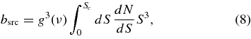
No correlation is expected between the temperature and the B-mode polarization. The TB spectrum is therefore primarily used as a null test, and is shown in Figure 6. It is consistent with no signal, as expected; over ℓ = 24–450 the reduced null χ2 is 0.97. This measurement is used in Komatsu et al. (2009) to place constraints on the presence of any parity violating terms coupled to photons, that could produce a TB correlation. We now include the TB spectrum at high-ℓ as an optional module for the likelihood code.
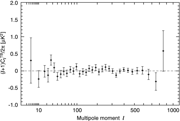
Figure 6. WMAP five-year TB power spectrum, showing no evidence of cosmological signal. The null reduced χ2 for ℓ = 24–450 is 0.97. Note that the vertical axis is (ℓ + 1)Cℓ/(2π), and not ℓ(ℓ + 1)Cℓ/(2π).
Download figure:
Standard image High-resolution image
Figure 7. Conditional likelihoods for the ℓ = 2–7 EE multipole moments (black curves), computed using the WMAP likelihood code by varying the multipole in question, with all other multipoles fixed to their fiducial values. For example, in the ℓ = 4 panel, the black curve is f(x) ∝ L(d|..., CEE3, CEE4 = x, CEE5, ...). For comparison, naïve pseudo-Cl estimates are also shown with Gaussian errors (red curves). The pseudo-Cℓ errors are noise only, while the conditional distributions include cosmic variance.
Download figure:
Standard image High-resolution imageTable 3. Beam/Source Likelihood Treatment Effect on Parameters
| Likelihood Treatment | ns | σ8 |
|---|---|---|
| Standard | 0.964 ± 0.014 | 0.796 ± 0.036 |
| SRCMARG | 0.964 ± 0.014 | 0.798 ± 0.036 |
| SRCMARG ×5 | 0.965 ± 0.015 | 0.803 ± 0.042 |
| BEAMMARG | 0.964 ± 0.015 | 0.799 ± 0.036 |
| BEAMMARG ×20 | 0.958 ± 0.016 | 0.796 ± 0.034 |
Notes. One-dimensional marginalized values for ns and σ8 for various treatments of the unresolved point source and beam uncertainty in the WMAP likelihood code. See Appendix A for descriptions of SRCMARG and BEAMMARG. Here, "×5" and "×20" indicate the error has been increased by a factor of 5 and 20, respectively.
Download table as: ASCIITypeset image
5. POLARIZATION SPECTRA
Due to its thermal stability (Jarosik et al. 2007) and well-characterized gain, WMAP can measure polarization signals even though the scan pattern was not optimized for doing so. The polarization signal is manifested in the time-ordered data (TOD) differently from the temperature signal. As a result, some of the low-ℓ polarization multipoles are well sampled and other multipoles are poorly sampled and have large statistical errors (Hinshaw et al. 2007; Page et al. 2007). This is a rather different situation than from that of the temperature spectrum, and the data must be analyzed with some care.
When we analyze the ℓ = 2 temperature power spectrum, we use the likelihood function rather than Gaussian errors, as the Gaussian approximation starts to break down with only ≈4 effective modes measured in the map (the reduction is due to fsky ≈ 0.7). For polarization, this effect is even more dramatic, as our scan pattern significantly lowers the effective number of multipoles measured, particularly for EE ℓ = 2, 5, 7, and 9 and BB ℓ = 3 (the peaks seen in Figure 16 in Page et al. 2007). Figure 8 demonstrates the importance of using the full likelihood description. The figure shows both the pseudo-Cl estimates of the ℓ = 2–7 BB multipoles and the conditional likelihoods computed using the WMAP likelihood code by varying the multipole in question, keeping the rest of the spectrum fixed to the fiducial best-fit ΛCDM model. From the plots it is clear that the best estimates of the mean and the uncertainty are not attained with the pseudo-Cl estimates.

Figure 8. Conditional likelihoods for the ℓ = 2–7 BB multipole moments (black curves), computed using the WMAP likelihood code by varying the multipole in question, with all other multipoles fixed to their fiducial values. For comparison, naïve pseudo-Cl estimates are also shown with Gaussian errors (red curves). The pseudo-Cℓ errors are noise only, while the conditional distributions include cosmic variance. Note the large difference between the likelihood code and the pseduo-Cℓ value for ℓ = 3; this mode is sensitive to the time-ordered data baseline and is extremely poorly measured by WMAP, illustrating the complicated noise structure of the polarization data on large scales.
Download figure:
Standard image High-resolution imageWe next consider the low-ℓ EE and BB power spectra in more detail. The low-ℓ EE power spectrum is shown in Figure 9. The uncertainties are obtained from the conditional likelihood and include cosmic variance; thus one cannot double the error flags to get the 95% confidence limits. If we zero out the ℓ < 10 portion of the fiducial EE and TE spectra the χ2 increases by 22.3, of which 2.7 is due to TE. Thus, the reionization feature in the EE power spectrum is preferred by Δχ2 = 19.6. The ℓ = 2, 3, 4, and 6 multipoles are cosmic variance limited, and the S/N for the combined ℓ = 2–7 bandpower is 11.
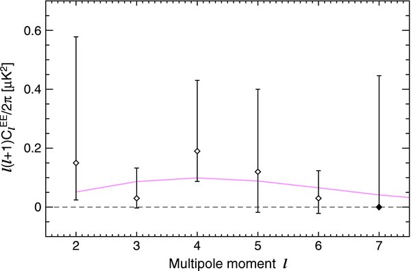
Figure 9. WMAP five-year EE power spectrum at low-ℓ. The error bars are the 68% CL of the conditional likelihood of each multipole, with the other multipoles fixed at their fiducial theory values; the diamonds mark the peak of the conditional likelihood distribution. The error bars include noise and cosmic variance; the point at ℓ = 7 is the 95% CL upper limit. The pink curve is the fiducial best-fit ΛCDM model (Dunkley et al. 2009).
Download figure:
Standard image High-resolution imageConsiderable effort has gone into understanding the W-band ℓ = 7 EE signal. Because of the apparent anomalously high-ℓ = 7 EE value computed by the pseudo-Cℓ algorithm, we have avoided using the W-band maps in cosmological analysis and use them only as an additional check on various models. Figure 8 of Hinshaw et al. (2009) shows that the ℓ = 7 value, while high, appears to be consistent with being in the tail of a properly computed likelihood distribution. The W-band ℓ = 7 problem may be a signature of poor statistics rather than a systematic. However, more data are needed to understand this potential anomaly. The ℓ = 3 BB signal gives perhaps the clearest example of the importance of using the full likelihood code. While the pseudo-Cl estimate implies a significant detection of power, the full likelihood code shows this to not be the case. The physical cause of the large uncertainty is that with our scan strategy an ℓ = 3 BB signal resembles an offset in the data and thus is not well separated from the baseline (Page et al. 2007; Hinshaw et al. 2009).
We see no evidence for a B-mode signal at low-ℓ, limiting the possible level to ℓ(ℓ + 1)CBBℓ=2−6/(2π) < 0.15 μK2 (95% CL), including cosmic variance. With τ = 0.1 and r = 0.2, a typical estimate for currently favored models of inflation, ℓ(ℓ + 1)CBBℓ=2−6/(2π) ≈ 0.008 μK2. Since a signal of 0.15 μK2 corresponds roughly to r ≈ 20, one can see that WMAP's limit is not based on the BB data, but on the tensor contribution to the TT and EE spectra as discussed by Komatsu et al. (2009).
For EE at ℓ>10, there are hints of signal in the data consistent with the standard ΛCDM model. However, the significance is not great enough to contribute to knowledge of the cosmological parameters. The five-year high-ℓ EE spectrum is shown in Figure 10, along with recent results from ground-based experiments (Leitch et al. 2005; Montroy et al. 2006; Sievers et al. 2007). For ℓ = 50–800, χ2 = 859.1 assuming CEEl = 0, and drops by 8.4, or almost 3σ, assuming the standard ΛCDM model. For the three-year data the equivalent change in χ2 was 6.2.

Figure 10. WMAP five-year EE power spectrum, compared with results from the Boomerang (Montroy et al. 2006, green), CAPMAP (Bischoff et al. 2008, orange), CBI (Sievers et al. 2007, red), DASI (Leitch et al. 2005, blue), and QUAD (Ade et al. 2008, purple) experiments. The pink curve is the best-fit theory spectrum from the ΛCDM/WMAP Markov chain (Dunkley et al. 2009). Note that the y-axis is CEEℓ, not ℓ(ℓ + 1)CEEℓ/(2π).
Download figure:
Standard image High-resolution imageThe high-ℓ BB spectrum is consistent with no signal, having a reduced χ2 of 1.02 over ℓ = 50–800 for the QV data. The lack of any signal in the low- and high-ℓ BB data is a necessary check of the foreground subtraction. As seen in Page et al. (2007), foreground emission produces E-modes and B-modes at similar levels; thus the absence of a B-mode signal suggests that the level of contamination in the E-mode signal is low. This is quantified by Dunkley et al. (2009).
6. SUMMARY AND CONCLUSIONS
We have presented the temperature and polarization angular power spectra of the CMB derived from the first five years of WMAP data. With greater integration time our determination of the third acoustic peak in the TT spectrum has improved. The low-ℓ reionization feature in the EE spectrum is now detected at nearly 5σ. The TB, EB, and BB spectra show no evidence for cosmological signal. The spectra are in excellent agreement with the best-fit ΛCDM model. Our knowledge of the power spectrum is improving both due to more detailed analyses, better modeling and understanding of the foreground emission, and more integration time.
All of the five-year WMAP data products are being made available through the Legacy Archive for Microwave Background Data Analysis (LAMBDA19), NASA's CMB Thematic Data Center. The temperature and polarization angular power spectra presented here are available, as is the WMAP likelihood code which incorporates our estimates of the Fisher matrix, point sources, and beam uncertainties.
The WMAP mission is made possible by the support of the Science Mission Directorate Office at NASA Headquarters. This research was additionally supported by NASA grants NNG05GE76G, NNX07AL75G S01, LTSA03-000-0090, ATPNNG04GK55G, and ADP03-0000-092. E.K. acknowledges support from an Alfred P. Sloan Research Fellowship. This research has made use of NASA's Astrophysics Data System Bibliographic Services. We acknowledge the use of the CAMB, CMBFAST, CosmoMC, and HEALPix (Gorski et al. 2005) software packages.
APPENDIX: LIKELIHOOD TREATMENT OF SOURCE/BEAM UNCERTAINTIES
In this appendix, we test the treatment of the unresolved source correction and beam uncertainties in the WMAP likelihood code, and show that it produces the correct results for cosmological parameters.
We adopt the same likelihood treatment of the unresolved point source correction uncertainty for the five-year likelihood code as used in the three-year code (Hinshaw et al. 2007, Appendix A), updated for the five-year value of Aps. Briefly, a correction to the logarithmic likelihood,  , where
  is the standard likelihood and
  is the combined source and beam correction, is calculated assuming the Cl are normally distributed, a reasonable assumption at high-ℓ.
Huffenberger et al. (2007, Huf08) disagreed with the source and beam likelihood module used in the three-year analysis, pointing out that the uncertainty in ns (the index of primordial scalar perturbations) was unchanged even if the uncertainty in Aps was increased by a factor of 100 (Figure 2 in their paper). They proposed an alternative approach, integrating the beam/point source covariance matrix into the cosmic variance/noise/mask covariance matrix and inverting the result in order to compute  directly, instead of calculating
  as a separate correction. Using this form of the likelihood, as δAps was increased, the uncertainty in ns increases (albeit modestly; δns increased by 38% when δAps → 100 × δAps).
However, while we agree that it is striking that the error in ns is seemingly unaffected by the uncertainty in Aps, we have some concerns regarding the Huf08 approach. To quote Huf08, "the errors on the source measurement do not make much difference, as long as [δAps] < 0.003[μK2 sr]," and their Figure 2 implies the same holds true when δAps = 0.003. This value is significant because it is the uncertainty adopted for the three-year WMAP analysis. When Huf08 adopted the same uncertainty, they found the same absolute uncertainty in ns as the WMAP team, but their central value was shifted higher by 0.005. This shift persisted as δAps → 0, and thus was seemingly not due to the point source uncertainty. The conclusion we draw is that they found the same value of δns as the WMAP three-year analysis, but their value of ns was biased high because of the way they treat the beam uncertainties. We believe the Huf08 value of ns would be in agreement with that found in WMAP3, but that it is biased high due to their treatment of beam uncertainties.
Huf08 quoted the value of  computed with their alternative likelihood module for a particular CMB spectrum distributed with the WMAP three-year likelihood code test program, finding
  , whereas the WMAP value is
  . As a check, we numerically marginalize the
  portion of the likelihood over beam and point source errors, to see if we can reproduce their value. The desired integral is
where
is the theoretical model (CTTl) perturbed by point source and beam errors. With 10 dimensions to integrate over (nine beam modes and one point source mode), normal grid-based quadrature is impractical, so we turn to Monte Carlo integration instead:
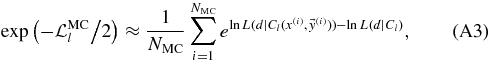
where x(i) and y(i)j are independent unit-variance normal deviates. With NMC = 104 points, we find  , consistent with the WMAP result of −1.22, but not the Huf08 result of −2.64.
As a further test of whether our cosmological parameter estimates fully capture the point source uncertainty, we have run a Markov chain with a modified form of the point source likelihood module, dubbed SRCMARG. The point source correction is calculated via a simple numerical integration,
with N = 25, Δ = 0.2, and wi = 1 except at the endpoints where w|N| = 1/2 (the trapezoidal rule). The resulting one-dimensional marginalized distribution for σ8, shown in the left panel of Figure 11, is indistinguishable from our standard result. We have also run a SRCMARG chain with the error increased by a factor of 5 (i.e., δAps = 0.005). In this case the uncertainty in σ8 increases by 15%.
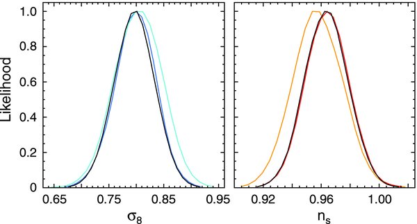
Figure 11. Left: one-dimensional marginalized likelihood distributions of σ8 for various treatments of the source uncertainty in the likelihood code: the standard likelihood function (black), the alternative treatment of the source uncertainty described in Equation (A5; blue), the alternative treatment, but with the unresolved point source error increased by ×5 (cyan). The agreement between black and blue curves shows that the standard treatment is producing the correct answer. Right: one-dimensional marginalized likelihood distributions of ns for various treatments of the beam uncertainties: the standard likelihood function (black), the alternative treatment of the beam uncertainty described in Equation (A5; red), the alternative treatment, but with the beam error increased by a factor of 20 (orange). The agreement between the black and red curves shows that the standard treatment is producing the correct answer.
Download figure:
Standard image High-resolution image
Figure 12. Unbinned WMAP five-year temperature (TT) power spectrum (black), compared with the WMAP three-year result (red). The slight upward shift of the five-year spectrum relative to the three-year spectrum is due to the change in the beam-transfer function. The pink curve is the best-fit ΛCDM model to the WMAP5 data.
Download figure:
Standard image High-resolution image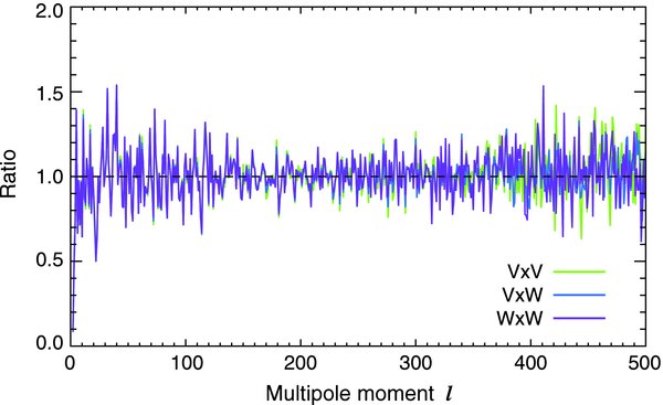
Figure 13. Unbinned WMAP five-year temperature (TT) power spectrum as a function of frequency, divided by the best-fit ΛCDM model to the WMAP data.
Download figure:
Standard image High-resolution image
Likewise, we have run similar tests of the beam uncertainty, dubbed BEAMMARG. The approach is the same as SRCMARG, but with "Cl + ασptsrcl" in (12) replaced by "Cl(1 + ασbeaml)," where σbeaml is the noisiest beam eigenmode, as shown in Figure 12 of Hill et al. (2009). The 1D marginalized distributions for ns are shown in the right panel of Figure 11. As with SRCMARG, the BEAMMARG result is indistinguishable from our standard result. Inflating the beam error by a factor of 20 results in a 14% increase in δns, along with a slight shift in ns away from unity.
Footnotes
- *
WMAP is the result of a partnership between Princeton University and NASA's Goddard Space Flight Center. Scientific guidance is provided by the WMAP Science Team.
- 15
Six of the sources in the five-year catalog were not added to the mask; they were found in a late update to the catalog after the mask had been finalized.
- 16
12,582,912 pixels (Nside = 1024).
- 17
The Markov chains in Dunkley et al. (2009) and Komatsu et al. (2009) were run with a version of the WMAP likelihood code with older and slightly larger values for fsky. The change in fsky increased the TT errors by on average 2%. Rerunning the ΛCDM chain with the new fsky leads to parameter shifts of at most 0.1σ.
- 18
- 19