


ABSTRACT
This paper focuses on cosmological constraints derived from analysis of WMAP data alone. A simple ΛCDM cosmological model fits the five-year WMAP temperature and polarization data. The basic parameters of the model are consistent with the three-year data and now better constrained: Ωbh2 = 0.02273 ± 0.00062, Ωch2 = 0.1099 ± 0.0062, ΩΛ = 0.742 ± 0.030, ns = 0.963+0.014−0.015, τ = 0.087 ± 0.017, and σ8 = 0.796 ± 0.036, with h = 0.719+0.026−0.027. With five years of polarization data, we have measured the optical depth to reionization, τ>0, at 5σ significance. The redshift of an instantaneous reionization is constrained to be zreion = 11.0 ± 1.4 with 68% confidence. The 2σ lower limit is zreion > 8.2, and the 3σ limit is zreion > 6.7. This excludes a sudden reionization of the universe at z = 6 at more than 3.5σ significance, suggesting that reionization was an extended process. Using two methods for polarized foreground cleaning we get consistent estimates for the optical depth, indicating an error due to the foreground treatment of τ ∼ 0.01. This cosmological model also fits small-scale cosmic microwave background (CMB) data, and a range of astronomical data measuring the expansion rate and clustering of matter in the universe. We find evidence for the first time in the CMB power spectrum for a nonzero cosmic neutrino background, or a background of relativistic species, with the standard three light neutrino species preferred over the best-fit ΛCDM model with Neff = 0 at >99.5% confidence, and Neff > 2.3(95%confidence limit (CL)) when varied. The five-year WMAP data improve the upper limit on the tensor-to-scalar ratio, r < 0.43(95%CL), for power-law models, and halve the limit on r for models with a running index, r < 0.58(95%CL). With longer integration we find no evidence for a running spectral index, with dns/dln k = −0.037 ± 0.028, and find improved limits on isocurvature fluctuations. The current WMAP-only limit on the sum of the neutrino masses is ∑mν < 1.3 eV(95%CL), which is robust, to within 10%, to a varying tensor amplitude, running spectral index, or dark energy equation of state.
Export citation and abstract BibTeX RIS
1. INTRODUCTION
The Wilkinson Microwave Anisotropy Probe (WMAP), launched in 2001, has mapped out the cosmic microwave background (CMB) with unprecedented accuracy over the whole sky. Its observations have led to the establishment of a simple concordance cosmological model for the contents and evolution of the universe, consistent with virtually all other astronomical measurements. The WMAP first-year and three-year data have allowed us to place strong constraints on the parameters describing the ΛCDM model, a flat universe filled with baryons, cold dark matter (CDM), neutrinos, and a cosmological constant, with initial fluctuations described by nearly scale-invariant power-law fluctuations, as well as placing limits on extensions to this simple model (Spergel et al. 2003, 2007). With all-sky measurements of the polarization anisotropy (Kogut et al. 2003; Page et al. 2007), 2 orders of magnitude smaller than the intensity fluctuations, WMAP has not only given us an additional picture of the universe as it transitioned from ionized to neutral at redshift z ∼ 1100, but also an observation of the later reionization of the universe by the first stars.
In this paper, we present cosmological constraints from WMAP alone, for both the ΛCDM model and a set of possible extensions. We also consider the consistency of WMAP constraints with other recent astronomical observations. This is one of the seven five-year WMAP papers. Hinshaw et al. (2009) describe the data processing and basic results, Hill et al. (2009) present new beam models and window functions, Gold et al. (2009) describe the emission from Galactic foregrounds, and Wright et al. (2009) describe the emission from extra-Galactic point sources. The angular power spectra are described by Nolta et al. (2009), and Komatsu et al. (2009) present and interpret cosmological constraints based on combining WMAP with other data.
WMAP observations are used to produce full-sky maps of the CMB in five frequency bands centered at 23, 33, 41, 61, and 94 GHz (Hinshaw et al. 2009). With five years of data, we are now able to place better limits on the ΛCDM model, as well as to move beyond it to test the composition of the universe, details of reionization, subdominant components, characteristics of inflation, and primordial fluctuations. We have more than doubled the amount of polarized data used for cosmological analysis, allowing a better measure of the large-scale E-mode signal (Nolta et al. 2009). To this end we test two alternative ways to remove Galactic foregrounds from low-resolution polarization maps, marginalizing over Galactic emission, providing a cross-check of our results. With longer integration we also better probe the second and third acoustic peaks in the temperature angular power spectrum, and have many more year-to-year difference maps available for cross-checking systematic effects (Hinshaw et al. 2009).
The paper is structured as follows. In Section 2 we focus on the CMB likelihood and parameter estimation methodology. We describe two methods used to clean the polarization maps, describe a fast method for computing the large-scale temperature likelihood, based on work described by Wandelt et al. (2004), which also uses Gibbs sampling, and outline more efficient techniques for sampling cosmological parameters. In Section 3 we present cosmological parameter results from five years of WMAP data for the ΛCDM model, and discuss their consistency with recent astronomical observations. Finally, we consider constraints from WMAP alone on a set of extended cosmological models in Section 4, and conclude in Section 5.
2. LIKELIHOOD AND PARAMETER ESTIMATION METHODOLOGY
2.1. Likelihood
The WMAP likelihood function takes the same format as for the three-year release, and software implementation is available on LAMBDA (http://lambda.gsfc.nasa.gov) as a standalone package. It takes in theoretical CMB temperature (TT), E-mode polarization (EE), B-mode polarization (BB), and temperature–polarization cross-correlation (TE) power spectra for a given cosmological model. It returns the sum of various likelihood components: low-ℓ temperature, low-ℓ TE/EE/BB polarization, high-ℓ temperature, high-ℓ TE cross-correlation, and additional terms due to uncertainty in the WMAP beam determination, and possible error in the extra-galactic point source removal. Now, there is also an additional option to compute the TB and EB likelihood. We describe the method used for computing the low-ℓ polarization likelihood in Section 2.1.1, based on maps cleaned by two different methods. The main improvement in the five-year analysis is the implementation of a faster Gibbs sampling method for computing the ℓ ⩽ 32 TT likelihood, which we describe in Section 2.1.2.
For ℓ>32, the TT likelihood uses the combined pseudo-Cℓ spectrum and covariance matrix described by Hinshaw et al. (2007), estimated using the V and W bands. We do not use the EE or BB power spectra at ℓ>23, but continue to use the TE likelihood described by Page et al. (2007), estimated using the Q and V bands. The errors due to beam and point sources are treated the same as in the three-year analysis, described in Appendix A of Hinshaw et al. (2007). A discussion of this treatment can be found in Nolta et al. (2009).
2.1.1. Low-ℓ Polarization Likelihood
We continue to evaluate the exact likelihood for the polarization maps at low multipole, ℓ ⩽ 23, as described in Appendix D of Page et al. (2007). The input maps and inverse covariance matrix used in the main analysis are produced by coadding the template-cleaned maps described by Gold et al. (2009). In both cases these are weighted to account for the P06 mask using the method described by Page et al. (2007). In the three-year analysis we conservatively used only the Q and V bands in the likelihood. We are now confident that the Ka band is cleaned sufficiently for inclusion in analyses (see Hinshaw et al. 2009 for a discussion).
We also cross-check the polarization likelihood by using polarization maps obtained with an alternative component-separation method, described by Dunkley et al. (2008). The low-resolution polarization maps in the K, Ka, Q, and V bands, degraded to HEALPix Nside = 8,15 are used to estimate a single set of marginalized Q and U CMB maps and associated inverse covariance matrix, that can then be used as inputs for the ℓ < 23 likelihood. This is done by estimating the joint posterior distribution for the amplitudes and spectral indices of the synchrotron, dust, and CMB Q and U components, using a Markov Chain Monte Carlo (MCMC) method. One then marginalizes over the foreground amplitudes and spectral indices to estimate the CMB component. A benefit of this method is that errors due to both instrument noise and foreground uncertainty are accounted for in the marginalized CMB covariance matrix.
2.1.2. Low-ℓ Temperature Likelihood
For a given set of cosmological parameters with theoretical power spectrum Cℓ, the likelihood function returns p(d|Cℓ), the likelihood of the observed map d, or its transformed alm coefficients. Originally, the likelihood code was written as a hybrid combination of a normal and log-normal distribution (Verde et al. 2003). This algorithm did not properly model the tails of the likelihood at low multipoles (Efstathiou 2004; Slosar et al. 2004; O'Dwyer et al. 2004; Hinshaw et al. 2007), and so for the three-year data the ℓ ⩽ 30 likelihood was computed exactly, using
where C is the covariance matrix of the data including both the signal covariance matrix and noise C(Cℓ) = S(Cℓ) + N (e.g., Tegmark 1997; Bond et al. 1998; Hinshaw et al. 2007). This approach is computationally intensive, however, since it requires the inversion of a large covariance matrix each time the likelihood is called.
In Jewell et al. (2004), Wandelt et al. (2004), and Eriksen et al. (2004a), a faster method was developed and implemented to compute p(d|Cℓ), which we now adopt. It is described in detail in those papers, so we only briefly outline the method here. The method uses Gibbs sampling to first sample from the joint posterior distribution p(Cℓ, s|d), where Cℓ is the power spectrum and s is the true sky signal. From these samples, a Blackwell–Rao (BR) estimator provides a continuous approximation to p(Cℓ|d). When a flat prior, p(Cℓ) = const, is used in the sampling, we have p(Cℓ|d) ∝ p(d|Cℓ), where the constant of proportionality is independent of Cℓ. The BR estimator can then be used as an accurate representation of the likelihood, p(d|Cℓ) (Wandelt et al. 2004; Chu et al. 2005).
The first step requires drawing samples from p(Cℓ, s|d). We cannot draw samples from the joint distribution directly, but we can from the two conditional distributions p(s|Cℓ, d) and p(Cℓ|s, d), each a slice through the (Np × ℓmax)-dimensional space. Samples are drawn alternately, forming a Markov Chain of points by the Gibbs algorithm. For the case of one Cℓ parameter and one s parameter the sampling goes as follows. We start from some arbitrary point (Ciℓ, si) in the parameter space, and then draw

by first drawing Ci + 1ℓ from p(Cℓ|si, d) and then drawing si + 1 from p(s|Ci + 1ℓ, d). Then we iterate many times. The result is a Markov chain whose stationary distribution is p(Cℓ, s|d). This is extended to vectors for Cℓ (of length ℓmax) and s (of length Np) following the same method:
sampling the joint distribution p(Cℓ, s|d). This sampling procedure is also described by Jewell et al. (2004), Wandelt et al. (2004), and Eriksen et al. (2007).
The first conditional distribution is a multivariate Gaussian with mean Si(Si + N)−1d and variance [(Si)−1 + N−1]−1, so at each step a new signal vector si + 1, of size Np, can be drawn. This is computationally demanding, however, as described by Eriksen et al. (2004a) and Wandelt et al. (2004), requiring the solution of a linear system of equations Mv = w, with M = 1 + S1/2N−1S1/2. These are solved at each step using the conjugate gradient technique, which is sped up by finding an approximate inverse for M, a preconditioner. This requires computation of the inverse noise matrix, N−1, in spherical harmonic space, which is done by computing the components of N−1 term-by-term using spherical harmonics in pixel space. There are more efficient ways to compute N−1 (Hivon et al. 2002; Eriksen et al. 2004b), but computing the preconditioner is a one-time expense, and it is only necessary to compute harmonics up to ℓ = 30.
The second conditional distribution, p(Cℓ|s, d), is an inverse Gamma distribution, from which a new Cℓ vector of size ℓmax can be rapidly drawn using the method by Wandelt et al. (2004). Sampling from these two conditional distributions is continued in turn until convergence, at which point the sample accurately represents the underlying distribution. This is checked in practice using a jacknife test that compares likelihoods from two different samples.
Finally, once the joint distribution p(Cℓ, s|d) has been pre-computed, the likelihood for any given model Cℓ is obtained by marginalizing over the signal s, p(d|Cℓ) ∝ ∫p(Cℓ, s|d)ds, which holds for a uniform prior distribution p(Cℓ). In practice this is computed using the BR estimator,
where the sum is over all nG samples in the Gibbs chain. Since p(Cℓ|si) = p(Cℓ|σiℓ), where σℓ = (2ℓ + 1)−1∑m|sℓm|2, and sℓm are the spherical harmonic coefficients of s, one only needs to store σiℓ at each step in the Gibbs sampling. Then, each time the likelihood is called for a new Cℓ, one computes  . This requires only O(ℓmaxnG) computations, compared to the full O(N3p) evaluation of Equation (1). This speed-up also means that the exact likelihood can be used to higher resolution than is feasible with the full evaluation, providing a more accurate estimation.
2.1.3. Code Details: Choice of ℓ Limits, Smoothing, and Resolution
The code used for WMAP is adapted from the MAGIC Gibbs code described by Wandelt (2003) and Wandelt et al. (2004). The input temperature map is the five-year internal linear combination (ILC) map described by Gold et al. (2009). To produce correct results, the Gibbs sampler requires an accurate model of the data. This means that the signal covariance matrix S(Cℓ) cannot be approximated to be zero except for multipoles where the smoothing makes the signal much less than the noise. For the full WMAP dataset, this would require sampling out to ℓ ∼ 1000, with Nside = 512. This is computationally expensive, taking more than of order 104 processor hours to converge (O'Dwyer et al. 2004). Instead we reduce the resolution and smooth the data to substantially reduce the required multipole range, speeding up the computation.
The ILC map is smoothed to 5° FWHM, and sampled at Nside = 32. The process of smoothing the data has the side effect of correlating the noise. Properly modeling the correlated noise slows down the Gibbs sampling, as it takes longer to draw a sample from p(s|Cℓ, d). We therefore add uncorrelated white noise to the map such that it dominates over the smoothed noise. However, the added noise must not be so large that it changes the likelihood of the low-ℓ modes; cosmic variance must remain dominant over the noise (Eriksen et al. 2007), so we add 2 μK of noise per pixel. In Appendix A the noise power spectra are shown.
The Gibbs sampler converges more slowly in regions of low signal-to-noise ratio (S/N). Because of this, we only sample spectra out to ℓ = 51 and fix the spectrum for 51 < ℓ ⩽ 96 to a fiducial value, and set it to zero for ℓ>96. The BR estimator is only used up to ℓ = 32 for cosmological analysis, so we marginalize over the 32 < ℓ ⩽ 51 spectrum. The likelihood is therefore p(L|d) = ∫p(L, H|d)dH, where L and H refer to the low, ℓ ⩽ 32, and higher, 32 < ℓ ⩽ 51, parts of the power spectrum. Examination of the BR estimator shows it to have a smooth distribution. Tests of the results to various input choices, including the choice of resolution, are given in Appendix A. We note that by using the low-ℓ likelihood only up to ℓ ⩽ 32, this breaks the likelihood into a low- and high-ℓ part, which introduces a small error by ignoring the correlation between these two parts of the spectrum. However, this error is small, and it is unfeasible, in a realistic sampling time, to use the BR estimator over the entire ℓ range probed by WMAP.
In Figure 1 we show slices through the Cℓ distribution obtained from the BR estimator, compared to the pixel likelihood code. The estimated spectra agree well. Some small discrepancies are due to the pixel code using Nside = 16, compared to the higher resolution Nside = 32 used for the Gibbs code.
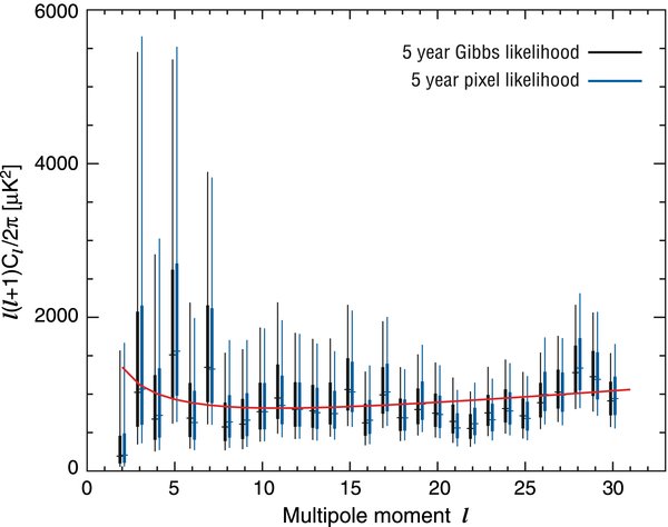
Figure 1. This figure compares the low-ℓ TT power spectrum computed with two different techniques. At each ℓ value, we plot the maximum likelihood value (tic mark), the region where the likelihood is greater than 50% of the peak value (thick line) and the region where the likelihood is greater than 95% of the peak value (thin line). The black lines (left side of each pair) are estimated by Gibbs sampling using the ILC map smoothed with a 5° Gaussian beam (at HEALPIX Nside = 32). The light blue line (right side of the pair) is estimated with a pixel-based likelihood code with Nside = 16. The slight differences between the points are primarily due to differences in resolution. At each multipole, the likelihood is sampled by fixing the other Cℓ values at a fiducial spectrum (red).
Download figure:
Standard image High-resolution image2.2. Parameter Estimation
We use the MCMC methodology described by Spergel et al. (2003, 2007) to explore the probability distributions for various cosmological models, using the five-year WMAP data and other cosmological datasets. We map out the full distribution for each cosmological model, for a given dataset or data combination, and quote parameter results using the means and 68% confidence limits (CL) of the marginalized distributions, with
where xji is the jth value of the ith parameter in the chain. We also give 95% upper or lower limits when the distribution is one-tailed. We have made a number of changes in the five-year analysis, outlined here and in Appendix B.
We parameterize our basic ΛCDM cosmological model in terms of the following parameters:

defined in Table 1.  is the amplitude of curvature perturbations and ns is the spectral tilt, both defined at the pivot scale k0 = 0.002 Mpc−1. In this simplest model we assume "instantaneous" reionization of the universe, with optical depth τ, in which the universe transitions from being neutral to fully ionized during a change in redshift of z = 0.5. The contents of the universe, assuming a flat geometry, are quantified by the baryon density ωb, the CDM density ωc, and a cosmological constant ΩΛ. We treat the contribution to the power spectrum by Sunyaev–Zel'dovich (SZ) fluctuations (Sunyaev & Zel'dovich 1970) as in Spergel et al. (2007), adding the predicted template spectrum from Komatsu & Seljak (2002), multiplied by an amplitude ASZ, to the total spectrum. This template spectrum is scaled with frequency according to the known SZ frequency dependence. We limit 0 < ASZ < 2 and impose unbounded uniform priors on the remaining six parameters.
We also consider extensions to this model, parameterized by

also defined in Table 1. These include cosmologies in which the primordial perturbations have a running scalar spectral index dns/dln k, a tensor contribution with tensor-to-scalar ratio r, or an anticorrelated or uncorrelated isocurvature component, quantified by α−1, α0. They also include models with a curved geometry Ωk, a constant dark energy equation of state w, and those with massive neutrinos ∑mν = 94Ωνh2eV, varying numbers of relativistic species Neff, and varying primordial helium fraction YP. There are also models with non-instantaneous "two-step" reionization as in Spergel et al. (2007), with an initial ionized step at zr with ionized fraction xe, followed by a second step at z = 7 to a fully ionized universe.
Table 1. Cosmological Parameters Used in the Analysis
| Parameter | Description |
| ωb | Baryon density, Ωbh2 |
| ωc | CDM density, Ωch2 |
| ΩΛ | Dark energy density, with w = −1 unless stated |
 |
Amplitude of curvature perturbations at k0 = 0.002 Mpc−1 |
| ns | Scalar spectral index at k0 = 0.002 Mpc−1 |
| τ | Reionization optical depth |
| ASZ | SZ marginalization factor |
| dns/dln k | Running in scalar spectral index |
| r | Ratio of the amplitude of tensor fluctuations to scalar fluctuations |
| α−1 | Fraction of anticorrelated CDM isocurvature (see Section 4.1.3) |
| α0 | Fraction of uncorrelated CDM isocurvature (see Section 4.1.3) |
| Neff | Effective number of relativistic species (assumed neutrinos) |
| ων | Massive neutrino density, Ωνh2 |
| Ωk | Spatial curvature, 1 − Ωtot |
| w | Dark energy equation of state, w = pDE/ρDE |
| YP | Primordial helium fraction |
| xe | Ionization fraction of first step in two-step reionization |
| zr | Reionization redshift of first step in two-step reionization |
| σ8 | Linear theory amplitude of matter fluctuations on 8 h−1 Mpc scales |
| H0 | Hubble expansion factor (100 h Mpc−1 km s−1) |
| ∑mν | Total neutrino mass (eV) ∑mν = 94Ωνh2 |
| Ωm | Matter energy density Ωb + Ωc + Ων |
| Ωmh2 | Matter energy density |
| t0 | Age of the universe (billions of years) |
| zreion | Redshift of instantaneous reionization |
| η10 | Ratio of baryon-to-photon number densities, 1010(nb/nγ) = 273.9Ωbh2 |
Note. http://lambda.gsfc.nasa.gov lists the marginalized values for these parameters for all of the models discussed in this paper.
Download table as: ASCIITypeset image
These parameters all take uniform priors, and are all sampled directly, but we bound Neff < 10, w > − 2.5, zr < 30 and impose positivity priors on r, α−1, α0, ων, Yp, and ΩΛ, as well as requiring 0 < xe < 1. The tensor spectral index is fixed at nt = −r/8. We place a prior on the Hubble constant of 20 < H0 < 100, but this only affects nonflat models. Other parameters, including σ8, the redshift of reionization, zreion, and the age of the universe, t0, are derived from these primary parameters and described in Table 1. A more extensive set of derived parameters are provided on the LAMBDA Web site. In this paper we assume that the primordial fluctuations are Gaussian, and do not consider constraints on parameters describing deviations from Gaussianity in the data. These are discussed in the cosmological interpretation presented by Komatsu et al. (2009).
We continue to use the CAMB code (Lewis et al. 2000), based on the CMBFAST code (Seljak & Zaldarriaga 1996), to generate the CMB power spectra for a given set of cosmological parameters.16 Given the improvement in the WMAP data, we have determined that distortions to the spectra due to weak gravitational lensing should now be included (see, e.g.; Blanchard & Schneider 1987; Seljak 1997; Hu & Okamoto 2002). We use the lensing option in CAMB which roughly doubles the time taken to generate a model, compared to the unlensed case.
We have made a number of changes in the parameter-sampling methodology. Our main pipeline now uses an MCMC code originally developed for use in Bucher et al. (2004), which has been adapted for WMAP. For increased speed and reliability, it incorporates two changes in the methodology described by Spergel et al. (2007). It uses a modified sampling method that generates a single chain for each model (instead of the four, or eight, commonly used in cosmological analyses). We also use an alternative spectral convergence test that can be run on a single chain, developed by Dunkley et al. (2005), instead of the Gelman & Rubin test used in Spergel et al. (2007). These are both described in Appendix B. We also use the publicly available CosmoMC sampling code (Lewis & Bridle 2002) as a secondary pipeline, used as an independent cross-check for a limited set of models.
3. THE ΛCDM COSMOLOGICAL MODEL
3.1. WMAP Five-Year Parameters
The ΛCDM model, described by just six parameters, is still an excellent fit to the WMAP data. The temperature and polarization angular power spectra are shown by Nolta et al. (2009). With more observation the errors on the third acoustic peak in the temperature angular power spectrum have been reduced. The TE cross-correlation spectrum has also improved, with a better measurement of the second anticorrelation at ℓ ∼ 500. The low-ℓ signal in the EE spectrum, due to reionization of the universe (Ng & Ng 1995; Zaldarriaga & Seljak 1997), is now measured with higher significance (Nolta et al. 2009). The best-fit six-parameter model, shown in Figure 2, is successful in fitting three TT acoustic peaks, three TE cross-correlation maxima/minima, and the low-ℓ EE signal. The model is compared to the polarization data in Nolta et al. (2009). The consistency of both the temperature and polarization signals with ΛCDM continues to validate the model.
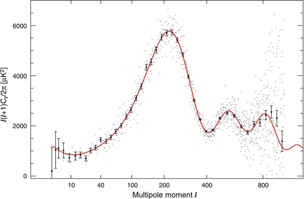
Figure 2. Temperature angular power spectrum corresponding to the WMAP-only best-fit ΛCDM model. The gray dots are the unbinned data; the black data points are binned data with 1σ error bars including both noise and cosmic variance computed for the best-fit model.
Download figure:
Standard image High-resolution imageThe five-year marginalized distributions for ΛCDM, shown in Table 2 and Figures 3 and 4, are consistent with the three-year results (Spergel et al. 2007), but the uncertainties are all reduced, significantly so for certain parameters. With longer integration of the large-scale polarization anisotropy, there has been a significant improvement in the measurement of the optical depth to reionization. There is now a 5σ detection of τ, with mean value τ = 0.087 ± 0.017. This can be compared to the three-year measure of τ = 0.089 ± 0.03. The central value is little altered with two more years of integration, and the inclusion of the Ka band data, but the limits have almost halved. This measurement, and its implications, are discussed in Section 3.1.1.

Figure 3. Constraints on ΛCDM parameters from the five-year WMAP data. The two-dimensional 68% and 95% marginalized limits are shown in blue. They are consistent with the three-year constraints (gray). Tighter limits on the amplitude of matter fluctuations, σ8, and the CDM density Ωch2, arise from a better measurement of the third temperature (TT) acoustic peak. The improved measurement of the EE spectrum provides a 5σ detection of the optical depth to reionization, τ, which is now almost uncorrelated with the spectral index ns.
Download figure:
Standard image High-resolution image
Figure 4. Constraints from the five-year WMAP data on ΛCDM parameters (blue), showing marginalized one-dimensional distributions and two-dimensional 68% and 95% limits. Parameters are consistent with the three-year limits (gray) from Spergel et al. (2007), and are now better constrained.
Download figure:
Standard image High-resolution imageTable 2. ΛCDM Model Parameters and 68% Confidence Intervals From the Five-Year WMAP Data Alone
| Parameter | Three-Year Mean | Five-Year Mean | Five-Year Max Like |
|---|---|---|---|
| 100Ωbh2 | 2.229 ± 0.073 | 2.273 ± 0.062 | 2.27 |
| Ωch2 | 0.1054 ± 0.0078 | 0.1099 ± 0.0062 | 0.108 |
| ΩΛ | 0.759 ± 0.034 | 0.742 ± 0.030 | 0.751 |
| ns | 0.958 ± 0.016 | 0.963+0.014−0.015 | 0.961 |
| τ | 0.089 ± 0.030 | 0.087 ± 0.017 | 0.089 |
 |
(2.35 ± 0.13) × 10−9 | (2.41 ± 0.11) × 10−9 | 2.41 × 10⁻⁹ |
| σ8 | 0.761 ± 0.049 | 0.796 ± 0.036 | 0.787 |
| Ωm | 0.241 ± 0.034 | 0.258 ± 0.030 | 0.249 |
| Ωmh2 | 0.128 ± 0.008 | 0.1326 ± 0.0063 | 0.131 |
| H0 | 73.2+3.1−3.2 | 71.9+2.6−2.7 | 72.4 |
| zreion | 11.0 ± 2.6 | 11.0 ± 1.4 | 11.2 |
| t0 | 13.73 ± 0.16 | 13.69 ± 0.13 | 13.7 |
Notes. The three-year values are shown for comparison. For best estimates of parameters, the marginalized "Mean" values should be used. The "Max Like" values correspond to the single model giving the highest likelihood.
Download table as: ASCIITypeset image
The higher acoustic peaks in the TT and TE power spectra also provide more information about the ΛCDM model. Longer integration has resulted in a better measure of the height and position of the third peak. The highest multipoles have a slightly higher mean value relative to the first peak, compared to the three-year data. This can be attributed partly to improved beam modeling, and partly to longer integration time reducing the noise. The third peak position constrains Ω0.275mh, while the third peak height strongly constrains the matter density, Ωmh2 (Hu & White 1996; Hu & Sugiyama 1995). In this region of the spectrum, the WMAP data are noise-dominated so that the errors on the angular power spectrum shrink as 1/t. The uncertainty on the matter density has dropped from 12% in the first-year data to 8% in the three-year data and now 6% in the five-year data. The CDM density constraints are compared to three-year limits in Figure 3. The spectral index still has a mean value 2.5σ less than unity, with ns = 0.963+0.014−0.015. This continues to indicate the preference of a red spectrum consistent with the simplest inflationary scenarios (Linde 2005; Boyle et al. 2006), and our confidence will be enhanced with more integration time.
Both the large-scale EE spectrum and the small-scale TT spectrum contribute to an improved measure of the amplitude of matter fluctuations. With the CMB we measure the amplitude of curvature fluctuations, quantified by  , but we also derive limits on σ8, the amplitude of matter fluctuations on 8h−1Mpc scales. A higher value for τ produces more overall damping of the CMB temperature signal, making it somewhat degenerate with the amplitude,
  , and therefore σ8. The value of σ8 also affects the height of the acoustic peaks at small scales, so information is gained from both temperature and polarization. The five-year data give σ8 = 0.796 ± 0.036, slightly higher than the three-year result, driven by the increase in the amplitude of the power spectrum near the third peak. The value is now remarkably consistent with new measurements from weak lensing surveys, as discussed in Section 3.2.
3.1.1. Reionization
Our observations of the acoustic peaks in the TT and TE spectrum imply that most of the ions and electrons in the universe combined to make neutral hydrogen and helium at z ≃ 1100. Observations of quasar spectra show diminishing Gunn–Peterson troughs at z < 5.8 (Fan et al. 2000, 2001) implying that the universe was nearly fully ionized by z = 5.7. How did the universe make the transition from being nearly fully neutral to fully ionized? The astrophysics of reionization has been a very active area of research in the past decade. Several recent reviews (Barkana & Loeb 2006; Fan et al. 2006; Furlanetto et al. 2006; Meiksin 2007) summarize the current observations and theoretical models. Here, we highlight a few of the important issues and discuss some of the implications of the WMAP measurements of optical depth.
What objects reionized the universe? While high-redshift galaxies are usually considered the most likely source of reionization, active galactic nuclei (AGNs) may also have played an important role. As galaxy surveys push toward ever higher redshift, it is unclear whether the known population of star-forming galaxies at z ∼ 6 could have ionized the universe (see, e.g. Bunker et al. 2007). The EE signal clearly seen in the WMAP five-year data (2008, Section 2) implies an optical depth, τ ≃ 0.09. This large optical depth suggests that higher redshift galaxies, perhaps the low-luminosity sources appearing in z > 7 surveys (Stark et al. 2007), played an important role in reionization. While the known population of AGNs cannot be a significant source of reionization (Bolton & Haehnelt 2007; Srbinovsky & Wyithe 2007), an early generation of supermassive black holes could have played a role in reionization (Ricotti & Ostriker 2004; Ricotti et al. 2007). This early reionization would also have an impact on the CMB.
Most of our observational constraints probe the end of the epoch of reionization. Observations of z > 6 quasars (Becker 2001; Djorgovski et al. 2001; Fan et al. 2006; Willott et al. 2007) find that the Lyα optical depth rises rapidly. Measurements of the afterglow spectrum of a gamma-ray burst at z = 6.3 (Totani et al. 2006) suggest that universe was mostly ionized at z = 6.3. Lyα emitter surveys (Taniguchi et al. 2005; Malhotra & Rhoads 2006; Kashikawa et al. 2006; Iye et al. 2006; Ota et al. 2008) imply a significant ionized fraction at z = 6.5. The interpretation that there is a sudden change in the properties of the intergalactic medium (IGM) remains a subject of active debate (Becker et al. 2007; Wyithe et al. 2008).
The WMAP data place new constraints on the reionization history of the universe. The WMAP data best constrains the optical depth due to reionization at moderate redshift (z < 25) and only indirectly constrains the redshift of reionization. If reionization is sudden, then the WMAP data imply that zreion = 11.0 ± 1.4, as shown in Figure 5, and now excludes zreion = 6 at more than 99.9% CL. The combination of the WMAP data implying that the universe was mostly reionized at z ∼ 11 and the measurements of rapidly rising optical depth at z ∼ 6–6.5 suggest that reionization was an extended process rather than a sudden transition. Many early studies of reionization envisioned a rapid transition from a neutral to a fully ionized universe occurring as ionized bubbles percolate and overlap. As Figure 5 shows, the WMAP data suggest a more gradual process with reionization beginning perhaps as early as z ∼ 20 and strongly favoring z > 6. This suggests that the universe underwent an extended period of partial reionization. The limits were found by modifying the ionization history in CAMB to include two steps in the ionization fraction at late times (z < 30): the first at zr with ionization fraction xe, the second at z = 7 with xe = 1. Several studies (Cen 2003; Chiu et al. 2003; Wyithe & Loeb 2003; Haiman & Holder 2003; Yoshida et al. 2004; Choudhury & Ferrara 2006; Iliev et al. 2007; Wyithe et al. 2008) suggest that feedback produces a prolonged or perhaps even, multiepoch reionization history.
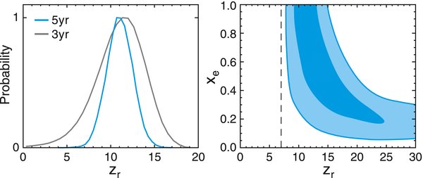
Figure 5. Left: marginalized probability distribution for zreion in the standard model with instantaneous reionization. Sudden reionization at z = 6 is ruled out at 3.5σ, suggesting that reionization was a gradual process. Right: in a model with two steps of reionization (with ionization fraction xe at redshift zr, followed by full ionization at z = 7), the WMAP data are consistent with an extended reionization process.
Download figure:
Standard image High-resolution imageWhile the current WMAP data constrain the optical depth of the universe, the EE data does not yet provide a detailed constraint on the reionization history. With more data from WMAP and upcoming data from Planck, the EE spectrum will begin to place stronger constraints on the details of reionization (Kaplinghat et al. 2003; Holder et al. 2003; Mortonson & Hu 2008). These measurements will be supplemented by measurements of the Ostriker–Vishniac effect by high-resolution CMB experiments which is sensitive to ∫n2edt (Ostriker & Vishniac 1986; Jaffe & Kamionkowski 1998; Gruzinov & Hu 1998), and discussed in, e.g., Zhang et al. (2004).
3.1.2. Sensitivity to Foreground Cleaning
As the E-mode signal is probed with higher accuracy, it becomes increasingly important to test how much the constraint on τ, zreion, and the other cosmological parameters, depend on details of the Galactic foreground removal. Tests were done by Page et al. (2007) to show that τ was insensitive to a set of variations in the dust template used to clean the maps. In Figure 6 we show the effect on ΛCDM parameters of changing the number of bands used in the template-cleaning method: discarding the Ka band in the "QV" combination, or adding the W band in the "KaQVW" combination. We find that τ (and therefore zreion) is sensitive to the maps, but the dispersion is consistent with noise. As expected, the error bars are broadened for the QV-combined data, and the mean value is τ = 0.080 ± 0.020. When the W band is included, the mean value is τ = 0.100 ± 0.015. We choose not to use the W-band map in our main analysis, however, because there appears to be excess power in the cleaned map at ℓ = 7. This indicates a potential systematic error, and is discussed further by Hinshaw et al. (2009). The other cosmological parameters are only mildly sensitive to the number of bands used. This highlights the fact that τ is no longer as strongly correlated with other parameters, as in earlier WMAP data (Spergel et al. 2003, 2007), notably with the spectral index of primordial fluctuations, ns (Figure 3).
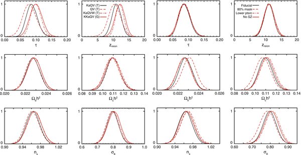
Figure 6. Effect of foreground treatment and likelihood details on ΛCDM parameters. Left: the number of bands used in the template cleaning (denoted "T") affects the precision to which τ is determined, with the standard KaQV compared to QV and KaQVW, but has little effect on other cosmological parameters. Using maps cleaned by Gibbs sampling (KKaQV (G)) also gives consistent results. Right: lowering the residual point source contribution (denoted lower ptsrc) and removing the marginalization over an SZ contribution (no SZ) affects parameters by <0.4σ. Using a larger mask (80% mask) has a greater effect, increasing Ωbh2 by 0.5σ, but is consistent with the effects of noise.
Download figure:
Standard image High-resolution imageWe also test the parameters obtained using the Gibbs-cleaned maps described by Dunkley et al. (2008) and in Section 2.1.1, which use the K, Ka, Q, and V band maps. Their mean distributions are also shown in Figure 6, and have mean optical depth less than 1σ higher than the KaQV template-cleaned maps, obtained using an independent method. The other cosmological parameters are changed by less than 0.3σ compared to the template-cleaned results. This consistency gives us confidence that the parameter constraints are little affected by foreground uncertainty. The difference in central values from the two methods indicates an error due to foreground removal uncertainty on τ, in addition to the statistical error, of ∼0.01.
3.1.3. Sensitivity to Likelihood Details
The likelihood code used for cosmological analysis has a number of variable components that have been fixed using our best estimates. Here we consider the effect of these choices on the five-year ΛCDM parameters. The first two are the treatment of the residual point sources, and the treatment of the beam error, both discussed by Nolta et al. (2009). The multifrequency data are used to estimate a residual point source amplitude of Aps = 0.011 ± 0.001 μK2sr, which scales the expected contribution to the cross-power spectra of sources below our detection threshold. It is defined by Hinshaw et al. (2007) and Nolta et al. (2009), and is marginalized over in the likelihood code. The estimate comes from QVW data, whereas the VW data give 0.007 ± 0.003 μK2sr, both using the KQ85 mask described by Hinshaw et al. (2009). The right panels in Figure 6 shows the effect on a subset of parameters of lowering Aps to the VW value, which leads to a slightly higher ns, Ωch2, and σ8, all within 0.4σ of the fiducial values, and consistent with more of the observed high-ℓ signal being due to CMB rather than unresolved point sources. We also use Aps = 0.011 μK2sr with no point source error, and find a negligible effect on parameters (<0.1σ). The beam window function error is quantified by 10 modes, and in the standard treatment we marginalize over them, following the prescription by Hinshaw et al. (2007). We find that removing the beam error also has a negligible effect on parameters. This is discussed further by Nolta et al. (2009), who consider alternative treatments of the beam and point source errors.
The next issue is the treatment of a possible contribution from SZ fluctuations. We account for the SZ effect in the same way as in the three-year analysis, marginalizing over the amplitude of the contribution parameterized by the Komatsu–Seljak model (Komatsu & Seljak 2002). The parameter ASZ is unconstrained by the WMAP data, but is not strongly degenerate with any other parameters. In Figure 6 we show the effect on parameters of setting the SZ contribution to zero. Similar to the effect of changing the point source contribution, the parameters depending on the third peak are slightly affected, with a <0.25σ increase in ns, Ωch2, σ8, and a similar decrease in the baryon density.
Another choice is the area of sky used for cosmological interpretation, or how much we mask out to account for Galactic contamination. Gold et al. (2009) discuss the new masks used for the five-year analysis, with the KQ85 mask used as standard. We test the effect of using the more conservative KQ80 mask, and find a more noticeable shift. The quantity Ωbh2 is increased by 0.5σ, and ns, Ωch2, and σ8 all decreased by ∼0.4σ. This raised concerns that the KQ85 mask contains residual foreground contamination, but as discussed by Nolta et al. (2009), this shift is found to be consistent with the effects of noise, tested with simulations. We also confirm that the effect on parameters is even less for ΛCDM models using WMAP with external data, and that the choice of mask has only a small effect on the tensor amplitude, raising the 95% confidence level by ∼5%.
Finally, we test the effect on parameters of varying aspects of the low-ℓ TT treatment. These are discussed in Appendix B, and in summary we find the same parameter results for the pixel-based likelihood code compared to the Gibbs code, when both use ℓ ⩽ 32. Changing the mask at low-ℓ to KQ80, or using the Gibbs code up to ℓ ⩽ 51, instead of ℓ ⩽ 32, has a negligible effect on parameters.
3.2. Consistency of the ΛCDM Model with Other Datasets
While the WMAP data alone place strong constraints on cosmological parameters, there has been a wealth of results from other cosmological observations in the last few years. These observations can generally be used either to show consistency of the simple ΛCDM model parameters, or to constrain more complicated models. In this section we compare a broad range of current astronomical data to the WMAP ΛCDM model. A subset of the data is used to place combined constraints on extended cosmological models in Komatsu et al. (2009). For this subset, we describe the methodology used to compute the likelihood for each case, but do not report on the joint constraints in this paper.
3.2.1. Small-Scale CMB Measurements
A number of recent CMB experiments have probed smaller angular scales than WMAP can reach and are therefore more sensitive to the higher order acoustic oscillations and the details of recombination (e.g., Hu & Sugiyama 1994, 1996; Hu & White 1997). Since the three-year WMAP analysis, there have been new temperature results from the Arcminute Cosmology Bolometer Array Receiver (ACBAR), both in 2007 (Kuo et al. 2007) and in 2008 (Reichardt et al. 2008). They have measured the angular power spectrum at 145 GHz to 5' resolution, over ∼ 600 deg2. Their results are consistent with the model predicted by the WMAP five-year data, shown in Figure 7, although ACBAR is calibrated using WMAP, so the data are not completely independent.
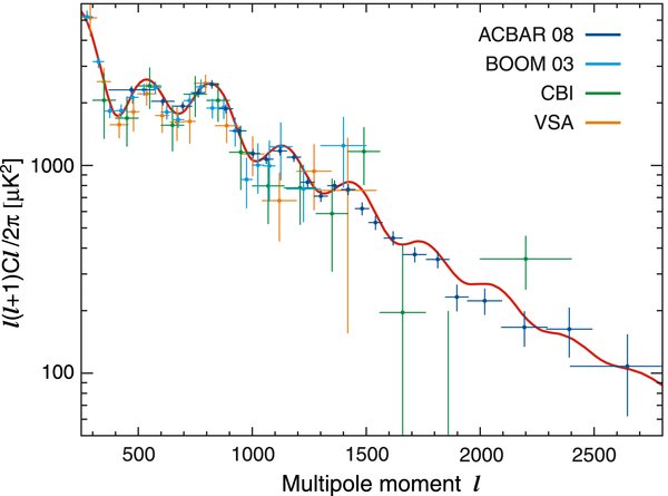
Figure 7. Best-fit temperature angular power spectrum from WMAP alone (red), which is consistent with data from recent small-scale CMB experiments: ACBAR, CBI, VSA, and BOOMERANG.
Download figure:
Standard image High-resolution imageFigure 7 also shows data from the BOOMERANG, Cosmic Background Imager (CBI), and Very Small Array (VSA) experiments, which agree well with WMAP. There have also been new observations of the CMB polarization from two ground-based experiments, QUaD, operating at 100 and 150 GHz (Ade et al. 2008), and CAPMAP, at 40 and 100 GHz (Bischoff et al. 2008). Their measurements of the EE power spectrum are shown by Nolta et al. (2009), together with detections already made since 2005 (Leitch et al. 2005; Sievers et al. 2007; Barkats et al. 2005; Montroy et al. 2006), and are all consistent with the ΛCDM model parameters.
In our combined analysis in Komatsu et al. (2009) we use two different data combinations. For the first we combine four datasets. This includes the 2007 ACBAR data (Kuo et al. 2007), using 10 bandpowers in the range 900 < ℓ < 2000. The values and errors were obtained from the ACBAR Web site. We also include the three external CMB datasets used in Spergel et al. (2003): the CBI (Mason et al. 2003; Sievers et al. 2003; Pearson et al. 2003; Readhead et al. 2004), the VSA (Dickinson et al. 2004), and BOOMERANG (Ruhl et al. 2003; Montroy et al. 2006; Piacentini et al. 2006). As in the three-year release we only use bandpowers that do not overlap with the signal-dominated WMAP data, due to nontrivial cross-correlations, so we use seven bandpowers for CBI (in the range 948 < ℓ < 1739), five for VSA (894 < ℓ < 1407), and seven for BOOMERANG (924 < ℓ < 1370), using the log-normal form of the likelihood. Constraints are also found by combining WMAP with the 2008 ACBAR data, using 16 bandpowers in the range 900 < ℓ < 2000. In this case the other CMB experiments are not included. We do not use additional polarization results for parameter constraints as they do not yet improve limits beyond WMAP alone.
3.2.2. Baryon Acoustic Oscillations (BAO)
The acoustic peak in the galaxy correlation function is a prediction of the adiabatic cosmological model (Peebles & Yu 1970; Sunyaev & Zel'dovich 1970; Bond & Efstathiou 1984; Hu & Sugiyama 1996). It was first detected using the Sloan Digital Sky Survey (SDSS) luminous red galaxy (LRG) survey, using the brightest class of galaxies at mean redshift z = 0.35 by Eisenstein et al. (2005). The peak was detected at 100 h−1 Mpc separation, providing a standard ruler to measure the ratio of distances to z = 0.35 and the CMB at z = 1089, and the absolute distance to z = 0.35. More recently, Percival et al. (2007b) have obtained a stronger detection from over half a million SDSS main galaxies and LRGs in the DR5 sample. They detect BAO with over 99% confidence. A combined analysis was then undertaken of SDSS and Two Degree Field Galaxy Redshift Survey (2dFGRS) by Percival et al. (2007a). They find evidence for BAO in three catalogs: at mean redshift z = 0.2 in the SDSS DR5 main galaxies plus the 2dFGRS galaxies, at z = 0.35 in the SDSS LRGs, and in the combined catalog. Their data are shown in Figure 8, together with the WMAP best-fit model. The BAO are shown by dividing the observed and model power spectra by P(k)smooth, a smooth cubic spline fit described by Percival et al. (2007a). The observed power spectra are model-dependent, but were calculated using Ωm = 0.25 and h = 0.72, which agrees with our maximum-likelihood model.
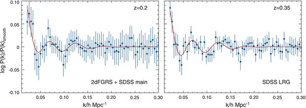
Figure 8. BAO expected for the best-fit ΛCDM model (red lines), compared to BAO in galaxy power spectra calculated from (left) combined SDSS and 2dFGRS main galaxies, and (right) SDSS LRG galaxies, by Percival et al. (2007a). The observed and model power spectra have been divided by P(k)smooth, a smooth cubic spline fit described by Percival et al. (2007a).
Download figure:
Standard image High-resolution imageThe scale of the BAO is analyzed to estimate the geometrical distance measure at z = 0.2 and z = 0.35,

where DA is the angular diameter distance and H(z) is the Hubble parameter. They find rs/DV(0.2) = 0.1980 ± 0.0058 and rs/DV(0.35) = 0.1094 ± 0.0033. Here, rs is the comoving sound horizon scale at recombination. Our ΛCDM model, using the WMAP data alone, gives rs/DV(0.2) = 0.1946 ± 0.0079 and rs/DV(0.35) = 0.1165 ± 0.0042, showing the consistency between the CMB measurement at z = 1089 and the late-time galaxy clustering. However, while the z = 0.2 measures agree to within 1σ, the z = 0.35 measurements have mean values almost 2σ apart. The BAO constraints are tighter than the WMAP predictions, which shows that they can improve upon the WMAP parameter determinations, in particular on ΩΛ and Ωmh2.
In Komatsu et al. (2009) the combined bounds from both surveys are used to constrain models as described by Percival et al. (2007a), adding a likelihood term given by −2ln L = XTC−1X, with

and C11 = 35, 059, C12 = −24, 031, C22 = 108, 300, including the correlation between the two measurements. Komatsu et al. (2009) also consider constraints using the SDSS LRG limits derived by Eisenstein et al. (2005), using the combination
for z = 0.35 and computing a Gaussian likelihood

3.2.3. Galaxy Power Spectra
We can compare the predicted fluctuations from the CMB to the shape of galaxy power spectra, in addition to the scale of acoustic oscillations (e.g., Eisenstein & Hu 1998). The SDSS galaxy power spectrum from DR3 (Tegmark et al. 2004) and the 2dFGRS spectrum (Cole et al. 2005) were shown to be in good agreement with the WMAP three-year data, and used to place tighter constraints on cosmological models (Spergel et al. 2007), but there was some tension between the preferred values of the matter density (Ωm = 0.236 ± 0.020 for WMAP combined with 2dFGRS and 0.265 ± 0.030 with SDSS). Recent studies used photometric redshifts to estimate the galaxy power spectrum of LRGs in the range 0.2 < z < 0.6 from the SDSS fourth data release (DR4), finding Ωm = 0.30 ± 0.03 (for h = 70, Padmanabhan et al. 2007) and Ωmh = 0.195 ± 0.023 for h = 0.75 (Blake et al. 2007).
More precise measurements of the LRG power spectrum were obtained from redshift measurements: Tegmark et al. (2006) used LRGs from SDSS DR4 in the range 0.01 h Mpc−1 < k < 0.2 h Mpc−1 combined with the three-year WMAP data to place strong constraints on cosmological models. However, there is a disagreement between the matter density predicted using different minimum scales, if the nonlinear modeling used by Tegmark et al. (2006) is adopted. Using the three-year WMAP data combined with the LRG spectrum we find Ωm = 0.228 ± 0.019, using scales with k < 0.1 h Mpc−1, and Ωm = 0.248 ± 0.018 for k < 0.2 h Mpc−1. These constraints are obtained for the six-parameter ΛCDM model, following the nonlinear prescription described by Tegmark et al. (2006). The predicted galaxy power spectrum Pg(k) is constructed from the "dewiggled" linear matter power spectrum Pm(k) using Pg(k) = b2Pm(k)(1 + Qk2)/(1 + 1.4k), and the parameters b and Q are marginalized over. The dewiggled spectrum is a weighted sum of the matter power spectrum at z = 0 and a smooth power spectrum (Tegmark et al. 2006). Without this dewiggling, we find Ωm = 0.246 ± 0.018 for k < 0.2 h Mpc−1, so its effect is small. We also explored an alternative form for the bias, motivated by third-order perturbation theory analysis, with Pg(k) = b2Pnlm(k) + N (see, e.g. Seljak 2001; Schulz & White 2006). Here, Pnlm is the nonlinear matter power spectrum using the Halofit model (Smith et al. 2003) and N is a constant accounting for nonlinear evolution and scale-dependent bias. Marginalizing over b and N we still find a discrepancy with scale, with Ωm = 0.230 ± 0.021 using scales with k < 0.1 h Mpc−1, and Ωm = 0.249 ± 0.018 for k < 0.2 h Mpc−1. Constraints using this bias model are also considered in Hamann et al. (2008a). These findings are consistent with results obtained from the DR5 main galaxy and LRG sample (Percival et al. 2007c), who argue that this shows evidence for scale-dependent bias on large scales, which could explain the observed differences in the early SDSS and 2dFGRS results. While this will likely be resolved with future modeling and observations, we choose not to use the galaxy power spectra to place joint constraints on the models reported by Komatsu et al. (2009).
3.2.4. Type Ia Supernovae
In the last decade, Type Ia supernovae have become an important cosmological probe, and have provided the first direct evidence for the acceleration of the universe by measuring the luminosity distance as a function of redshift. The observed dimness of high-redshift supernovae (z ∼ 0.5) was first measured by Riess et al. (1998), Schmidt et al. (1998), and Perlmutter et al. (1999), confirmed with more recent measurements including those of Nobili et al. (2005), Krisciunas et al. (2005), Clocchiatti et al. (2006), and Astier et al. (2006), and extended to higher redshift by Riess et al. (2004) who found evidence for the earlier deceleration of the universe. The sample of high-redshift supernovae has grown by over 80 since the three-year WMAP analysis. Recent HST measurements of 21 new high-redshift supernova by Riess et al. (2007) include 13 at z > 1, allowing the measurement of the Hubble expansion H(z) at distinct epochs and strengthening the evidence for a period of deceleration followed by acceleration. The ESSENCE Supernova Survey has also recently reported results from 102 supernovae discovered from 2002 to 2005 using the 4-m Blanco Telescope at the Cerro Tololo Inter-American Observatory (Miknaitis et al. 2007), of which 60 are used for cosmological analysis (Wood-Vasey et al. 2007). A combined cosmological analysis was performed for a subset of the complete supernova dataset by Davis et al. (2007) using the MCLS2k2 light curve fitter (Jha et al. 2007). More recently, a broader "Union" compilation of the currently observed SNIa, including a new nearby sample, was analyzed by Kowalski et al. (2008) using the SALT1 light curve fitter (Guy et al. 2005).
In Figure 9, we confirm that the recently observed supernovae are consistent with the ΛCDM model, which predicts the luminosity distance μth as a function of redshift and is compared to the Union combined dataset (Kowalski et al. 2008). In the cosmological analysis described by Komatsu et al. (2009), the Union data is used, consisting of 307 supernovae that pass various selection cuts. These include supernovae observed using the HST (Riess et al. 2007), from the ESSENCE survey (Miknaitis et al. 2007), and the Supernova Legacy Survey (SNLS; Astier et al. 2006). For each supernova the luminosity distance predicted from theory is compared to the observed value. This is derived from measurements of the apparent magnitude m and the inferred absolute magnitude M, to estimate a luminosity distance μobs = 5log[dL(z)/Mpc] + 25. The likelihood is given by
summed over all supernovae, where a single absolute magnitude is marginalized over (Lewis & Bridle 2002), and σobs is the observational error accounting for extinction, intrinsic redshift dispersion, K-correction, and light curve stretch factors.

Figure 9. Red line shows the luminosity–distance relationship predicted for the best-fit WMAP-only model (the right column in Table 2). The points show binned supernova observations from the Union compilation (Kowalski et al. 2008), including high-redshift SNIa from Hubble Space Telescope (HST; Riess et al. 2007), ESSENCE (Miknaitis et al. 2007), and SNLS (Astier et al. 2006). The plot shows the deviation of the luminosity distances from the empty universe model.
Download figure:
Standard image High-resolution image3.2.5. Hubble Constant Measurements
The WMAP estimated value of the Hubble constant, H0 = 71.9+2.6−2.7 km s−1 Mpc−1, assuming a flat geometry, is consistent with the HST Key Project measurement of 72 ± 8 km s−1 Mpc−1 (Freedman et al. 2001). It also agrees within 1σ with measurements from gravitationally lensed systems (Koopmans et al. 2003), SZ and X-ray observations (Bonamente et al. 2006), Cepheid distances to nearby galaxies (Riess et al. 2005), the distance to the Maser-host galaxy NGC4258 as a calibrator for the Cepheid distance scale (Macri et al. 2006), and a new measure of the Tully–Fisher zero point (Masters et al. 2006), the latter two giving H0 = 74 ± 7 km s−1 Mpc−1. Lower measures are favored by a compilation of the Cepheid distance measurements for 10 galaxies using the HST by Sandage et al. (2006; H0 = 62 ± 6 km s−1 Mpc−1), and new measurements of an eclipsing binary in M33 which reduce the Key Project measurement to H0 = 61 km s−1 Mpc−1 (Bonanos et al. 2006). Higher measures are found using revised parallaxes for Cepheids (van Leeuwen et al. 2007), raising the Key Project value to 76 ± 8 km s−1 Mpc−1. In Komatsu et al. (2009) the Hubble Constant measurements are included for a limited set of parameter constraints, using the Freedman et al. (2001) measurement as a Gaussian prior on H0.
3.2.6. Weak Lensing
Weak gravitational lensing is produced by the distortion of galaxy images by the mass distribution along the line of sight (see Refregier 2003 for a review). There have been significant advances in its measurement in recent years, and in the understanding of systematic effects (e.g., Massey et al. 2007), and intrinsic alignment effects (Hirata et al. 2007), making it a valuable cosmological probe complementary to the CMB. Early results by the RCS (Hoekstra et al. 2002), VIRMOS-DESCART (Van Waerbeke et al. 2005), and the Canada–France–Hawaii Telescope Legacy Survey (CFHTLS; Hoekstra et al. 2006) lensing surveys favored higher amplitudes of mass fluctuations than preferred by WMAP. However, new measurements of the two-point correlation functions from the third year CFHTLS Wide survey (Fu et al. 2008) favor a lower amplitude consistent with the WMAP measurements, as shown in Table 3. This is due to an improved estimate of the galaxy redshift distribution from CFHTLS-Deep (Ilbert et al. 2006), compared to that obtained from photometric redshifts from the small Hubble Deep Field, which were dominated by systematic errors. Their measured signal agrees with results from the 100 Square Degree Survey (Benjamin et al. 2007), a compilation of data from the earlier CFHTLS-Wide, RCS, and VIRMOS-DESCAT surveys, together with the GABoDS survey (Hetterscheidt et al. 2007), with average source redshift z ∼ 0.8. Both these analyses rely on a two-dimensional measurement of the shear field. Cosmic shear has also been measured in two and three dimensions by the HST COSMOS survey (Massey et al. 2007), using redshift information to providing an improved measure of the mass fluctuation. Their measures are somewhat higher than the WMAP value, as shown in Table 3, although not inconsistent. Weak lensing is also produced by the distortion of the CMB by the intervening mass distribution (Zaldarriaga & Seljak 1999; Hu & Okamoto 2002), and can be probed by measuring the correlation of the lensed CMB with tracers of large-scale structure. Two recent analyses have found evidence for the cross-correlated signal (Smith et al. 2007; Hirata et al. 2008), both consistent with the five-year WMAP ΛCDM model. They find a 3.4σ detection of the correlation between the three-year WMAP data and NRAO VLA Sky Survey (NVSS) radio sources (Smith et al. 2007), and a correlation at the 2.1σ level of significance between WMAP and data from NVSS, and from SDSS LRGs and quasars (Hirata et al. 2008).
Table 3. Measurements of Combinations of the Matter Density, Ωm, and Amplitude of Matter Fluctuations, σ8, From Weak Lensing Observations (Fu et al. 2008; Benjamin et al. 2007; Massey et al. 2007), Compared to WMAP
| Data | Parameter | Lensing Limits | Five-Year WMAP Limits |
|---|---|---|---|
| CFHTLS Wide | σ8(Ωm/0.25)0.64 | 0.785 ± 0.043 | 0.814 ± 0.090 |
| 100 Sq Deg | σ8(Ωm/0.24)0.59 | 0.84 ± 0.07 | 0.832 ± 0.088 |
| COSMOS 2D | σ8(Ωm/0.3)0.48 | 0.81 ± 0.17 | 0.741 ± 0.069 |
| COSMOS 3D | σ8(Ωm/0.3)0.44 | 0.866+0.085−0.068 | 0.745 ± 0.067 |
Download table as: ASCIITypeset image
3.2.7. Integrated Sachs–Wolfe Effect
Correlation between large-scale CMB temperature fluctuations and large-scale structure is expected in the ΛCDM model due to the change in gravitational potential as a function of time, and so provides a test for dark energy (Boughn et al. 1998). Evidence of a correlation was found in the first-year WMAP data (e.g., Boughn & Crittenden 2004; Nolta et al. 2004). Two recent analyses combine recent large-scale structure data (Two Micron All Sky Survey, SDSS LRGs, SDSS quasars, and NVSS radio sources) with the WMAP three-year data, finding a 3.7σ (Ho et al. 2008) and 4σ (Giannantonio et al. 2008) detection of ISW at the expected level. Other recent studies using individual datasets find a correlation at the level expected with the SDSS DR4 galaxies (Cabré et al. 2006), at high redshift with SDSS qusars (Giannantonio et al. 2006), and with the NVSS radio galaxies (Pietrobon et al. 2006; McEwen et al. 2007).
3.2.8. Lyα Forest
The Lyα forest seen in quasar spectra probes the underlying matter distribution on small scales (Rauch 1998). However, the relationship between absorption line structure and mass fluctuations must be fully understood to be used in a cosmological analysis. The power spectrum of the Lyα forest has been used to constrain the shape and amplitude of the primordial power spectrum (Viel et al. 2004; McDonald et al. 2005; Seljak et al. 2005; Desjacques & Nusser 2005), and recent results combine the three-year WMAP data with the power spectrum obtained from the LUQAS sample of VLT-UVES spectra (Viel et al. 2006) and SDSS QSO spectra (Seljak et al. 2006). Both groups found results suggesting a higher value for σ8 than consistent with WMAP. However, measurements by Kim et al. (2007) of the probability distribution of the Lyα flux have been compared to simulations with different cosmological parameters and thermal histories (Bolton et al. 2008). They imply that the temperature–density relation for the IGM may be close to isothermal or inverted, which would result in a smaller amplitude for the power spectrum than previously inferred, more in line with the five-year WMAP value of σ8 = 0.796 ± 0.036. Simulations in larger boxes by Tytler et al. (2007) fail to match the distribution of flux in observed spectra, providing further evidence of disagreement between simulation and observation. Given these uncertainties, the Lyα forest data are not used for the main results presented by Komatsu et al. (2009). However, constraints on the running of the spectral index are discussed, using data described by Seljak et al. (2006). With more data and further analyses, the Lyα forest measurements can potentially place powerful constraints on the neutrino mass and a running spectral index.
3.2.9. Big Bang Nucleosynthesis (BBN)
WMAP measures the baryon abundance at decoupling, with Ωbh2 = 0.02273 ± 0.00062, giving a baryon-to-photon ratio of η10(WMAP) = 6.225 ± 0.170. Element abundances of deuterium, helium, and lithium also depend on the baryon abundance in the first few minutes after the big bang. Steigman (2007) reviews the current status of BBN measurements. Deuterium measurements provide the strongest test, and are consistent with WMAP, giving η10(D) = 6.0 ± 0.4 based on new measurements by O'Meara et al. (2006). The 3He abundance is more poorly constrained at η10(3He) = 5.6+2.2−1.4 from the measure of y3 = 1.1 ± 0.2 by Bania et al. (2002). The neutral lithium abundance, measured in low-metallicity stars, is two times smaller than the CMB prediction, η(Li), from measures of the logarithmic abundance, [Li]P = 12 + log10(Li/H), in the range [Li]P ∼ 2.1–2.4 (Charbonnel & Primas 2005; Meléndez & Ramírez 2004; Asplund et al. 2005). These measurements could be a signature of new early universe physics, e.g., Coc et al. (2004), Richard et al. (2005), and Jedamzik (2004), with recent attempts to simultaneously fit both the 7Li and 6Li abundances by Bird et al. (2008), Jedamzik (2008a, 2008b), Cumberbatch et al. (2007), and Jittoh et al. (2008). The discrepancy could also be due to systematics, destruction of lithium in an earlier generation of stars, or uncertainties in the stellar temperature scale (Fields et al. 2005; Steigman 2006; Asplund et al. 2005). A possible solution has been proposed using observations of stars in the globular cluster NGC 6397 (Korn et al. 2006, 2007). They find evidence that as the stars age and evolve toward hotter surface temperatures, the surface abundance of lithium in their atmospheres drops due to atomic diffusion. They infer an initial lithium content of the stars [Li]P = 2.54 ± 0.1, giving η10(Li) = 5.4 ± 0.6 in good agreement with BBN predictions. However, further observations are needed to determine whether this scenario explains the observed uniform depletion of primordial 7Li as a function of metallicity. The measured abundance of 4He is also lower than predicted, with η10(4He) = 2.7+1.2−0.9 from a measure of YP = 0.240 ± 0.006, incorporating data from Izotov & Thuan (2004), Olive & Skillman (2004), and Gruenwald et al. (2002) by Steigman (2007). However, observations by Peimbert et al. (2007) and Fukugita & Kawasaki (2006) predict higher values more consistent with WMAP.
3.2.10. Strong Lensing
The number of strongly lensed quasars has the potential to probe cosmology, as a dark-energy-dominated universe predicts a large number of gravitational lenses (Turner 1990; Fukugita et al. 1990). The CLASS radio band survey has a large statistical sample of radio lenses (Myers et al. 2003; Koopmans et al. 2003; York et al. 2005), yielding estimates for ΩΛ ≃ 0.72–0.78 (Mitchell et al. 2005; Chae 2007). Oguri et al. (2008) have recently analyzed the large statistical lens sample from the Sloan Digital Sky Quasar Lens Search (Oguri et al. 2006). For w = −1, flat cosmology, they find ΩΛ = 0.74+0.11−0.15(stat.)+0.13−0.06(syst.). These values are all consistent with our best-fit cosmology. The abundance of giant arcs also has the potential to probe the underlying cosmology. However, although recent surveys have detected larger numbers of giant arcs (Gladders et al. 2003; Sand et al. 2005; Hennawi et al. 2008) than argued to be consistent with ΛCDM (Li et al. 2006; Broadhurst & Barkana 2008), numerical simulations (Meneghetti et al. 2007; Hennawi et al. 2007; Hilbert et al. 2007; Neto et al. 2007) find that the lens cross-sections are sensitive to the mass distribution in clusters as well as to the baryon physics (Wambsganss et al. 2007; Hilbert et al. 2008). These effects must be resolved in order to test ΛCDM consistency.
3.2.11. Galaxy Clusters
Clusters are easily detected and probe the high-mass end of the mass distribution, so probe the amplitude of density fluctuations and of large-scale structure. Cluster observations at optical wavelengths provided some of the first evidence for a low-density universe with the current preferred cosmological parameters (see, e.g., Fan et al. 1997). Observers are now using a number of different techniques for identifying cluster samples: large optical samples, X-ray surveys, lensing surveys (see, e.g., Wittman et al. 2006), and SZ surveys. The ongoing challenge is to determine the selection function and the relationship between astronomical observables and mass. This has recently seen significant progress in the optical (Lin et al. 2006; Sheldon et al. 2007; Reyes et al. 2008; Rykoff et al. 2008) and the X-ray (Sheldon et al. 2001; Reiprich & Böhringer 2002; Kravtsov et al. 2006; Arnaud et al. 2007; Hoekstra 2007). With large new optical cluster samples (Bahcall et al. 2003; Hsieh et al. 2005; Miller et al. 2005; Koester et al. 2007) and X-ray samples from ROSAT, XMM-LSS, and Chandra (Pierre et al. 2006; Burenin et al. 2007; Vikhlinin et al. 2008), cosmological parameters can be further tested, and most recent results for σ8 are converging on values close to the WMAP best-fit value of σ8 = 0.796 ± 0.036. Constraints from the RCS survey (Gladders et al. 2007) give Ωm = 0.30+0.12−0.11 and σ8 = 0.70+0.27−0.1. Rozo et al. (2007) argue for σ8 > 0.76 (95% CL) from SDSS BCG samples. Mantz et al. (2008) find Ωm = 0.27+0.06−0.05 and σ8 = 0.77+0.07−0.06 for a flat model based on the Jenkins et al. (2001) mass function and the Reiprich & Böhringer (2002) mass–luminosity calibration. With a 30% higher zero point, Rykoff et al. (2008) find that their data are best fit by σ8 = 0.85 and Ωm = 0.24. Bergé et al. (2007) report σ8 = 0.92+0.26−0.30 for Ωm = 0.24 from their joint CFHTLS/XMM-LSS analysis. In Rines et al. (2007) redshift data from SDSS DR4 is used to measure virial masses for a large sample of X-ray clusters. For Ωm = 0.3, they find σ8 = 0.84 ± 0.03.
3.2.12. Galaxy Peculiar Velocities
With deep large-scale structure surveys, cosmologists have now been able to measure β, the amplitude of redshift space distortions as a function of redshift. Combined with a measurement of the bias, b, this yields a determination of the growth rate of structure f ≡ dln G/dln a = βb, where G is the growth factor. For Einstein gravity theories we expect f ≃ Ωγ with γ ≃ 6/11 (see Polarski & Gannouji 2008 for a more accurate fitting function). Analysis of redshift space distortions in the 2dFGRS (Peacock et al. 2001; Verde et al. 2002; Hawkins et al. 2003) find β = 0.47 ± 0.08 at z ≃ 0.1, consistent with the ΛCDM predictions for the best-fit WMAP parameters. The Tegmark et al. (2006) analysis of the SDSS LRG sample finds β = 0.31 ± 0.04 at z = 0.35. The Ross et al. (2007) analysis of the 2dF-SDSS LRG sample find β = 0.45 ± 0.05 at z = 0.55. The Guzzo et al. (2008) analysis of 10,000 galaxies in the VIMOS-VLT Deep Survey finds that β = 0.70 ± 0.26 at z = 0.8 and infer dln G/dln a = 0.91 ± 0.36, consistent with the more rapid growth due to matter domination at this epoch expected in a ΛCDM model. The da Ângela et al. (2008) analysis of a QSO sample finds β = 0.60+0.14−0.11 at z = 1.4 and use the clustering length to infer the bias. Extrapolating back to z = 0, they find a matter density of Ωm = 0.25+0.09−0.07. A second approach is to use objects with well-determined distances, such as galaxies and supernovae, to look for deviations from the Hubble flow (Strauss & Willick 1995; Dekel 2000; Zaroubi et al. 2001; Riess et al. 1995; Haugbølle et al. 2007). The Park & Park (2006) analysis of the peculiar velocities of galaxies in the SFI sample find σ8Ω0.6m = 0.56+0.27−0.21. Gordon et al. (2007) correlate peculiar velocities of nearby supernova and find σ8 = 0.79 ± 0.22. These measurements provide an independent consistency check of the ΛCDM model (see Nesseris & Perivolaropoulos 2008 for a recent review).
4. EXTENDED COSMOLOGICAL MODELS WITH WMAP
The WMAP data place tight constraints on the simplest ΛCDM model parameters. In this section we describe to what extent WMAP data constrain extensions to the simple model, in terms of quantifying the primordial fluctuations and determining the composition of the universe beyond the standard components. Komatsu et al. (2009) present constraints for WMAP combined with other data, and offer a more detailed cosmological interpretation of the limits.
4.1. Primordial Perturbations
4.1.1. Tensor Fluctuations
In the ΛCDM model, primordial scalar fluctuations are adiabatic and Gaussian, and can be described by a power-law spectrum,
producing CMB angular power spectra consistent with the data. Limits can also be placed on the amplitude of tensor fluctuations, or gravitational waves, that could have been generated at very early times. They leave a distinctive large-scale signature in the polarized B-mode of the CMB (e.g., Basko & Polnarev 1980; Bond & Efstathiou 1984) that provides a clean way to distinguish them from scalar fluctuations. However, we have not yet reached sensitivities to strongly constrain this signal with the polarization data from WMAP. Instead we use the tensor contribution to the temperature fluctuations at large scales to constrain the tensor-to-scalar ratio r. We define  , where Δ2h is the amplitude of primordial gravitational waves (see Komatsu et al. 2009), and choose a pivot scale k0 = 0.002 Mpc−1.
The WMAP data now constrain r < 0.43(95%CL). This is an improvement over the three-year limit of r < 0.65 (95% CL), and comes from the more accurate measurement of the second and third acoustic peaks. The dependence of the tensor amplitude on the spectral index is shown in Figure 10, showing the ns − r degeneracy (Spergel et al. 2007): a larger contribution from tensors at large scales can be offset by an increased spectral index, and an overall decrease in the amplitude of fluctuations, shown in Table 4. The degeneracy is partially broken with a better measure of the TT spectrum. There is a significant improvement in the limit on models whose scalar fluctuations can vary with scale, with a power spectrum with a "running" spectral index,
The limit from WMAP is now r < 0.58(95%CL), about half the three-year value r < 1.1 (Spergel et al. 2007).

Figure 10. Two-dimensional marginalized constraints (68% and 95% CLs) on inflationary parameters r, the tensor-to-scalar ratio, and ns, the spectral index of fluctuations, defined at k0 = 0.002 Mpc−1. One-dimensional 95% upper limits on r are given in the legend. Left: the five-year WMAP data place stronger limits on r (shown in blue) than three-year data (gray). This excludes some inflationary models including λϕ4 monomial inflaton models with r ∼ 0.27, ns ∼ 0.95 for 60 e-folds of inflation. Right: for models with a possible running spectral index, r is now more tightly constrained due to measurements of the third acoustic peak. Note: the two-dimensional 95% limits correspond to Δ(2ln L) ∼ 6, so the curves intersect the r = 0 line at the ∼2.5σ limits of the marginalized ns distribution.
Download figure:
Standard image High-resolution imageTable 4. Selection of Cosmological Parameter Constraints for Extensions to the ΛCDM Model Including Tensors and/or a Running Spectral Index
| Parameter | Tensors | Running | Tensors+Running |
| r | <0.43(95%CL) | <0.58(95%CL) | |
| dns/dln k | −0.037 ± 0.028 | −0.050 ± 0.034 | |
| ns | 0.986 ± 0.022 | 1.031+0.054−0.055 | 1.087+0.072−0.073 |
| σ8 | 0.777+0.040−0.041 | 0.816 ± 0.036 | 0.800 ± 0.041 |
Download table as: ASCIITypeset image
What do these limits tell us about the early universe? For models that predict observable gravitational waves, it allows us to exclude more of the parameter space. The simplest inflationary models predict a nearly scale-invariant spectrum of gravitational waves (Grishchuk 1975; Starobinsky 1979). In a simple classical scenario where inflation is driven by the potential V(ϕ) of a slowly rolling scalar field, the predictions (Lyth & Riotto 1999) are


for V(ϕ) ∝ ϕα, where N is the number of e-folds of inflation between the time when the horizon scale modes left the horizon and the end of inflation. For N = 60, the λϕ4 model with r ≃ 0.27, ns ≃ 0.95 is now excluded with more than 95% confidence. An m2ϕ2 model with r ≃ 0.13, ns ≃ 0.97 is still consistent with the data. Komatsu et al. (2009) discuss in some detail what these measurements, and constraints for combined datasets, imply for a large set of possible inflationary models and potentials.
With r = 0 also fitting the data well, models that do not predict an observable level of gravitational waves, including multi-field inflationary models (Polarski & Starobinsky 1995; Garcia-Bellido & Wands 1996), D-brane inflation (Baumann & McAllister 2007), and ekpyrotic or cyclic scenarios (Khoury et al. 2001; Boyle et al. 2004), are not excluded if one fits for both tensors and scalars.
4.1.2. Scale Dependence of Spectral Index
The running of the spectral index has been the subject of some debate in light of WMAP observations, with the three-year data giving limits of dns/dln k = −0.055 ± 0.030, showing some preference for decreasing power on small scales (Spergel et al. 2007). Combined with high-ℓ CBI and VSA CMB data, a negative running was preferred at ∼2σ. A running index is not predicted by the simplest inflationary models (see, e.g., Kosowsky & Turner 1995), and the detection of a scale dependence would have interesting consequences for early universe models. Deviations from a power-law index, and their consequences, have been considered by a number of groups in light of three-year data, including Easther & Peiris (2006), Kinney et al. (2006), Shafieloo & Souradeep (2008), and Verde & Peiris (2008), using various parameterizations. In this analysis, and in Komatsu et al. (2009), we consider only a running index parameterized as in Equation (15).
We show in Figure 11 that with a better determination of the third acoustic peak, coupled with improved beam determination, the five-year WMAP data do not significantly prefer a scale-dependent index. The limit on the running is dns/dln k = −0.037 ± 0.028 for models with no tensor contribution. The running is anticorrelated with the tensor amplitude (Spergel et al. 2003, 2007), so the positive prior on the tensor amplitude leads to a more negative running preferred, dns/dln k = −0.050 ± 0.034, when a tensor contribution is marginalized over. Both limits are well within 2σ of zero, showing no evidence of departure from a power-law spectral index.
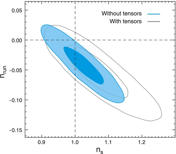
Figure 11. Two-dimensional marginalized limits for the spectral index, ns, defined at k0 = 0.002 Mpc−1, and the running of the index dns/dln k (marked nrun). Models with no tensor contribution, and with a tensor contribution marginalized over, are shown. In both cases the models are consistent with a power-law spectral index, with dns/dln k = 0, as expected from the simplest inflationary models.
Download figure:
Standard image High-resolution image4.1.3. Entropy Perturbations
The simplest classical single-field inflation models predict solely adiabatic fluctuations, but entropy (or isocurvature) fluctuations are also predicted in a wide range of scenarios, including axions (Seckel & Turner 1985; Linde 1985), multifield inflation (Polarski & Starobinsky 1994; Garcia-Bellido & Wands 1996; Linde & Mukhanov 1997), and decay of fields such as the curvaton (Lyth & Wands 2002; Moroi & Takahashi 2001; Bartolo & Liddle 2002; Lyth et al. 2003). They may be correlated with the adiabatic fluctuations to some degree, depending on the model. Most physical scenarios generate only CDM or baryon entropy fluctuations (Bond & Efstathiou 1987; Peebles 1987), with perturbation
for CDM with density ρc. Neutrino modes are also possible (Bucher et al. 2000). It has been known for some time that the CMB data cannot be fit by pure entropy fluctuations (Stompor et al. 1996; Langlois & Riazuelo 2000), but a contribution may be allowed. Several groups have placed limits on a variety of models using the WMAP one-year and three-year data (Peiris et al. 2003; Valiviita & Muhonen 2003; Bucher et al. 2004; Beltran et al. 2004; Dunkley et al. 2005; Kurki-Suonio et al. 2005; Lewis 2006; Bean et al. 2006; Trotta 2007; Keskitalo et al. 2007), finding no strong evidence for entropy fluctuations. Significant levels have been found to be consistent with the CMB data (Bucher et al. 2004; Moodley et al. 2004; Bean et al. 2006), but require correlated admixtures of CDM and neutrino isocurvature perturbations that are hard to motivate physically.
Here, and in Komatsu et al. (2009), we quantify the relative contributions to the angular power spectrum following Beltran et al. (2004) and Bean et al. (2006), with

summing the spectra from curvature fluctuations  , entropy fluctuations
  with power spectrum

and a cross-correlation spectrum CXℓ with power spectrum

This follows the definition of the curvature perturbation  by Komatsu et al. (2009), which gives large-scale temperature anisotropy
  . An anticorrelated spectrum with β = −1 gives a positive CXℓ on large scales.
Limits are found for α−1, corresponding to anticorrelated models with β = −1. This could correspond to a curvaton scenario in which inflation is driven by an inflaton field, but CDM perturbations are generated by the decay of a distinct curvaton field (see, e.g., Lyth & Wands 2002). In this case, we make the assumption that the spectral index of the anti-uncorrelated entropy fluctuations is equal to the adiabatic spectral index. We do not find evidence for curvaton entropy perturbations, finding a limit from the WMAP of α−1 < 0.011(95%CL), shown in Figure 12 and Table 5. This is half the three-year limit, and places strong lower limits on the possible density of the curvaton at its decay, in this scenario, compared to the total energy density (Komatsu et al. 2009). If the curvaton field dominated at its decay, the perturbations would be purely adiabatic. Where has the improvement come from? The pure entropy spectrum and the cross-correlated spectrum both add large-scale power, so a similar degeneracy is seen with the spectral index, and σ8, as in the case where the tensor amplitude is varied. The entropy spectrum is also out of phase with the adiabatic spectrum, so the improved TE measurements combine with the third-peak TT spectrum to tighten the limits.

Figure 12. Marginalized two-dimensional limits (68% and 95%) on the amplitude of possible CDM entropy (or isocurvature) fluctuations. The one-dimensional 95% upper limits are given in the legend. Left: anticorrelated fluctuations are tightly constrained, placing limits on curvaton models. Right: uncorrelated fluctuations, corresponding to axion models for dark matter, add less power to the CMB spectrum than the anticorrelated case, for a given α, so higher values of α0 are allowed (than α−1), by the data. In both cases the amplitude is correlated with the spectral index of curvature fluctuations ns, which compensates for the large-scale power added by the CDM entropy fluctuations.
Download figure:
Standard image High-resolution imageTable 5. Subset of Cosmological Parameter Constraints for ΛCDM Models with Additional Anticorrelated (β = −1) or Uncorrelated (β = 0) Entropy Fluctuations
| Parameter | β = −1 | β = 0 |
| α−1 | <0.011(95%CL) | |
| α0 | <0.16(95%CL) | |
| ns | 0.983 ± 0.017 | 0.987 ± 0.022 |
| σ8 | 0.778+0.039−0.038 | 0.777 ± 0.038 |
Download table as: ASCIITypeset image
We also place limits on α0, corresponding to an uncorrelated model with β = 0. In this case the entropy spectral index is set to be scale invariant. Komatsu et al. (2009) describe how this corresponds to entropy perturbations created by axions, which would constitute some part of the dark matter budget. The limit is α0 < 0.16(95%CL), 10 times higher than the anticorrelated amplitude, but still preferring pure adiabatic fluctuations. Without the large-scale power contribution from the anticorrelated spectrum, a much larger amplitude is permitted, but with the same degeneracy with the spectral index and σ8. This has implications for the maximum deviation from adiabaticity of axion dark matter and photons. Komatsu et al. (2009) provide a discussion of the theoretical implications of these limits, and those for combined data, for both models considered.
4.2. Composition and Geometry of the Universe
4.2.1. Number of Relativistic Species
Neutrinos are expected to play an important role in the dynamics of the early universe. For standard parameters, they contribute about 40% of the energy density of the universe during the radiation epoch and about 11% of the energy density of the universe at z ∼ 1100 (very close to the energy density in baryons). Because neutrinos contribute to the expansion of the universe and stream relativistically out of density fluctuations, they produce a significant imprint on the growth rate of structure and on the structure of the microwave background fluctuations (e.g., Ma & Bertschinger 1995). The amplitude of these effects depend upon Neff, the number of effective neutrino species. By "effective neutrinos species," we are counting any particle that is relativistic at z ∼ 1000–3000, couples very weakly to the baryon–electron–photon fluid, and has very weak self-interactions. Because we know neutrinos exist, we associate "neutrinos" with "light relativistic particle," but note that in the strictest sense we limit only light relativistic species, as the cosmological constraints are sensitive to the existence of any light species produced during the big bang or any additional contribution to the energy density of the universe (e.g., primordial magnetic fields).
Measurements of the width of z provide very tight limits on the number of neutrino species: Nν = 2.984 ± 0.008 (Particle Data Book), consistent with the three light neutrino species in the standard model. Because of nonthermal effects due to the partial heating of neutrinos during the e± annihilations, and other small corrections, the effective number of species is 3.0395 (Dicus et al. 1982; Mangano et al. 2002). Most analyses of the number of neutrino species with three-year WMAP data (Spergel et al. 2007; Ichikawa et al. 2008; Mangano et al. 2007; Hamann et al. 2007; de Bernardis et al. 2008) relied on combining CMB measurements with probes of the growth rate of structure. Since one of the signatures of the number of neutrino species is a change in the growth rate of structure, there are degeneracies between the properties of the neutrinos and of the dark energy. Neutrinos, however, leave a distinctive signature directly on the CMB power spectrum (see Bashinsky & Seljak 2004 for detailed discussion): the neutrinos not only suppress the CMB peak heights, they also shift the acoustic peak positions. While the effects that depend on shifts in the epoch of matter/radiation equality are degenerate with changes in the matter density, the effects of neutrino free streaming are distinct. Changes in the baryon/matter ratio and the baryon/photon ratio also have their own imprints on the Silk damping scale and on the acoustic scale. With five years of data, we are now able to see evidence of the effects of the neutrinos on the CMB power spectrum.
Figure 13 shows the limits on the number density of neutrinos and the density in dark matter. The degeneracy valley, shown in the right panel, corresponds to a constant ratio of matter density to radiation density, or equivalently a measurement of the expansion factor at matter radiation equality:
With only three years of data and a lack of precision on the third peak position and height, WMAP was not able to make a clear detection of neutrinos (or relativistic species); however, the data did provide a ∼2σ hint of the effects of neutrino anisotropic stresses (Melchiorri & Serra 2006). Figure 13 shows that with the five-year data alone we now constrain the number density of relativistic species: Neff > 2.3(95%CL). By bounding Neff < 10, and choosing a uniform prior on Neff, this level of significance depends somewhat on the prior. We therefore test the significance of the constraint by comparing two ΛCDM models: one with Neff = 0, and one with the standard Neff = 3.04. We find that the data prefer Neff = 3.04. The best-fit model has Δ(−2ln L) = 8.2 less than the Neff = 0 best-fit model, corresponding to evidence for relativistic species at >99.5% confidence. The CMB power spectra corresponding to these two models, and their fractional difference, are shown in Figure 14. The model with no neutrinos has a lower matter density, Ωmh2, in order to keep zeq fixed. The improvement in likelihood between the two models comes from both the low-ℓ and high-ℓ TT spectrum, with a small contribution from the TE spectrum. We also check that this evidence does not go away if we relax the assumption of a power-law spectral index, by testing a model with a variable running, dns/dln k ≠ 0.

Figure 13. Evidence for a nonzero effective number of neutrino species, Neff. Left: the marginalized probability distribution gives Neff > 2.3(95%CL) from WMAP alone. The best-fit ΛCDM model with Neff = 0 is a poorer fit to the data than Neff = 3, with Δχ2 = 8.2. Inferred 95% limits from BBN observations are highlighted. Right: joint two-dimensional distribution for Neff and the CDM density, Ωch2, with five-year limits in blue, compared to three-year limits in gray. The degeneracy valley of constant zeq is shown dashed, indicating that the CMB is now sensitive to the effect of neutrino anisotropic stress, which breaks the degeneracy.
Download figure:
Standard image High-resolution image
Figure 14. Comparison of the CMB angular power spectrum for the best-fit ΛCDM models with the standard Neff = 3.04 neutrino species (red), and with Neff = 0 species (blue). The lower panel shows the fractional difference between the two spectra when Neff is increased from 0 to 3.04. The Neff = 0 model has a lower Ωmh2 in order to fit the third peak, and a lower spectral index, ns, compared to the Neff = 3.04 model.
Download figure:
Standard image High-resolution imageKomatsu et al. (2009) combine WMAP data with other distance indicators (which constrain Ωch2) and finds a stronger limit on the number density of neutrino species: Neff = 4.4 ± 1.5. These limits will continue to improve as CMB measurements of the higher peaks improve. The CMB constraints on the number of relativistic species at redshift ∼1000–3000 complement constraints from BBN and from particle accelerators. Measurements of the abundance of helium are sensitive to the expansion rate of the universe during its first few minutes (Steigman et al. 1977). The agreement between the best-fit value from BBN, Neff = 3.24 ± 1.2 (95% confidence interval; Cyburt et al. 2005; Particle Data Book 2007), with the best-fit CMB value is another consistency check for standard cosmology.
4.2.2. Neutrino Mass
Cosmological data places limits on the mass of neutrinos. Atmospheric and solar neutrino experiments show that neutrinos are massive (see Mohapatra et al. 2007), and measure the difference between the square of their masses, m2νi − m2νj. Cosmological measurements constrain the sum of the masses ∑mν due to their effect on the propagation of perturbations, on the clustering of matter, and on the expansion rate of the universe (Bond & Szalay 1983; Ma 1996; Hu et al. 1998). The mass has a large effect on the matter power spectrum, as massive neutrinos do not cluster as well as cold dark matter, leading to a suppression in power on small scales. Neutrinos also affect the CMB at earlier times: if the fraction of dark matter that is warm is raised, acoustic oscillations in the photon–baryon plasma are less strongly damped for modes that entered the horizon while the neutrinos were relativistic, raising the acoustic peak amplitudes. The radiationlike behavior at early times also changes the expansion rate, shifting the peak positions.
These effects are somewhat degenerate with other parameters, so CMB data alone cannot limit the mass as well as when combined with other data. With the three-year WMAP data alone the limits were ∑mν < 1.8 eV (Spergel et al. 2007), and <0.66 eV when combined with other data. Since the three-year WMAP analysis there have been many studies of the constraints, as discussed by Komatsu et al. (2009).
The five-year WMAP data now give an upper limit on the total mass to be ∑mν < 1.3 eV(95%CL), as shown in Table 6. We have checked that this upper limit is robust to the choice of cosmological models. The upper limit is raised by <10% when we include tensor fluctuations, a running spectral index, or a constant w ≠ −1 equation of state of dark energy, as shown in Figure 15. This dependence on additional parameters is consistent with earlier investigations by, e.g., Crotty et al. (2004) and Zunckel & Ferreira (2007). A larger neutrino mass raises the amplitude of the higher acoustic peaks, hence the observed degeneracy with σ8 (Figure 15). Stronger constraints come from combining the CMB data with probes of the expansion rate and clustering of matter at later times: Komatsu et al. (2009) find ∑mν < 0.61(95%CL) for WMAP combined with additional data.
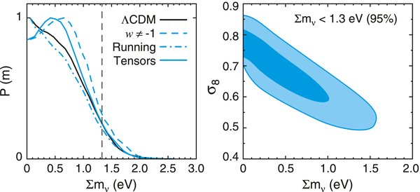
Figure 15. Limits on the sum of neutrino masses with the WMAP five-year data. Left: marginalized one-dimensional limit from WMAP alone is ∑mν < 1.3 eV(95%CL). This is raised by <10% with marginalization over a running spectral index, tensor fluctuations, or a dark energy equation of state w. Right: the neutrino mass is anticorrelated with σ8, the amplitude of matter fluctuations.
Download figure:
Standard image High-resolution imageTable 6. Constraints on Neutrino Properties and the Primordial Helium Fraction
| Parameter | Limits |
|---|---|
| Neff | >2.3(95%CL) |
| ∑mν | <1.3 eV(95%CL) |
| YP | <0.45 (95% CL) |
Download table as: ASCIITypeset image
4.2.3. Primordial Helium Abundance
In most cosmological analyses the primordial helium abundance is fixed to be YP = 0.24, motivated by observations discussed in Section 3.2.9. The effect of the abundance on the CMB spectrum is small, but provides an independent cross-check of the BBN results, and probes for any difference between the helium abundance during the first few minutes, and after 300,000 years. The abundance affects the CMB at small scales due to the recombination process. The number density of electrons before recombination depends on the helium fraction through ne = nb(1 − YP), where nb is the baryon number density. Changing the electron number density changes the mean free path of Compton scattering, which affects the Silk damping scale. A larger Yp increasingly damps the power on small scales, as shown by Trotta & Hansen (2004).
Constraints from the first-year WMAP data were presented by Trotta & Hansen (2004), Huey et al. (2004), and Ichikawa & Takahashi (2006), with 99% upper limits of YP < 0.65 inferred (Trotta & Hansen 2004). A subsequent analysis of the three-year data gave YP < 0.61 at 95% confidence, tightened to 0.25 ± 0.10 with small-scale CMB data (Ichikawa et al. 2008). We now find YP < 0.45 (95% CL) with the five-year WMAP data. Higher values allowed by the three-year data are disfavored with a better measure of the third acoustic peak height. With future small-scale CMB measurements, for example from the Planck satellite, constraints should significantly improve (Ichikawa et al. 2008; Hamann et al. 2008b).
4.2.4. Curvature of the Universe
In combination with other data, WMAP observations place strong constraints on the geometry of the universe (Spergel et al. 2007). The CMB measures with high accuracy the angular scale at which acoustic oscillations are imprinted at the last scattering surface, θ* = 0 5952 ± 00017. However, this alone does not provide a good measure of the geometry, as there is a degeneracy with the expansion rate of the universe since last scattering. This is shown in Figure 16, indicating the degeneracy between the dark energy density ΩΛ and the curvature Ωk. With WMAP alone the curvature is weakly constrained, with marginalized limits Ωk = −0.099+0.085−0.100, and ΩΛ < 0.76(95%CL), assuming a Hubble prior of 20 < H0 < 100 and ΩΛ > 0. Without this prior on the positivity of ΩΛ, limits on the curvature are weakened. The same degeneracy is seen, although slightly broadened, when the dark energy equation of state is allowed to vary. However, in both cases the Hubble constant decreases with increasingly negative curvature, taking values inconsistent with observation. This degeneracy can be used to constrain the curvature by combining observations (Jungman et al. 1996). In the three-year WMAP analysis, Spergel et al. (2007) showed that the degeneracy is truncated with the addition of only one piece of additional cosmological data (Type Ia supernovae, or the HST measurement of the Hubble constant, or galaxy power spectra), tightly constraining any deviations from flatness. Komatsu et al. (2009) draw similar conclusions with currently available data, and discuss the current limits on the spatial curvature from recent observations.
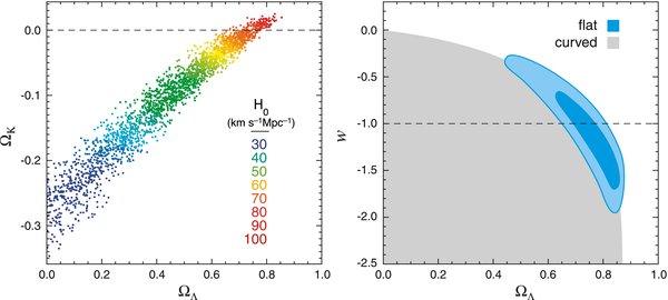
Figure 16. Left: the points show the set of nonflat models consistent with the WMAP data, colored by the Hubble constant values. WMAP measures the acoustic peak scale to high accuracy, but does not constrain the curvature, Ωk, by itself. However, the highly curved models have a low Hubble constant, inconsistent with observation. Right: constraints on the dark energy equation of state, w, and the dark energy density, ΩΛ, from WMAP alone. With a Hubble constant H0 < 100, weak limits can be placed on w in a flat universe, shown by the blue contours, but the dark energy density and equation of state are unconstrained (with the 95% CL; shaded gray) if the assumption of flatness is relaxed. Limits are significantly improved when WMAP is combined with additional data (Komatsu et al. 2009).
Download figure:
Standard image High-resolution image4.2.5. Dark Energy Properties
The ΛCDM model requires a nonzero dark energy density ΩΛ = 0.742 ± 0.030 to fit the data, which is assumed to be in the form of a cosmological constant. We do not have an explanation for this component of the universe. A natural explanation could be a vacuum energy density (Carroll et al. 1992), but if so, we are faced with the fine-tuning problem to explain its observed value, 120 orders of magnitude smaller than expected from field theory arguments. Alternative explanations include quintessence (Peebles & Ratra 1988; Wetterich 1988; Ferreira & Joyce 1998) or modifications to gravity (Deffayet et al. 2002). Testing the dark energy equation of state today, and as a function of cosmic time will help identify the possible explanation.
The CMB by itself cannot place strong limits on the equation of state w = p/ρ, but by measuring the acoustic peak positions and heights, and constraining Ωmh2 with the third peak, limits the range of models to a degeneracy between Ωm and w, as shown in Figure 16. The dark energy in these models is allowed to cluster. With a prior on the Hubble constant H0 < 100, WMAP alone places weak limits w = −1.06+0.41−0.42, with ΩΛ = 0.73+0.10−0.11. If flatness is not assumed, the WMAP data cannot constrain w or ΩΛ due to the geometric degeneracy, also shown in Figure 16. However, the situation is significantly improved when WMAP is combined with astronomical data measuring the expansion rate and clustering of matter at late times. Komatsu et al. (2009) discuss limits obtained from various data in combination with WMAP, and find w constrained to be −1 to within 6% for a flat universe and constant equation of state.
5. CONCLUSIONS
The simple six-parameter ΛCDM model continues to fit the WMAP data. With five years of observations, we have better measured both the temperature and polarization anisotropy of the CMB. This has allowed us to measure with smaller errors, compared to the three-year analysis, the third acoustic peak in the temperature spectrum, and the low-ℓ polarization signal, leading to improved constraints on the cosmological parameters describing the contents of the universe, and the primordial fluctuations that seeded structure. The observations continue to be well fit by the predictions of the simplest inflationary models, with a scale-invariant spectrum of fluctuations disfavored. Consistency with the TE cross-correlation spectrum, now measured with better accuracy, provides additional confidence in this simple model.
We have detected the optical depth to reionization with high significance. This measurement implies that reionization of the universe likely took place gradually, as it constrains a sudden reionization to be earlier than consistent with other observations. With more data, it will become possible to use the polarization data to better quantify the ionization history. Given the improvement in this measurement, and with a view to interpreting future large-scale polarization measurements, we develop an alternative way to remove Galactic foregrounds from low-resolution polarization maps, which includes marginalization over uncertainties in the Galactic signal. We find consistent results using this method and the standard template-cleaning method.
Considering a range of extended models, we continue to find that the standard ΛCDM model is consistently preferred by the data. The improved measurement of the third peak now requires the existence of light relativistic species, assumed to be neutrinos, at high confidence. The standard scenario has three neutrino species, but the three-year WMAP data could not rule out models with none. The ΛCDM model also continues to succeed in fitting a substantial array of other observations. Certain tensions between other observations and those of WMAP, such as the amplitude of matter fluctuations measured by weak lensing surveys and using the Lyα forest, and the primordial lithium abundance, have either been resolved with improved understanding of systematics, or show some promise of being explained by recent observations. With further WMAP observations we will better probe both the universe at a range of epochs, measuring fluctuation characteristics to probe the initial inflationary process, or other non-inflationary scenario, improving measurements of the composition of the universe at the recombination era, and characterizing the reionization process in the universe.
The WMAP mission is made possible by the support of the Science Mission Directorate Office at NASA Headquarters. This research was additionally supported by NASA grants NNG05GE76G, NNX07AL75G S01, LTSA03-000-0090, ATPNNG04GK55G, and ADP03-0000-092. E.K. acknowledges support from an Alfred P. Sloan Research Fellowship. We thank Antony Lewis for discussion about lensing in CAMB, Will Percival for discussion and provision of BAO data, Catherine Heymans, Jonathan Benjamin, and Richard Massey for discussion of weak lensing data, Michael Wood-Vasey for discussion of ESSENCE supernova data, Eric Aubourg for discussion of SNLS supernova data, Gary Steigman for discussion of BBN constraints, Bruce Draine and Todd Thompson for discussion of dust and synchrotron emission. This research has made use of NASA's Astrophysics Data System Bibliographic Services. We acknowledge the use of the HEALPix, CAMB, CMBFAST, and CosmoMC packages.
APPENDIX A: LOW-ℓ TT LIKELIHOOD CROSS CHECKS
We have switched from the pixel likelihood to a Blackwell–Rao (BR) estimator at low-ℓ, so we perform several tests to verify that the new likelihood (1) is consistent with the pixel likelihood, (2) is insensitive to several choices of input data, and (3) is properly converged. Many of our checks involve comparing likelihoods. Because the likelihood is a function on a high-dimensional space, we do not check it everywhere. Instead we choose some fiducial spectrum and compute slices through the likelihood. We compare these conditional likelihoods, typically in the form of maximum likelihood values and full-width-half-maximum error bars between different low-ℓ likelihood methods. We also compare ΛCDM cosmological parameters obtained using different inputs.
The first comparison is between the pixel-based code and the Gibbs code. Figure 1 showed a comparison of the Cℓ likelihoods, with no significant differences, even though they use different resolutions. The cosmological parameters are unchanged for the two codes. The next comparison is between likelihoods from Gibbs sampling at two different resolutions, Nside = 16 and 32. Table 7 lists details of runs at these two different resolutions, including the standard deviation of the Gaussian white noise added to the smoothed maps. The power spectrum of the white noise for the Nside = 32 case, is compared to the input noise and cosmic variance in Figure 17. Power spectra are sampled up to ℓmax (sampled), and the sampled CMB skies are constructed with the sampled power spectra and by conditioning on a constant fiducial spectrum out to a higher value of ℓmax (conditioned). In Figure 18 the estimated spectra are compared, using the fiducial KQ85 mask. There are some small differences, but the spectra are consistent.

Figure 17. Angular power spectra of signal and noise components in the smoothed ILC map used for Gibbs sampling the low-ℓ temperature spectrum. Uncorrelated noise, at 2 μK per pixel (red), is added to the smoothed ILC map to speed up the sampling, and then is assumed to be the only noise present. This assumption is inaccurate at low ℓ, as it ignores the true noise (blue), but the error is negligible since it is significantly lower than cosmic variance (green).
Download figure:
Standard image High-resolution image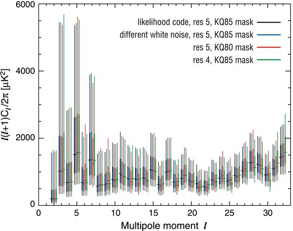
Figure 18. Level of variation in the low-ℓ TT Gibbs likelihood that arises from different input parameters. The spectrum estimated from the standard input (black) is compared to results obtained using a different white noise realization (blue), using a larger mask (KQ80, red), and degrading to Nside = 16 (green) rather than 32. The likelihood does fluctuate with these changes, but has a negligible effect on cosmological parameters. The values shown at each multipole correspond to maximum likelihood values obtained by fixing the spectrum of other multipoles at fiducial values. The error bars show where the likelihood is at 50% and 5% of its peak value.
Download figure:
Standard image High-resolution image
Table 7. Parameters Used for Sampling the Low-ℓ TT Likelihood at Two Different Resolutions
| Resolution parameter | 4 | 5 |
| Smoothing FWHM | 91831 |
50 |
| σnoise/pixel (μK) | 1.0 | 2.0 |
| ℓmax sampled | 32 | 51 |
| ℓmax conditioned | 48 | 96 |
Download table as: ASCIITypeset image
We also show in Figure 18 that the spectra obtained are almost identical for two different realizations for the added uncorrelated white noise, and that using the larger KQ80 mask, compared to the fiducial KQ85, has a small effect on the spectra and cosmological parameters, consistent with noise. Finally, we compare results for different ℓmax used in the BR estimator. The standard set-up uses ℓmax = 32; using the low-ℓ likelihood up to ℓ = 51 has almost no effect on cosmological parameters.
APPENDIX B: PARAMETER ESTIMATION DETAILS
B1. Sampling Method
In the primary pipeline, only one chain is run for each model, rather than the typical four or eight parallel chains used in most MCMC cosmological analyses. This is possible as our spectral convergence test only requires a single chain. The starting points are picked as good-fitting points from previous analyses (e.g., a good-fitting value from the three-year WMAP analysis), or previous test chains, which means that no initial burn-in need be removed. Starting afresh with the five-year data, one can always use a point lying in the WMAP three-year limits as a starting point. This would not be the case for entirely new distributions, or much improved data, in which case we run a short initial exploratory chain to find the high-likelihood region.
The covariance matrix from which trial steps are drawn, is chosen using a best guess for the covariance C of the distribution being sampled. For a multivariate Gaussian with covariance C, the optimal trial covariance matrix, if all parameters are sampled simultaneously, is CT = (σT/σ0)2C, where
for D-dimensional distributions (Gelman et al. 1996; Hanson & Cunningham 1998; Dunkley et al. 2005). This relation also holds for somewhat non-Gaussian distributions. At each step we draw a vector G of D Gaussian unit variance zero mean random variates, and compute a trial set of parameters xT, starting from the current position xi, where

Using an appropriate covariance matrix can speed up the sampling time by a factor of hundreds. In practice, we have a good idea of the covariance from previous cosmological analyses, so this is always used as a starting point. With significantly different data, or with new parameters, a best guess is made. The chains are then run for a few thousand steps, and then updated if the matrix is inadequate. This is determined by the acceptance rate of the chain, which should be ∼15%–25% and by the chain efficiency, using the spectral test described in the following section. A second or third update may be required for models such as those with curved geometries with variable dark energy equation of state. Once a good covariance matrix is found, the chains are run for typically 20,000 steps, and then tested for convergence. Convergence for ΛCDM chains typically takes place after only ∼ 6000 iterations, although at this point the 1D and 2D distributions are noisy. In practice, we then run all the chains for longer than the convergence limit, typically for 100,000 iterations, in order to get well-sampled histograms. The chains are not thinned before analysis.
B2. Spectral Convergence Test
A chain has "converged" when its statistical properties reflect those of the underlying distribution with sufficient accuracy. To determine this stopping point, we use the spectral convergence test described by Dunkley et al. (2005) in our main parameter pipeline. The power spectrum of each parameter of the chain is used as a diagnostic, to check whether the chain has (1) sampled the distribution in such a way that it is unbiased by correlations and (2) sampled enough points that statistics can be estimated with sufficient accuracy. The Gelman & Rubin test (Gelman & Rubin 1992), commonly used in cosmology, can sometimes fail to test the first point, producing a false positive.
To estimate the power spectrum P(k) from a chain of length N we construct  , where j = 2πk/N, by taking the discrete Fourier Transform of the chain of values for each parameter, x,
where −(N/2 − 1) < j < N/2. x(n) is the value at each iteration n, so chains stored in weighted format are converted to unweighted arrays for analysis. Since the Metropolis algorithm produces chains which are correlated on small scales, the power spectrum tends to a white noise spectrum on large scales, and turns over to a spectrum with suppressed power at large k, with the turnover position reflecting the inverse correlation length. In Dunkley et al. (2005) it is shown that the spectrum can be fit by the following template:
with P0 giving the amplitude of the white noise spectrum in the k → 0 limit. k* indicates the position of the turnover to a different power-law behavior, characterized by α, at large k. This model is shown in Figure 3 of Dunkley et al. (2005), fitting the noisy spectrum of a parameter from a chain. The model fits the noise-averaged spectrum of a real chain obtained from Monte Carlo simulations, also shown in Dunkley et al. (2005).
To fit the parameters ln P0, k* and α to  using least squares for a finite chain, we have
where γ = 0.577216 is the Euler–Mascheroni constant, and rj are random measurement errors. The parameters are fit over the range of Fourier modes 1 ⩽ j ⩽ 10j*, for a spectrum with j* = k*(N/2π), so we iterate twice to converge on the j* limit.
For convergence, the largest scales probed must be in the white noise regime P(k) ∼ k0, defined by the requirement j*>20 for each parameter. This ensures that the correlated points are not biasing the distribution and indicates that the chain is drawing points throughout the full region of high probability. To test sufficient accuracy, we require the convergence ratio  to be less than 1% for each parameter, where
  is the variance in the sample mean, and σ20 is the variance of the sampled parameter. The Gelman & Rubin test incorporates a similar ratio: their R-statistic roughly translates to R ∼ 1 + r, but the quantity is calculated using multiple parallel chains. It is shown in Dunkley et al. (2005) that r can be estimated using a single chain, since estimating the sample mean variance of a long chain, with zero mean, is equivalent to estimating P(k) at k = 0:
In practice, we rescale each parameter to have zero mean and unit variance before computing its power spectrum. Then we estimate the value of P0 for each parameter, to compute r = P0/N. We require r < 0.01, but in practice obtain much smaller values, typically with r < 0.001.
Footnotes
- *
WMAP is the result of a partnership between Princeton University and NASA's Goddard Space Flight Center. Scientific guidance is provided by the WMAP Science Team.
- 15
The number of pixels is 12N2side, where Nside = 23 for resolution 3 (Gorski et al. 2005).
- 16
We use the pre-2008 March version of CAMB that treats reionization as "instantaneous" (with width z ∼ 0.5) and fully ionizes hydrogen but not helium at reionization.