


ABSTRACT
The AGN and Galaxy Evolution Survey (AGES) is a redshift survey covering, in its standard fields, 7.7 deg2 of the Boötes field of the NOAO Deep Wide-Field Survey. The final sample consists of 23,745 redshifts. There are well-defined galaxy samples in 10 bands (the BW, R, I, J, K, IRAC 3.6, 4.5, 5.8, and 8.0 μm, and MIPS 24 μm bands) to a limiting magnitude of I < 20 mag for spectroscopy. For these galaxies, we obtained 18,163 redshifts from a sample of 35,200 galaxies, where random sparse sampling was used to define statistically complete sub-samples in all 10 photometric bands. The median galaxy redshift is 0.31, and 90% of the redshifts are in the range 0.085 < z < 0.66. Active galactic nuclei (AGNs) were selected as radio, X-ray, IRAC mid-IR, and MIPS 24 μm sources to fainter limiting magnitudes (I < 22.5 mag for point sources). Redshifts were obtained for 4764 quasars and galaxies with AGN signatures, with 2926, 1718, 605, 119, and 13 above redshifts of 0.5, 1, 2, 3, and 4, respectively. We detail all the AGES selection procedures and present the complete spectroscopic redshift catalogs and spectral energy distribution decompositions. Photometric redshift estimates are provided for all sources in the AGES samples.
Export citation and abstract BibTeX RIS
1. INTRODUCTION
Surveys are a critical tool for understanding the evolution of galaxies and active galactic nuclei (AGNs). Because their properties are diverse and changing, we utilize large statistical samples of galaxies to measure the distribution of their properties and to trace the evolution of these distributions. Achieving a suitably high level of detail requires a combination of multiwavelength imaging and spectroscopy. Without a redshift estimate, one cannot infer luminosity, color, or environmental density, all quantities known to be of central importance in the behavior of galaxies and AGNs. While photometric redshifts can be used in the absence of spectroscopy, they have more systematic uncertainties (e.g., Hildebrandt et al. 2010) and have difficulty with AGNs (e.g., Brodwin et al. 2006; Rowan-Robinson et al. 2008; Assef et al. 2010). Moreover, the story of galaxy evolution involves many wavelengths of light: UV and far-IR for young stars, optical and near-IR for older stars, and X-ray, radio, and mid-IR for nuclear activity.
Decades of surveys have quantified the luminosity, color, surface brightness, star formation, and nuclear activity of low-redshift galaxies and correlated these properties with environment. The combination of the CfA Redshift Survey (de Lapparent et al. 1986) and the Palomar Sky Survey (POSS-II; Reid et al. 1991) defined the state of the art for local galaxies in the 1980's. This was followed by the Las Campanas Redshift Survey and its drift-scan CCD imaging (Shectman et al. 1996), which expanded our view to larger scales. Most recently, the Two Degree Field Galaxy Redshift Survey (Colless et al. 2001) and the Sloan Digital Sky Survey (SDSS; York et al. 2000) brought the scale of spectroscopy to the million-galaxy level. Wide area digital imaging from the Two Micron All-Sky Survey (2MASS; Skrutskie et al. 2006), SDSS, Galaxy Evolution Explorer (GALEX; Martin et al. 2005), the Spitzer Space Telescope (Werner et al. 2004), and ROSAT (e.g., Voges et al. 1999) have been combined with this spectroscopy to build a detailed characterization of nearby galaxies.
Surveys at higher redshift require much deeper imaging and fainter spectroscopy. Projects such as GOODS (Giavalisco et al. 2004), DEEP-2 (e.g., Faber et al. 2007), VVDS (Le Fèvre et al. 2005), and COSMOS (Scoville et al. 2007) now aim to survey cosmologically interesting volumes at redshifts of order unity and above. Importantly, there is substantial evolution in galaxy properties. Since z ≈ 1, the star formation rate per unit comoving volume has dropped by a factor of 10 (e.g., Hopkins & Beacom 2006, and references therein), the frequency of luminous quasars (e.g., Croom et al. 2004; Richards et al. 2005, 2006) and ultra-luminous infrared galaxies have decreased by a factor of 100 (e.g., Cowie et al. 2004; Le Floc'h et al. 2005), the total mass of galaxies on the red sequence has roughly doubled (e.g., Bell et al. 2003, 2007; Faber et al. 2007), and the specific star formation rates of massive galaxies have declined faster than those for less massive galaxies (e.g., Cowie et al. 1996; Pérez-González et al. 2008; Ilbert et al. 2010). At redshifts above unity, further evolution is clear, with galaxies getting notably smaller (e.g., Daddi et al. 2005; van Dokkum et al. 2010), possibly with changing correlations of star formation with environment (e.g., Scodeggio et al. 2009; Cooper et al. 2010).
Mapping galaxy properties at intermediate redshift (z ∼ 0.5) and the demographics of AGNs at any redshift requires wider fields than these deep surveys can provide. We designed the AGN and Galaxy Evolution Survey (AGES) to address these questions, combining spectroscopy from the Hectospec instrument on the MMT (Fabricant et al. 1998; Roll et al. 1998; Fabricant et al. 2005) with superb multiwavelength imaging in the NOAO Deep Wide-Field Survey (NDWFS) Boötes field. This field contains deep imaging at optical and near-IR bands (Jannuzi & Dey 1999; Elston et al. 2006) as well as full-field coverage from Spitzer IRAC (Eisenhardt et al. 2004 and later Ashby et al. 2009) and MIPS (Soifer & Spitzer/NOAO Team 2004), Chandra (Murray et al. 2005; Kenter et al. 2005; Brand et al. 2006), GALEX (Martin et al. 2005), and radio (Becker et al. 1995; de Vries et al. 2002) facilities. As we detail below, AGES provides spectroscopic redshifts for 18,163 galaxies to I = 20 and 4764 AGN candidates to I = 22.5 in the 9 deg2 field.
AGES sought to exploit the diversity of available imaging data by a multi-faceted targeting strategy. AGNs were selected by optical color, IRAC color, and MIPS, X-ray, or radio detection. The result is a large and broad sample of AGNs, including nearly 200 deg−2 at z > 1 and nearly 400 deg−2 in total. The galaxy sample required sparse sampling to reach I = 20, but we tuned the sparse sampling algorithm to ensure full sampling of brighter magnitude thresholds in 10 different bands from the UV to the mid-IR. The AGES observational strategy returned to the field many times with rolling acceptance, with the result of very high completeness in the statistical samples. This also means that fiber collisions are an unimportant problem even in high density regions. AGES is well tuned for the study of galaxy properties at 0.2 < z < 0.6 and AGN properties out to z = 5 over a cosmologically sized volume with pan-chromatic spectral energy distributions (SEDs).
This paper presents the AGES data set and data release. Section 2 describes survey design and target selection. Section 3 discusses the observations themselves. Section 4 describes the data reduction procedures. Section 5 summarizes the resulting samples and Section 6 introduces the files of the data release. We conclude in Section 7. All magnitudes and fluxes are in the system used by the parent survey. These are Vega magnitudes for the BW, R, I, J, K, Ks, and IRAC bands,12 AB magnitudes for the FUV, NUV, and z' bands, mJy for MIPS 24 μm band and the radio observations, and 0.5–7 keV counts for the X-ray observations.
2. SURVEY DESIGN
We selected targets at all wavelengths from radio through X-ray to take full advantage of the available imaging data. We start with the optical data of the NDWFS itself in the BW, R, and I bands (Jannuzi & Dey 1999), since our ability to measure spectra is limited by the optical flux. We used the zBoötes (Cool 2007) data to help target high-redshift quasars. In the near-infrared we used the K-band data of the NDWFS and the J/Ks-band data of the FLAMEX survey (Elston et al. 2006). In the mid-infrared we used the 3.6, 4.5, 5.8, and 8.0 μm data from the IRAC Shallow Survey (Eisenhardt et al. 2004). We used the 24 μm data from Soifer & Spitzer/NOAO Team (2004). In the radio we used the Faint Images of the Radio Sky at Twenty cm (FIRST) survey (Becker et al. 1995) and the deeper 1.4 GHz Westerbork Synthesis Radio Telescope (WSRT) catalog of de Vries et al. (2002). Going to shorter wavelengths, we used data from GALEX (Martin et al. 2005) in the UV and the Chandra XBoötes survey (Murray et al. 2005; Kenter et al. 2005; Brand et al. 2006) at X-ray wavelengths.
Our general approach was to produce well-defined, magnitude-limited samples of galaxies at all the available wavelengths from 24 μm through the GALEX FUV bands, and to target AGNs using a broad range of selection methods to a somewhat deeper optical flux limit. The galaxy samples were generally designed to be complete to an intermediate magnitude limit and then randomly sparse sampled from this intermediate limit to the overall magnitude limit. The sample definitions changed several times, with the largest change being a shift from preliminary photometric catalogs and R-band magnitude limits to revised catalogs and I-band magnitude limits between the 2004 and 2005 observing seasons.
Sparse sampling was an essential component of our strategy for studying galaxies because it was the only means of covering such a wide area to the desired depth (I < 20 mag) in reasonable time. To begin with, sparse sampling over a wider area produces samples with less cosmic variance than complete samples in smaller areas surveying smaller cosmological volumes. It also allows us to sample galaxies with very different properties with a well-defined statistical approach. In particular, by making the survey complete for bright objects and sparse sampling across many different photometric bands for fainter objects, we have a final sample with less shot noise for bright objects and the relatively rarer objects with extreme colors in any band. While the approach is more complex than previous redshift surveys, it is nonetheless straight forward to construct a complete statistical sample by weighting each object by the inverse of its sampling fraction. We provide explicit instructions on the appropriate procedures in Section 6.
In Sections 2.1, 2.2, and 2.3 we define nomenclature, outline our approach to random sparse sampling, and define the standard AGES sub-fields. In Sections 2.4, 2.5, and 2.6 we outline the sample definitions used in 2004, 2005, and 2006/2007. Samples defined in the previous years continued to be observed at the same priorities in the later years. The biggest differences were between 2004 and the later years, where we (1) shifted from an R-band-limited sample in 2004 to an I-band-limited sample, (2) shifted from preliminary NDWFS and IRAC Shallow Survey catalogs to later versions, and (3) added mid-IR quasar selection. The main differences from 2005 to 2006/2007 were to add sub-samples further exploring mid-IR quasar selection and to include the zBoötes data as a tool for AGN selection. There are many other small differences that are detailed in each subsection. We provide the selection codes for all seasons, so that it is clear why any source may have been targeted, but in the data tables we only provide the photometric information for the updated catalogs used from 2005 onwards. The photometric data are only a limited representation of the underlying catalogs—the original survey catalogs should be consulted to obtain the complete data. In each season we targeted at low priority some objects that were not part of the primary AGES project as experiments from collaborators. We very briefly outline these experiments and include their selection codes but provide no details.
2.1. Common Definitions
We will refer to the survey bands as X, FUV, NUV, BW, R, I, z', J, K, [3.6]i, [4.5]i, [5.8]i, [8.0]i, [24], FIRST, and WSRT. For the X-ray sources, X is the X-ray counts from the XBoötes survey. For the ultraviolet sources, FUV and NUV are the two GALEX filters. For the optical and near-IR, BW, R, I, z', J, and K are the SExtractor Kron-like (mag_auto) magnitudes. The K refers to both the NDWFS K/Ks and the FLAMEX Ks data. The final NDWFS magnitudes are from DR3 (http://www.noao.edu/noao/noaodeep/DR3/dr3-data.html). For the IRAC data, [3.6]i–[8.0]i are the 3.6, 4.5, 5.8, and 8.0 μm SExtractor Kron-like magnitudes where the subscript i = [3.6]–[8.0] defines the IRAC band used to define the extraction apertures. The 24 μm flux [24] is the DAOPHOT PSF-fit flux of the source. FIRST and WSRT both measured 1.4 GHz radio continuum fluxes. Where we are using the flux in a fixed aperture, we add the aperture diameter to the magnitude, so [3.6][3.6](6 0) represents the IRAC 3.6 μm flux in a 60 diameter aperture whose position was determined from the 3.6 μm image. These IRAC aperture magnitudes are, however, corrected for the extension of the IRAC point spread function beyond the aperture.
For the optical data we homogenized several aperture magnitudes for seeing variations. For each field, we took stars in the magnitude range 19 < I < 20 and computed the mean differences between the Kron-like I magnitude, presumed to be seeing independent, and the 10, 30, and 60 aperture magnitudes. These differences, which show the expected pattern of being significant for the 10 apertures and negligible of the 60 apertures, were then applied to these three aperture magnitudes for the BW, R, and I bands.
Point sources (pntsrc = 1) were defined based on the SExtractor stellarity indices of the sources in the optical (BW, R, I, and z' bands). For each target we assigned a code (bgood, rgood, igood, zgood = 1) for whether the data in each band on that target were acceptable. We flagged objects as either quasar candidates (qso = 1), galaxies (galaxy = 1), or in the later seasons AGN-galaxy (agngalaxy = 1) targets. Quasar candidates are point sources brighter than the (optical) magnitude limit for targeting quasars, galaxies are extended sources brighter than the magnitude limit for targeting galaxies, and "AGN galaxies" are extended AGN candidates brighter than the magnitude limit for targeting quasars but fainter than that for galaxies. In general, our sources are much brighter than the NDWFS survey limits, so there are few issues with star/galaxy separation.
2.2. Sparse Sampling Codes
For many of our samples we observed all targets to an intermediate magnitude limit and then randomly sparse sampled the sources between the intermediate limit and the overall flux limit of the sample. All sources were assigned a random integer code 0 ⩽ rcode < 20 dividing the sources into 20 random sub-samples each containing 5% of the targets. Once assigned to a source, these codes were preserved in all future samples. The sparse sampling fraction was then determined by the limit on the rcode used to define the sample. For objects that were not included in any of the primary samples, we assigned lower rcode values higher observing priorities than higher rcode values. This increases the completeness of the observations for the lower rcode targets, so that any decision to move to a higher sparse sampling fraction than used initially requires observations of fewer targets while ensuring that the fibers stay filled.
Figure 1 illustrates how this works for the IRAC [3.6] sample in 2006/2007 (see below). All galaxies must have I < 20 mag, so no fainter objects were targeted unless they appeared in one of the AGN samples. At I band, all galaxies were targeted if they were brighter than I < 18.5 mag, and a randomly selected 20% (rcode ⩽ 3) were targeted between 18.5 < I < 20. For the IRAC [3.6] band, galaxies were all targeted if brighter than [3.6] < 15.2 mag, and a randomly selected 30% (rcode ⩽ 5) were targeted between 15.2 < [3.6] < 15.7, but still subject to the I < 20 mag limit. Combining these criterion, all sources to the left or below the heavy solid line, 30% of the sources in the box 18.5 < I < 20 and 15.2 < [3.6] < 15.7, and 20% of the sources with 18.5 < I < 20 and [3.6] > 15.7 mag were targeted by these criterion. Between the different color weightings of the bands and the filling of fibers that could not be allocated to the primary samples, the actual fractions of sources with redshift measurements in the sparse sampling regions are much higher than 20% or 30%.
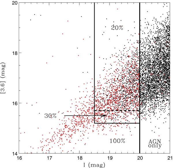
Figure 1. Distribution of galaxies in I-band and IRAC [3.6] magnitudes. The points are a randomly selected 10% of the sources in the main survey area, where red points have measured redshifts. The boundaries indicate the survey sampling regions and the sparse sampling rates. The actual fractions of redshift measurements in these regions are much higher than the nominal 20% or 30% sampling rates because of the different color weightings of the various bands and the observations of lower priority sources with unused fibers. AGNs were targeted to fainter magnitudes, leading to the redshift measurements with I > 20 mag.
Download figure:
Standard image High-resolution image2.3. Standard Fields
We defined our primary statistical samples as the union of the NDWFS field geometry with a set of 15 sub-fields defined by the Hectospec field of view. Sources had to lie within 0.49 deg of one of the 15 field centers illustrated in Figure 2 and listed in Table 1. The field centers were simply defined by the final field centers used for the primary observational runs in 2004. Sources inside the standard sub-fields are assigned the field ID of the closest field center, while those outside are assigned a field ID of −1 (see Table 2). Several of the circular fields extend beyond the NDWFS area, so the actual survey area must be clipped to exclude R.A. < 228.96 deg, Decl. > 33.46 deg, and Decl. < 35.84 deg if R.A. > 216.14 deg. The total area within this region is 2.40 × 10⁻³ sr (7.88 deg2). We also do not target sources within radius Rbstar/2 of a bright RUSNO < 17 mag USNO star, where Rbstar = 200 + 50(15 − RUSNO). For Rbstar/2 < R < Rbstar, there were additional surface brightness criteria for observing targets (see below). Excluding the bright star exclusion areas with R < Rbstar/2, the survey area drops to 2.36 × 10⁻³ sr (7.74 deg2).
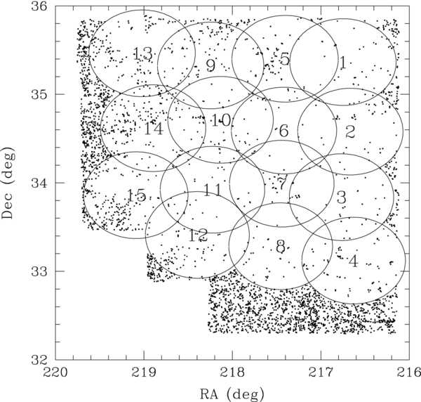
Figure 2. 15 standard sub-fields listed in Table 1. The points are the 2006/2007 primary galaxy sample targets (gcode06 neither zero nor 2048) lacking redshifts. Note the high completeness in the sub-fields and the significantly lower completeness elsewhere in the Boötes field. Some redshifts were obtained outside the standard fields because of the shifting centers of the individual Hectospec pointings.
Download figure:
Standard image High-resolution imageTable 1. The Standard Fields
| Field | R.A. | Decl. | Main Galaxy Sample | |||
|---|---|---|---|---|---|---|
| Sample | Spectra | Redshifts | Completeness | |||
| 1 | 216.750000 | 35.365000 | 774 | 772 | 753 | 97.3% |
| 2 | 216.666667 | 34.578889 | 751 | 750 | 731 | 97.3% |
| 3 | 216.766667 | 33.838333 | 729 | 723 | 710 | 97.4% |
| 4 | 216.629167 | 33.121389 | 911 | 902 | 861 | 94.5% |
| 5 | 217.404167 | 35.402500 | 688 | 667 | 633 | 92.0% |
| 6 | 217.416667 | 34.591389 | 574 | 572 | 566 | 98.6% |
| 7 | 217.441667 | 33.990833 | 551 | 546 | 529 | 96.0% |
| 8 | 217.454167 | 33.283889 | 865 | 861 | 839 | 97.0% |
| 9 | 218.245833 | 35.326667 | 652 | 631 | 602 | 92.3% |
| 10 | 218.133333 | 34.712222 | 728 | 720 | 686 | 94.2% |
| 11 | 218.225000 | 33.922500 | 614 | 612 | 603 | 98.2% |
| 12 | 218.395833 | 33.411389 | 785 | 766 | 749 | 95.4% |
| 13 | 219.020833 | 35.464167 | 786 | 717 | 697 | 88.7% |
| 14 | 218.895833 | 34.618056 | 748 | 664 | 636 | 88.8% |
| 15 | 219.091667 | 33.860833 | 855 | 737 | 711 | 83.2% |
Notes. These are the R.A./Decl. of the 15 standard sub-field centers, followed by the number of main I-band (code06 = 524288) galaxies in the field, the number for which spectra were obtained, the number of successful redshift measurements and the resulting completeness. An object is in a field if it is closer to the center than Rfld = 0.49 deg. Objects in overlapping fields are assigned to the closest field center, and objects in none of these standard sub-fields are given field number −1. See Figure 2 for the positions of the fields on the sky.
Download table as: ASCIITypeset image
Table 2. The Spectroscopic Observations
| Pass | Field | Date | R.A. | Decl. | Nexp | Texp | Nspec | Air | Mean | Comments |
|---|---|---|---|---|---|---|---|---|---|---|
| (s) | Mass | S/N | ||||||||
| 0 | 0 | Spectra from the SDSS Survey | 2946 | |||||||
| 101 | 1 | 2004.0415 | 14:26:49.36 | 35:22:05.57 | 4 | 2400 | 268 | 1.03 | 16.21 | |
| 102 | 2 | 2004.0421 | 14:26:58.80 | 34:38:07.68 | 2 | 1800 | 266 | 1.01 | 11.21 | |
| 103 | 3 | 2004.0416 | 14:26:33.20 | 33:59:51.36 | 3 | 2700 | 263 | 1.02 | 16.51 | |
| 104 | 4 | 2004.0416 | 14:26:29.20 | 33:09:53.04 | 4 | 3600 | 267 | 1.19 | 14.92 | Major ADC |
| 105 | 5 | 2004.0420 | 14:29:47.89 | 35:28:48.00 | 2 | 1440 | 262 | 1.12 | 7.09 | |
| 106 | 6 | 2004.0414 | 14:31:49.76 | 34:50:47.40 | 3 | 2700 | 267 | 1.18 | 7.66 | Not fluxed |
| 107 | 7 | 2004.0420 | 14:29:41.89 | 33:53:09.36 | 2 | 1440 | 260 | 1.03 | 10.08 | |
| 108 | 8 | 2004.0422 | 14:29:37.09 | 33:13:53.04 | 2 | 1440 | 264 | 1.00 | 11.02 | |
| 109 | 9 | 2004.0420 | 14:32:38.18 | 35:23:05.99 | 2 | 1440 | 259 | 1.06 | 7.65 | |
| 110 | 10 | 2004.0414 | 14:31:49.76 | 34:50:47.40 | 3 | 2700 | 267 | 1.04 | 8.98 | Not fluxed |
| 111 | 11 | 2004.0416 | 14:32:40.98 | 33:53:51.37 | 3 | 2700 | 263 | 1.02 | 18.17 | |
| 112 | 12 | 2004.0420 | 14:33:35.78 | 33:22:35.04 | 2 | 1440 | 268 | 1.01 | 10.06 | |
| 113 | 13 | 2004.0416 | 14:35:32.87 | 35:24:48.00 | 3 | 2700 | 258 | 1.20 | 14.22 | Major ADC |
| 114 | 14 | 2004.0421 | 14:35:36.87 | 34:39:37.68 | 2 | 1440 | 270 | 1.01 | 8.53 | |
| 115 | 15 | 2004.0420 | 14:35:36.87 | 33:58:51.36 | 2 | 1440 | 270 | 1.09 | 9.74 | |
| 201 | 1 | 2004.0421 | 14:26:26.80 | 35:22:36.00 | 3 | 2700 | 259 | 1.09 | 9.00 | |
| 202 | 2 | 2004.0422 | 14:26:58.80 | 34:38:07.68 | 3 | 2700 | 258 | 1.07 | 8.00 | |
| 203 | 3 | 2004.0421 | 14:26:33.20 | 33:59:51.36 | 3 | 2700 | 259 | 1.28 | 9.03 | Major ADC |
| 204 | 4 | 2004.0421 | 14:26:43.20 | 33:08:47.04 | 3 | 2700 | 268 | 1.04 | 8.87 | |
| 205 | 5 | 2004.0422 | 14:29:25.09 | 35:20:36.00 | 3 | 2700 | 244 | 1.29 | 6.94 | Major ADC |
| 206 | 6 | 2004.0422 | 14:29:38.29 | 34:42:01.68 | 3 | 2700 | 262 | 1.10 | 10.89 | |
| 207 | 7 | 2004.0611 | 14:29:46.29 | 33:59:27.34 | 4 | 4500 | 264 | 1.08 | 10.21 | |
| 208 | 8 | 2004.0423 | 14:29:37.09 | 33:13:53.04 | 2 | 1800 | 264 | 1.32 | 5.60 | Major ADC |
| 209 | 9 | 2004.0612 | 14:32:59.18 | 35:19:36.00 | 4 | 4500 | 276 | 1.08 | 10.87 | Not fluxed |
| 210 | 10 | 2004.0422 | 14:32:39.38 | 34:40:49.68 | 3 | 2700 | 257 | 1.01 | 9.57 | |
| 211 | 11 | 2004.0423 | 14:32:42.98 | 33:54:21.36 | 3 | 2220 | 260 | 1.01 | 6.54 | |
| 212 | 12 | 2004.0423 | 14:33:35.78 | 33:22:35.04 | 3 | 2700 | 261 | 1.06 | 6.60 | |
| 213 | 13 | 2004.0420 | 14:35:45.27 | 35:28:48.00 | 3 | 2700 | 261 | −1.00 | 9.34 | Major ADC |
| 214 | 14 | 2004.0423 | 14:35:36.87 | 34:39:37.68 | 3 | 2700 | 254 | 1.11 | 5.74 | |
| 215 | 15 | 2004.0423 | 14:35:36.87 | 33:58:51.36 | 3 | 2700 | 259 | 1.01 | 7.20 | |
| 301 | 1 | 2004.0610 | 14:27:00.40 | 35:21:54.01 | 4 | 4500 | 279 | 1.18 | 10.70 | Major ADC |
| 302 | 2 | 2004.0620 | 14:26:40.40 | 34:34:43.68 | 4 | 4500 | 262 | 1.30 | 9.61 | ADC off |
| 303 | 3 | 2004.0622 | 14:27:04.00 | 33:50:18.36 | 4 | 4500 | 268 | −1.00 | 10.93 | |
| 304 | 4 | 2004.0621 | 14:26:31.00 | 33:07:17.04 | 4 | 4500 | 264 | 1.37 | 9.68 | Major ADC |
| 305 | 5 | 2004.0616 | 14:29:36.69 | 35:24:09.00 | 4 | 4500 | 272 | 1.06 | 9.33 | |
| 306 | 6 | 2004.0615 | 14:29:40.09 | 34:35:28.70 | 4 | 4500 | 265 | 1.06 | 12.24 | |
| 307 | 7 | 2004.0615 | 14:29:46.29 | 33:59:27.40 | 4 | 4500 | 263 | 1.30 | 9.53 | Major ADC |
| 308 | 8 | 2004.0621 | 14:29:49.49 | 33:17:02.04 | 4 | 4500 | 272 | 1.07 | 10.92 | |
| 309 | 9 | 2004.0616 | 14:32:59.18 | 35:19:36.00 | 4 | 4500 | 268 | 1.29 | 9.45 | Major ADC |
| 310 | 10 | 2004.0613 | 14:32:32.37 | 34:42:43.69 | 4 | 4500 | 265 | 1.04 | 11.61 | Not fluxed |
| 311 | 11 | 2004.0614 | 14:32:53.97 | 33:55:21.36 | 4 | 4500 | 266 | 1.07 | 9.04 | Not fluxed |
| 312 | 12 | 2004.0626 | 14:33:35.18 | 33:24:41.04 | 5 | 5625 | 260 | 1.03 | 6.59 | Scattered light |
| 313 | 13 | 2004.0617 | 14:36:04.86 | 35:27:50.99 | 4 | 4500 | 266 | −1.00 | 8.95 | ADC off |
| 314 | 14 | 2004.0618 | 14:35:34.87 | 34:37:04.68 | 4 | 4500 | 270 | −1.00 | 10.94 | ADC off |
| 315 | 15 | 2004.0619 | 14:36:21.86 | 33:51:39.35 | 4 | 4500 | 267 | 1.15 | 10.96 | ADC off |
| 401 | 1 | 2005.0312 | 14:26:42.00 | 35:26:39.00 | 5 | 5400 | 261 | 1.05 | 9.12 | |
| 402 | 2 | 2005.0314 | 14:26:29.99 | 34:35:59.00 | 4 | 4080 | 241 | 1.03 | 3.82 | |
| 403 | 3 | 2005.0310 | 14:26:54.00 | 33:53:18.00 | 5 | 5100 | 261 | 1.04 | 11.17 | |
| 404 | 4 | 2005.0311 | 14:26:08.00 | 33:10:02.00 | 5 | 5400 | 253 | 1.04 | 18.58 | |
| 405 | 5 | 2005.0315 | 14:29:25.00 | 35:28:54.00 | 2 | 1800 | 253 | 1.03 | 3.09 | |
| 406 | 6 | 2005.0317 | 14:29:30.00 | 34:36:13.99 | 5 | 5400 | 250 | 1.05 | 13.39 | |
| 407 | 7 | 2005.0317 | 14:29:25.00 | 33:59:56.99 | 5 | 5400 | 249 | 1.33 | 5.49 | |
| 408 | 8 | 2005.0317 | 14:29:33.60 | 33:21:38.00 | 6 | 6480 | 247 | 1.04 | 11.42 | |
| 409 | 9 | 2005.0318 | 14:32:57.60 | 35:25:27.02 | 1 | 1080 | 244 | 1.00 | 6.38 | |
| 410 | 10 | 2005.0316 | 14:32:31.00 | 34:42:44.00 | 5 | 5400 | 253 | 1.04 | 10.37 | |
| 411 | 11 | 2005.0316 | 14:33:01.39 | 33:59:08.99 | 6 | 6480 | 246 | 1.04 | 10.27 | |
| 416 | 4 | 2005.0308 | 14:26:23.99 | 32:53:20.00 | 4 | 4320 | 260 | 1.03 | 15.12 | |
| 417 | 8 | 2005.0308 | 14:29:58.00 | 33:00:17.00 | 6 | 6480 | 261 | 1.08 | 18.75 | |
| 418 | 12 | 2005.0311 | 14:33:59.00 | 33:15:41.01 | 6 | 5400 | 259 | 1.30 | 11.45 | |
| 419 | 13 | 2005.0311 | 14:36:43.00 | 35:25:00.00 | 4 | 4320 | 258 | 1.04 | 13.25 | |
| 420 | 14 | 2005.0310 | 14:36:19.20 | 34:32:01.99 | 5 | 4800 | 253 | 1.03 | 14.06 | |
| 421 | 15 | 2005.0312 | 14:36:52.20 | 33:54:17.99 | 5 | 5400 | 261 | 1.03 | 17.77 | |
| 422 | 1 | 2005.0309 | 14:27:06.00 | 35:23:23.90 | 5 | 5400 | 253 | 1.03 | 8.46 | |
| 423 | 4 | 2005.0314 | 14:26:20.99 | 33:07:01.90 | 5 | 5400 | 252 | 1.04 | 6.69 | |
| 501 | 1 | 2005.0406 | 14:26:48.34 | 35:25:45.65 | 5 | 4500 | 252 | 1.03 | 8.66 | |
| 502 | 2 | 2005.0406 | 14:26:39.39 | 34:34:54.39 | 3 | 3300 | 264 | 1.19 | 5.99 | |
| 503 | 3 | 2005.0409 | 14:26:38.90 | 33:43:36.41 | 4 | 3640 | 262 | 1.03 | 6.09 | |
| 504 | 4 | 2005.0408 | 14:26:22.44 | 33:07:01.47 | 5 | 5400 | 262 | 1.34 | 4.27 | |
| 505 | 5 | 2005.0409 | 14:30:35.16 | 35:30:22.56 | 4 | 4320 | 258 | 1.16 | 4.50 | |
| 506 | 6 | 2005.0407 | 14:30:46.60 | 34:51:20.84 | 5 | 5400 | 260 | 1.06 | 8.86 | |
| 507 | 7 | 2005.0410 | 14:30:18.65 | 34:00:55.58 | 4 | 4320 | 258 | 1.03 | 6.70 | |
| 508 | 8 | 2005.0410 | 14:30:46.73 | 33:12:25.94 | 5 | 4500 | 257 | 1.20 | 10.96 | |
| 510 | 10 | 2005.0411 | 14:32:07.71 | 34:40:38.06 | 5 | 5400 | 258 | 1.06 | 9.17 | |
| 511 | 11 | 2005.0411 | 14:33:05.26 | 34:00:44.66 | 4 | 4320 | 261 | 1.02 | 7.05 | |
| 512 | 12 | 2005.0411 | 14:33:33.74 | 33:23:28.63 | 4 | 4320 | 254 | 1.17 | 5.74 | |
| 522 | 1 | 2005.0405 | 14:26:19.24 | 35:12:59.23 | 3 | 3240 | 215 | 1.06 | 3.96 | |
| 523 | 2 | 2005.0405 | 14:26:28.60 | 34:35:57.20 | 3 | 3240 | 238 | 1.21 | 1.49 | |
| 524 | 3 | 2005.0406 | 14:26:49.00 | 33:49:38.72 | 3 | 3240 | 232 | 1.19 | 5.49 | |
| 525 | 7 | 2005.0407 | 14:29:12.19 | 34:16:33.70 | 2 | 1920 | 233 | 1.21 | 3.43 | |
| 526 | 2 | 2005.0406 | 14:26:49.79 | 34:48:52.29 | 4 | 4320 | 226 | 1.03 | 8.46 | |
| 601 | 1 | 2005.0506 | 14:26:46.00 | 35:26:22.00 | 5 | 5400 | 256 | 1.05 | 4.65 | |
| 602 | 2 | 2005.0507 | 14:26:32.00 | 34:36:44.00 | 6 | 6300 | 263 | 1.07 | 6.58 | |
| 603 | 3 | 2005.0510 | 14:26:50.00 | 33:53:03.00 | 4 | 4320 | 253 | 1.02 | 7.75 | |
| 604 | 4 | 2005.0510 | 14:26:22.00 | 33:07:01.99 | 2 | 2160 | 256 | 1.01 | 5.04 | |
| 605 | 5 | 2005.0509 | 14:29:25.00 | 35:28:54.00 | 5 | 5220 | 261 | 1.06 | 7.27 | |
| 606 | 6 | 2005.0508 | 14:29:30.00 | 34:36:13.98 | 6 | 6480 | 259 | 1.35 | 6.63 | |
| 607 | 7 | 2005.0509 | 14:29:25.00 | 33:59:56.99 | 5 | 5400 | 258 | 1.36 | 6.91 | |
| 608 | 8 | 2005.0510 | 14:29:57.60 | 33:16:10.01 | 4 | 4320 | 262 | 1.16 | 10.97 | |
| 609 | 9 | 2005.0512 | 14:32:57.59 | 35:25:27.02 | 5 | 5400 | 261 | 1.06 | 11.52 | |
| 610 | 10 | 2005.0510 | 14:32:31.00 | 34:42:44.00 | 3 | 3240 | 254 | 1.51 | 3.70 | |
| 611 | 11 | 2005.0511 | 14:33:01.39 | 33:59:08.99 | 4 | 4320 | 258 | 1.10 | 10.07 | |
| 612 | 12 | 2005.0514 | 14:33:55.00 | 33:22:44.99 | 5 | 5400 | 256 | 1.05 | 12.57 | |
| 613 | 13 | 2005.0514 | 14:36:27.00 | 35:28:20.00 | 6 | 6480 | 261 | 1.37 | 14.64 | |
| 622 | 5 | 2005.0511 | 14:29:25.00 | 35:28:54.00 | 5 | 5400 | 258 | 1.47 | 5.85 | |
| 709 | 9 | 2005.0705 | 14:33:11.90 | 35:20:39.00 | 5 | 5400 | 257 | 1.23 | 7.34 | |
| 710 | 10 | 2005.0703 | 14:33:40.35 | 34:31:42.01 | 6 | 6480 | 259 | 1.09 | 3.76 | |
| 712 | 12 | 2005.0702 | 14:33:18.70 | 33:24:50.99 | 5 | 5400 | 260 | 1.05 | 9.78 | |
| 713 | 13 | 2005.0703 | 14:36:09.99 | 35:26:29.99 | 5 | 5400 | 258 | 1.50 | 8.96 | |
| 714 | 14 | 2005.0630 | 14:35:36.37 | 34:36:27.99 | 5 | 5400 | 258 | 1.12 | 8.22 | |
| 715 | 15 | 2005.0701 | 14:36:25.15 | 33:52:09.97 | 5 | 5400 | 258 | 1.08 | 13.82 | |
| 722 | 15 | 2005.0706 | 14:36:35.40 | 33:44:30.00 | 5 | 5400 | 241 | 1.14 | 11.81 | |
| 801 | 1 | 2006.0324 | 14:26:41.60 | 35:26:38.18 | 6 | 7200 | 256 | 1.12 | 7.34 | |
| 802 | 2 | 2006.0326 | 14:26:29.99 | 34:35:59.00 | 7 | 8400 | 263 | 1.14 | 8.07 | |
| 803 | 3 | 2006.0326 | 14:26:54.00 | 33:53:17.99 | 7 | 8400 | 265 | 1.09 | 10.16 | |
| 804 | 4 | 2006.0331 | 14:26:29.56 | 33:07:10.40 | 7 | 8400 | 266 | 1.07 | 8.08 | |
| 805 | 5 | 2006.0404 | 14:29:56.92 | 35:27:17.80 | 5 | 5107 | 261 | 1.04 | 6.08 | |
| 821 | 1 | 2006.0427 | 14:26:41.61 | 35:26:38.20 | 3 | 3600 | 252 | 1.14 | 5.18 | |
| 822 | 2 | 2006.0429 | 14:26:30.00 | 34:35:59.00 | 6 | 6600 | 260 | 1.33 | 7.69 | |
| 823 | 3 | 2006.0430 | 14:26:54.00 | 33:53:18.00 | 5 | 6000 | 267 | 1.04 | 9.01 | |
| 824 | 4 | 2006.0430 | 14:26:29.56 | 33:07:10.40 | 5 | 6000 | 261 | 1.29 | 10.56 | |
| 825 | 14 | 2006.0501 | 14:35:52.01 | 34:37:31.81 | 6 | 7200 | 263 | 1.34 | 6.04 | |
| 834 | 5 | 2006.0501 | 14:29:55.77 | 35:27:17.81 | 5 | 6000 | 262 | 1.04 | 9.77 | |
| 841 | 1 | 2006.0429 | 14:26:41.61 | 35:26:38.18 | 5 | 6000 | 251 | 1.04 | 7.88 | |
| 861 | Co-added spectra | 700 | 14.24 | |||||||
| 862 | Co-added spectra | 700 | 13.66 | |||||||
| 863 | Co-added spectra | 700 | 13.77 | |||||||
| 906 | 6 | 2007.0510 | 14:29:15.42 | 34:37:34.98 | 5 | 9000 | 260 | 1.16 | 12.58 | |
| 908 | 13 | 2007.0219 | 14:36:24.00 | 35:27:05.00 | 3 | 5400 | 242 | 1.11 | 11.99 | |
| 909 | 9 | 2007.0513 | 14:32:58.13 | 35:25:27.02 | 5 | 9000 | 263 | 1.14 | 6.32 | |
| 910 | 10 | 2007.0512 | 14:32:49.54 | 34:45:25.01 | 6 | 10800 | 267 | 1.41 | 8.90 | |
| 911 | 11 | 2007.0513 | 14:32:21.67 | 33:54:24.01 | 6 | 10800 | 265 | 1.33 | 13.08 | |
| 912 | 12 | 2007.0315 | 14:33:56.00 | 33:20:45.00 | 6 | 10800 | 263 | 1.07 | 13.12 | |
| 914 | 14 | 2007.0615 | 14:35:54.43 | 34:37:10.99 | 3 | 5400 | 246 | 1.14 | 10.34 | |
| 915 | 15 | 2007.0424 | 14:35:37.63 | 34:04:47.98 | 5 | 9000 | 262 | 1.18 | 11.72 | |
| 928 | 8 | 2007.0514 | 14:29:47.93 | 33:15:55.00 | 2 | 3600 | 264 | 1.02 | 10.02 | |
| 929 | 9 | 2007.0612 | 14:32:58.13 | 35:25:27.02 | 5 | 9000 | 252 | 1.39 | 7.38 | |
| 930 | 10 | 2007.0616 | 14:32:49.54 | 34:45:25.01 | 6 | 10800 | 264 | 1.23 | 5.62 | |
| 931 | 11 | 2007.0618 | 14:32:23.69 | 33:53:23.61 | 6 | 10800 | 263 | 1.19 | 11.80 | |
| 934 | 14 | 2007.0617 | 14:35:54.43 | 34:37:10.99 | 3 | 5400 | 263 | 1.02 | 12.72 | |
| 935 | 15 | 2007.0614 | 14:35:40.04 | 34:04:29.98 | 5 | 9000 | 252 | 1.27 | 10.93 | |
| 948 | 8 | 2007.0619 | 14:29:47.45 | 33:15:49.00 | 6 | 10800 | 261 | 1.18 | 15.23 | |
| 950 | 10 | 2007.0718 | 14:32:49.54 | 34:45:25.01 | 3 | 5400 | 264 | 1.30 | 4.77 | |
Notes. For each Pass we give the closest field center from Table 1, the R.A./Decl. of the pointing, the number of exposures, and the total exposure time. Nspec is the number of object spectra, Air Mass is the air mass near the middle of the exposures, and Mean S/N is the mean signal-to-noise ratio of the object spectra.
2.4. Sample Selection Codes
Because we select objects using a very broad range of criteria, the targets are assigned binary selection codes reported as decimal numbers for compactness. For example, in the summary Table 3, we see that in the final sample there are four selection criteria for AGN candidates and 13 for galaxies. Each selection criterion is a assigned a binary number 2n ranging from 23 = 8 for WSRT radio sources to 219 = 524288 for the main I-band galaxy sample. Codes 20 = 1, 21 = 2, and 22 = 4 were used for SDSS flux calibration stars and test samples that are not included in Table 3 (see below). The overall code for a target is then the sum of all its selection codes. For example, an object with code number 96 = 32 + 64 = 25 + 26 is an AGN candidate selected both as an MIPS point source (code 32) and as an IRAC mid-IR (code 64) candidate. The first source in Table 5 has a selection code of code06 = 720896, which as a binary number is 10110000000000000000. While the binary format is visually appealing, in practice it is easier to work with the decimal representations of the selection codes. So, this source satisfied four selection criteria (the 1's), which correspond to the main I-band sample (524288), the R-band sample (131072) and the BW-band sample (65536), with 720896 = 524288 + 131072 + 65536. The simplest way to check whether a target is in a sample is to determine whether the logical AND operation (target code) && (sample code) is true or false. For example the set of objects for which (target code) &&64 is true represents the sample of IRAC-selected quasar candidates. For the final sample definition, we also defined shorter codes separating the quasar/AGN and galaxy selection codes into two numbers (see Table 3).
Table 3. Final Samples In 2007
| Sample Name | code06 | Qshort/ | F/B/R | Total | Main | Total | Main | Total | Main | Total | Main |
|---|---|---|---|---|---|---|---|---|---|---|---|
| Gshort | Sample | Spectra | Redshifts | Completeness | |||||||
| WSRT | 8 | 4 | 896 | 884 | 789 | 785 | 592 | 588 | 66% | 67% | |
| X-ray | 16 | 8 | 3751 | 3282 | 3048 | 2895 | 2424 | 2294 | 65% | 70% | |
| MIPS | 32 | 16 | 2347 | 2070 | 2125 | 1991 | 1843 | 1725 | 79% | 83% | |
| IRAC | 64 | 32 | 5458 | 4759 | 4318 | 4079 | 3174 | 2977 | 58% | 63% | |
| MIPS | 128 | 1 | 0.3/ 0.5/30% | 5284 | 4662 | 4588 | 4484 | 4510 | 4411 | 85% | 95% |
| IRAC [8.0] | 256 | 2 | 13.8/13.2/30% | 4174 | 3536 | 3645 | 3498 | 3633 | 3490 | 87% | 99% |
| IRAC [5.8] | 512 | 4 | 15.2/14.7/30% | 4771 | 4058 | 4173 | 3982 | 4110 | 3927 | 88% | 98% |
| IRAC [4.5] | 1024 | 8 | 15.7/15.2/30% | 7261 | 6215 | 6324 | 6081 | 6234 | 5999 | 87% | 98% |
| IRAC [3.6] | 2048 | 16 | 15.7/15.2/30% | 5861 | 4992 | 5095 | 4882 | 4999 | 4792 | 87% | 98% |
| GALEX FUV | 4096 | 32 | 22.0/22.5/30% | 605 | 545 | 537 | 422 | 535 | 520 | 89% | 96% |
| GALEX NUV | 8192 | 64 | 22.0/21.0/30% | 2068 | 1836 | 1838 | 1779 | 1832 | 1775 | 89% | 97% |
| K-band | 16384 | 128 | 16.5/16.0/20% | 5676 | 5399 | 5431 | 5314 | 5416 | 5302 | 96% | 98% |
| J-band | 32768 | 256 | 18.5/17.5/20% | 4517 | 4319 | 4288 | 4218 | 4278 | 4210 | 95% | 98% |
| B-band | 65536 | 512 | 21.3/20.5/20% | 5097 | 4345 | 4471 | 4278 | 4426 | 4237 | 88% | 99% |
| R-band | 131072 | 1024 | 20.0/19.2/20% | 8904 | 7480 | 7685 | 7378 | 7606 | 7304 | 86% | 99% |
| Other I-band | 262144 | 2048 | 20.0 | 22055 | 18368 | 8428 | 8257 | 7880 | 7727 | 36% | 42% |
| Main I-band | 524288 | 4096 | 20.0/18.5/20% | 13122 | 11011 | 11019 | 10640 | 10667 | 10306 | 81% | 94% |
Notes. The Q/Gshort column gives the Qshort/Gshort code for the quasar (above rule) and galaxy (below rule) samples. For the galaxy samples, the F/B/R column gives the Faint limiting magnitude (or flux) of the sample, the Bright magnitude limit to which it is complete, and Random sampling fraction for the sources between the Bright and Faint magnitudes. For the 24 μm galaxy sample Bright/Faint are in mJy rather than magnitudes. The Total and Main columns give the number of targets overall and the number inside the 15 standard sub-fields. We list the size of each sample, the number for which spectra were obtained, the number of successful redshift measurements, and the resulting completeness.
Download table as: ASCIITypeset image
The next three subsections describe the evolving selection criteria and their associated selection codes. Most readers should proceed to Section 2.7 which defines the final sample selection criteria. The criteria for the earlier observations in Sections 2.5 and 2.6 are supplied for completeness and because all objects targeted in these earlier seasons continued to be targeted in the later seasons independent of any revisions to the selection criteria. Tables 3 and 4 summarize the final samples and their completeness.
Table 4. Summary of AGN Selection
| Sample | Case | Targs | Try | Fail | Succeed | Star | z > 0.5 | >1 | >2 | >3 | >4 | Comment |
|---|---|---|---|---|---|---|---|---|---|---|---|---|
| WSRT | All | 896 | 789 | 197 | 592 | 9 | 244 | 57 | 22 | 4 | 0 | All |
| WSRT | pnt | 132 | 123 | 28 | 95 | 8 | 63 | 41 | 18 | 3 | 0 | Point sources |
| WSRT | gal | 472 | 468 | 6 | 462 | 1 | 146 | 2 | 0 | 0 | 0 | Bright extended |
| WSRT | gal | 292 | 198 | 163 | 35 | 0 | 35 | 14 | 4 | 1 | 0 | Faint, extended |
| X-ray | All | 3751 | 3048 | 624 | 2424 | 135 | 1694 | 1084 | 325 | 57 | 3 | All |
| X-ray | pnt | 1907 | 1685 | 191 | 1494 | 131 | 1263 | 983 | 302 | 50 | 3 | Point sources |
| X-ray | gal | 848 | 751 | 10 | 741 | 4 | 256 | 7 | 3 | 2 | 0 | Bright, extended |
| X-ray | gal | 996 | 612 | 423 | 189 | 0 | 175 | 94 | 20 | 5 | 0 | Faint, extended |
| MIPS QSO | pnt | 2347 | 2125 | 282 | 1843 | 41 | 1353 | 871 | 272 | 55 | 10 | Point sources |
| IRAC QSO | All | 5458 | 4318 | 1144 | 3174 | 231 | 2071 | 1550 | 526 | 88 | 5 | All |
| IRAC QSO | 1 | 2887 | 2571 | 398 | 2173 | 207 | 1573 | 1294 | 405 | 62 | 3 | Point, bright red |
| IRAC QSO | 2 | 405 | 291 | 133 | 158 | 5 | 129 | 113 | 74 | 13 | 1 | Point, faint, red |
| IRAC QSO | 3 | 691 | 429 | 153 | 276 | 17 | 146 | 62 | 26 | 11 | 1 | Point, bright, bluer |
| IRAC QSO | 4 | 237 | 118 | 2 | 216 | 0 | 61 | 4 | 1 | 0 | 0 | Extended, bright |
| IRAC QSO | 5 | 759 | 447 | 357 | 90 | 1 | 88 | 70 | 19 | 1 | 0 | Extended, faint |
| All QSOs | 8977 | 7102 | 1885 | 5217 | 453 | 2926 | 1718 | 605 | 119 | 13 | ||
| All gals | 35177 | 19447 | 900 | 18547 | 384 | 3341 | 12 | 6 | 3 | 0 | ||
Note. Quasar search yields for various samples, in some cases broken down into sub-categories.
Download table as: ASCIITypeset image
2.5. 2004 Sample Definitions
The 2004 samples were based on preliminary NDWFS and IRAC Shallow Survey catalogs and photometric calibrations. The observations also immediately followed the initial engineering runs for Hectospec. Since there was no experience with the performance of Hectospec in the red, we decided to set our optical selection criterion using a catalog13 to an R-band magnitude limit of R < 21.5 so that K-corrections would minimize the number of galaxies with z > 0.5 as the 4000 Å break moves through the band. The NDWFS optical photometry was flagged as good if the Kron-like, mag_auto magnitude was defined (magnitude between 0 and 80), the SExtractor flags were FLAGS < 8, catalog duplication flag  and it was detected in more than one of the sub-images available for the band. A galaxy (galaxy = 1) was required to have good data in R and either I or BW, SExtractor stellarity indices ⩽0.8 in all bands, R ⩽ 20 mag and Rap1 ⩽ 23.5 mag. Star/galaxy separation in the NDWFS catalogs based on the SExtractor stellarity indices is effective to significantly fainter fluxes than our spectroscopic flux limits. We explicitly included all galaxies found in the 2MASS survey and excluded all galaxies within radius 200 − RUSNO of a USNO star with RUSNO ⩽ 17 mag. A quasar target needed to have 17 < R ⩽ 21, good R-band data, and not have galaxy = 1. There were 15 target groups defined for 2004 defined by the binary target code code04. The complete, main R-band galaxy sample is the combination of code04 = 2048 (bright R-band galaxies) and code04 = 512 (20% sparse sampling of fainter R-band galaxies). After the first series of observations, we were beginning to exhaust the AGN targets, so we added the fainter X-ray and MIPS target categories as well as a set of experimental brown dwarf candidates (code04 = 4096, 8192, and 16384) at lower priority. Because these observations were significantly dependent on preliminary photometry, we include the targeting information but not the underlying photometry in this paper. The 15 samples are:
- 1.SDSS flux calibration stars (code04 = 1). These are candidate F stars selected on the basis of SDSS photometry that are used to flux calibrate the spectra. We tried to include five of these flux calibration stars in each observation.
- 2.IRAC 8.0 μm galaxy sample (code04 = 2). All galaxies (galaxy = 1) with [8.0][3.6](60) ⩽ 13.2 mag and R ⩽ 20 mag. As a reminder, all four IRAC samples were based on preliminary versions of the IRAC Shallow Survey catalogs.
- 3.IRAC 5.8 μm galaxy sample (code04 = 4). All galaxies with [5.8][3.6](60) ⩽ 14.7 mag and R ⩽ 20 mag.
- 4.IRAC 4.5 μm galaxy sample (code04 = 8). All galaxies with [4.5][3.6](60) ⩽ 15.2 mag and R ⩽ 20 mag.
- 5.IRAC 3.6 μm galaxy sample (code04 = 16). All galaxies with [3.6][3.6](60) ⩽ 15.2 mag and R ⩽ 20 mag.
- 6.MIPS 24 μm sources (code04 = 32). These targets were galaxies or point sources with F24 ⩾ 1 mJy with optical flux limits of R ⩽ 20 for galaxies and R ⩽ 21.5 for stellar targets and Rap1 < 23.5 for both. Stellar targets also had to either lack 2MASS detections or have J > 12–2.5log (F24/mJy) mag in order to eliminate normal stars. We will illustrate this criterion for the later seasons where we used an I-band variant of this criterion.
- 7.Blue galaxy sample (code04 = 64). This sample consisted of all galaxies with BW < 20.5 mag, bgood = 1 and R ⩽ 20 mag.
- 8.Compact FIRST sources (code04 = 128). This sample consists of FIRST radio sources with deconvolved axes smaller than 10 whose positions were within 30 of an R ⩽ 21.5 and Rap1 ⩽ 23.5 optical source. Here, and in the X-ray samples, this latter criterion was to ensure that the flux in a Hectospec fiber was large enough to plausibly measure the redshift.
- 9.Bright X-ray quasar candidates (code04 = 256). This sample consists of sources from the XBoötes catalog with 4 or more X-ray counts that were matched to the R ⩽ 21.5 optical catalog and also have Rap1 < 23.5, independent of whether they were extended or stellar sources.
- 10.Main faint R-band galaxy sample (code04 = 512). This sample consists of a randomly selected 20% (rcode ⩽ 3) of galaxies with 19.2 mag < R ⩽ 20 mag. The complete main R-band galaxy sample consists of this sub-sample plus the bright R-band galaxy sample (code04 = 2048).
- 11.Faint R-band galaxies (code04 = 1024). This sample consists of all galaxies with 19.2 mag < R ⩽ 20 mag. The first 20% of these galaxies (rcode ⩽ 3) are part of the main faint R-band galaxy sample (code04 = 512) as well, and are observed at high priority. The remaining galaxies were observed with priorities that favored lower rcodes over higher rcodes.
- 12.Main bright R-band galaxy sample (code04 = 2048). This sample consists of all galaxies with R ⩽ 19.2 mag.
- 13.Fainter X-ray sources (code04 = 4096). These are fainter (2 or 3 count) sources from the XBoötes survey. Otherwise the criteria were the same as for the main X-ray sample. While targeting 2 count X-ray sources sounds odd, the backgrounds of the XBoötes survey are so low that almost all such sources associated with optical sources brighter than the spectroscopic flux limits will be real.
- 14.Fainter MIPS point sources (code04 = 8192). These were point sources with 0.5 ⩽ F24 ⩽ 1.0 mJy that otherwise satisfied the point source criteria for the main MIPS sample. Galaxies were not included here.
- 15.IRAC brown dwarf candidates (code04 = 16384). These targets were supplied by M. Ashby as an experiment, and were all found to be star forming galaxies. Since they are not part of the primary AGES samples, we include them without further discussion because they were a low priority targeting criterion.
2.6. 2005 Sample Definitions
The 2005 sample definitions were very different from those in 2004 because the primary optical band was changed from the R band to the I band. It was clear at this point that Hectospec would work well at our desired flux levels as the 4000 Å break moved beyond the R band, and we wanted the evolutionary leverage from pushing the typical redshift upwards that would be gained from using an I-band flux limit. We started with all objects having I ⩽ 21.5 mag in the NDWFS DR3 catalogs and then matched them to all the other bands. The NDWFS optical photometry was flagged as good if the Kron-like, mag_auto magnitude was defined (magnitude between 0 and 80), the SExtractor flags were FLAGS < 8, the catalog duplication flag was  and photometric data were available (
 ). An object was defined as a point source (pntsrc = 1) if it had a SExtractor stellarity index ⩾0.8 in any of the BW, R, or I bands. An object was a good target (good = 1) if igood = 1 and either bgood or rgood = 1. Galaxy targets (galaxy = 1) were good (good = 1), extended (pntsrc = 0) targets with I ⩽ 20 mag, Iap1 ⩽ 24, and Iap6 ⩽ 21 mag. Quasar targets (qso = 1) were good (good = 1), point sources (pntsrc = 1) with I ⩽ 21.5 mag and Iap1 ⩽ 24. We only attempted to obtain redshifts for galaxies and quasars with I > 15 and 16 mag respectively. The redshifts of brighter sources were filled in using SDSS (e.g., DR7, Abazajian et al. 2009). We also used the final rather than the preliminary versions of the IRAC Shallow Survey catalogs (Eisenhardt et al. 2004) and switched to using the Kron-like magnitudes ([3.6][3.6]⋅⋅⋅[8.0][8.0]) rather than the 60 aperture magnitudes ([3.6][3.6](60)⋅⋅⋅[8.0][8.0](60)). Only a small portion of the NDWFS field had been observed by GALEX at this point, and the GALEX UV-selected galaxy samples based on these preliminary catalogs probably should not be directly used.
The Kron-like I-band SExtractor magnitudes clearly had significantly more problems near bright stars than the R-band magnitudes used in 2004, as shown in Figure 3. We flagged galaxies as being potentially affected by bright stars (bstar = 1) if they lay within the magnitude dependent radius Rbstar = 200 + 50(15 − RUSNO) of a star with an R-band USNO magnitude RUSNO ⩽ 17 mag. Galaxies with bstar = 1 were rejected (galaxy = 0) if they had a surface brightness Iap6 > I + 4[(I − 20)/8]2 mag or they were within Rbstar/2 of a bright star. Equation (1) in Section 6 gives a procedure from Cool et al. (2012) for controlling this problem.

Figure 3. NDWFS bright star photometry problems. The top panel shows the difference between the I(60) aperture magnitude and the Kron-like (mag_auto) I magnitudes for 5000 randomly selected galaxies near bright USNO stars (bstar = 1). The bottom panel shows the same quantities for 5000 galaxies which are not bstar = 0. The Kron-like I-band magnitudes tend to be overestimated when the source is close to a bright star. This is not true of the R-band magnitudes used in the first season. All galaxies are required to have Iap6 < 21 mag, which is indicated by the dashed line, while those close to bright stars are eliminated if r < Rbstar/2 or if Rbstar/2 < r < Rbstar and they lie above the solid line, Iap6 > I + 1 + 4[(I − 20)/8]2 mag.
Download figure:
Standard image High-resolution imageThere were 20 sub-samples in the 2005 survey definition. Galaxy samples were now defined at the GALEX FUV and NUV, I-band, J-band, and K-band as well as the BW, R, IRAC, and MIPS bands. Quasar samples were now defined in the IRAC and optical bands in addition to the X-ray, MIPS and radio targeting, and we used the WSRT radio sources rather than FIRST. Since the full code05 values were becoming unwieldy, we also assigned sub-codes for galaxy (gcode05) and quasar (qcode05) samples where code05 = qcode05 + 128 × gcode05.
- 1.SDSS calibration stars (code05 = 1). These are SDSS stars with the colors of F stars that are used to flux calibrate the spectra.
- 2.Brown dwarf candidates (code05 = 2, qcode05 = 1). These are the same brown dwarf candidates as in 2004, and we do not discuss them further.
- 3.Optical quasar candidates (code05 = 4, qcode05 = 2). These are BW/R/I/K-band color-selected quasar candidates from an experiment by K. Brand and R. Green. The first class of targets consists of point sources with I − K ⩾ 0.5 + (4.0/5.8)(BW − R) or I − K > 3. The second class of objects consist of BW non-detections that satisfy one of R − I < 1.0, I − K > 1.1 + (R − I) or I − K > 3.0. This was a small sample designed to test the color selection method and we do not discuss it further.
- 4.WSRT radio sources (code05 = 8, qcode05 = 4). All sources (qso = 1 or galaxy = 1) within 30 of a 5σ detection in the WSRT 1.4 GHz survey of the field (de Vries et al. 2002). We made no attempt to deal with the problem of radio lobes other than to select unresolved sources in the de Vries et al. (2002) catalogs.
- 5.X-ray quasar candidates (code05 = 16, qcode05 = 8). All sources (qso = 1 or galaxy = 1) with 2 or more X-ray counts and a greater than 25% Bayesian probability of being identified with the optical source using the matching approach outlined in Brand et al. (2006). Remember that the optical flux limits are different for the extended and point-like targets.
- 6.MIPS quasar candidates (code05 = 32, qcode05 = 16). All point sources with F24 ⩾ 0.3 mJy and I(30) > 18–2.5log (F24/mJy). We changed to using an I-band/24 μm criterion to eliminate stars rather than a J-band/24 μm criterion. Also note that the MIPS flux limit is below the 80% completeness limit of the 24 μm catalogs. Figure 4 illustrates this selection method.
- 7.IRAC quasar candidates (code05 = 64, qcode05 = 32). This sample includes both galaxies and point sources, with the standard optical flux limits of I ⩽ 20 for the extended sources and I ⩽ 21.5 for the point sources. The selection criteria are based on Stern et al. (2005), but have been modified to be more liberal for point sources and slightly more conservative for extended sources.
- 8.MIPS 24 μm galaxy sample (code05 = 128, gcode05 = 1). This sample consists of galaxies (galaxy = 1) with F24 ⩾ 0.3 mJy. We attempted to obtain redshifts of all galaxies with F24 ⩾ 0.5 mJy and a randomly selected 30% (rcode ⩽ 5) of the galaxies with 0.3 mJy ⩽ F24 < 0.5 mJy. Note that these 24 μm flux limits are fainter than the 80% completeness limit of the 24 μm catalogs.
- 9.IRAC channel 4 (8.0 μm) galaxy sample (code05 = 256, gcode05 = 2). This sample consists of galaxies (galaxy = 1) with [8.0][8.0] ⩽ 13.8 mag. We attempted to obtain redshifts of all galaxies with [8.0][8.0] ⩽ 13.2 mag and a randomly selected 30% (rcode ⩽ 5) of the galaxies with 13.2 mag < [8.0][8.0] ⩽ 13.8 mag.
- 10.IRAC channel 3 (5.8 μm) galaxy sample (code05 = 512, gcode05 = 4). This sample consists of galaxies (galaxy = 1) with [5.8][5.8] ⩽ 15.2 mag. We attempted to obtain redshifts of all galaxies with [5.8][5.8] ⩽ 14.7 mag and a randomly selected 30% (rcode ⩽ 5) of the galaxies with 14.7 mag < [5.8][5.8] ⩽ 15.2 mag.
- 11.IRAC channel 2 (4.5 μm) galaxy sample (code05 = 1024, gcode05 = 8). This sample consists of galaxies (galaxy = 1) with [4.5][4.5] ⩽ 15.7 mag. We attempted to obtain redshifts of all galaxies with [4.5][4.5] ⩽ 15.2 mag and a randomly selected 30% (rcode ⩽ 5) of the galaxies with 15.2 mag < [4.5][4.5] ⩽ 15.7 mag.
- 12.IRAC channel 1 (3.6 μm) galaxy sample (code05 = 2048, gcode05 = 16). This sample consists of galaxies (galaxy = 1) with [3.6][3.6] ⩽ 15.7 mag. We attempted to obtain redshifts of all galaxies with [3.6][3.6] ⩽ 15.2 mag and a randomly selected 30% (rcode ⩽ 5) of the galaxies with 15.2 mag < [3.6][3.6] ⩽ 15.7 mag.
- 13.GALEX FUV-band galaxy sample (code05 = 4096, gcode05 = 32). This sample consists of galaxies (galaxy = 1) with FUV ⩽ 22.5 mag. We attempted to obtain redshifts of all galaxies with FUV ⩽ 22.0 mag and a randomly selected 30% (rcode ⩽ 5) of the galaxies with 22.0 mag < FUV ⩽ 22.5 mag. The GALEX data available at the time covered only a small fraction of the standard fields.
- 14.GALEX NUV-band galaxy sample (code05 = 8192, gcode05 = 64). This sample consists of galaxies (galaxy = 1) with NUV ⩽ 22.0 mag. We attempted to obtain redshifts of all galaxies with NUV ⩽ 21.0 mag and a randomly selected 30% (rcode ⩽ 5) of the galaxies with 21.0 mag < NUV ⩽ 22.0 mag.
- 15.K-band galaxy sample (code05 = 16384, gcode05 = 128). This sample consists of galaxies (galaxy = 1) with either NDWFS K/Ks or FLAMEX Ks ⩽ 16.5 mag. We attempted to obtain redshifts of all galaxies with K ⩽ 16.0 mag and a randomly selected 20% (rcode ⩽ 3) of the galaxies with 16.0 mag < K ⩽ 16.5 mag.
- 16.J-band galaxy sample (code05 = 32768, gcode05 = 256). This sample consists of galaxies (galaxy = 1) with FLAMEX J ⩽ 18.5 mag. We attempted to obtain redshifts of all galaxies with J ⩽ 17.5 mag and a randomly selected 20% (rcode ⩽ 3) of the galaxies with 17.5 mag < BW ⩽ 18.5 mag.
- 17.BW-band galaxy sample (code05 = 65536, gcode05 = 512). This sample consists of galaxies (galaxy = 1) with BW ⩽ 21.3. We attempted to obtain redshifts of all galaxies with BW ⩽ 20.5 mag and a randomly selected 20% (rcode ⩽ 3) of the galaxies with 20.5 mag < BW ⩽ 21.3 mag. The bright (BW < 20.5) part of this sample should be very similar to the 2004 BW-band galaxy sample (code04 = 64).
- 18.R-band galaxy sample (code05 = 131072, gcode05 = 1024). This sample consists of galaxies (galaxy = 1) with R ⩽ 20. We attempted to obtain redshifts of all galaxies with R ⩽ 19.2 mag and a randomly selected 20% (rcode ⩽ 3) of the galaxies with 19.2 mag < R ⩽ 20 mag. This sample should be very similar to the 2004 R-band galaxy sample (code04 = 2048 plus code04 = 512).
- 19.Other I-band galaxies (code05 = 262144, gcode05 = 2048). This sample consists of all galaxies (galaxy = 1) with I ⩽ 20 mag that were not included in the main I-band galaxy sample. These sources were observed at lower priority than the main samples. Galaxies with lower rcode values are preferentially observed to make it easier for any later survey to produce larger randomly selected sub-samples.
- 20.Main I-band galaxy sample (code05 = 524288, gcode05 = 4096). This sample consists of galaxies (galaxy = 1) with I ⩽ 20. We attempted to obtain redshifts of all galaxies with 15 mag ⩽ I ⩽ 18.5 mag and a randomly selected 20% (rcode ⩽ 3) of the galaxies with 18.5 mag < I ⩽ 20 mag.
2.7. 2006 and 2007 Sample Definitions
The 2006 sample definitions are very similar to those of 2005 except for changes in the AGN sample definitions to make use of the zBoötes data and to better characterize selection effects. The 2006 sample definitions were used again in 2007. The basic sample was selected from the I-band catalog and then matched to all the other bands. The NDWFS optical photometry was flagged as good (bgood, rgood, or igood = 1) if the Kron-like magnitude was defined (magnitude between 0 and 80), the SExtractor flags were FLAGS < 8 and the catalog duplication flag was  . The criterion that photometric data were available (
 ) was dropped. For the z' band, objects were flagged as good (zgood = 1) if the source was not split, came from a region with more than four observations, and was not flagged in the zBoötes catalog as being near a bright star. An object was defined as a point source, pntsrc = 1, if it had a SExtractor stellarity index ⩾0.8 in any of the BW, R, I, or z' bands with good data (bgood = 1 etc).
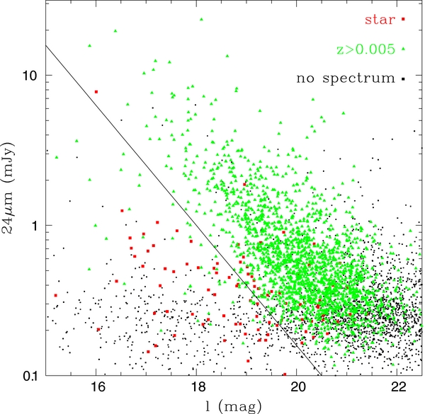
Figure 4. MIPS quasar selection. MIPS quasar targets are point sources with I(30) > 18–2.5log (F24/mJy). The green filled triangles show extragalactic sources, the filled red squares show stars, and the black squares are sources without spectroscopic confirmations. The black line indicates the color selection boundary. Targets appear below the line because of other targeting criteria.
Download figure:
Standard image High-resolution imageA galaxy target (galaxy = 1) was required to have pntsrc = 0, igood = 1 and one of rgood, bgood or zgood = 1. It then had to satisfy the (Kron-like) I-band magnitude criteria I ⩽ 20 mag, 10 aperture magnitude Iap1 ⩽ 24.0 and 60 aperture magnitude Iap6 ⩽ 21.0. A quasar target (qso = 1) had to have either igood = 1 or zgood = 1, which is more liberal than in 2005 because requirements on rgood or bgood could be problematic for very high redshift quasars. It then had to satisfy either I ⩽ 22.5 and a 10 aperture I-band magnitude Iap1 ⩽ 24 mag or that z' ⩽ 22.5 and a 10 z-band magnitude z'ap1 ⩽ 24.0 mag. We also included a separate category AGN/galaxy (agngalaxy = 1), which was an extended source that did not have to meet the criterion on the 60 aperture magnitude and included sources down to the faint limit used for the point sources I ⩽ 22.5 mag rather than the limit used for normal galaxies of I ⩽ 20 mag. The limit on the aperture magnitude is designed to filter out problems created by bright stars.
- 1.SDSS calibration stars (code06 = 1). These are SDSS stars with the colors of F stars that are used to flux calibrate the spectra.
- 2.Brown dwarf candidates (code06 = 2, qcode06 = 1). These are brown dwarf candidates (M. Ashby 2004, private communication). This sample is unchanged from 2005 other than through the modified definitions of galaxies and point sources.
- 3.Optical quasar candidates (code06 = 4, qcode06 = 2). These are BW/R/I/K-band color-selected quasar candidates (K. Brand & R. Green 2005, private communication). This sample is unchanged from 2005 other than through the modified definitions of galaxies and point sources.
- 4.WSRT radio sources (code06 = 8, qcode06 = 4). All sources (qso = 1, galaxy = 1, or agngalaxy = 1) within 30 of a 5σ detection in the WSRT 1.4 GHz survey of the field (de Vries et al. 2002). This differs from 2005 by including the faint, extended sources with agngalaxy = 1.
- 5.X-ray quasar candidates (code06 = 16, qcode06 = 8). All sources (qso = 1, galaxy = 1, or agngalaxy = 1) with 2 or more X-ray counts and a greater than 25% Bayesian probability of being identified with the optical source using the matching approach outlined in Brand et al. (2006). This differs from 2005 by including the faint, extended sources with agngalaxy = 1.
- 6.MIPS quasar candidates (code06 = 32, qcode06 = 16). This sample is unchanged from 2005 other than through the modified definitions of galaxies and point sources.
- 7.IRAC quasar candidates (code06 = 64, qcode06 = 32). This sample is the most heavily modified from 2005. The changes were implemented to better understand selection effects due to color and morphology. For point sources, it was clear from detailed analyses that the old color criterion led to reduced completeness whenever a bright emission line was in the 3.6 μm band, in particular at z ∼ 4.5 with the Hα line (see Assef et al. 2010). It was also clear that the differing magnitude limits for point and extended sources were a significant problem at low redshifts. The new selection criterion were sufficiently complex that we introduced a separate code (iracq06) to label the various criteria. We also switched to using colors measured with positions set by the 3.6 μm band ([x][3.6] magnitudes rather than [x]x magnitudes).
- 8.MIPS 24 μm galaxy sample (code06 = 128, gcode06 = 1). This sample is unchanged from 2005 other than through the modified definitions of galaxies and point sources.
- 9.IRAC channel 4 (8.0 μm) galaxy sample (code06 = 256, gcode06 = 2). This sample is unchanged from 2005 other than through the modified definitions of galaxies and point sources.
- 10.IRAC channel 3 (5.8 μm) galaxy sample (code06 = 512, gcode06 = 4). This sample is unchanged from 2005 other than through the modified definitions of galaxies and point sources.
- 11.IRAC channel 2 (4.5 μm) galaxy sample (code06 = 1024, gcode06 = 8). This sample is unchanged from 2005 other than through the modified definitions of galaxies and point sources.
- 12.IRAC channel 1 (3.6 μm) galaxy sample (code06 = 2048, gcode06 = 16). This sample is unchanged from 2005 other than through the modified definitions of galaxies and point sources.
- 13.GALEX FUV-band galaxy sample (code06 = 4096, gcode06 = 32). This sample was rebuilt from the public GALEX catalogs available for the field in 2007, within 0.45 deg of the GALEX field center and with at least 2000 sec of NUV integration time. The GALEX data still covered only a modest fraction of the standard fields.
- 14.GALEX NUV-band galaxy sample (code06 = 8192, gcode06 = 64). This sample was rebuilt from the public GALEX catalogs available for the field in 2007, within 0.45 deg of the GALEX field center and with at least 2000 sec of NUV integration time.
- 15.K-band galaxy sample (code06 = 16384, gcode06 = 128). This sample is unchanged from 2005 other than through the modified definitions of galaxies and point sources.
- 16.J-band galaxy sample (code06 = 32768, gcode06 = 256). This sample is unchanged from 2005 other than through the modified definitions of galaxies and point sources.
- 17.BW-band galaxy sample (code06 = 65536, gcode06 = 512). This sample is unchanged from 2005 other than through the modified definitions of galaxies and point sources.
- 18.R-band galaxy sample (code06 = 131072, gcode06 = 1024). This sample is unchanged from 2005 other than through the modified definitions of galaxies and point sources.
- 19.Other I-band galaxies (code06 = 262144, gcode06 = 2048). This sample is unchanged from 2005 other than through the modified definitions of galaxies and point sources.
- 20.Main I-band galaxy sample (code06 = 524288, gcode06 = 4096). This sample is unchanged from 2005 other than through the modified definitions of galaxies and point sources.
3. OBSERVATIONS
The observations were made with Hectospec (Fabricant et al. 1998, 2005; Roll et al. 1998), a 300 fiber, 1 degree field of view, robotic spectrograph for the 6.5 m MMT telescope at Mt. Hopkins. The wavelength range is 3700 Å–9200 Å with a pixel scale of 1.2 Å and a spectral resolution of 6 Å (i.e., roughly R ∼ 1000). The throughput at the wavelength extremes is low, and an infrared LED in the fiber robots contaminates some spectra redward of 8500 Å, with an amplitude that depends on the proximity of the fiber to the source. The fibers have a diameter of only 15. We generically aimed for 30 sky fibers, sometimes obtaining more if there was a shortage of targets, and 3–5 SDSS F-star candidates for flux calibration.
In 2004 we tried to put 20 of the sky fibers on blank sky positions selected from the SDSS imaging data for the field and the rest at random positions, but eventually switched to simply using random positions as it became clear that contamination of the sky fibers by sources was not a significant problem. In the first runs in 2004 the atmospheric dispersion corrector was not working properly (see Table 2), which means that some of the spectra could not be properly flux calibrated and there are significant spectral distortions unless the data were obtained very close to the zenith. The guide cameras are primarily red sensitive, so the fibers generally were properly positioned for the red light while the bluer wavelengths were systematically shifted, sometimes leading to quite dramatic losses for blue emission from point sources.
Observations are described by a three digit pass number ABB where, in general, A indicates the sequential pass over the fields and BB indicates the field. So, pass 203 would be the second pointing at sub-field 3. The individual pointings were not exactly centered on the fields, but were shifted to help maximize the overall completeness. Weather problems, leading to repeated observations, the longevity of the project, and the introduction of co-added spectra from multiple observations eventually led to a partial break down in the naming scheme. Table 2 summarizes all the observations.
In 2004 we carried out three passes with integration times of 24, 45, and 75 minutes divided into 2, 3, and 4 exposures respectively. The targets were divided into surface brightness classes with the high, medium, and low surface brightness targets assigned to the short, medium, and long integration times. Targets with failed redshifts in the first passes were recycled for observations in the later, deeper passes. The systematic recycling of failures during this and later seasons means that fiber collisions are largely irrelevant to the completeness of any of the AGES samples.
The 2005 observations used pass numbers of 4 through 7, indicating the month of the observation (March, April, May, and June/July), and field numbers of 1⋅⋅⋅26, where 1⋅⋅⋅15 correspond to the standard sub-fields, 16⋅⋅⋅21 to observations in the boundary regions, and 22⋅⋅⋅26 to repeat observations in the 15 standard sub-fields. The exposure times were generally 90 minutes. Experiments using 54 minute exposure times had poor redshift yields. The observing conditions were not homogeneous, with significant variations in the signal-to-noise ratios (S/Ns) beyond the effects of the changing exposure times.
In 2006 we had less time and terrible weather. All the observations were designated as pass 8, where in the first run we observed fields 1–5 (801, 802, 803, 804, 805). The poor yields led us to repeat these observations in the second run (these we labeled by the field number plus twenty, so 821, 822, 823, 824, 825, and 834 for observations of fields 1, 2, 3, 4, 5, and 14, and there was one additional observation of field 1 labeled 841). We also produced co-added spectra of all multiply observed targets that were assigned codes of 861, 862, and 863. In 2007 we tried to focus on fields with lower completeness levels. These were numbered in the 900's, again adding 20 to the pass number when a field was re-observed.
Quasars with redshift z > 2.4 were repeatedly reobserved until the co-added spectrum yielded an S/N above 10/pixel. The objective was to build a clean sample for potentially studying correlations in Lyα forest absorption. SDSS redshifts are marked as pass/aperture 0/0 entries.
4. DATA REDUCTION
The data were reduced by two separate pipelines, the standard Hectospec pipeline at the Center for Astrophysics (CfA) and a modified SDSS pipeline, HSRED.
In the CfA pipeline the separate exposures were de-biased and flat fielded using exposures of the MMT ceiling illuminated by a continuum lamp (the latter exposures had the lamp spectral shape removed by the IRAF program "apflatten"). The object exposures were then compared before extraction to allow identification and elimination of cosmic rays through interpolation. Spectra were then extracted from individual exposures using the variance weighting method, wavelength calibrated and combined. Each fiber has a distinct wavelength dependence in throughput, which can be estimated using flat field exposures or the twilight sky. The object spectra were next corrected for this dependence, followed by a correction to put all the spectra on the same exposure level. The latter correction was estimated by the strength of several night sky emission lines. Sky subtraction was performed, using object-free spectra as near as possible to each target. Small corrections to the wavelength zero point based on the wavelengths of night sky emission lines were then applied. Finally, redshifts were estimated by cross correlation with emission/absorption line galaxy and AGN template spectra. The CfA pipeline spectra are then the average of the extracted spectra in counts.
For HSRED, the observations of the flat-field screen taken in the afternoon were again used to correct for the high-frequency flat-field variations and fringing in the CCD. We removed low-frequency fiber-to-fiber transmission differences using observations of the twilight sky. Wavelength solutions were obtained each night using observations of HeNeAr calibration lamps, and the locations of strong emission lines in the spectrum of the night sky were used to correct for any drift in the wavelength solution between observations of the calibration frames and the data frames. Each Hectospec configuration has approximately 30 fibers dedicated to measuring the sky spectrum. These sky observations were used to create a median sky spectrum for each exposure, which was interpolated and subtracted from each object spectrum. Simultaneous observations of F-type stars in each configuration were cross-correlated against a grid of Kurucz models to derive a sensitivity function for each observation, thus linking the observed counts to absolute flux units. Where flux calibration is successful, the HSRED spectra are Fλ in units of 10−17 erg cm−2 s−1 Å−1.
Redshifts were determined using programs available in the IDLSPEC2D package of IDL routines developed for the SDSS. To determine the redshift of each object in the survey, we compared the observed spectra with empirical stellar, galaxy, and quasar template models included in the IDLSPEC2D package and allowed the strength of the emission lines present in the object to be fit simultaneously with the redshift of the galaxy. The final redshift and object classification were determined by selecting the template and redshift combination that minimized the χ2 between model and data.
All spectra were visually inspected, usually by two individuals (C.S.K. and D.J.E.), with a particular focus on low-S/N spectra and spectra where the two pipelines produced discrepant redshifts. These were then either flagged as wrong, adjusted to the correct value, or analyzed manually.
5. A SUMMARY OF THE SURVEY
The general properties of the survey are summarized in Tables 1, 3, and 4 and illustrated in Figures 2, 5, and 6. Table 1 and Figure 2 illustrate the spatial completeness of the survey using the main I-band galaxy sample. In the standard sub-fields, spectra were attempted for 96.6% of this sample, and redshifts were measured for 93.6%. The completeness is worst for fields 13, 14, and 15, both in terms of the fraction of attempts (86%–91%) and the overall completeness (83%–89%). Two factors led to the lower completeness. First, all three of the fields have more targets (786, 748, and 855 respectively) than the mean (734 per field), although we achieved much higher completenesses for other dense fields such as field 4. Second, we emphasized completing the lower field numbers in the face of poor weather and limited time to finish our observations. Every field was observed many times (see Table 2), so fiber collisions play a very small role in the incompleteness.

Figure 5. Completeness as a function of the random sparse sampling rcode (see Section 2.2) for all I < 20 mag galaxies, where each rcode bin contains an average of 5% of the targets (1959 for the I < 20 mag galaxies). The dashed line indicates the fraction with spectra and the solid line indicates the fraction with measured redshifts. The horizontal line shows the mean completeness and the vertical lines mark the 20% and 30% sparse sampling goals for the main I-band sample and the other galaxy samples, respectively.
Download figure:
Standard image High-resolution image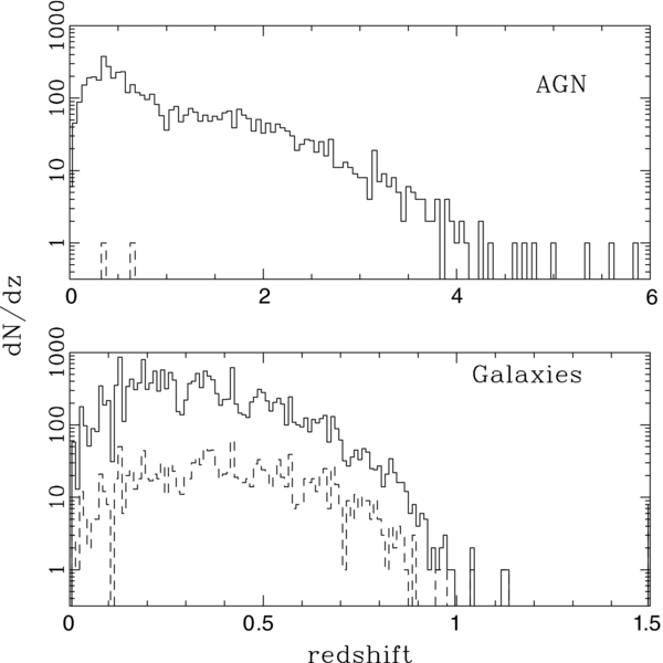
Figure 6. Redshift distributions of AGNs (top) and galaxies (bottom). In the top panel the solid (dashed) histograms are for point (extended) sources with an AGN targeting code (qcode06 > 3). In the lower panel, the solid histograms show all objects targeted as galaxies (gcode06 > 0), and the dashed histograms show the objects targeted as galaxies that also had an AGN targeting code (qcode06 > 3).
Download figure:
Standard image High-resolution imageTable 3 summarizes the 2006/2007 samples, excluding the flux calibration stars, and brown dwarf and optical quasar test samples. The well-defined galaxy samples are very complete, with the main I-band sample having the lowest completeness (94%), followed by the MIPS sample (95%). The remainder have completenesses above 98%. The GALEX samples are spatially inhomogeneous and of limited use. In total, we obtained redshifts for roughly 61% of the galaxies with I < 20 mag.
Figure 5 shows the completeness as a function of the random sample code. Because we emphasized observing lower rcodes, it is relatively easy to rapidly increase the size of the sample with high completeness. The main I-band galaxy sample used 20% sparse sampling (rcode ⩽ 3) for its fainter magnitudes, 18.5 ⩽ I ⩽ 20, while the IR samples used 30% sparse sampling (rcode ⩽ 5). The higher rcodes were assigned priorities that dropped with every increase in the rcode by two, leading to the steady drop in the completeness. With this design, little effort is needed to produce significantly larger complete samples. About 500 redshifts are needed to complete the main galaxy sample. Another 1600 would complete the sample to a sparse sampling fraction between 18.5 < I < 20 of 40%.
In total we selected almost 8977 objects as AGN candidates, took spectra of 7102, and obtained redshifts for 5217, of which 4764 were not Galactic stars. Table 4 summarizes the completeness of the various categories of AGNs, breaking the statistics into the various sub-samples (point source, bright extended sources, faint extended sources) and giving statistics for all the AGN selection methods (all objects with an AGN selection code) as compared to the total galaxy sample (all objects with code06 ⩾ 128). In total, we identified 1718 AGNs with z > 1 in the field, a surface density of more than 200 deg−2. Three quasars with redshifts above 5 were identified (Cool et al. 2006). A redshift 6.12 quasar was targeted as an IRAC AGN but not observed before it was discovered by McGreer et al. (2006) and Stern et al. (2007). The completenesses for the point source and bright extended AGNs are generally good, while that for the fainter extended AGN candidates is very poor. Figure 6 shows the redshift distributions of the galaxy and AGN populations.
The different AGN selection methods emphasize different galaxy types and redshift ranges, as discussed in more detail by Hickox et al. (2007), Gorjian et al. (2008), Assef et al. (2010), and Assef et al. (2011). Figure 7 illustrates some of these issues using a Venn diagram adapted from Assef et al. (2010) showing the overlap between the WSRT, X-ray, IRAC, and MIPS quasar selection methods for several different redshift ranges. The primary difference between the X-ray (and radio) sample versus the IRAC and MIPS samples is that X-ray selection is essentially independent of host properties while the IRAC and MIPS samples are not. Thus, lower redshift AGNs are more likely to be X-ray selected because the generally larger contribution of the host galaxy at lower redshifts changes the mid-IR colors or makes the optical counterpart to the MIPS source non-point-like. On the other hand, the mid-IR selection methods may well be better for finding moderately obscured quasars where the soft X-ray photons to which Chandra is most sensitive are absorbed. Many of these problems could be solved using the Assef et al. (2010) template models to fit the complete photometry for each source and target those with any evidence of an AGN contribution.

Figure 7. Venn diagrams illustrating the degree of overlap between the primary AGN selection methods (IRAC mid-IR, MIPS 24 μm, X-ray, and radio). The panels show the divisions for all (top panel), lower redshift (z < 1, middle panel), and higher redshift (z > 1, lower panel) AGNs. For any one of the selection methods, there are eight possible overlaps ranging from no other method to all three other methods.
Download figure:
Standard image High-resolution image6. DATA RELEASE
The AGES data release consists of a series of row-matched tables. They do not contain all entries from the matched photometric catalogs, as these contain far more information than is needed to interpret the AGES data. We have also included only the final photometry used in later observing seasons. We do not report the photometry associated with the intermediate states because the completeness of the final samples is so high. We do report the selection codes used in the earlier observing seasons so that the history of the targeting can be traced if necessary and to explain the origin of the small numbers sources with redshifts that were not explicitly targeted in the final seasons.
Table 5 summarizes the selection codes for each source. This includes the 2004, 2005 and 2006/2007 targeting codes, the field IDs, the random sparse sampling code, the bright star flag, the IRAC AGN sub-sample code, and the flags for whether the source was considered a standard galaxy, a quasar, a point source, or a fainter galaxy that was an AGN candidate.
Table 5. Summary of Selection Codes and Flags
| R.A. | Decl. | Code06 | Code05 | Code04 | rcode | field | bstar | qirac | gal | qso | pntsrc | agngal |
|---|---|---|---|---|---|---|---|---|---|---|---|---|
| 217.375476 | 32.806272 | 720896 | 720896 | 1536 | 0 | 8 | 0 | 0 | 1 | 0 | 0 | 1 |
| 217.893029 | 32.806415 | 724480 | 724480 | 2076 | 2 | 0 | 0 | 0 | 1 | 0 | 0 | 1 |
| 217.297011 | 32.806733 | 112 | 112 | 288 | 6 | 0 | 0 | 1 | 0 | 1 | 1 | 0 |
| 217.304623 | 32.806823 | 262144 | 262144 | 1024 | 6 | 0 | 0 | 0 | 1 | 0 | 0 | 1 |
| 216.311008 | 32.808259 | 589824 | 589824 | 1088 | 11 | 4 | 0 | 0 | 1 | 0 | 0 | 1 |
| 216.333753 | 32.806956 | 524288 | 524288 | −1 | 16 | 4 | 0 | 0 | 1 | 0 | 0 | 1 |
| 216.393848 | 32.806964 | 724864 | 724864 | 2174 | 12 | 4 | 0 | 0 | 1 | 0 | 0 | 1 |
| 216.644254 | 32.806900 | 720896 | 720896 | 2112 | 10 | 4 | 0 | 0 | 1 | 0 | 0 | 1 |
| 217.088601 | 32.807106 | 262656 | 262784 | −1 | 18 | 0 | 0 | 0 | 1 | 0 | 0 | 1 |
| 217.086404 | 32.807395 | 721152 | 721152 | 2112 | 11 | 0 | 0 | 0 | 1 | 0 | 0 | 1 |
| 217.479422 | 32.807504 | 524288 | 524288 | −1 | 0 | 8 | 0 | 0 | 1 | 0 | 0 | 1 |
| 216.548230 | 32.807663 | 655360 | 655360 | 1536 | 3 | 4 | 0 | 0 | 1 | 0 | 0 | 1 |
| 217.228471 | 32.807886 | 262144 | 262144 | −1 | 13 | 0 | 0 | 0 | 1 | 0 | 0 | 1 |
| 216.206669 | 32.808026 | 262144 | 262144 | −1 | 10 | 4 | 0 | 0 | 1 | 0 | 0 | 1 |
| 216.199841 | 32.808199 | 16 | −1 | −1 | 5 | 4 | 0 | 0 | 0 | 1 | 0 | 1 |
| 216.845202 | 32.808131 | 262144 | 262144 | 1024 | 12 | 4 | 0 | 0 | 1 | 0 | 0 | 1 |
| 217.467032 | 32.808139 | 262272 | 262272 | 1024 | 12 | 8 | 0 | 0 | 1 | 0 | 0 | 1 |
| 216.328172 | 32.808479 | −658432 | 0 | −1 | 14 | 4 | 0 | 0 | 1 | 0 | 0 | 1 |
| 216.584225 | 32.808667 | 458752 | 458752 | 2112 | 10 | 4 | 0 | 0 | 1 | 0 | 0 | 1 |
| 217.618515 | 32.808876 | 524288 | 524288 | −1 | 3 | 0 | 0 | 0 | 1 | 0 | 0 | 1 |
Notes. Code06, Code05, Code04 are the binary sample selection codes for the 2006/2007 (see Section 2.7), 2005 (see Section 2.6), and 2004 (see Section 2.5) survey periods, rcode is the random sample code, with each index representing a randomly selected 5% of the sources, field is the sub-field number, where 0 indicates that it is outside the standard fields. "qirac" gives the IRAC AGN selection sub-code for the 2006/2007 season. In 340 cases likely to be semi-saturated stars, we report −Code06. The codes gal, qso, pntsrc, and agngal indicate whether the source was counted as a galaxy target, an AGN target, a point source, or a faint (I > 20 mag) extended AGN candidate. See Section 2 for a detailed definitions and discussions of the entries. The R.A. and Decl. in this and later tables are the NDWFS DR3 I-band coordinates.
Only a portion of this table is shown here to demonstrate its form and content. A machine-readable version of the full table is available.
Download table as: DataTypeset image
Table 6 presents the photometry for the sources from XBoötes (Murray et al. 2005; Kenter et al. 2005; Brand et al. 2006), GALEX (Martin et al. 2005), NDWFS DR3 (Jannuzi & Dey 1999), zBoötes (Cool 2007), FLAMEX (Elston et al. 2006), the IRAC Shallow Survey (Eisenhardt et al. 2004), and Soifer & Spitzer/NOAO Team (2004). The X-ray photometry is in counts for sources with a 25% or greater Bayesian match probability in Brand et al. (2006). The NDWFS, FLAMEX and IRAC Shallow Survey are the (Kron-like/mag auto) Vega magnitudes, GALEX, and zBoötes are in AB magnitudes, and the 24 μm flux is in mJy. Objects with unusual photometric properties should be inspected closely before use. Table 7 summarizes the spectroscopy, listing the number of spectra taken, the estimated redshifts, the (continuum) S/N of the spectra, and the pass/aperture identification code for each spectrum. Figure 8 shows three examples of spectra of galaxies illustrating the quality for (continuum) signal-noise-ratios representative of the worst 5%, median, and best 5% of the sample. Figure 9 does the same for three examples of quasar spectra. The signal-to-noise estimate in Table 7 is an indicator of redshift reliability, as well as any agreements/disagreements between repeated low signal-to-noise spectra.
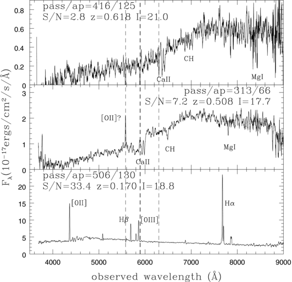
Figure 8. Three examples of the spectra of galaxies. The top, middle, and lower panels show spectra with continuum signal-to-noise ratios typical of the worst 5%, median, and best 5% of the spectra yielding redshifts, respectively. Several features are labeled, and the vertical lines mark the strong sky lines. The spectra are smoothed by an 11 pixel box car, which roughly halves the intrinsic spectral resolution.
Download figure:
Standard image High-resolution image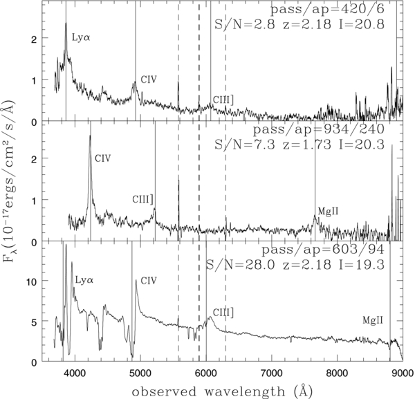
Figure 9. Three examples of the spectra of quasars. The top, middle, and lower panels show spectra with continuum signal-to-noise ratios typical of the worst 5%, median, and best 5% of the spectra yielding redshifts. Several features are labeled and marked by the solid vertical lines while the dashed lines mark the strongest sky lines. The spectra are smoothed by an 11 pixel box car. The strong (BAL) absorption features in the bottom spectrum have biased the pipeline redshift estimate.
Download figure:
Standard image High-resolution image
Table 6. Magnitudes And Fluxes
| X | FUV | NUV | BW | R | I | z' | J | K1 | K2 | [3.6] | [4.5] | [5.8] | [8.0] | 24 |
|---|---|---|---|---|---|---|---|---|---|---|---|---|---|---|
| −10 | −10.00 | −10.00 | 20.71 | 19.29 | 18.77 | 19.13 | −10.00 | −10.00 | −10.00 | 16.63 | 16.45 | −10.00 | 14.02 | −10.000 |
| −10 | −10.00 | 24.52 | 20.78 | 18.15 | 17.43 | 17.63 | −10.00 | −10.00 | −10.00 | 14.53 | 14.46 | 14.40 | 14.27 | −10.000 |
| 3 | −10.00 | −10.00 | 18.52 | 18.20 | 17.87 | 18.38 | −10.00 | −10.00 | −10.00 | 14.66 | 13.72 | 12.85 | 11.81 | 3.474 |
| −10 | −10.00 | −10.00 | 20.89 | 19.77 | 19.31 | 19.71 | −10.00 | −10.00 | −10.00 | 17.44 | 17.51 | −10.00 | −10.00 | −10.000 |
| −10 | −10.00 | −10.00 | 20.43 | 19.71 | 17.27 | 19.77 | −10.00 | −10.00 | −10.00 | −10.00 | 16.81 | −10.00 | 15.47 | −10.000 |
| −10 | −10.00 | −10.00 | −10.00 | 20.94 | 18.22 | 21.51 | −10.00 | −10.00 | −10.00 | −10.00 | −10.00 | −10.00 | −10.00 | −10.000 |
| −10 | −10.00 | −10.00 | 18.98 | 17.32 | 16.64 | 16.93 | −10.00 | −10.00 | −10.00 | 14.00 | 13.94 | 13.29 | 10.82 | 2.775 |
| −10 | −10.00 | −10.00 | 20.45 | 18.64 | 17.89 | −10.00 | −10.00 | −10.00 | −10.00 | 16.53 | 16.52 | −10.00 | 14.93 | −10.000 |
| −10 | −10.00 | −10.00 | 22.25 | 20.01 | 19.15 | 19.29 | −10.00 | −10.00 | −10.00 | 15.58 | 15.45 | 14.27 | 14.13 | 0.467 |
| −10 | −10.00 | −10.00 | 20.29 | 18.59 | 17.95 | 18.14 | −10.00 | −10.00 | −10.00 | 15.55 | 15.25 | −10.00 | 12.94 | −10.000 |
| −10 | −10.00 | 23.07 | 22.25 | 20.52 | 19.88 | 20.32 | −10.00 | −10.00 | −10.00 | 17.18 | 16.51 | −10.00 | 15.00 | −10.000 |
| −10 | −10.00 | −10.00 | 22.08 | 19.92 | 19.21 | 19.38 | −10.00 | −10.00 | −10.00 | 16.03 | 15.72 | 15.79 | 15.23 | −10.000 |
| −10 | −10.00 | −10.00 | 23.11 | 20.25 | 19.34 | 19.54 | −10.00 | −10.00 | −10.00 | 16.14 | 16.05 | 16.14 | −10.00 | −10.000 |
| −10 | −10.00 | −10.00 | 23.73 | 20.52 | 19.40 | 19.83 | −10.00 | −10.00 | −10.00 | −10.00 | 15.99 | −10.00 | 15.74 | −10.000 |
| 4 | −10.00 | −10.00 | 22.31 | 22.04 | 21.53 | 21.95 | −10.00 | −10.00 | −10.00 | −10.00 | 16.95 | −10.00 | 15.44 | −10.000 |
| −10 | −10.00 | −10.00 | 21.50 | 19.65 | 18.98 | 19.35 | −10.00 | −10.00 | −10.00 | 16.39 | 16.21 | 16.20 | 13.98 | 0.342 |
| −10 | −10.00 | 23.29 | 21.77 | 19.82 | 19.10 | 19.39 | −10.00 | −10.00 | −10.00 | 15.87 | 15.46 | 15.15 | 13.67 | 0.693 |
| −10 | −10.00 | −10.00 | 23.78 | 14.81 | 13.76 | 20.58 | −10.00 | −10.00 | −10.00 | 13.68 | 13.39 | −10.00 | −10.00 | −10.000 |
| −10 | −10.00 | −10.00 | 20.36 | 19.15 | 18.67 | 19.07 | −10.00 | −10.00 | −10.00 | 16.81 | 16.56 | −10.00 | 14.24 | −10.000 |
| −10 | −10.00 | −10.00 | 23.09 | 20.57 | 19.79 | 19.84 | −10.00 | −10.00 | −10.00 | 16.77 | 16.57 | −10.00 | 14.78 | −10.000 |
Notes. All entries except the X-ray column (X, counts) and 24 μm column (24, mJy) are in Vega magnitudes. An entry of −10 means no data or below the magnitude limit of the survey. X is from XBoötes (Murray et al. 2005; Kenter et al. 2005; Brand et al. 2006), FUV and NUV are from GALEX (Martin et al. 2005), BW, R, I, and K2 are from the NDWFS DR3 (Jannuzi & Dey 1999), z' is from zBoötes (Cool 2007), J and K1 are from FLAMEX (Elston et al. 2006), [3.6]−[8.0] are from the IRAC Shallow Survey (Eisenhardt et al. 2004), and the MIPS 24 μm fluxes are from Soifer & Spitzer/NOAO Team (2004).
Only a portion of this table is shown here to demonstrate its form and content. A machine-readable version of the full table is available.
Download table as: DataTypeset image
Table 7. Redshifts
| R.A. | Decl. | N | Spectrum 1 | Spectrum 2 | Spectrum 3 | |||||||||
|---|---|---|---|---|---|---|---|---|---|---|---|---|---|---|
| z | S/N | pass | ap | z | S/N | pass | ap | z | S/N | pass | ap | |||
| 217.375476 | 32.806272 | 1 | 0.219 | 9.009 | 308 | 230 | ||||||||
| 217.893029 | 32.806415 | 0 | ||||||||||||
| 217.297011 | 32.806733 | 1 | 1.257 | 34.483 | 108 | 100 | ||||||||
| 217.304623 | 32.806823 | 1 | 0.136 | 21.703 | 948 | 212 | ||||||||
| 216.311008 | 32.808259 | 2 | 0.352 | 2.745 | 604 | 100 | −1.352 | 2.806 | 423 | 225 | ||||
| 216.333753 | 32.806956 | 0 | ||||||||||||
| 216.393848 | 32.806964 | 2 | 0.094 | 20.408 | 304 | 232 | 0.095 | 0.000 | 0 | 1 | ||||
| 216.644254 | 32.806900 | 1 | 0.131 | 3.534 | 204 | 90 | ||||||||
| 217.088601 | 32.807106 | 0 | ||||||||||||
| 217.086404 | 32.807395 | 1 | 0.132 | 15.873 | 304 | 177 | ||||||||
| 217.479422 | 32.807504 | 1 | 0.346 | 5.782 | 417 | 56 | ||||||||
| 216.548230 | 32.807663 | 1 | 0.248 | 9.615 | 304 | 213 | ||||||||
| 217.228471 | 32.807886 | 0 | ||||||||||||
| 216.206669 | 32.808026 | 1 | 0.534 | 2.297 | 604 | 102 | ||||||||
| 216.199841 | 32.808199 | 3 | 1.954 | 5.503 | 862 | 272 | 1.954 | 4.998 | 824 | 250 | 1.954 | 1.768 | 804 | 211 |
| 216.845202 | 32.808131 | 2 | 0.217 | 19.907 | 862 | 231 | 0.217 | 16.113 | 804 | 165 | ||||
| 217.467032 | 32.808139 | 1 | 0.346 | 9.655 | 608 | 181 | ||||||||
| 216.328172 | 32.808479 | 1 | −4.218 | 3.240 | 404 | 199 | ||||||||
| 216.584225 | 32.808667 | 1 | 0.170 | 9.615 | 304 | 220 | ||||||||
| 217.618515 | 32.808876 | 0 | ||||||||||||
Notes. N indicates the number of spectra taken. The redshift z, signal-to-noise ratio S/N, pass, and aperture codes (see Section 4) are then given for up to the first three spectra in order of decreasing S/N. Pipeline redshifts that did not pass visual inspection are reported as −1 − z, where z was the pipeline redshift estimate.
Only a portion of this table is shown here to demonstrate its form and content. A machine-readable version of the full table is available.
Download table as: DataTypeset image
Table 8 provides photometric redshift estimates and template decompositions for each object's photometry following Assef et al. (2010). The SED is fit as a combination of an early-type, late-type, star forming, and (obscured) AGNs for the full range of available UV/optical/near-IR/far-IR photometry, and we report the luminosities associated with each component and the extinction applied to the AGN template. Where a spectroscopic redshift is available, the template decomposition is carried out at the spectroscopic redshift. The accuracy of the photometric redshifts is σz = 0.04/(1 + z) for galaxies, and Assef et al. (2010) should be consulted for a detailed discussion of the results for strong AGNs.
Table 8. Photometric Redshifts
| R.A. | Decl. | Nband | zphot | χ2 | E | Sbc | Im | AGN | E(B − V) |
|---|---|---|---|---|---|---|---|---|---|
| (Luminosity L/1010 L☉) | (mag) | ||||||||
| 217.375476 | 32.806272 | 9 | 0.160 | 1.443 | 0.238 | 0.168 | 0.351 | 0.052 | 0.184 |
| 217.893029 | 32.806415 | 9 | 0.260 | 2.347 | 6.906 | 0.000 | 0.000 | 0.085 | 0.359 |
| 217.297011 | 32.806733 | 10 | 0.120 | 15.820 | 0.000 | 0.000 | 1.090 | 0.039 | 0.048 |
| 217.304623 | 32.806823 | 9 | 0.220 | 9.626 | 0.242 | 0.000 | 0.715 | 0.072 | 0.000 |
| 216.311008 | 32.808259 | 9 | 0.580 | 49.400 | 0.000 | 1.348 | 1.464 | 0.190 | 0.184 |
| 216.333753 | 32.806956 | 9 | 0.600 | 22.913 | 1.230 | 0.000 | 0.541 | 0.197 | 0.147 |
| 216.393848 | 32.806964 | 9 | 0.140 | 13.895 | 0.000 | 3.627 | 0.000 | 0.046 | 0.450 |
| 216.644254 | 32.806900 | 7 | 0.220 | 0.990 | 0.535 | 0.055 | 0.336 | 0.072 | 0.000 |
| 217.088601 | 32.807106 | 8 | 0.460 | 0.887 | 4.222 | 2.537 | 0.000 | 0.151 | 0.094 |
| 217.086404 | 32.807395 | 8 | 0.140 | 1.463 | 0.663 | 0.337 | 0.220 | 0.046 | 0.000 |
| 217.479422 | 32.807504 | 9 | 0.280 | 2.062 | 0.024 | 1.042 | 0.270 | 0.092 | 0.000 |
| 216.548230 | 32.807663 | 8 | 0.340 | 0.408 | 2.185 | 0.435 | 0.327 | 0.112 | 0.000 |
| 217.228471 | 32.807886 | 8 | 0.440 | 0.507 | 4.339 | 0.000 | 0.001 | 0.144 | 0.094 |
| 216.206669 | 32.808026 | 8 | 0.500 | 1.835 | 4.987 | 0.000 | 0.000 | 0.164 | 0.230 |
| 216.199841 | 32.808199 | 8 | 0.680 | 2.961 | 0.000 | 1.143 | 0.000 | 0.223 | 0.048 |
| 216.845202 | 32.808131 | 9 | 0.220 | 1.132 | 0.600 | 0.702 | 0.166 | 0.072 | 0.000 |
| 217.467032 | 32.808139 | 9 | 0.280 | 0.386 | 0.034 | 2.940 | 0.000 | 0.092 | 0.147 |
| 216.328172 | 32.808479 | 7 | 1.000 | 86.301 | 2.305 | 12.494 | 0.000 | 0.328 | 0.000 |
| 216.584225 | 32.808667 | 10 | 0.100 | 4.412 | 0.105 | 0.039 | 0.167 | 0.033 | 0.184 |
| 217.618515 | 32.808876 | 9 | 0.360 | 2.089 | 1.306 | 0.870 | 0.070 | 0.118 | 0.000 |
Notes. Photometric redshift and SED decompositions following Assef et al. (2010). Nband is the number of bands used to derive the photometric redshift zphot and χ2 is the goodness of fit at the photometric redshift. The E, Sbc, Im, and AGN columns give the contributions of these templates to the SED in units of 1010 L☉. By definition the contributions are always ⩾0, and they are calculated for the spectroscopic redshift if it is known. The AGN luminosity is only calculated redward of the Lyman limit. E(B − V) is the extinction applied to the AGN template.
Only a portion of this table is shown here to demonstrate its form and content. A machine-readable version of the full table is available.
Download table as: DataTypeset image
As discussed in Section 4, the NDWFS SExtractor Kron-like magnitudes IAUTO tend to overestimate source fluxes near bright stars. In Cool et al. (2012), we developed a method to produce a corrected estimate, which we summarize here. Let IR = RAUTO + (I(60) − R(60))) be the I-band magnitude predicted from the R-band Kron-like magnitude RAUTO and the 60 aperture color. The surrogate I-band total magnitude
where f = exp (− (IAUTO − IR)2/0.22) is a weight factor. On average 〈Itot − IAUTO〉 = 0.005 mag with an rms scatter of 0.02 mag, but 10% (5%) of galaxies have shifts of 0.1 (0.5) mag.
Completeness corrections for the galaxy samples are relatively straightforward. Cool et al. (2012) discusses several tests of the completeness of the input catalogs, coming to the conclusion that the catalog completeness is of order 96%–97%, largely due to the loss of faint objects superposed on brighter galaxies or stars. There are very few spurious objects. Only 1% of the main-sample galaxies lack counterparts in SDSS imaging, although some saturated stars were misidentified as galaxy targets. These are easily identified because the resulting spectra and redshifts are stellar. The remaining issues are the sparse sampling fractions, fiber allocation completeness, and redshift failure rates. Following Cool et al. (2012), Table 9 provides the completeness corrections for the galaxy samples as well as the maximum redshift at which the galaxy would have entered the AGES sample and the corresponding volume Vmax for the galaxy to have been included in the survey with I < 20 mag assuming no evolution.
Table 9. Completeness and K-corrections for the Galaxy Samples
| R.A. | Decl. | Completeness Corrections | zmax | Vmax | ||
|---|---|---|---|---|---|---|
| Spec | Sparse | Fiber | (106 h−3 Mpc3) | |||
| 217.375476 | 32.806272 | 1.029 | 5.000 | 1.004 | 0.391 | 0.928 |
| 217.893029 | 32.806415 | |||||
| 217.297011 | 32.806733 | |||||
| 217.304623 | 32.806823 | |||||
| 216.311008 | 32.808259 | 1.054 | 1.000 | 1.004 | 2.346 | 47.569 |
| 216.333753 | 32.806956 | |||||
| 216.393848 | 32.806964 | 1.000 | 1.000 | 1.002 | 0.423 | 1.148 |
| 216.644254 | 32.806900 | 1.000 | 1.000 | 1.004 | 0.335 | 0.611 |
| 217.088601 | 32.807106 | |||||
| 217.086404 | 32.807395 | 1.000 | 1.000 | 1.000 | 0.335 | 0.609 |
| 217.479422 | 32.807504 | 1.040 | 5.000 | 1.307 | 0.364 | 0.768 |
| 216.548230 | 32.807663 | 1.003 | 5.000 | 1.004 | 0.355 | 0.719 |
| 217.228471 | 32.807886 | |||||
| 216.206669 | 32.808026 | 0.687 | 3.975 | |||
| 216.199841 | 32.808199 | |||||
| 216.845202 | 32.808131 | |||||
| 217.467032 | 32.808139 | 1.006 | 1.000 | 1.307 | 0.521 | 1.987 |
| 216.328172 | 32.808479 | |||||
| 216.584225 | 32.808667 | 1.006 | 1.000 | 1.002 | 0.322 | 0.547 |
| 217.618515 | 32.808876 | |||||
Notes. Factors needed to properly weight the galaxy samples following Cool et al. (2012). There are three completeness corrections factors. "Spec" corrects for the failure to determine a redshift when a spectrum was obtained, "Sparse" corrects for the target sparse sampling weighting, and "Fiber" corrects for how the local target density affects the assignment of fibers. The sparse sampling weights are non-zero only for galaxies in the main statistical samples, meaning sources in one of the 15 standard fields with at least one galaxy selection code other than "Other I band" (262144). The sparse sampling weight is then simply the inverse of the largest sampling rate used for any of the valid selection codes (100%, 30%, or 20%). The maximum redshift at which the source would have included the target is zmax and this corresponds to a volume of Vmax in units of 106 h−3 Mpc3 for an Ω = 0.3, Λ = 0.7 cosmological model and the survey area of 7.60 deg2 used by Cool et al. (2012). These are calculated using kcorrect v4 (Blanton & Roweis 2007) based on the Bw, R, and I photometry and reported for all galaxies with redshift measurements.
Only a portion of this table is shown here to demonstrate its form and content. A machine-readable version of the full table is available.
Download table as: DataTypeset image
The sparse sampling weights in Table 9 require some explanation. Naively, if we wanted an I-band galaxy luminosity function we would extract the official I-band sub-sample ( true and in one of the 15 standard fields, see Table 3). The sampling weights created by the random sparse sampling are then wsparse = 1 if I < 18.5 mag and wsparse = 5 (the inverse of the 20% sampling fraction) if 18.5 < I < 20. Because all the sampling statistics were defined a priori, we can significantly improve on this simple approach by combining samples with different sparse sampling rates to use as many redshift measurements as possible. This is illustrated for the combination of the I-band and 3.6 μm galaxy samples in Figure 1. In essence, you include all galaxies meeting the I-band magnitude limits from any of the galaxy samples aside from "Other I band" and set the sparse weighting factor to be the inverse of the maximum sparse sampling rate for any of the samples to which it belonged. Considering only galaxies in one or both of the main I-band (code06 = 524288) and 3.6 μm (code06 = 2048) samples that satisfy the magnitude limit (in this case just I < 20 mag), we see in Figure 1 that the joint magnitude distribution is divided up into regions with 20%, 30%, or 100% sampling. We can build our I-band luminosity function including the extra redshifts from the 3.6 μm sample by appropriately setting wsparse. The joint 100% sampling region from combining the I-band and 3.6 μm samples has wsparse = 1, the small region where the I-band sampling rate is 20% but the 3.6 μm sampling rate is 30% has wsparse = 3.33, and the remaining region with only the 20% I-band sparse sampling rate has wsparse = 5. Obviously, the same weights then apply if we are trying to determine the 3.6 μm luminosity function and the procedure is trivially generalized to combine all the galaxy samples. This is the sparse sampling weight reported in Table 9 for galaxies (excluding "Other I band") in the main fields, as derived by Cool et al. (2012).
For a V/Vmax estimate of the luminosity function, the contribution of the galaxy to the luminosity function is then wsparsewspecwfiber/Vmax. Table 9 gives Vmax for all galaxies with redshift measurements based (only) on the I < 20 mag selection limit with no luminosity evolution. Because the magnitude limits in the other bands are fairly closely matched to the I-band limit, the values of zmax and Vmax are approximately correct for all bands. However, for fully quantitative analyses it is necessary to determine the true multiple band selection limits. This can be done by combining the target photometry with public K-correction programs such as kcorrect (Blanton & Roweis 2007) for the optical/near-IR or Assef et al. (2010) for the full wavelength range of the AGES data.
7. DISCUSSION
In summary, AGES has measured approximately 23745 redshifts in the Boötes field of the NDWFS using a layered approach to target selection that produced well-defined samples of galaxies and AGNs over a broad wavelength range. Here we have outlined the selection functions used during the survey, summarized the general properties of the resulting samples, and released the redshift data with a sketch of the underlying photometry. For the full set of photometric data, users must consult the original surveys.
AGES contains well-defined, highly complete galaxy samples in the optical BW, R, and I bands, the near-IR J and K/Ks bands, and the mid-IR IRAC and MIPS 24 μm bands. These have been used to derive luminosity functions and their evolution in the optical (Cool et al. 2012), all four IRAC bands (Dai et al. 2009), and at 24 μm (Huang et al. 2007; Rujopakarn et al. 2010). The extensive redshift information can then be used to calibrate and test photometric redshifts (Brodwin et al. 2006; Brown et al. 2007; Assef et al. 2008, 2010; Hildebrandt et al. 2010) that can then be used to search for high-redshift clusters in the field (Eisenhardt et al. 2008). Combining the broad range of source types, extensive photometry, and a large number of redshifts Assef et al. (2008, 2010) built SED template models covering the range 0.1 μm–24 μm for both galaxies and quasars. The set of four templates can describe almost all the sources in the sample well, and can be easily adapted to other filter systems.
The AGES redshift data have also been used to help estimate bolometric corrections from the mid to far-IR (Bavouzet et al. 2008), where there have been significant questions about how to correct from 24 μm fluxes to total far-IR fluxes. Watson et al. (2009) used it to estimate the X-ray properties of otherwise undetected galaxies and AGNs, using "stacking" to estimate the contribution of AGNs and star formation to X-ray emission as a function of cosmic epoch. Brand et al. (2009) used it to explore the origin of 24 μm emission in otherwise early-type galaxies, and Atlee et al. (2009) used it to study the evolution of the UV upturn in early-type galaxies.
The initial AGES data were used to develop a remarkably successful mid-IR approach to quasar selection by Stern et al. (2005). This approach was then used in the later years not only to build the largest existing sample of mid-IR-selected AGNs, but also to explore its properties and limitations in detail both through other AGES mid-IR target samples (Assef et al. 2010, 2011) and comparisons with X-ray sources (Gorjian et al. 2008; Hickox et al. 2007; Assef et al. 2011). Hickox et al. (2007), Hickox et al. (2009), and Starikova et al. (2011) use the AGES data to explore the relationships between AGN accretion and galaxy properties and clustering, while Kollmeier et al. (2006) examined the Eddington ratio distribution of quasars to find that the distributions were surprisingly narrow. Brown et al. (2006) and Assef et al. (2011) examine quasar luminosity functions using mid-IR and X-ray selected samples.
AGES was also used to help design aspects of SDSS-III (Eisenstein et al. 2011). Finally, the existence of the extensive AGES data has also helped motivate further studies of the Boötes field. The Spitzer Deep, Wide-Field Survey (SDWFS, Ashby et al. 2009) doubled the depth of the original IRAC Shallow Survey (Eisenhardt et al. 2004), while simultaneously enabling the first large scale extragalactic study of the mid-IR variability of AGNs (Kozłowski et al. 2010a) and the serendipitous discovery of a highly luminous but obscured supernova (Kozłowski et al. 2010b). In the MIPS AGN and Galaxy Evolution Survey (MAGES; B. T. Jannuzi et al. 2012, in preparation), the MIPS 24, 70, and 160 μm data for the field were similarly improved. The field has also been imaged by Herschel as a GTO program.
We thank the Hectospec instrument team and all the MMT Hectospec queue observers for making this project possible. We also thank T. Soifer, D. Weedman, J. Houck, M. Rieke, and collaborators for permission to use the results of their GTO Spitzer/MIPS survey of the Boötes field. R.J.A. is supported by an appointment to the NASA Postdoctoral Program at the Jet Propulsion Laboratory, administered by Oak Ridge Associated Universities through a contract with NASA. B.T.J. and A.D. are supported by the NSF through its funding of NOAO, which is operated for the NSF by AURA under a cooperative agreement. C.J., S.S.M., and W.R.F. acknowledge support from the Smithsonian Institution and by NASA contracts NAS8-38248, NAS8-01130, NAS8- 39073, and NAS8-03060, and NASA grant GO3-4176A. Observations reported here were obtained at the MMT Observatory, a joint facility of the Smithsonian Institution and the University of Arizona. This work made use of images and/or data products provided by the NOAO Deep Wide-Field Survey, which is supported by the National Optical Astronomy Observatory (NOAO). NOAO is operated by AURA, Inc., under a cooperative agreement with the National Science Foundation. This work is based in part on observations made with the Spitzer Space Telescope, which is operated by the Jet Propulsion Laboratory, California Institute of Technology under a contract with NASA. Support for this work was provided by NASA through an award issued by JPL/Caltech.
Facilities: MMT - MMT at Fred Lawrence Whipple Observatory, Spitzer - Spitzer Space Telescope satellite, CXO - Chandra X-ray Observatory satellite, GALEX - Galaxy Evolution Explorer satellite, VLA - Very Large Array, Mayall - Kitt Peak National Observatory's 4 meter Mayall Telescope
Footnotes
- *
Observations reported here were obtained at the MMT Observatory, a joint facility of the Smithsonian Institution and the University of Arizona.
- 12
The conversions to AB magnitudes are +0.0, +0.2, and +0.4 mag for the BW, R, and I bands, +1.4 and 1.8 mag for the J and Ks bands, and +2.8, 3.3, 3.7, and 4.4 mag for the IRAC 3.6–8.0 μm bands.
- 13
NDWFS_R2150_rot_apr08_newcat