


ABSTRACT
We derive spatially resolved stellar kinematics for a sample of 84 out of 104 observed local (0.02 < z < 0.09) galaxies hosting type-1 active galactic nuclei (AGNs), based on long-slit spectra obtained at the 10 m W. M. Keck-1 Telescope. In addition to providing central stellar velocity dispersions, we measure major axis rotation curves and velocity dispersion profiles using three separate wavelength regions, including the prominent Ca H&K, Mg Ib, and Ca ii NIR stellar features. In this paper, we compare kinematic measurements of stellar velocity dispersion obtained for different apertures, wavelength regions, and signal-to-noise ratios, and provide recipes to cross-calibrate the measurements reducing systematic effects to the level of a few percent. We also provide simple recipes based on readily observable quantities such as global colors and Ca H&K equivalent width that will allow observers of high-redshift AGN hosts to increase the probability of obtaining reliable stellar kinematic measurements from unresolved spectra in the region surrounding the Ca H&K lines. In subsequent papers in this series, we will combine this unprecedented spectroscopic data set with surface photometry and black hole mass measurements to study in detail the scaling relations between host galaxy properties and black hole mass.
Export citation and abstract BibTeX RIS
1. INTRODUCTION
Supermassive black holes are commonly found at the centers of massive galaxies (Ferrarese & Ford 2005, and references therein). Their masses are found to be tightly correlated with the properties of the host galaxies, such as the stellar velocity dispersions of the bulge σ (Ferrarese & Merritt 2000; Gebhardt et al. 2000; Woo et al. 2008) and the host luminosities (Magorrian et al. 1998; Marconi & Hunt 2003) and stellar masses (Marconi & Hunt 2003). These correlations are considered the smoking gun connecting the formation and evolution of galaxies with that of supermassive black holes.
In the past few years, several groups have begun to measure MBH–σ and the other correlations as a function of redshift, with the goal of understanding the cosmic co-evolution of galaxies and black holes (Treu et al. 2004; Woo et al. 2006; Peng et al. 2006a, 2006b; Salviander et al. 2007; Jahnke et al. 2009; Merloni et al. 2010; Bennert et al. 2010, 2011b).
However, in order to reliably probe the MBH–σ relation outside of the local universe, we must reconcile outstanding concerns in the measurement methods of both MBH and σ. Given the typical uncertainty of single epoch mass estimates (∼0.4 dex; McGill et al. 2008, and references therein), ideally we need stellar velocity dispersion measurements with uncertainties well below 0.1 dex in order to make their contribution to the overall uncertainty negligible. Achieving stellar velocity dispersions with better than 10% precision (ideally 5%) is one of the main motivations for this series of papers, where we analyze new high-quality data for a large sample of local active galaxies. The overarching goal of this series of papers is to establish precisely the local scaling relations for galaxies hosting active galactic nuclei (AGNs). A pilot sample with a full description of the goals of this study is presented in Bennert et al. (2011a, hereafter Paper I).
Although unobscured AGNs are virtually the only instance where one can estimate MBH at cosmologically interesting redshifts with present technology, their emission contaminates that of the host galaxy starlight which is needed to measure σ. In particular, Seyfert-1 AGNs can have prominent broad and narrow emission features as well as a strong featureless continuum; these features are most prevalent in the rest-frame blue. In practice, when looking at poorly resolved data of distant galaxies, this results in stellar absorption features being washed out by the AGN emission features. Fortunately, specific wavelength ranges that lie between emission features contain enough stellar absorption lines to permit a measurement of σ, provided the signal-to-noise ratio (S/N) is high enough (e.g., Barth et al. 2002; Treu et al. 2004; Greene & Ho 2006a). Most studies focus on regions at optical wavelengths (e.g., ∼3000–9000 Å, observed frame) that are readily and accurately measured from ground-based telescopes. For the purposes of measuring the MBH–σ relation, the Seyfert-1 AGNs have the added advantage of being readily available in large quantities via the Sloan Digital Sky Survey (SDSS).
This second paper of the series presents unprecedented kinematic measurements, including rotation curves and stellar velocity dispersions for 84 AGN host galaxies (out of the 104 objects observed as part of our campaign) for which a reliable measurement could be made. In addition to presenting the measurements, this paper analyzes in detail the redshift-dependent challenges of measuring σ in active galaxies using ground-based, optical spectra. We take advantage of our unique large and homogeneous sample of high-quality spectral data with spatially resolved host galaxies to provide prescriptions for future studies to correct for observational biases and to improve the success rate of measuring σ in AGN hosts at high redshifts (that is, the probability of successfully measuring σ in a high-redshift host). Specifically, we investigate the following effects:
- 1.the difference between measurements of σ from each of the three most commonly used optical-wavelength spectroscopic regions (i.e., those around the Ca ii triplet, Mg Ib triplet, and Ca H&K doublet), supplementing previous studies through our spatially resolved measurements;
- 2.potential biases on σ due to a reduced wavelength range used for the measurement with respect to the optimal default choice—this may be necessary due to AGN contamination or observational effects (e.g., wavelength region redshifted out of the spectrograph or on strong sky emission lines); and
- 3.the relationship between S/N and the reliability or bias of a spectroscopically determined σ.
This series of papers takes the investigation a step further by also quantifying effects that require spatially resolved data. Most notably, we analyze changes in σ due to the inclusion of kinematically cold stellar features from a disk in aperture spectra (see discussion in Paper I). One consideration that may prove to be a drawback of the studies carried out so far is that they have relied on spatially unresolved data, such as the fiber-based spectra provided by SDSS. At higher redshifts, host galaxies will appear both fainter and smaller, leading to the inclusion of more flux from the disk via the effects of seeing (in slit spectroscopy) or the lack of angular resolution (in fiber-based spectra). The study of this effect requires additional information from surface photometry and will therefore be postponed to Paper III (V. N. Bennert et al. 2012, in preparation).
In addition to the calibrations enumerated above, we provide simple recipes to increase the success rates of future studies of the stellar kinematics of AGN host galaxies at high redshift where only the Ca H&K region might be accessible from the ground. In using the term "success rate" we refer to the fact that in the Ca H&K region AGN contamination may be too strong to allow for a measurement of σ even with exquisite S/N, owing to the systematic errors associated with decoupling stellar and AGN light. However, we demonstrate that those cases can be identified in advance—and therefore avoided—based on observationally cheap measurements of integrated colors or Ca H&K equivalent widths (EWs) used as proxies of the starlight fraction.
This paper is structured as follows. In Section 2, we discuss the selection of our targets; Section 3 describes our observations and the reduction of the data, including an explanation of spatially resolved spectra. Our methods for measuring stellar velocity dispersion from spectra are discussed in Section 4 as well as in the Appendix. In Section 5, we present the biases introduced by using a wavelength range that excludes strong stellar absorption features due to AGN contamination or redshift. In Section 6, we compare the σ measured from the blue regions to σ measured from the Ca ii triplet lines as a function of S/N, spatial offset, and σ. We provide a simple guide for predicting the success rate of measuring σ from around the Ca H&K features based on color and Ca H&K EW in Section 7. Finally, we compare our results to those of Shen et al. (2008) and Greene & Ho (2006a) in Section 8 and summarize our results in Section 9.
2. SAMPLE SELECTION
We select type-1 AGNs from the SDSS-DR6 with MBH >107 M☉, as estimated from the spectra based on their optical luminosity and Hβ FWHM (McGill et al. 2008). We restricted the redshift range to 0.02 < z < 0.1 to ensure that both the Ca ii triplet and a bluer wavelength region are accessible in order to measure stellar kinematics and to ensure that the objects are well resolved. This results in a list of 332 objects from which targets were selected based on visibility during the assigned Keck observing time. Moreover, we visually inspected all spectra to make sure that there are no spurious misclassifications (∼5% of the objects), i.e., that all objects have broad AGN emission lines. A total of 104 objects were observed with Keck between 2009 January and 2010 March; their properties are summarized in Table 1.
Table 1. Sample Observation and Fe ii Information
| Target | z | DL | Scale | R.A. | Decl. | P.A. | Exposure Time | Date | Fe ii Correction |
|---|---|---|---|---|---|---|---|---|---|
| (Mpc) | (kpc arcsec−1) | (s) | |||||||
| (1) | (2) | (3) | (4) | (5) | (6) | (7) | (8) | (9) | (10) |
| 0013−0951 | 0.0615 | 275.7 | 1.19 | 00 13 35.38 | −09 51 20.9 | 41.00 | 600 | 2009 Sep 20 | Yes |
| 0026+0009 | 0.06 | 268.7 | 1.16 | 00 26 21.29 | +00 09 14.9 | 153.99 | 1600 | 2009 Sep 20 | No |
| 0038+0034 | 0.0805 | 365.7 | 1.52 | 00 38 47.96 | +00 34 57.5 | 113.6 | 600 | 2009 Sep 20 | Yes |
| 0109+0059 | 0.0928 | 425.1 | 1.73 | 01 09 39.01 | +00 59 50.4 | 79.29 | 600 | 2009 Sep 20 | Yes |
| 0121−0102 | 0.054 | 240.8 | 1.05 | 01 21 59.81 | −01 02 24.4 | 65.62 | 1200 | 2009 Jan 21 | Yes |
| 0150+0057 | 0.0847 | 385.9 | 1.59 | 01 50 16.43 | +00 57 01.9 | 41.68 | 600 | 2009 Sep 20 | Yes |
| 0206−0017 | 0.043 | 190.2 | 0.85 | 02 06 15.98 | −00 17 29.1 | 175.95 | 1200 | 2009 Jan 22 | No |
| 0212+1406 | 0.0618 | 277.1 | 1.19 | 02 12 57.59 | +14 06 10.0 | 37.35 | 600 | 2009 Sep 20 | Yes |
| 0301+0110 | 0.0715 | 322.8 | 1.36 | 03 01 24.26 | +01 10 22.8 | 145.3 | 600 | 2009 Sep 20 | Yes |
| 0301+0115 | 0.0747 | 338.0 | 1.42 | 03 01 44.19 | +01 15 30.8 | 132.2 | 600 | 2009 Sep 20 | Yes |
| 0310−0049a | 0.0801 | 363.7 | 1.51 | 03 10 27.82 | −00 49 50.7 | 146.2 | 600 | 2009 Sep 20 | Yes |
| 0336−0706 | 0.097 | 445.6 | 1.80 | 03 36 02.09 | −07 06 17.1 | 4.20 | 2400 | 2009 Sep 20 | Yes |
| 0353−0623 | 0.076 | 344.1 | 1.44 | 03 53 01.02 | −06 23 26.3 | 171.16 | 1200 | 2009 Jan 22 | Yes |
| 0731+4522a | 0.0921 | 421.7 | 1.71 | 07 31 26.68 | +45 22 17.4 | 124.9 | 600 | 2009 Sep 20 | Yes |
| 0735+3752 | 0.0962 | 441.7 | 1.78 | 07 35 21.19 | +37 52 01.9 | 109.1 | 600 | 2009 Sep 20 | No |
| 0737+4244 | 0.0882 | 402.8 | 1.65 | 07 37 03.28 | +42 44 14.6 | 152.6 | 600 | 2009 Sep 20 | Yes |
| 0802+3104a | 0.0409 | 180.6 | 0.81 | 08 02 43.40 | +31 04 03.3 | 82.85 | 600 | 2010 Jan 14 | No |
| 0811+1739 | 0.0649 | 291.6 | 1.25 | 08 11 10.28 | +17 39 43.9 | 83.68 | 2700 | 2010 Mar 15 | Yes |
| 0813+4608 | 0.054 | 240.8 | 1.05 | 08 13 19.34 | +46 08 49.5 | 115.02 | 1200 | 2010 Jan 14 | No |
| 0831+0521 | 0.0635 | 285.0 | 1.22 | 08 31 07.62 | +05 21 05.9 | 124.35 | 600 | 2010 Mar 15 | No |
| 0845+3409 | 0.0655 | 294.4 | 1.26 | 08 45 56.67 | +34 09 36.3 | 25.79 | 3600 | 2010 Mar 14 | Yes |
| 0846+2522a | 0.051 | 226.9 | 1.00 | 08 46 54.09 | +25 22 12.3 | 50.94 | 1200 | 2009 Jan 22 | No |
| 0847+1824a | 0.085 | 387.3 | 1.59 | 08 47 48.28 | +18 24 39.9 | 134.01 | 1200 | 2009 Jan 22 | No |
| 0854+1741a | 0.0654 | 294.0 | 1.26 | 08 54 39.25 | +17 41 22.5 | 140.67 | 600 | 2010 Mar 15 | Yes |
| 0857+0528 | 0.0586 | 262.1 | 1.13 | 08 57 37.77 | +05 28 21.3 | 133.13 | 600 | 2010 Jan 15 | Yes |
| 0904+5536 | 0.0371 | 163.4 | 0.74 | 09 04 36.95 | +55 36 02.5 | 85.13 | 600 | 2010 Mar 14 | Yes |
| 0909+1330 | 0.0506 | 225.1 | 0.99 | 09 09 02.35 | +13 30 19.4 | 59.66 | 600 | 2010 Jan 14 | Yes |
| 0921+1017 | 0.0392 | 172.9 | 0.78 | 09 21 15.55 | +10 17 40.9 | 94.30 | 700 | 2010 Jan 14 | Yes |
| 0923+2254 | 0.0332 | 145.8 | 0.66 | 09 23 43.00 | +22 54 32.7 | 172.18 | 600 | 2010 Jan 15 | Yes |
| 0923+2946 | 0.0625 | 280.4 | 1.20 | 09 23 19.73 | +29 46 09.1 | 120.3 | 600 | 2010 Jan 15 | Yes |
| 0927+2301 | 0.0262 | 114.5 | 0.53 | 09 27 18.51 | +23 01 12.3 | 68.86 | 600 | 2010 Jan 15 | Yes |
| 0932+0233 | 0.0567 | 253.3 | 1.10 | 09 32 40.55 | +02 33 32.6 | 133.42 | 600 | 2010 Jan 14 | No |
| 0932+0405 | 0.059 | 264.0 | 1.14 | 09 32 59.60 | +04 05 06.0 | 44.43 | 600 | 2010 Jan 14 | No |
| 0936+1014a | 0.06 | 268.7 | 1.16 | 09 36 41.08 | +10 14 15.7 | 21.87 | 3600 | 2010 Mar 15 | Yes |
| 0938+0743 | 0.0218 | 94.9 | 0.44 | 09 38 12.27 | +07 43 40.0 | 121.95 | 600 | 2010 Jan 14 | No |
| 0948+4030 | 0.0469 | 208.0 | 0.92 | 09 48 38.43 | +40 30 43.5 | 103.95 | 900 | 2010 Jan 15 | Yes |
| 1002+2648 | 0.0517 | 230.1 | 1.01 | 10 02 18.79 | +26 48 05.7 | 15.89 | 600 | 2010 Jan 15 | No |
| 1029+1408 | 0.0608 | 272.4 | 1.17 | 10 29 25.73 | +14 08 23.2 | 11.31 | 600 | 2010 Jan 15 | Yes |
| 1029+2728 | 0.0377 | 166.1 | 0.75 | 10 29 01.63 | +27 28 51.2 | 179.28 | 600 | 2010 Jan 15 | Yes |
| 1029+4019 | 0.0672 | 302.4 | 1.29 | 10 29 46.80 | +40 19 13.8 | 83.83 | 600 | 2010 Jan 14 | Yes |
| 1038+4658a | 0.0631 | 283.2 | 1.21 | 10 38 33.42 | +46 58 06.6 | 100.4 | 600 | 2010 Jan 14 | Yes |
| 1042+0414 | 0.0524 | 233.4 | 1.02 | 10 42 52.94 | +04 14 41.1 | 126.24 | 1200 | 2009 Apr 16 | Yes |
| 1043+1105a | 0.0475 | 210.8 | 0.93 | 10 43 26.47 | +11 05 24.3 | 128.17 | 600 | 2009 Apr 16 | No |
| 1049+2451 | 0.055 | 245.4 | 1.07 | 10 49 25.39 | +24 51 23.7 | 29.90 | 600 | 2009 Apr 16 | Yes |
| 1058+5259 | 0.0676 | 304.3 | 1.29 | 10 58 28.76 | +52 59 29.0 | 41.25 | 600 | 2010 Jan 14 | No |
| 1101+1102 | 0.0355 | 156.2 | 0.71 | 11 01 01.78 | +11 02 48.8 | 147.54 | 600 | 2009 Apr 16 | Yes |
| 1104+4334 | 0.0493 | 219.1 | 0.96 | 11 04 56.03 | +43 34 09.1 | 29.83 | 600 | 2010 Jan 14 | No |
| 1110+1136a | 0.0421 | 186.1 | 0.83 | 11 10 45.97 | +11 36 41.7 | 161.91 | 3600 | 2010 Mar 15 | Yes |
| 1116+4123 | 0.021 | 91.4 | 0.43 | 11 16 07.65 | +41 23 53.2 | 11.66 | 850 | 2009 Apr 15 | No |
| 1118+2827 | 0.0599 | 268.2 | 1.16 | 11 18 53.02 | +28 27 57.6 | 20.78 | 900 | 2010 Jan 15 | No |
| 1132+1017a | 0.044 | 194.8 | 0.87 | 11 32 49.28 | +10 17 47.4 | 118.98 | 600 | 2010 Jan 15 | Yes |
| 1137+4826 | 0.0541 | 241.2 | 1.05 | 11 37 04.17 | +48 26 59.2 | 94.89 | 600 | 2010 Jan 14 | No |
| 1139+5911a | 0.0612 | 274.3 | 1.18 | 11 39 08.95 | +59 11 54.6 | 121.0 | 600 | 2010 Jan 14 | yes |
| 1140+2307 | 0.0348 | 153.0 | 0.69 | 11 40 54.09 | +23 07 44.4 | 123.49 | 1200 | 2010 Jan 15 | no |
| 1143+5941 | 0.0629 | 282.2 | 1.21 | 11 43 44.30 | +59 41 12.4 | 3.39 | 3000 | 2010 Mar 14 | yes |
| 1144+3653 | 0.038 | 167.5 | 0.75 | 11 44 29.88 | +36 53 08.5 | 20.72 | 600 | 2009 Apr 16 | no |
| 1145+5547 | 0.0534 | 238.0 | 1.04 | 11 45 45.18 | +55 47 59.6 | 45.78 | 3600 | 2010 Mar 14 | yes |
| 1147+0902 | 0.0688 | 310.0 | 1.32 | 11 47 55.08 | +09 02 28.8 | 127.5 | 600 | 2010 Jan 15 | no |
| 1205+4959 | 0.063 | 282.7 | 1.21 | 12 05 56.01 | +49 59 56.4 | 157.9 | 600 | 2010 Jan 14 | yes |
| 1206+4244 | 0.052 | 231.5 | 1.01 | 12 06 26.29 | +42 44 26.1 | 132.65 | 1100 | 2010 Mar 14 | yes |
| 1210+3820 | 0.0229 | 99.8 | 0.46 | 12 10 44.27 | +38 20 10.3 | 0.82 | 600 | 2009 Apr 16 | yes |
| 1216+5049 | 0.0308 | 135.0 | 0.62 | 12 16 07.09 | +50 49 30.0 | 76.84 | 900 | 2010 Mar 14 | no |
| 1223+0240 | 0.0235 | 102.5 | 0.47 | 12 23 24.14 | +02 40 44.4 | 70.06 | 600 | 2010 Mar 15 | yes |
| 1228+0951 | 0.064 | 287.4 | 1.23 | 12 28 11.41 | +09 51 26.7 | 17.296 | 600 | 2010 Mar 15 | no |
| 1231+4504 | 0.0621 | 278.5 | 1.20 | 12 31 52.04 | +45 04 42.9 | 161.3 | 1200 | 2010 Jan 15 | yes |
| 1241+3722 | 0.0633 | 284.1 | 1.22 | 12 41 29.42 | +37 22 01.9 | 48.95 | 800 | 2010 Jan 15 | no |
| 1246+5134 | 0.0668 | 300.6 | 1.28 | 12 46 38.74 | +51 34 55.9 | 91.95 | 600 | 2010 Jan 15 | yes |
| 1250−0249 | 0.047 | 208.5 | 0.92 | 12 50 42.44 | −02 49 31.5 | 73.88 | 1200 | 2009 Apr 16 | yes |
| 1306+4552 | 0.0507 | 225.5 | 0.99 | 13 06 19.83 | +45 52 24.2 | 150.64 | 3600 | 2010 Mar 14 | no |
| 1307+0952a | 0.049 | 217.7 | 0.96 | 13 07 21.93 | +09 52 09.3 | 171.46 | 2400 | 2010 Mar 15 | no |
| 1312+2628 | 0.0604 | 270.5 | 1.17 | 13 12 59.59 | +26 28 24.0 | 171.83 | 2700 | 2010 Mar 14 | yes |
| 1313+3653 | 0.0667 | 300.1 | 1.28 | 13 13 48.96 | +36 53 57.9 | 177.51 | 600 | 2010 Mar 14 | no |
| 1323+2701 | 0.0559 | 249.6 | 1.09 | 13 23 10.39 | +27 01 40.4 | 8.14 | 700 | 2009 Apr 16 | no |
| 1353+3951 | 0.0626 | 280.8 | 1.21 | 13 53 45.93 | +39 51 01.6 | 68.298 | 600 | 2010 Mar 14 | no |
| 1355+3834a | 0.0501 | 222.7 | 0.98 | 13 55 53.52 | +38 34 28.5 | 77.98 | 300 | 2009 Apr 16 | no |
| 1405−0259 | 0.0541 | 241.2 | 1.05 | 14 05 14.86 | −02 59 01.2 | 64.82 | 1600 | 2009 Apr 16 | yes |
| 1416+0137 | 0.0538 | 239.8 | 1.05 | 14 16 30.82 | +01 37 07.9 | 135.70 | 2700 | 2010 Mar 15 | no |
| 1419+0754 | 0.0558 | 249.1 | 1.08 | 14 19 08.30 | +07 54 49.6 | 19.31 | 900 | 2009 Apr 16 | yes |
| 1423+2720 | 0.0639 | 286.9 | 1.23 | 14 23 38.43 | +27 20 09.7 | 176.58 | 1200 | 2010 Mar 14 | no |
| 1434+4839 | 0.0365 | 160.7 | 0.73 | 14 34 52.45 | +48 39 42.8 | 152.14 | 600 | 2009 Apr 16 | yes |
| 1439+0928a | 0.0519 | 231.1 | 1.01 | 14 39 20.80 | +09 28 17.9 | 117.22 | 1200 | 2010 Mar 15 | no |
| 1505+0342a | 0.0358 | 157.5 | 0.71 | 15 05 56.55 | +03 42 26.3 | 43.26 | 1200 | 2010 Mar 15 | yes |
| 1535+5754 | 0.0304 | 133.2 | 0.61 | 15 35 52.40 | +57 54 09.3 | 103.80 | 1200 | 2009 Apr 15 | yes |
| 1543+3631 | 0.0672 | 302.4 | 1.29 | 15 43 51.49 | +36 31 36.7 | 2.5169 | 1200 | 2010 Mar 15 | yes |
| 1545+1709 | 0.0481 | 213.5 | 0.94 | 15 45 07.53 | +17 09 51.1 | 60.00 | 1200 | 2009 Apr 15 | no |
| 1554+3238 | 0.0483 | 214.5 | 0.95 | 15 54 17.42 | +32 38 37.6 | 169.09 | 1200 | 2009 Apr 15 | yes |
| 1557+0830a | 0.0465 | 206.2 | 0.91 | 15 57 33.13 | +08 30 42.9 | 58.59 | 1200 | 2009 Apr 15 | yes |
| 1605+3305 | 0.0532 | 237.1 | 1.04 | 16 05 02.46 | +33 05 44.8 | 90.23 | 1200 | 2009 Apr 15 | yes |
| 1606+3324 | 0.0585 | 261.7 | 1.13 | 16 06 55.94 | +33 24 00.3 | 20.77 | 1200 | 2009 Apr 15 | yes |
| 1611+5211 | 0.0409 | 180.6 | 0.81 | 16 11 56.30 | +52 11 16.8 | 114.29 | 1200 | 2009 Apr 15 | no |
| 1636+4202 | 0.061 | 273.3 | 1.18 | 16 36 31.28 | +42 02 42.5 | 14.946 | 1200 | 2010 Mar 14 | yes |
| 1647+4442a | 0.0253 | 110.5 | 0.51 | 16 47 21.47 | +44 42 09.7 | 131.09 | 4200 | 2010 Mar 14 | no |
| 1655+2014 | 0.0841 | 383.0 | 1.58 | 16 55 14.21 | +20 14 42.0 | 145.6 | 600 | 2009 Sep 20 | no |
| 1708+2153 | 0.0722 | 326.1 | 1.38 | 17 08 59.15 | +21 53 08.1 | 69.54 | 600 | 2009 Sep 20 | yes |
| 2116+1102a | 0.0805 | 365.7 | 1.52 | 21 16 46.33 | +11 02 37.3 | 86.45 | 700 | 2009 Sep 20 | no |
| 2140+0025 | 0.0838 | 381.5 | 1.57 | 21 40 54.55 | +00 25 38.2 | 102.7 | 600 | 2009 Sep 20 | yes |
| 2215−0036a | 0.0992 | 456.4 | 1.83 | 22 15 42.29 | −00 36 09.6 | 84.75 | 600 | 2009 Sep 20 | yes |
| 2221−0906 | 0.0912 | 417.3 | 1.70 | 22 21 10.83 | −09 06 22.0 | 56.53 | 600 | 2009 Sep 20 | no |
| 2222−0819 | 0.0821 | 373.3 | 1.55 | 22 22 46.61 | −08 19 43.9 | 100.7 | 700 | 2009 Sep 20 | yes |
| 2233+1312 | 0.0934 | 428.0 | 1.74 | 22 33 38.42 | +13 12 43.5 | 44.84 | 800 | 2009 Sep 20 | yes |
| 2254+0046a | 0.0907 | 414.9 | 1.69 | 22 54 52.24 | +00 46 31.4 | 139.2 | 600 | 2009 Sep 20 | yes |
| 2327+1524 | 0.0458 | 203.0 | 0.90 | 23 27 21.97 | +15 24 37.4 | 5.53 | 600 | 2009 Sep 20 | no |
| 2351+1552 | 0.0963 | 442.2 | 1.78 | 23 51 28.75 | +15 52 59.1 | 99.59 | 600 | 2009 Sep 20 | no |
Notes. Sample properties. aCould not measure σ—not in kinematic sample. Column 1: target ID, from the object R.A. and decl. Column 2: redshift from SDSS-DR7. Column 3: luminosity distance based on redshift and adopted cosmology (H0 = 70 km s−1 Mpc−1, ΩΛ = 0.7, and ΩM = 0.3). Column 4: scale in based on redshift and adopted cosmology. Column 5: right ascension. Column 6: declination.
3. OBSERVATIONS AND DATA REDUCTION
We generally follow the same strategy for observations and data reduction as described in detail in Paper I. Here, we summarize the procedure and highlight differences from Paper I, if any exist.
3.1. Keck Spectroscopy
Objects were observed with the Low Resolution Imaging Spectrometer (LRIS) at Keck I using a 1'' wide long slit, the D560 dichroic (for data taken in 2009) or the D680 dichroic (for data taken in 2010), the 600/4000 grism in the blue, and the 831/8200 grating in the red with central wavelength 8950 Å. This setup allows us to infer MBH from the Hβ line and cover three spectral regions commonly used to determine stellar velocity dispersions. In the blue we cover the region around the Ca H&K λλ3969,3934 (hereafter CaHK) and around the Mg Ib λλλ5167,5173,5184 (hereafter MgIb) lines; in the red we cover the Ca ii λλλ8498,8542,8662 (hereafter CaT). The instrumental resolution (this is not the FWHM, but the square root of the second moment, which is approximately FWHM/2.355 for a Gaussian) is ∼90 km s−1 in the blue and ∼45 km s−1 in the red. We cover 0.63 Å pixel−1 in the blue and 0.58 Å pixel−1 in the red (0.915 Å pixel−1 for data taken before 2009 September). The long slit was aligned with the host galaxy major axis as determined from SDSS ("expPhi_r"), allowing us to measure the stellar velocity dispersion profile and rotation curves.
Observations were carried out on 2009 January 21 (clear, seeing 1''–1 5), 2009 January 22 (clear, seeing ∼11), 2009 April 15 (scattered clouds, seeing ∼1''), 2009 April 16 (clear, seeing ∼08), 2009 September 20 (low clouds, seeing ∼12), 2010 January 14 (clear, seeing ∼12), 2010 January 15 (low clouds, seeing ∼1''), 2010 March 14 (scattered clouds, seeing ∼08), and 2010 March 15 (clear, seeing ∼07; see also Table 1).
Note that the 2009 January and 2009 April data were obtained before the LRIS upgrade and were presented in Paper I (a total of 25 objects). The 2009 September, 2010 January, and 2010 March data (79 objects) benefited from the upgrade with higher throughput and lower fringing. While we observed a total sample of 104 objects, for 20 objects the spectra did not allow a robust measurement of the stellar kinematics, due to dominating AGN flux and redshift (12 objects) or problems with the instrument (8 objects), so our final kinematic sample consists of 84 objects, while the spectroscopic sample consists of 96 objects. Out of the 84 objects in the kinematic sample, 22 were already presented in Paper I. We revisited these measurements for this paper, and therefore they are again included in Tables 1 and 2 and Figures 1–8; the measurements presented here supersede those given in Paper I.

Figure 1. Spatially resolved stellar velocity dispersions (upper panel) and systemic velocities (lower panel) from the CaT region (red), MgIb region (green), and CaHK region (blue). Strong deviations are most commonly due to low S/N (outer offsets) or AGN contamination (inner offsets). 0121−0102 and 0301+0110 have AGN contamination in the central offset(s). MgIb measurements are excluded for 0336−0706 due to insufficient wavelength coverage (redshift).
Download figure:
Standard image High-resolution image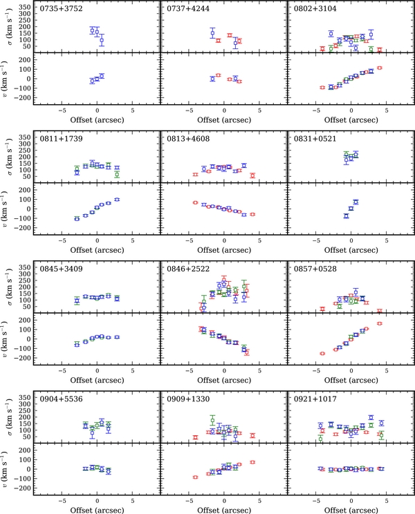
Figure 2. Same as Figure 1. 0737+4244, 0857+0528, and 0904+5536 have AGN contamination of the central measurement(s). 0737+4244 also has AGN contamination of the central CaT measurement. 0811+1739, 0831+0521, 0845+3409, and 0904+5536 lack CaT data due to instrument problems.
Download figure:
Standard image High-resolution image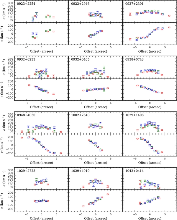
Figure 3. Same as Figure 1. 0923+2254 inner measurements from all regions are excluded due to AGN contamination.
Download figure:
Standard image High-resolution image
Figure 4. Same as Figure 1. 1049+2451 has AGN contamination of the central CaHK and CaT measurement(s). 1147+0902 has AGN contamination in central CaHK measurements. 1143+5941 and 1145+5547 lack CaT data due to instrument problems.
Download figure:
Standard image High-resolution image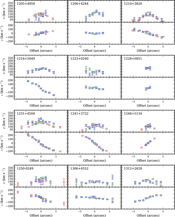
Figure 5. Same as Figure 1. 1312+2628 has AGN contamination in central CaHK measurements. 1206+4244, 1216+5049, 1223+0240, 1228+0951, 1306+4552, and 1312+2628 lack CaT data due to instrument problems.
Download figure:
Standard image High-resolution image
Figure 6. Same as Figure 1. 1535+5754 has AGN contamination in central CaHK and MgIb measurements. 1313+3653, 1353+3951, 1416+0137, 1423+2720, and 1543+3631 lack CaT data due to instrument problems.
Download figure:
Standard image High-resolution image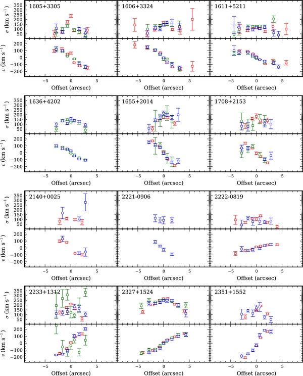
Figure 7. Same as Figure 1. 1605+3305, 1708+2153, 2140+0025, 2222−0819, and 2233+1312 have AGN contamination in central measurements. MgIb measurements are excluded for 2140+0025, 2221−0906, and 2222−0819 due to insufficient wavelength coverage (redshift). 1636+4204 lacks CaT data due to instrument problems. The 2140+0025 central measurement is affected by telluric lines for all regions.
Download figure:
Standard image High-resolution image
Download figure:
Standard image High-resolution image
Figure 8. Aperture stellar velocity dispersions from the CaT region (red), MgIb region (green), and CaHK region (blue), in km s−1. CaHK and CaT measurements are excluded when contaminated by AGN emission. MgIb measurements are absent in cases of narrow wavelength coverage (redshift). These exclusions mirror those of Figures 1–7.
Download figure:
Standard image High-resolution imageTable 2. σ Measurements
| Target | S/N | σSDSS | σbest |
|---|---|---|---|
| (pixel−1) | (km s−1) | (km s−1) | |
| (1) | (2) | (3) | (4) |
| 0013−0951 | 68.4 | 134 ± 5 | 134 ± 5 |
| 0026+0009 | 152.8 | 170 ± 2 | 170 ± 2 |
| 0038+0034 | 57.8 | 131 ± 6 | 131 ± 6 |
| 0109+0059 | 38.8 | 165 ± 17a | 165 ± 17 |
| 0121−0102 | 79.0 | 107 ± 11 | 107 ± 11 |
| 0150+0057 | 82.2 | 193 ± 4 | 193 ± 4 |
| 0206−0017 | 132.8 | 218 ± 6 | 218 ± 6 |
| 0212+1406 | 107.1 | 188 ± 4 | 188 ± 4 |
| 0301+0110 | 79.5 | 97 ± 4 | 97 ± 4 |
| 0301+0115 | 80.2 | 90 ± 6 | 90 ± 6 |
| 0336−0706 | 124.1 | 246 ± 3 | 246 ± 3 |
| 0353−0623 | 45.5 | 196 ± 11 | 196 ± 11 |
| 0735+3752 | 16.1 | 156 ± 23a | 156 ± 23 |
| 0737+4244 | 10.2 | 90 ± 18c* | 90 ± 18 |
| 0802+3104 | 82.4 | 113 ± 4 | 113 ± 4 |
| 0811+1739 | 89.6 | 136 ± 6a | 136 ± 6 |
| 0813+4608 | 101.2 | 120 ± 4 | 120 ± 4 |
| 0831+0521 | 36.2 | 201 ± 13a | 201 ± 13 |
| 0845+3409 | 103.1 | 121 ± 5a | 121 ± 5 |
| 0846+2522 | 96.1 | 251 ± 12 | 251 ± 12 |
| 0857+0528 | 81.2 | 127 ± 5 | 127 ± 5 |
| 0904+5536 | 59.8 | 132 ± 8b | 128 ± 9 |
| 0909+1330 | 51.5 | 91 ± 5 | 91 ± 5 |
| 0921+1017 | 79.6 | 98 ± 3 | 98 ± 3 |
| 0923+2254 | 40.8 | 129 ± 6c* | 129 ± 6 |
| 0923+2946 | 75.5 | 143 ± 3 | 143 ± 3 |
| 0927+2301 | 144.8 | 195 ± 2 | 195 ± 2 |
| 0932+0233 | 55.1 | 124 ± 4 | 124 ± 4 |
| 0932+0405 | 62.7 | 96 ± 6 | 96 ± 6 |
| 0938+0743 | 110.4 | 124 ± 3 | 124 ± 3 |
| 0948+4030 | 110.5 | 140 ± 3 | 140 ± 3 |
| 1002+2648 | 74.4 | 154 ± 8 | 154 ± 8 |
| 1029+1408 | 93.4 | 197 ± 5 | 197 ± 5 |
| 1029+2728 | 70.7 | 127 ± 6 | 127 ± 6 |
| 1029+4019 | 74.1 | 165 ± 6 | 165 ± 6 |
| 1042+0414 | 59.8 | 108 ± 10a | 108 ± 10 |
| 1049+2451 | 60.3 | 80 ± 17b | 77 ± 17 |
| 1058+5259 | 67.5 | 121 ± 3 | 121 ± 3 |
| 1101+1102 | 42.1 | 144 ± 14 | 144 ± 14 |
| 1104+4334 | 65.7 | 91 ± 7 | 91 ± 7 |
| 1116+4123 | 68.2 | 131 ± 4 | 131 ± 4 |
| 1118+2827 | 66.8 | 119 ± 3 | 119 ± 3 |
| 1137+4826 | 55.9 | 166 ± 7 | 166 ± 7 |
| 1140+2307 | 82.3 | 82 ± 2 | 82 ± 2 |
| 1143+5941 | 105.8 | 121 ± 6a | 121 ± 6 |
| 1144+3653 | 64.8 | 160 ± 8b | 155 ± 8 |
| 1145+5547 | 94.5 | 118 ± 6a | 118 ± 6 |
| 1147+0902 | 98.8 | 113 ± 15b | 120 ± 18 |
| 1205+4959 | 81.5 | 166 ± 6 | 166 ± 6 |
| 1206+4244 | 80.6 | 162 ± 5b | 157 ± 6 |
| 1210+3820 | 135.3 | 144 ± 5 | 144 ± 5 |
| 1216+5049 | 85.2 | 172 ± 7a | 172 ± 7 |
| 1223+0240 | 106.4 | 100 ± 7b | 97 ± 8 |
| 1228+0951 | 40.8 | 184 ± 10a | 184 ± 10 |
| 1231+4504 | 84.8 | 228 ± 7a | 228 ± 7 |
| 1241+3722 | 92.7 | 144 ± 4 | 144 ± 4 |
| 1246+5134 | 52.0 | 113 ± 5 | 113 ± 5 |
| 1250−0249 | 44.3 | 107 ± 8 | 107 ± 8 |
| 1306+4552 | 89.8 | 100 ± 4a | 100 ± 4 |
| 1312+2628 | 141.4 | 125 ± 5b | 133 ± 9 |
| 1313+3653 | 37.2 | 183 ± 24a | 183 ± 24 |
| 1323+2701 | 32.0 | 122 ± 9 | 122 ± 9 |
| 1353+3951 | 44.0 | 168 ± 11a | 168 ± 11 |
| 1405−0259 | 67.2 | 123 ± 4 | 123 ± 4 |
| 1416+0137 | 96.0 | 149 ± 4a | 149 ± 4 |
| 1419+0754 | 79.7 | 185 ± 10 | 185 ± 10 |
| 1423+2720 | 49.8 | 128 ± 7a | 128 ± 7 |
| 1434+4839 | 58.9 | 114 ± 7 | 114 ± 7 |
| 1535+5754 | 179.5 | 116 ± 4 | 116 ± 4 |
| 1543+3631 | 65.2 | 119 ± 9a | 119 ± 9 |
| 1545+1709 | 94.0 | 171 ± 5 | 171 ± 5 |
| 1554+3238 | 97.9 | 159 ± 4 | 159 ± 4 |
| 1605+3305 | 90.9 | 186 ± 8 | 186 ± 8 |
| 1606+3324 | 64.4 | 170 ± 8 | 170 ± 8 |
| 1611+5211 | 92.9 | 120 ± 5 | 120 ± 5 |
| 1636+4202 | 84.8 | 144 ± 10a | 144 ± 10 |
| 1655+2014 | 59.9 | 199 ± 6 | 199 ± 6 |
| 1708+2153 | 92.6 | 172 ± 13 | 172 ± 13 |
| 2140+0025 | 12.2 | 71 ± 28c* | 71 ± 28 |
| 2221−0906 | 33.9 | 115 ± 17a | 115 ± 17 |
| 2222−0819 | 79.9 | 99 ± 8 | 99 ± 8 |
| 2233+1312 | 78.2 | 198 ± 6 | 198 ± 6 |
| 2327+1524 | 142.8 | 266 ± 3 | 266 ± 3 |
| 2351+1552 | 73.3 | 237 ± 9 | 237 ± 9 |
Notes. Reference σ measurements for the objects in our sample from which at least one σ measurement could be obtained.
aFrom CaHK;
bfrom MgIb;
c*from spatially resolved spectrum; farther than 05 from the Sloan radius.
Column 2: S/N per pixel is calculated from rest-frame 8480–8690 Å (5050–5450 Å if measurement is from CaHK or MgIb).
Column 3: Our best raw measurement at the Sloan fiber radius. Here if CaT could not be used, we report CaHK; if CaHK was also unavailable, we report MgIb. If AGN contamination contaminated all aperture spectra, we use the spatially resolved spectrum closest to 15 with the same regional preference. The result of this selection is noted by the superscripts.
Column 4: our best measurement of σ for the target, with wavelength range bias correction (from Section 5) and regional bias correction (from Section 6) applied. Note that if the raw measurement came from spatially resolved spectra, we apply the corrections derived from spatially resolved spectra; otherwise we use aperture corrections.
The data were reduced using Python-based scripts that include the standard reduction steps such as bias subtraction, flat fielding, and cosmic-ray rejection. Arclamps were used for wavelength calibration in the blue and sky emission lines in the red. A0V Hipparcos were used to correct for telluric absorption and to perform relative flux calibration; to minimize overhead, these stars were observed immediately after a group of objects close in coordinates.
Throughout this paper, we use S/N (pixel−1) as a measurement of spectrum quality, particularly the quality of absorption features. Therefore in our determination of S/N we use the same (or similar) wavelength ranges used for stellar velocity dispersion fitting (see Section 4)—5050–5450 Å in the blue and 8480–8690 Å in the red. The blue chip physically ends around 5600 Å, so many spectra do not actually extend to 5450 Å (in which case we use 5050 Å to the end of the spectrum). We determine the S/N from spectra before Fe ii subtraction (Section 3.3) so for objects with strong Fe ii emission the blue S/N does not necessarily reflect absorption line quality, but should be a good estimator for the Fe ii-subtracted spectra used for the fit.
We caution the reader that our higher-offset measurements of S/N and σ may be biased for late-type galaxies with bright star-forming regions, because we align the slit with the host galaxy major axis (which contains, when present, the galaxy's bright spiral arms). In these cases, the S/N is increased by the young stars to a level that does not accurately reflect the older stellar populations that are of interest to our study. These younger stars may also bias our measurements of σ, although our fitting procedure can incorporate young stellar templates when needed (Section 4).
3.2. Extraction of One-dimensional Spectra: Aperture versus Spatially Resolved Spectra
From the reduced two-dimensional spectra, one-dimensional spectra were extracted either as "spatially resolved" spectra or "aperture" spectra in the following manner.
"Spatially resolved" spectra were created to measure the variation of σ as a function of radius. We extracted a central spectrum with a width of 054 (043) in the blue (red) for nights before 2009 September but a width of 054 in both the blue and red for 2009 September onward (i.e., after the red CCD chip upgrade). Off-center spectra were extracted by stepping out from the center in both directions, at every step increasing the extraction window by 1 pixel (above and below the trace) and choosing the step size such that there is no overlap with the extraction window of the previous step.
Spatially resolved spectra do not represent the way in which most studies extract one-dimensional spectra from which to measure σ. Instead, one-dimensional spectra are usually created from a broad extraction window centered on the galactic center. In the following, we refer to a spectrum created in such a way as an "aperture spectrum." If made from a two-dimensional spectrum, the width of the extraction window is chosen according to some criterion, e.g., to obtain a certain S/N. However, fiber spectra such as SDSS spectra come from a fixed circular aperture of 3'' diameter.
Our study is concerned with the effect of the width of the extraction window on σ when creating aperture spectra. Therefore, in addition to the spatially resolved spectra, we create a series of aperture spectra of increasing aperture width, ranging from ∼05 to ∼7'' in 027 increments (26 spectra per object). With this range of aperture widths we can not only study the effect of increasing aperture width on σ but also directly compare our measurements to measurements in the literature and to the results that would be derived from Sloan fiber spectra. For the latter, we determine σap, SDSS, measured from aperture spectra within the central 15 radius as a proxy for what would have been measured with the 3'' diameter Sloan fiber. Note, however, that in fact, our σap, SDSS corresponds to a rectangular region of dimension 3'' by 1'' given the width of the long slit.
With both types of extraction we can test whether the agreement between the three different spectral regions used to determine σ depends on offset from galactic center or aperture width (Section 6).
3.3. Subtraction of Fe ii Pseudocontinuum Emission
The majority of objects (58 out of the 96 in the spectroscopic sample) display broad nuclear Fe ii emission in their spectra (∼5150–5350 Å) that interferes with σ measurements from the MgIb region. For those objects, we simultaneously fit a set of IZw1 templates (varying width and strength) and a featureless AGN continuum to the central (spatially resolved) spectrum. The best fit was determined by minimizing χ2 and was then subtracted from the five central offset positions in spatially resolved spectra, and from all aperture spectra. Fe ii-corrected spectra were not used in the CaHK measurements, since Fe ii features in this region are too broad and weak to have an effect on σ (Greene & Ho 2006b). Fe ii subtraction is illustrated in Figures 2 and 3 of Paper I, and details can be found in Woo et al. (2006).
4. STELLAR VELOCITY DISPERSION FITTING
4.1. Overview of the Fitting Code
Here, we present a brief overview of our fitting method. Tests of the method are provided in the Appendix.
As described in Section 5.2 of Suyu et al. (2010), we use a Python-based code that employs the algorithm of van der Marel (1994) but expanded to use a linear combination of template spectra. The code simultaneously fits a linear combination of broadened stellar templates and a polynomial continuum to the data, using a Markov Chain Monte Carlo (MCMC) routine to find the best-fit velocity dispersion (σ) and velocity (v). The stellar template library is composed of seven G and K giants of various temperatures as well as spectra of A0 and F2 giants from the Indo-US survey. Before fitting, template spectra are rebinned to the instrumental resolution determined from the science spectrum. Our reported measurement of σ (or v) is the median of the MCMC distribution, and measurement errors are the semi-difference of the values at the 16 and 84 percentile values (see the Appendix for a discussion of the relative merits of the median, mean, and most likely values as estimates). Systematic errors due to template variations are accounted for in our fitting routine since the template weights are fitted simultaneously with the velocity dispersion and marginalized over.
Our fitting routine employs Gaussian broadening kernels (range 30–500 km s−1) to the templates. This is the standard quantity measured for the host galaxy of black holes and it is therefore the quantity that needs to be measured in order to compare our results with the previous literature (e.g., Ferrarese & Merritt 2000; Barth et al. 2002; Onken et al. 2004; Greene & Ho 2006a; Gültekin et al. 2009; Woo et al. 2010). We should note, however, that line profiles are not necessarily Gaussian and a more accurate determination of σ can be obtained by relaxing this assumption (see, e.g., van der Marel & Franx 1993). This is left for future work.
4.2. Determination of Fit Parameters
For each measurement we need to set a few parameters. These determine whether A and F stars are required, set the wavelength range to fit, and define masks and the order of the continuum fit. We now discuss how we determine each of these parameters from the spatially resolved spectra and how we apply them to the aperture spectra.
Every fit is initially performed with all seven G and K stellar templates, without the A0 and F2 templates. Some spectra show strong Hδ absorption in one or more of the noncentral spatially resolved spectra (presumably due to a region of star formation) and therefore could not be fit well by G and K templates alone. In these cases, the A and F stellar templates are also included in the fitting procedure for both the spatially resolved and aperture σ measurements.
As anticipated in Section 3.1, to test the dependency of stellar velocity dispersion on observed spectral regions we independently fit to three different regions corresponding to commonly used deep stellar absorption features: (1) around the Ca ii NIR triplet, 8480–8690 Å (CaT), (2) around the Mg Ib triplet, 5050–5330 Å (MgIb), and (3) around Ca H&K, 3910–4300 Å.
In region (1), if the broad AGN emission line O i λ8446 is present and superposed with the first of the CaT lines, we exclude the first CaT line and used 8520–8690 Å. In some cases, imperfect subtraction of telluric absorption lines or cosmic rays requires that the third line be excluded. Thus, σCaT may be determined from all three lines, the second and third lines, the second and first lines, or the second line alone. In region (2), though the longest rest-frame wavelength used is 5330 Å, the wavelength range available for a given object depends on its redshift, as the spectra end at the observed wavelength 5600 Å. At z ≳ 0.08, there is not enough information in the MgIb region to recover σ. In region (3), if the H AGN emission line filled the CaH stellar absorption line, we exclude the Ca H&K lines and instead use only weaker absorption features in the range 4150–4300 Å. For all but two objects, excluding Ca H&K lines was necessary for the central three spatially resolved spectra. The effect of these wavelength range variations on σ is discussed in Section 5.
Note that the G-band feature redward of 4300 Å that usually provides a good measure of galaxy kinematics is excluded from the CaHK region, to avoid the broad Hγ λ4341 emission feature.
Within the chosen region, we apply masks to ensure that we fit only the stellar contributions to each spectrum. In the blue regions, we check for narrow AGN emission features such as [Fe v] λ4227.49; [Fe vi] λλλ5145.77, 5176.43, 5335.23; [Fe vii] λλ5158.98, 5277.67; [N i] λλ5197.94,5200.41; [Ca v] λ5309.18 (wavelengths taken from Moore 1945; Bowen 1960), and various broad He i and Balmer lines. In the red, we may mask wavelength ranges that are affected by telluric absorption rather than shorten the region, if the affected range is narrow or does not extend to the end of the spectrum. In any case, a mask is only applied to known contaminating features when doing so changes the measurement more than the uncertainty on the original measurement.
As for the order of the polynomial continuum, we choose the lowest order that preserves the quality of the fit; most commonly, this is a linear continuum (i.e., a first-order polynomial). However, in the bluest regions, AGN emission features at either end of the wavelength range or sudden continuum breaks (e.g., near the Ca H&K feature) require the use of a third-order polynomial (or second-order, in a few cases).
Each of these parameters (template set, wavelength range, masks, polynomial order) is determined by visual inspection of each spatially resolved spectrum with an S/N ≳ 10 pixel−1. In effect, this S/N restriction is a restriction on the maximum offset observed, as S/N decreases as a function of offset (galaxies are dimmer at larger radii). Every spatially resolved spectrum must be inspected because the contribution of the AGN changes with offset in a unique way for every target. Additionally, noise features such as bad pixels or cosmic-ray subtraction residuals affect only certain offsets.
It is infeasible to apply this same vigilance to the aperture spectra because we make nearly 100 aperture σ measurements per object. Furthermore, there is a physical reason to expect that such vigilance is unnecessary, since these parameters depend predominantly on AGN emission features, which are shared among all aperture spectra. We therefore expect that the central fit parameters determined from the spatially resolved spectra are sufficient for all aperture spectra, so we apply the parameters determined from an object's central spatially resolved spectrum to all of its aperture spectra.
However, our treatment of the aperture fits is not completely blind. We visually inspect the aperture spectra at the Sloan fiber radius for all measurements. Additionally, if A and F templates were required for any spatially resolved measurements, then we also apply these templates to the aperture spectra that would be similarly affected, i.e., aperture widths greater than or equal to the offset position of the spatially resolved spectra in which the Hδ absorption feature is observed. In some cases the aperture spectra include noise features not seen in the spatially resolved spectra, because the aperture spectra cover a larger spatial extent than the spatially resolved spectra due to S/N constraints on the spatially resolved spectra discussed above. In such cases we visually inspect the target's widest aperture spectrum to determine the mask for all aperture spectra.
4.3. Results: Stellar Velocity Dispersion Measurements
The resulting σ for all objects are provided here in Figures 1–7 (spatially resolved) and Figure 8 (aperture). Examples of our spectral fits are provided in Figures 4–7 of Paper I and will not be repeated here for conciseness. No corrections (e.g., for wavelength range used, Section 5) have been applied to these measurements. As mentioned in Section 4.1, our code determines the v required to precisely align the templates with the rest-frame spectra (a minor correction to the Sloan redshift), which we use to determine systemic velocities, shown in the lower panels (relative to 〈v〉). We also plot the velocity dispersion and velocity profiles for all the objects analyzed in Paper I for completeness; the measurements presented here supersede those given in Paper I.
As noted in Paper I, in Figures 1–7, measurement errors tend to be larger for spectra with low S/N (i.e., higher offsets) as well as—for CaHK and MgIb—spectra with higher AGN contribution (i.e., central offsets). In many cases central CaHK measurements (blue points) are missing since σCaHK could not be faithfully determined due to AGN contamination; in some cases, the AGN predominance also requires the exclusion of central σMgIb and σCaT measurements. Note also that σMgIb may be missing from the objects with highest redshift because the 5600 Å instrumental limit did not leave strong enough features for a measurement of σMgIb, and objects observed on 2010 March 14 do not have σCaT due to problems at the instrument.
Without the photometric determination of the spheroid effective radius, we can only make a few qualitative and general comments about σ spatial profiles from Figures 1–8. From the spatially resolved profiles, we see that in all regions σ tends to either decrease with increasing offset or remain relatively constant. We see that higher concavity in these profiles correlates with a higher slope in the rotation curve, i.e., σ decreases more rapidly with offset from the center in galaxies with strong rotational signatures. In the aperture profiles, we see that profiles are relatively flat, having in general small variations compared to those seen in the spatially resolved dispersions. These conclusions are qualitative estimations of the results we expect to see when photometry is incorporated (Paper III), constraining the spheroid effective radius (reff, sph). We can then plot the dispersion profiles in units of reff, sph to make more meaningful comparisons between the galaxies, and to have a physical benchmark for quantitative analysis of trends in the σ profiles.
Finally, we provide the results of our fits to the aperture spectra at the Sloan fiber radius in Table 2, along with the S/N per pixel of the spectrum. Column 3 of this table lists measurements without any corrections applied, from the CaT region. If we could not fit to the CaT region we provide the measurement from the MgIb or CaHK region, again at the Sloan fiber radius. If we were not able to fit to any aperture spectra—due to AGN contamination—we provide the spatially resolved measurement closest to the Sloan fiber radius. Column 4 of this table provides our best measurement of σ, which takes the result of Column 3 and applies the corrections for both wavelength range and spectroscopic region found in Sections 5 and 6. Note that by "best" we refer to the best measurement we can deduce without photometric results. With reff, sph we will be able to calculate a luminosity-weighted σ that removes the effect of the disk, as in Paper I, which we consider to be a more accurate σ.
As discussed in Section 1, we consider 10% to be the upper limit on the desired accuracy of σ measurements, but 5% is our goal. Our σbest have an average error of 5.9% ± 0.6% and median error of just 4.5%. Of the 84 σ, 9 have errors higher than 10% but come from the lower-quality spectra (mean S/N of 43 pixel−1 compared to the mean of the total sample, 78 pixel−1).
All the measurements shown in Figures 1–7 are provided in Table 3
Table 3. Spatially Resolved σ Measurements
| Object | Red Offset | σCaT | Blue Offset | σMgIb | σCaHK |
|---|---|---|---|---|---|
| (arcsec) | (km s−1) | (arcsec) | (km s−1) | (km s−1) | |
| (1) | (2) | (3) | (4) | (5) | (6) |
| 0026+0009 | 0.00 | 158.61 ± 3.05 | 0.00 | 186.05 ± 4.90 | 195.28 ± 6.73 |
| 0026+0009 | −0.81 | 144.52 ± 3.28 | −0.68 | 182.47 ± 6.62 | 158.73 ± 9.13 |
| 0026+0009 | +0.81 | 168.17 ± 3.31 | +0.68 | 199.82 ± 6.00 | 166.99 ± 8.49 |
| 0026+0009 | −2.16 | 112.44 ± 3.74 | −1.62 | 149.17 ± 10.52 | 149.13 ± 7.42 |
| 0026+0009 | +2.16 | 123.09 ± 3.44 | +1.62 | 175.95 ± 9.36 | 150.34 ± 6.55 |
| 0026+0009 | −4.05 | 82.16 ± 5.82 | −2.84 | 103.68 ± 13.53 | 99.04 ± 8.19 |
| 0026+0009 | +4.05 | 81.98 ± 5.13 | +2.84 | 113.64 ± 10.41 | 113.88 ± 6.04 |
| 0026+0009 | ... | ... | −4.32 | 65.85 ± 9.93 | 75.24 ± 12.52 |
| 0026+0009 | ... | ... | +4.32 | 87.45 ± 15.36 | 78.05 ± 10.00 |
Notes. Column 1: target ID. Column 2: red chip offset of spatially resolved spectrum from center. Column 3: derived σ in (km s−1) from the CaT region. Column 4: blue chip offset of spatially resolved spectrum from center. Column 6: same as Column 3 for CaHK region. Column 8: same as Column 3 for MgIb region.
Only a portion of this table is shown here to demonstrate its form and content. A machine-readable version of the full table is available.
Download table as: DataTypeset image
5. FIDELITY OF σ MEASUREMENTS AS A FUNCTION OF WAVELENGTH RANGE
As anticipated in Section 4.2, it is often necessary to exclude one or more (possibly all) of the strong stellar absorption lines in a given spectral region. This may be due to contamination by AGN emission features, the difficulty of correcting for telluric absorption, the presence of strong sky emission lines, or the challenges of removing instrumental defects from the data. Another potential reason for excluding a certain part of the spectral range is mismatch in element abundance ratios between template stellar spectra and galaxy spectra. An example of this effect is enhanced Mg/Fe abundance in massive early-type galaxies compared to typical galactic stars. This is discussed in detail by Barth et al. (2002) and will not be repeated here. In this section, for each spectral region we compare measurements from the full (ideal) wavelength range to measurements from common narrower wavelength ranges including those narrower ranges used in this paper.
For the analysis of this section and Section 6, we experimented with different procedures to compute averages (μ) and their uncertainties (δμ). As our default we use a Bayesian estimator that assumes a Gaussian distribution with intrinsic scatter (Δ) as a free parameter and takes into account the uncertainty associated with each measurement. The μ reported is the median of the distribution, and δμ is the semi-difference of the 16 and 84 percentile values. In order to minimize the effects of potential outliers that may skew the Bayesian estimator, we apply 4-Δ clipping in an iterative scheme for data with high intrinsic scatter (Section 6 only). Alternative schemes like straight average, weighted average, or maximum likelihood estimators result in differences of order 0.01 dex in the best estimate, which we accounted for by adding a systematic uncertainty term to our measurements.
5.1. CaT Region
Although the CaT region is generally considered the best region for measuring σ—for active galaxies in particular, due to the scarcity of AGN emission features in this wavelength range—it nevertheless can be affected by AGN contamination or, at higher redshifts, by telluric absorption. A typical situation occurs when one has to exclude the bluest and reddest lines of the triplet (hereafter, first and third, respectively); the first line may need to be excluded due to O i contamination and the third line may need to be excluded when it is redshifted into strong telluric features.
Unlike the CaHK and MgIb regions discussed below, the CaT region does not have nearby (strong) absorption lines from which we can measure σ. Measurements rely on the Ca ii triplet lines alone. Therefore we test the effect of line exclusion, making independent measurements of σ using various wavelength ranges in the CaT region. For brevity we denote the velocity dispersions measured using the first and second lines (8480–8580 Å), the second line alone (8520–8580 Å), and the second and third lines (8520–8690 Å) as σ1, 2, σ2, and σ2, 3, respectively. We refer to these generically as σcut, and our diagnostic for agreement is log (σcut/σ).
It may be that σcut/σ is a function of AGN contamination (i.e., spatial offset) or S/N—or a combination of the two—so we study σcut/σ as a function of each. An illustrative example of our results is the top panel of Figure 9 (errors are statistical only, i.e., without our 0.01 dex systematic uncertainty).
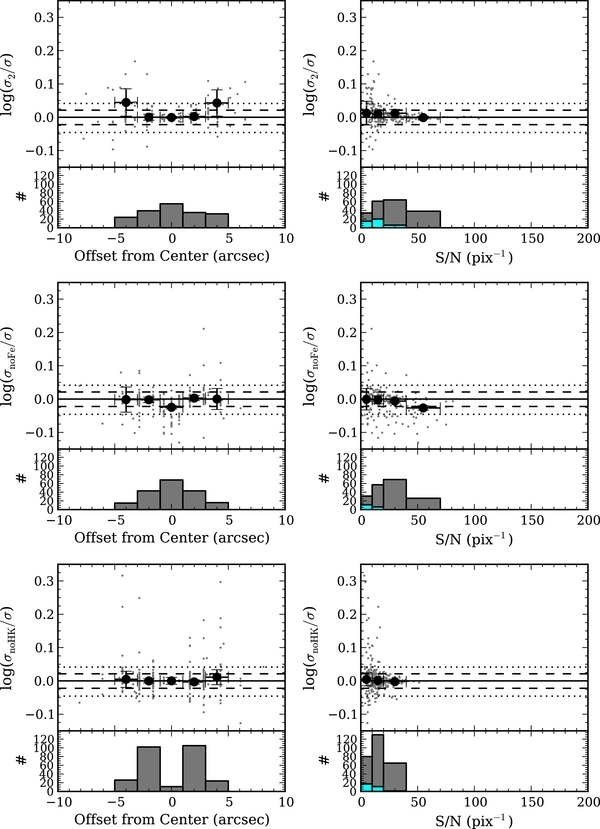
Figure 9. Comparison of σ from the different regions when we shorten the wavelength range of a region. Top row: σCaT from 8480 to 8580 Å (i.e., excluding the third line; σ1, 2); middle: σMgIb from 5050 to 5250 Å (i.e., excluding Fe λ5270; σnoFe); bottom: σCaHK from 4150 to 4300 Å (i.e., excluding Ca H&K; σnoHK). Left column: plotted against offset position; right: plotted against S/N. Black circles represent the average value and error bars are the error on the mean; gray points are individual measurements to give an estimate of intrinsic scatter; bins with fewer than ten points are omitted. For reference, we plot 5% (our target accuracy; dashed lines) and 10% difference (dotted lines). Cyan bars in the histograms (S/N plots only) show the number of measurements from an offset >3'' from the center—higher offsets have S/N< 20 pixel−1, so apparent trends with offset reflect S/N trends.
Download figure:
Standard image High-resolution imageWe find no trends with offset or S/N. As expected, scatter greatly increases at S/N <20 pixel−1. As illustrated by the cyan bars in the right panel of Figure 9, high-offset spectra are dominated by low-S/N trends. As described in the Appendix, independent of σ, measurements are most reliable for S/N⩾20 pixel−1 and we therefore impose this requirement on the measurements used to calculate biases. From the high S/N measurements (108 of 203), we find no bias in any of the three most common cases: 〈log (σ1, 2/σ)〉 = 0.001 ± 0.003 ± 0.01, 〈log (σ2/σ)〉 = 0.001 ± 0.003 ± 0.01, and 〈log (σ2, 3/σ)〉 = 0.002 ± 0.003 ± 0.01.
Of particular importance is our finding that σ2 recovers σ measured from the full CaT region accurately. As we see in Figure 9, the recovery is perfect with extremely low (≈1%) statistical dispersion. At "intermediate" S/N (10 pixel−1 < S/N <40 pixel−1) σ2 is only ≈2.5% higher than σ, that is, equal within the 2.5% statistical dispersion.
This is a critical result for studies of the MBH–σ relation because it broadens the candidate pool for target selection, especially at higher redshifts where the third line is blanketed by telluric features. As an illustrative example, when compiling their target sample Greene & Ho (2006a) required that at least two of the three Ca ii IR lines be available; but we show that this two-line constraint is not necessary. Had the two-line constraint been removed from the Greene & Ho (2006a) sample selection process, the study may have been able to use a greater number of high-S/N spectra, increasing both its sample size and data quality.
5.2. MgIb Region
Our default wavelength range for the MgIb region is 5050–5330 Å, though redshift may truncate the red end. To investigate potential systematics due to excluding parts of the region, we study the effect of measuring σ from 5050 to 5250 Å and 5100 to 5330 Å. The first choice is motivated by redshift—to avoid atmospheric contamination, we set the dichroic to 5600 Å (observed) and therefore could not recover the full range for z ≳ 0.051. Because it excludes the Fe λ5270 absorption feature, we refer to this range as σnoFe. The second choice is motivated by contamination from AGN emission—the red wing of [O iii]λ5007 or other AGN emission features such as He iλ5016,5048 may contaminate the blue end of the MgIb region. Because it represents the red end of the MgIb region, we refer to this range as σMgred. Our results for σnoFe are illustrated in the middle row of Figure 9. These comparisons were made only among objects for which the full region was available.
In both cases, we find no strong trend with S/N. However, interestingly, the central spectra give different results from the higher-offset spectra. We report only 〈log (σnoFe/σ)〉 because—regardless of offset—it is equal to 〈log (σMgred/σ)〉. Averaging over measurements with S/N >20 pixel−1 (100 of 188 measurements), we find 〈log (σnoFe/σ)〉 = −0.016 ± 0.004 ± 0.01.
Since there are clear spatial trends we analyze different offsets separately (still requiring S/N >20 pixel−1). Central spectra (22 measurements) give 〈log (σnoFe/σ)〉 = −0.04 ± 0.01 ± 0.01 and spectra within 07 (42 measurements) give 〈log (σnoFe/σ)〉 = −0.0191 ± 0.006 ± 0.01 and non-central spectra (36 measurements) give 〈log (σnoFe/σ)〉 = 0.001 ± 0.007 ± 0.01.
The small bias in σnoFe is in the same direction as that reported by Barth et al. (2002) who noticed that including Mg (or, in our case, increasing its significance by eliminating Fe) can bias σ high at the 5% level (10% for central measurements). This bias is mass-dependent, so we note that our mass range (or, equivalently, stellar velocity dispersion range) is similar to the Barth et al. (2002) sample (see Section 6.3 and Figure 11). We thus recommend that measurements based on spectral ranges that are dominated by Mg i be corrected by multiplying by 1.05 ± 0.03 if they cannot be avoided.
5.3. CaHK Region
Our default wavelength range for the CaHK region is 3910–4300 Å. If strong H fills the Ca H feature we use 4150–4300 Å, excluding both the Ca H and K features (σ measured from this range is named σnoHK). The standard region includes the Hδ feature, which might be biased by the presence of thermally broadened absorption from A and F stars if those are not properly represented in the templates. Thus, we also test a third region that excludes the Hδ but includes Ca H&K (3900–4090 Å; σ measured from this range is named σnoHδ). This is approximately the wavelength range used in Greene & Ho (2006a). As always, these tests are only run for spectra with available Ca H. Our results for σnoHK are illustrated in the bottom row of Figure 9.
Similarly to the case for CaT, the narrower wavelength ranges accurately recover the same σ as the full range, though dispersion increases greatly for S/N < 20 pixel−1. Using measurements with S/N >20 pixel−1 (68 of 278 measurements), 〈log (σnoHK/σ)〉 = −0.002 ± 0.005± 0.01 and 〈log (σnoHδ/σ)〉 = −0.002 ± 0.005 ± 0.01, corresponding to no bias for either.
5.4. Summary of Results
We find that reducing the size of the wavelength range does not affect σCaT or σCaHK although it decreases marginally σMgIb, seemingly as a function of AGN contribution. Our results in the MgIb region confirm and strengthen the findings by Barth et al. (2002), showing that excluding the Fe lines in the MgIb region lowers σ by 5% ± 3%.
For our study of the fidelity of the CaHK and MgIb regions compared to CaT (Section 6), MgIb measurements are corrected for wavelength range bias according to the findings described in this section, and errors on these corrections are incorporated into the measurement error.
These findings have good implications for future studies: we consistently find that good data quality (high S/N) is the driving requirement for σ accuracy. Studies must understand the accuracy with which their fitting program recovers σ as a function of S/N; but provided spectra are above this S/N threshold, the unavoidable exclusion of strong lines due to telluric or AGN contamination does not affect results.
6. COMPARISON BETWEEN THE CaT, CaHK, AND MgIb REGIONS
As redshift increases, the CaT and MgIb regions are redshifted out of the optical wavelengths and measurements of σ may rely on the CaHK region exclusively. Therefore, it is necessary to understand systematic effects of measuring σ from the MgIb or CaHK region instead of the CaT region (see also Barth et al. 2002; Greene & Ho 2006a). We refer to these measurements, respectively, as σMgIb, σCaHK, and σCaT. We investigate the effects of S/N (Section 6.1), offset from center (or the aperture width; Section 6.2), and σ (Section 6.3). Blue-side σ are compared to the (spatially) closest σCaT, with the constraint that the two measurements be within 05 of each other (to avoid bias from the slopes of the σ spatial profiles, Figures 1–7).
6.1. Trends with S/N
We consider the effect of S/N before considering spatial effects, as the higher-offset spatially resolved spectra tend to fall in the lower S/N regime and therefore are affected by S/N trends, as seen in Section 5.
The desired S/N of a spectrum is a factor in determining exposure time and also the aperture width when extracting the spectra, so for higher-redshift studies that rely on the bluer regions, there is a strong motivation to know if σMgIb/σCaT or σCaHK/σCaT varies significantly with S/N. The concern is that there is an S/N threshold below which scatter is too high for a precise calibration of MgIb and CaHK to CaT.
We find no clear trends in 〈log (σCaHK/σCaT)〉 or 〈log (σMgIb/σCaT)〉 with S/N. As expected, scatter increases at S/N lower than 20 pixel−1 (see the Appendix).
6.2. Spatial Trends: Offset and Aperture Width
Having investigated possible trends with S/N and finding none, we now investigate whether σCaT/σCaHK or σCaT/σMgIb depend on the distance from the center or the aperture width, which are both affected by the AGN contribution in the center of the galaxy. A quantitative comparison of these measurements is shown in Figure 10. As in Section 5, for easy reference we draw dashed lines at 5% and 10% accuracy (5% accuracy is the target for this study). In this figure, if applicable, measurements have been corrected for the wavelength bias discussed in Section 5.
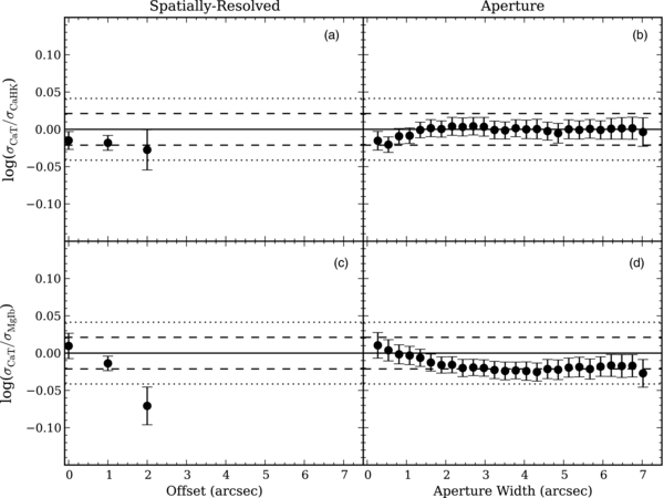
Figure 10. Comparison of σ measured from the CaHK region (top panels) and MgIb region (bottom panels) to the CaT region, as a function of distance from the center. Measurements are corrected for wavelength range bias, with error due to this correction incorporated. The mean is shown at each location, with the error on the mean. Bins with fewer than ten points are omitted. For quick reference we show 5% (dashed lines; target accuracy) and 10% lines (dotted lines).
Download figure:
Standard image High-resolution imageFor the spatially resolved analysis (panels (a) and (c)), measurements are put into 1'' bins (plotted at the center of the bin); bins containing less than 10 measurements are omitted because we expect our averaging procedure to underestimate the uncertainty in such cases. Note that for this analysis, the (arbitrary) sign of the spatial offset is disregarded, and 4-Δ clipping is used in each bin (see Section 5).
We find that 〈log (σCaHK/σCaT)〉 is constant within the errors, with values of −0.01 ± 0.01 ± 0.01 at 0'', −0.02 ± 0.01 ± 0.01 at 1'', and −0.03 ± 0.03 ± 0.01 at 2''. In contrast, 〈log (σMgIb/σCaT)〉 decreases marginally, dropping from 0.01 ± 0.02 ± 0.01 at 0'' to −0.019 ± 0.009 ± 0.01 at 1'' then −0.07 ± 0.03 ± 0.01 at 2''. In both cases, the 1'' bin contains the most measurements (≈85) while the 2'' contains the fewest (≈13) and the 0'' bin contains ≈35 measurements. These trends are qualitatively the same as were found in Paper I. In Section 5, we also found that MgIb results are somewhat more sensitive to offset than CaHK.
The aperture comparisons show that 〈log (σCaHK/σCaT)〉 and 〈log (σMgIb/σCaT)〉 are independent of aperture width by ∼25. The CaHK comparison (b) rises from its central value (same as spatially resolved central value) to a constant 0.00 ± 0.01 ± 0.01, and reaches this point by the Sloan fiber radius. The MgIb comparison (d) shows the same trend seen in the spatially resolved case: spectra with a higher fraction of galaxy light give a lower 〈log (σMgIb/σCaT)〉 than the central spectra. Here, the asymptotic value is −0.02 ± 0.01 ± 0.01.
With the spheroid effective radii for our objects we can revisit this spatial comparison in physical units, which may clarify the cause and strength of these trends.
In Table 2 and in Section 8, we use the results of this section to make σCaT-equivalent measurements from σCaHK and σMgIb.
6.3. Trends with Stellar Velocity Dispersion
Barth et al. (2002) investigated the fidelity of the MgIb region compared to the CaT region, although the MgIb wavelength range of those measurements extends from 5040–5430 Å, 100 Å greater in the red which may be significant as Greene & Ho (2006a) find 5250–5820 Å to be a superior measurement region.
Figure 11(a) mimics Figure 4 in the paper by Barth et al. (2002), comparing blue-side σ to σCaT as a function of σCaT(top panels). We use a linear plot here to show errors. Our data—σMgIb at the Sloan fiber radius, corrected for wavelength range bias—are plotted as filled circles and the Barth et al. (2002) data as open circles in panels (a) and (c). Barth et al. (2002) does not measure σCaHK so there is no data from that study in panels (b) and (d).
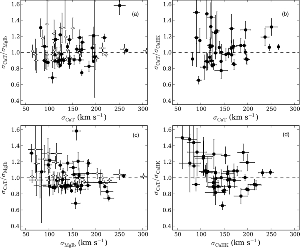
Figure 11. Comparison of σMgIb (left panels) and σCaHK (right panels) to σCaT, as a function σCaT (top panels) and σCaHK (bottom panels). Open circles are measurements from Barth et al. (2002), and filled circles are from this work. The distribution and average of our results agrees with that found in Barth et al. (2002). CaHK panels (b and d) contain only measurements from this work. All measurements from this work are corrected for wavelength range bias, including the associated uncertainty.
Download figure:
Standard image High-resolution imageOur sample and the Barth et al. (2002) sample have approximately the same distribution of measurements in both comparisons. The Barth et al. (2002) data return 〈log (σCaT/σMgIb)〉 = 0.003 ± 0.009, which agrees with our value (over all points, no S/N limits) of 0.00 ± 0.01. This agreement encourages an expansion upon the work presented in Barth et al. (2002) to the CaHK region, shown in Figure 11(b). As with MgIb, we see no clear trend with σCaT.
We also look for trends with blue-side σ (panels (c) and (d)), since the blue-side spectra have about half the kinematic resolution of the red and blue-side σ are generally considered to be less reliable. Plotting this way we see that most outlying measurements—measurements that are higher than the bulk of the measurements—occur at low σblue, in particular for σblue ≲ 125 km s−1, i.e., when we approach the resolution of the blue spectra. This is consistent with the limits of the fitting program, discussed in the Appendix.
6.4. Summary of Results
In this section, we explored the fidelity of the CaHK and MgIb regions compared to CaT. We made the comparison as a function of S/N, offset/aperture width, and σ.
S/N is a common diagnostic of spectrum quality. In the Appendix, we show that our fitting program is most reliable (independent of σ) at S/N above 20 pixel−1. Using only data above this threshold, we find no trends with S/N; below, scatter is high and trends are dominated by fitting complications.
Spatial offset and aperture width correlate with fraction of galaxy light in the spectrum. We find no significant spatial trend in σCaHK/σCaT, and for aperture widths greater than ≈1'', σCaHK is equal to σCaT. On the other hand, we find that σMgIb/σCaT decreases by about 10% between the 0'' and 2'' offsets; by an aperture width of ≈2'' 〈log (σMgIb/σCaT)〉 reaches its asymptotic of −0.02 ± 0.01 ± 0.01, a 5% ± 3% bias high in σMgIb.
Finally, we have made the comparison as a function of σ, following the MgIb analysis of Barth et al. (2002) who showed σMgIb/σCaT as a function of σCaT (note that study did not measure σCaHK). We see that the ratios are more strongly a function of the blue-side σ than σCaT; the data from both studies show that the scatter and value of σMgIb/σCaT and σCaHK/σCaT increase at low σ. We believe this trend reflects the limitations of fitting programs at σ close to the instrumental resolution (which is lower in the blue), as demonstrated in the Appendix.
Our analysis shows that σCaHK recovers σCaT faithfully, for sufficiently large S/N and velocity dispersion (see Appendix). However, even when the fitting program is in its most accurate regime, σMgIb is not equal to σCaT. In the central spectra, σMgIb is slightly lower than σCaT and in the highest offsets it is significantly higher.
7. AN OBSERVER'S GUIDE: HOW TO PREDICT THE SUCCESS RATE OF CaHK APERTURE SPECTRA FROM COLOR AND LOW-QUALITY SPECTRA
Since the CaT and MgIb regions are redshifted out of optical wavelengths first but lines in the CaHK region may be drowned by AGN emission features, future studies—especially of high-redshift targets—could benefit from a target selection guide to identify galaxies for which σ can be measured from the CaHK region.
In this section, we assume that future studies will be using aperture spectra, so a target is "unusable" in CaHK if its central spectrum is unreliable—our study may have a σCaHK from a higher offset. Reliability is determined by the visual inspection of the fit. As already exhaustively discussed in Sections 4.2 and 5, H often fills Ca H, and we can circumvent this contamination. The CaHK region is unreliable when the weaker features in the region are washed out by the neighboring Hγ and Hδ broad emission features. This reliable/unreliable classification therefore depends on AGN levels and to a minor extent on S/N.
There are "borderline" cases where it is not immediately clear that the features are too drowned by the AGN to be used; we are conservative and classify such cases as unreliable, because our goal is to build up a precise sample of σ measurements. Yet such cases serve to illustrate that this scheme of determining usability is subjective. It is difficult to make a more quantitative scheme, for instance by using stellar light fraction, because in unreliable cases the fitting program that would give us such meaningful values is, by definition, unable to reliably analyze the spectrum.
We have 33 of 96 objects in our spectroscopic sample from which we could not measure σCaHK reliably in aperture spectra due to high AGN emission levels. We ask if these 33 objects follow any trends in properties that could be estimated photometrically or from relatively low S/N and low-resolution spectra, such as those from SDSS. Colors and CaHK EW are a proxy for AGN contribution to the integrated spectrum and therefore we expect success rate to increase for redder colors and stronger CaHK absorption. We define "success rate" as Nreliable/Ntotal; we obtain this as a smooth function of each parameter by convolving our discrete points with a Gaussian broadening kernel.
In Figure 12, we evaluate the success rate as a function of g − r and u − g colors of each target (top left). The colors are extinction-corrected model magnitudes from SDSS-DR7. Given the low redshift of our targets, these colors are very close to the rest-frame colors and therefore can be used to guide selection of targets at any redshift based on multicolor photometry. Cyan points represent the targets contaminated by AGN emission in the central spectra. We see that these are indeed the bluest objects. The bottom left and top right panels show the success rate. Success rate drops below 50% for u − g < 0.7 and g − r < 0.5.

Figure 12. Guideline for target selection by color in order to get a reliable σ measurement. Colors taken from SDSS. Top left: g − r vs. u − g colors for all objects. Cyan points denote objects for which central measurements from CaHK were compromised by AGN emission. Top right: g − r vs. fraction of objects for which AGN emission did not contaminate central measurements of σ. Bottom left: fraction of objects for which AGN emission did not contaminate central measurements of σ vs. u − g.
Download figure:
Standard image High-resolution imageWe can also relate these limits to the amount of starlight versus AGNs in the galaxy by composite population synthesis. The tracks in Figure 12 show our calculations of AB colors at z = 0.076 for an old (12 Gyr; red, pentagons) and young (1 Gyr; blue, stars) stellar population with varying degrees of AGN contribution from 0% AGN (solid markers) to 100% AGNs, with open markers at 10% intervals along the tracks. For the older population, u − g > 0.7 and g − r > 0.5 correspond to roughly 85% stellar contribution (80% to meet the u − g limit, 90% for the g − r limit). The younger stellar population has g − r > 0.5 for stellar fractions above ≈65%, though u − g > 0.7 requires a stellar fraction of ≈80%. We see that in both cases the u − g constraint is—not surprisingly—the more limiting of the two, and for both the old and young stellar populations we find that a stellar fraction of ≳ 80% is required for a success rate greater than 50%.
In Figure 13, we study the success rate as a function of u − g and (EW) of the Ca H&K features in the aperture spectrum at the Sloan fiber radius (15); the panels are arranged as in Figure 12. We measure EW in the (rest-frame) wavelength range 3900–4020 Å according to

where f(λ) is the measured flux at λ and C(λ) is the approximated continuum level at λ. The rectangular approximation is good since Δλ is ≈0.5 Å, roughly 0.5% the width of the wavelength range. C(λ) is a line defined by the median flux within 3895–3905 Å (f3900) and 4015–4025 Å (f4020),
Positive EW corresponds to emission—in this case it translates to a very strong H emission feature dominating the Ca H&K absorption features.
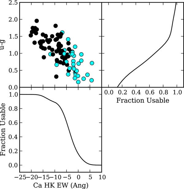
Figure 13. Guideline for target selection by u − g and equivalent width of the Ca H&K feature; equivalent width is measured from the aperture spectrum at the Sloan fiber radius. Top left: u − g color vs. equivalent width of the Ca H&K feature for all objects. Cyan points denote objects for which central measurements from the CaHK region were compromised by AGN emission. Also shown is our composite population synthesis for AGN mixed with a 12 Gyr (red, pentagons) or 1 Gyr (blue, stars) stellar population. We calculate stellar fractions from 0% to (filled markers) in 10% intervals (open markers). Top right: u − g vs. fraction of objects for which AGN emission did not contaminate central measurements of σ. Bottom left: fraction of objects for which AGN emission did not contaminate central measurements of σ vs. equivalent width of the Ca H&K feature.
Download figure:
Standard image High-resolution imageAs expected, blue-band dominance (i.e., low u − g) correlates with high EW, with the 50% success rate boundary occurring at EW = −4 Å.
8. COMPARISON TO PREVIOUS WORK
About a third of the targets in our kinematic sample (30 of 84) have spectroscopic measurements of σ in Greene & Ho (2006a) (9 in common) and Shen et al. (2008) (26 in common); five targets are common to all three studies. We consider the measurements to be independent so the full sample of shared measurements consists of 35 measurements from 30 objects.
Figure 14 shows the agreement of our best σ measurements (aperture CaT equivalents at Sloan fiber radius, i.e., Column 4 of Table 2 [see Section 6]) to the measurements of Greene & Ho (2006a) (open markers) and Shen et al. (2008) (filled markers). Large squares represent those targets which are common to all three works. The agreement is excellent: on average the two measurements are the same within 0.01–0.02 dex.
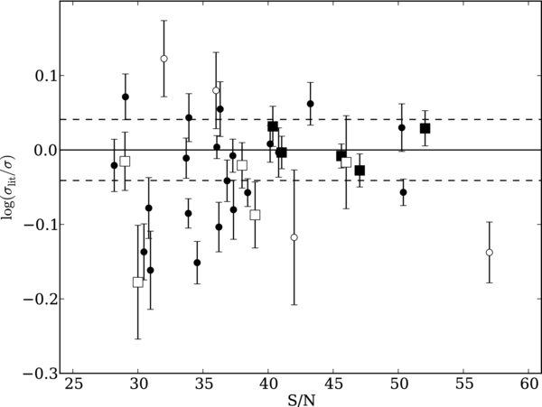
Figure 14. Comparison of our σ measurements to σlit, the measurements presented by Shen et al. (2008) (filled circles and squares) and Greene & Ho (2006a) (open circles and squares), as a function of the literature measurement S/N. Large squares mark measurements from objects common to all three studies (5 of 30). Here, our σ is the CaT equivalent measurement from the aperture spectrum at the Sloan fiber width (Column 4 of Table 2). Dashed lines represent a 10% difference.
Download figure:
Standard image High-resolution imageGreene & Ho (2006a) also investigates the fidelity of the MgIb and CaHK regions, though the MgIb region extends out to 5430 Å (and they caution that the Fe region redward of this is better to use) and the CaHK region is 3900–4060 Å. Since we correct our measurements for wavelength range bias and the biases are small (5%) we expect that our results are comparable to those of Greene & Ho (2006a) despite this difference. Greene & Ho (2006a) find that 〈(σMgIb–σCaT)/σCaT〉 = −0.23 ± 0.32 and 〈(σCaHK–σCaT)/σCaT〉 = −0.049 ± 0.29, i.e., both regions are consistent with CaT to within the (considerable) uncertainties. With our data set, we are able to reduce these uncertainties by a factor of 10 (and this is dominated by our systematic uncertainty). We find that σMgIb is higher than σCaT by 5% ± 3%, not lower; though the results agree to within error. Like Greene & Ho (2006a), we find that CaHK and CaT agree, with a 10 times stronger constraint on the uncertainty (≈3% compared to ≈30%).
Overall, we find good agreement between our measurements and those of similar studies in the literature, and we see that the high data quality of the Keck spectra compared to the SDSS fiber spectra allowed us to place much tighter constraints on the relationships between σCaHK, σMgIb, and σCaT than was previously possible.
9. SUMMARY
In this paper, we have presented deep long-slit spectroscopy for our spectroscopic sample of 96 AGNs and their host galaxies obtained at the W. M. Keck I 10 m Telescope. For the kinematic sample of 84 targets, the data are used to measure a homogeneous data set of rotation curves and stellar velocity dispersion profiles of unprecedented high quality. In future papers this set of measurements will be combined with black hole mass estimates and surface photometry to perform an accurate recalibration of the correlations between black hole mass and host galaxy properties in the local universe. In addition to providing all the measurements in tabular form, including SDSS-equivalent values of aperture stellar velocity dispersion, we use the data to investigate systematic effects in velocity dispersion measurements. Our findings can be summarized as follows.
- 1.Varying the spectral region used to measure stellar velocity dispersion introduces small systematic differences at the typical level of a few percent. Perhaps the only marginally significant bias is associated with using the MgIb region excluding the Fe features at central offsets, which can result in a bias up to 8% ±5%. We provide recipes to correct for these effects in Section 5.
- 2.Velocity dispersion measures based on the CaHK, MgIb regions can differ systematically by a few percent with respect to the reference region CaT. The MgIb bias is sensitive to AGN contribution in the spectrum. For apertures larger than ≈1'', σCaHK matches σCaT; for apertures larger than ≈2'', σMgIb is 5% ± 3% higher than σCaT, but the bias is a function of aperture width for apertures narrower than this.
- 3.It is possible to predict the probability of successfully measuring σCaHK from Sloan photometry and the EW of the Ca H&K features. Success rate is a strong function of color and EW. Targets with u − g > 0.7 or g − r > 0.5 are more than 50% likely to have a measurable σCaHK. This corresponds to a stellar fraction >80%. Targets with an EW<−4 Å are more than 50% likely to have a measurable σCaHK.
C.E.H. received funding for this research from the Summer Undergraduate Research Fellowship. C.E.H., V.N.B., and T.T. acknowledge support from the NSF through CAREER award NSF-0642621, and from the Packard Foundation through a Packard Fellowship to T.T. J.H.W. acknowledges support by Basic Science Research Program through the National Research Foundation of Korea funded by the Ministry of Education, Science and Technology (2010-0021558). Data presented in this paper were obtained at the W. M. Keck Observatory, which is operated as a scientific partnership among Caltech, the University of California, and NASA. The Observatory was made possible by the generous financial support of the W. M. Keck Foundation. The authors wish to recognize and acknowledge the very significant cultural role and reverence that the summit of Mauna Kea has always had within the indigenous Hawaiian community. We are most fortunate to have the opportunity to conduct observations from this mountain. This research has made use of the public archive of the Sloan Digital Sky Survey and the NASA/IPAC Extragalactic Database (NED) which is operated by the Jet Propulsion Laboratory, California Institute of Technology, under contract with the National Aeronautics and Space Administration.
Facility: Keck:I (LRIS) - KECK I Telescope
APPENDIX
A1. Testing the Stellar Kinematic Code
Motivated by the need to determine systematic uncertainties at the level of a few percent, we ran extensive Monte Carlo simulations to quantify how accurately our fitting program recovers the input value (σin) as a function of S/N and of σ. Consistent with previous work (e.g., Treu et al. 2001), we expect that for large values of S/N the code will return the input value, while as the S/N degrades significant biases might appear. Quantitatively, the amount of bias as a function of S/N and σ will depend on the exact instrumental configuration, chiefly the adopted wavelength range and resolution. To ensure a realistic test, the Monte Carlo realizations are obtained by adding random noise to the best-fit results of a subset of our galaxies, spanning a range in σ and each of the three wavelength regions.
The results of our tests are shown in Figure 15. For conciseness, we show only the test for the CaT region; the MgIb and CaHK regions give similar results. Gray bands of varying darkness show 1%, 5% (ideal target), and 10% accuracy. We use the median σ but include the results for the mean and most likely (maximum posterior) values for completeness; the median is generally most accurate, as can be seen in the figure. For the higher σin the code is well within our target accuracy, even at low S/N. As expected σ is least accurate for the lowest σin, as σin approaches the instrument resolution; however, we find that with S/N > 40 pixel−1 the code can recover σ to the desired accuracy even for the lowest σin. The difficulty of accurately recovering σ at low values of σ most likely causes the low-σ trends seen in panels (c) and (d) of Figure 11 (see Section 6.3).

Figure 15. Test of systematic bias in σ (for the CaT region 8480–8690 Å) as a function of S/N, for a range of input σ (σin) and three different ways of reporting σ—median, mean, and most likely value (ML; the maximum of the posterior). Gray bands mark 1%, 5%, and 10% accuracy. The measurements used in this work are the median σ, which we find to be the most accurate at low S/N. The target accuracy for our measurements and bias estimates is 5%. As expected, σ is more accurate for higher σin and the accuracy is less sensitive to S/N. Independent of σin, 5% accuracy is achieved by S/N ∼ 20 pixel−1.
Download figure:
Standard image High-resolution image